Node-Density Independent Localization Branislav Kusy, Akos Ledeczi
Miklos Maroti
Lambert Meertens
Vanderbilt University Nashville, TN 37212, USA
Department of Mathematics University of Szeged, Hungary
Kestrel Institute Palo Alto, CA 94304, USA
[email protected]
[email protected]
[email protected]
ABSTRACT This paper presents an enhanced version of a novel radio interferometric positioning technique for node localization in wireless sensor networks that provides both high accuracy and long range simultaneously. The ranging method utilizes two transmitters emitting radio signals at almost the same frequencies. The relative location is estimated by measuring the relative phase offset of the generated interference signal at two receivers. Here, we analyze how the selection of carrier frequencies affects the precision and maximum range. Furthermore, we describe how the interplay of RF multipath and ground reflections degrades the ranging accuracy. To address these problems, we introduce a technique that continuously refines the range estimates as it converges to the localization solution. Finally, we present the results of a field experiment where our prototype achieved 4 cm average localization accuracy for a quasi-random deployment of 16 COTS motes covering the area of two football fields. The maximum range measured was 170 m, four times the observed communication range. Consequently, node deployment density is no longer constrained by the localization technique, but rather by the communication range. Categories and Subject Descriptors: C.2.4[ComputerCommunications Networks]:Distributed Systems General Terms: Algorithms, Experimentation, Theory Keywords: Sensor Networks, Radio Interferometry, Ranging, Localization, Location-Awareness Acknowledgments: The DARPA/IXO NEST program has supported the research described in this paper.
1.
INTRODUCTION
We have recently proposed a novel approach to sensor node localization, the Radio Interferometric Positioning System (RIPS) [4]. RIPS creates a low-frequency interference signal by one pair of nodes transmitting simultaneously at close frequencies. The relative phase offset at a pair of receiver nodes is used to determine a distance measure between the transmitting and receiving nodes. Unlike tradiPermission to make digital or hard copies of all or part of this work for personal or classroom use is granted without fee provided that copies are not made or distributed for profit or commercial advantage and that copies bear this notice and the full citation on the first page. To copy otherwise, to republish, to post on servers or to redistribute to lists, requires prior specific permission and/or a fee. IPSN’06, April 19–21, 2006, Nashville, Tennessee, USA. Copyright 2006 ACM 1-59593-334-4/06/0004 ...$5.00.
tional ranging approaches, which determine the pairwise distance between two sensor nodes, RIPS measures dABCD , a distance aggregate called the “q-range” involving four nodes: two transmitters A, B and two receivers C, D. We reported a localization accuracy of 3 cm in a 16-node setup covering an area of 324 m2 . We estimated the maximum range of RIPS on Mica2 motes to be 160 m, but this was not experimentally verified.
1.1
New contributions
In this paper we show that, although not straightforward, the 160 m range is indeed attainable while keeping the ranging error down to a few centimeters. This result is a significant improvement over the existing ranging solutions in wireless sensor networks (WSNs), both in terms of the accuracy and the maximum range. A 160 m range is approximately four times larger than the actual communication range when deployed on the ground. Therefore, localization no longer needs to constrain the deployment of WSNs. Our analysis of interferometric ranging shows that it introduces significant ranging errors at large distances, which can be contributed to two major factors. The first problem is the ambiguity of the dABCD solution. Interferometric ranging computes the dABCD values from the phase offsets of the interference signal measured at two receivers C, D using the following equation: dABCD mod λ = ϕCD
λ , 2π
where ϕCD is the measured relative phase offset of the receivers, and λ is the wavelength of the carrier frequency of the received signal. In general, infinitely many dABCD values solve this equation. It was shown in [4] that measuring the phase offsets using different wavelengths (λ) can eliminate the incorrect solutions. However, the particular choice of wavelengths used in [4] yields ambiguous results for qranges larger than 57 m (or smaller than −57 m). Here we explore how to ensure that dABCD is unique. The second major error source is multipath radio propagation, which can distort the phase of the interference signal measured at the receivers. Multipath may become a significant error source with increasing node distances, even in the same relatively benign environment. The reason is that the ground-reflected radio signals are 180 degrees phase-shifted for small angles of incidence and travel almost the same distance as the direct line-of-sight (LOS) signal. Hence, the composite signal is attenuated and its amplitude becomes comparable to those of additional relatively weak multipath signals, causing noticeable phase deviations at the receivers.
We propose a novel ranging algorithm that executes q-range estimation and localization in an interleaved and iterative manner. That is, feedback from the current localization result is used to constrain the search space of q-range estimation, then the new estimates are used in the next localization phase, thereby iteratively refining the result. We show that this technique effectively corrects ranging errors and significantly improves the localization results. Today’s typical sensor network deployments are relatively dense, the nearest neighbor distance being at most 20 m. Consequently, the 160 m radius of the interferometric ranging can easily cover hundreds of sensor nodes introducing scalability problems for RIPS. Therefore, it is important to limit the amount of ranging data collected while ensuring that enough remains to solve the localization. First, we revisit the interesting problem of how many linearly independent interferometric ranging measurements exist for a set of n nodes and give a sharp upper bound improving the result given in [4]. Next, we present an algorithm that schedules the transmitters and receivers for the interferometric measurements. It limits the amount of acquired data and prevents uneven data sets that may otherwise result in the formation of well-localized clusters, but may not provide enough data to localize the whole network. We present an evaluation of the improved RIPS technique based on two experiments using XSM motes [2]. First, we deployed 50 motes in an 8000 m2 area with the neighbors 9 m apart. In this moderate multipath environment, we achieved a mean precision of 10 cm. In the second experiment, we deployed 16 motes in a rural area larger than two football fields. This setup demonstrated the maximum range to be 170 m, while the mean localization error was 4 cm. We organize the remainder of the paper as follows. Section 2 revisits the theoretical background of RIPS. Section 3 describes the problems we face when increasing the maximum range. Section 4 addresses the scalability issues. We evaluate our system in Section 5 and discuss related research in Section 6. Finally, we offer our conclusions and future directions in Section 7.
2.
INTERFEROMETRIC POSITIONING
Radio-based ranging techniques tend to estimate the range between two nodes from the known rate of radio signal attenuation over distance by measuring the radio signal strength (RSS) at the receiver. However, this technique is very sensitive to channel noise, reflections, interference from the environment among others. It was suggested in [4] to emit pure sine wave radio signals at two locations at slightly different frequencies. The composite radio signal has a low beat frequency and its envelope signal can be measured with low precision RF chips as the RSS Indicator (RSSI) signal (Figure 1). The phase offset of this signal depends on many factors, including the times when the transmissions were started. However, the relative phase offset between two receivers depends only on the distances between the two transmitters and two receivers and on the wavelength of the carrier signal. More formally, the following theorem was proven in [4]: Theorem 1. Assume that two nodes A and B transmit pure sine waves at two frequencies fA > fB , and two other nodes C and D measure the filtered RSSI signal. If fA −fB < 2 kHz, and dAC , dAD , dBC , dBD ≤ 1 km, then the relative
tsync
φD
φC
φCD
C D dAC
dBD dAD
dBC
A
B
Figure 1: Radio-interferometric ranging technique.
phase offset of RSSI signals measured at C and D is 2π
dAD − dBD + dBC − dAC c/f
(mod 2π),
where f = (fA + fB )/2. We call the ordered quadruple of distinct nodes A, B, C, D a quad and the linear combination of distances dAD −dBD + dBC − dAC for quad (A, B, C, D) the q-range dABCD . Note that the q-range is related to the range in the traditional sense, which is the distance between two nodes, but there is a significant difference between the two measures. If dmax is the maximum distance between any pair of the quad nodes, then the dABCD can be anywhere between −2dmax and 2dmax , depending on the positions of the four nodes. Next, denote by ϕX the absolute phase offset of the RSSI signal measured by node X at a synchronized time instant, the relative phase offset between X and Y by ϕXY = ϕX − ϕY , and the wavelength of the carrier frequency f of the radio signal by λ = c/f . Using this notation, Theorem 1 can be rewritten as dABCD mod λ = ϕCD
λ . 2π
ϕCD can be measured by the receivers C and D and λ is known. Note that a single ϕCD measurement does not yield a unique dABCD q-range because of the (mod λ) in the equation. However, we can measure ϕCD at different carrier frequencies, narrowing down the dABCD solution space until it contains a single q-range satisfying the maximum radio range constraint. Q-ranges can be used to determine 2D or 3D positions of the nodes, although the process is more complicated than determining positions from traditional ranges. An important difference between the interferometry and traditional ranging approaches is that we can measure at most n(n−3)/2 linearly independent q-ranges for a group of n
nodes, as shown in Section 4.1, as opposed to n(n−1)/2 linearly independent traditional pairwise ranges. Therefore, more nodes are required to determine the relative positions using interferometry. It was shown that at least 6 nodes are required to determine the 2D positions of all the nodes in the network and 8 nodes for 3D.
3.
MAXIMUM RANGE OF RIPS
As discussed before, RIPS is capable of measuring the relative phase offsets of relatively weak radio signals enabling ranging well beyond the communication range. Therefore, RIPS requires multi-hop communication and time synchronization. Furthermore, the original prototype introduced in [4] may incur significant ranging errors at large distances. We analyze the sources of these errors and suggest solutions to mitigate their effects in this section.
3.1
Ambiguity of q-ranges
Denote the relative phase offset of the receivers X and Y relative to the wavelength of the carrier frequency λ as λ , where ϕXY is the phase offset of X and Y . γXY = ϕXY 2π Theorem 1 can then be restated dABCD = γCD + nλ, where n ∈ Z, and both γCD and λ are known. Clearly, infinitely many dABCD values solve this equation (n is unknown). We can decrease the size of the dABCD solution space by measuring the phase offset γCD at m different carrier frequencies λi , giving γi , i = 1 . . . m. The resulting system of m equations has m + 1 unknowns, dABCD ∈ [−2dmax , 2dmax ], where dmax is the maximum distance between any pair of nodes, and n1 , . . . , nm ∈ Z: dABCD = γi + ni λi , i = 1 . . . m
(1)
Note that this system may still have multiple solutions. Before proceeding, we give a constraint on the ni for later use. The phase offsets are less than 2π, so |γi | < λi . From ni = (dABCD − γi )/λi and −2dmax ≤ dABCD ≤ 2dmax , we find |ni | < 2dmax /λi + 1. The problem is further complicated by measurement errors. The difference between the nominal and actual radio frequencies for a 100 ppm crystal causes an error in the wavelength of at most 0.0001 λ, which can be disregarded. But the error of the absolute phase measurement on the Mica2 hardware can be as high as 0.3 rad or 0.05 λ, according to our experiments, so the error of the relative phase offset γi can be as high as 0.1 λ. We denote the maximum phase offset error with εmax and rewrite equations (1) into the following (implicit) inequalities, i = 1 . . . m: dABCD ∈ [γi + ni λi − εmax , γi + ni λi + εmax ].
(2)
This system only has a solution if the intersection of these m intervals is non-empty. However, it is possible that the same system (with the same γi and λi values) has solutions for different assignments to the unknowns ni , in which case the system is ambiguous. Note, that the γi quantities cannot be controlled. Therefore, if we want to avoid the ambiguity problem, we need to choose values for the λi such that ambiguity is excluded. We now derive a necessary condition for ambiguity; by contraposition, its negation is a sufficient condition for avoiding ambiguity. So assume that also for some different vector of integers n0i , i = 1 . . . m, the intersection of the intervals [γi + n0i λi −
εmax , γi + n0i λi + εmax ] is non-empty, and let d0ABCD be a point in the resulting interval. Putting pi = ni − n0i , we have then, i = 1 . . . m: d0ABCD − dABCD ∈ [pi λi − 2εmax , pi λi + 2εmax ]. Since the intersection of these m intervals is non-empty, so is the intersection of any pair. This means that, for all pairs i, j in the range 1 . . . m: |pi λi − pj λj | ≤ 4εmax .
(3)
A further constraint on the pi values, which are integers, is found from the constraint given earlier on ni : |pi | = |ni − n0i | < 4dmax /λi + 2. The distinctness of the vectors ni and n0i , finally, requires at least one pi to be non-zero. If, conversely, we can find λi such that system (3) has no solution in integers pi —subject to the further constraints— then system (1) is guaranteed to be unambiguous for all possible outcomes for the γi . We put this in context by providing concrete characteristics of our radio driver used for the Chipcon CC1000 chip: the frequency range is 400–460 MHz, the minimum separation fsep between the possible frequencies is 0.527 MHz, and εmax is 0.075 m. Within these parameters, it is actually impossible to find a set of frequencies for which (3) is unsolvable. To start, there are solutions for very small pi . In particular, taking pi = 1 for all i, insolvability requires that εmax < 14 |λi − λj | for some pair i, j. But the range of wavelengths is 0.65– 0.75 m, requiring then that εmax < 0.025 m, way below the actually obtainable precision. In practice the situation is not that dire; for this to result in an actual ambiguity, all phasemeasurements errors have to “conspire”, with those for the smaller wavelengths being high (positive), and those for the larger wavelengths low (negative). For a set of, say, seven wavelengths, this is rather unlikely, although not impossible. Should an ambiguity of this type occur, and should the methods explained in subsection C below not lead to the correct disambiguation, then at least the error is not extremely large. Potentially much more pernicious are errors with large values of pi . To express them, we rewrite system (3) into |pi (λi − λj ) − (pj − pi )λj | ≤ 4εmax and then into |pi − (pj − pi )λj /(λi − λj )| ≤ 4εmax /(λi − λj ).
(4)
Putting d = pj − pi , we have then: pi ∈ [
4εmax dλj 4εmax dλj − , + ]. λi − λj λi − λj λi − λj λi − λj
It is easy to see that all large pi correspond to the integer λj λ λ multiples of λi −λ , which means errors of λii−λjj in dABCD j solution space. Note, that λi λj /(λi − λj ) corresponds to the wavelength c/fsep , where fsep = |fi − fj | is the frequency separation of fi , fj . We later use these two notions interchangeably. Fortunately, it is not hard to find relatively small “perfect” sets of frequencies, i.e., sets of frequencies for which such large errors are excluded. The carrier frequencies at which the phase offsets were measured in the previous work [4] were equally distributed in the 400–460 MHz range with fsep = 5.27 MHz, the wavelength of which is 57 m. Therefore, to increase the range, we currently use 0.527 MHz separation with wavelength of about 569 m, allowing q-ranges up to 275 m.
3.2
Multipath effects
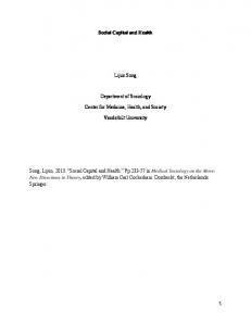
The results reported in [4] were obtained on a grassy area on campus near buildings and trees. As we experimented with extending the range of RIPS, the results quickly deteriorated. Once the cell size reached 10 m in the grid setup, the ranging error distribution got significantly worse. However, if we elevated the motes off the ground, the results improved markedly again. The nodes needed to be less than 10 m apart if they were on the ground, but could be more than 20 m apart if they were 4 feet high on tripods. Figure 2 shows representative phase offset measurements on 120 channels in the 400–460 MHz frequency range with the nodes on the ground (a) and 1.3 m elevated (b). Notice that the variance of the measured phase offsets is significantly smaller in the elevated scenario, while there are severe fluctuations in case of ground deployment. When we repeated the same experiment in a rural area far from buildings and trees, the results were very close to the ideal case irrespective of the deployment height. The last observation suggests that multipath propagation is at play here, but why does elevating the motes apparently fix the problem?
phase is −π, while for larger ones, it is 0. At a certain angle, called the Pseudo-Brewster Angle (PBA) [7], the phase is −π/2. The change from −π to 0 with increasing angle of incidence around the PBA is very steep. Thus, reflections at low angles have significant amplitude and opposite phase. As the distance difference between the line-of-sight (LOS) and the ground reflected signals is the smallest at small angles, the phase shift between them remains close to −π and hence, the composite signal is significantly attenuated. Figure 3 shows the simulation results of the effect of the ground reflected signal on the LOS wave over average ground surface. We used a two-node setup, where the distance between the nodes was fixed at 30 meters, while we elevated the nodes off the ground up to 5 meters—sweeping the angle of incidence between 0 and 20◦ . The figure shows the amplitude coefficient and the received composite signal, for which the path loss was simulated (both for the direct and reflected signals) using λ2 /(4πd)2 decay. We experimentally validated the results for a smaller range of angles in a rural area where no multipath effects were present other than ground reflections and obtained data similar to the predicted values.
18 -6
16
5
1
8 measured phase offset
4 2 390
expected phase offset 400
410
420
430
440
450
460
carrier frequency (MHz)
(a) 18 16
4
0.8 Composite Signal
3
0.6
2
0.4
1
Amplitude Coefficient
14
0.2
Reflected Amplitude Coefficient (A)
10
6
phase offset (rad)
x 10
12
Composite Signal Amplitude (S)
phase offset (rad)
14
12
0
10 8
0
5
10 15 Angle of Incidence (Degrees)
0 20
6
measured phase offset 4 2 390
expected phase offset 400
410
420
430
440
450
460
carrier frequency (MHz)
(b) Figure 2: Phase offset measurements on 120 channels with vertical monopole antennas directly on the ground (a) and 1.3 m elevated (b). Up till now, we have considered the radio nodes as if they were operating in free space. However, the ground around and under the antenna and other nearby objects such as trees or buildings can have significant impact on the shape and strength of the radiated pattern. These interactions can be explored in two distinctive regions surrounding the antenna. The reactive near field is within one quarter of the wavelength, therefore we do not consider it in this paper. In the radiative far field, ground reflections—especially for vertically polarized antennas—and additional paths through reflective objects profoundly influence the received signal. When the radio wave strikes a surface, it is reflected with an angle that is equal to the angle of incidence. For surfaces with infinite conductivity, the reflected wave has the same amplitude and the same phase—or opposite, depending upon polarization—as that of the incident signal. For real surfaces, the reflected amplitude tends to be smaller and the phase relationship is more intricate. At small angles, the
Figure 3: The reflection coefficient and the amplitude of the composite signal for vertically polarized waves. The composite signal is shaped by the interplay of the decreasing ground-reflection coefficient, and the phase offset and attenuation change due to the increasing distance the reflected signal travels. We observed that the amplitude of the composite signal grows tenfold when we elevate the nodes from ground level to 1 m (at 30 m distance). This significant attenuation is not a problem in and of itself, as long as we can still measure the phase of the signal accurately. It definitely decreases the effective range of the method, but it does not by itself impact the accuracy noticeably. However, in a moderate multipath environment, such as the campus area we used, reflections from buildings and other surfaces distort the results. As these reflections travel longer distances, they are markedly attenuated. As long as the direct LOS signal is strong, the additional phase shift these components cause is small. However, when the ground reflection significantly attenuates the LOS signal, the phase shift caused by additional multipath components is large enough to distort the results considerably, as shown in Figure 2. We found that the measured strength of the received signals (not shown in the figure) was 8 dB stronger with elevated nodes. Since the overall topology, the node-to-node distances and the environment
were identical in the two measurements, we have experimentally verified that the differences are indeed caused by the angle—thus elevation—dependent ground reflection.
3.3
Coping with the q-range error
Intuitively, solving the ranging problem can be thought of as fitting a straight line to the measured data. As shown in Figure 2, the ideal phase offset is linear as a function of the frequency if we allow for wraparound at 2π. If we have data distorted by multipath and other errors, we can still fit a line relatively accurately, provided we have enough good data points. Therefore, a trivial enhancement is to make measurements at as many frequency channels as possible. However, this also increases the required time of the actual ranging, and a balance must be struck. We now show how to further improve the q-range estimation and the overall localization results, even in the face of q-range ambiguity and moderate multipath effects. Let us first revisit how the baseline q-range estimation works.
1. Initialize the value of R, the search radius, and set all q-range estimates to 0. 2. Calculate the q-range estimates by finding the minimum of the sum of the phase-offset discrepancy functions, searching within radius R from the current qrange estimates. 3. Calculate optimal node locations. 4. If R is small enough, stop. Otherwise, decrease R and go to step 2.
0.35 mean square error
vations were made: 1. If 30–40% of the q-ranges have less than 30 cm error, the localization algorithm converges and finds approximate locations with errors smaller than a few meters. 2. Even in multipath environments the phase-offset discrepancy function has a sharp local minimum at the real q-range in most of the cases. See Figure 4. These two observations led to the idea of the iterative phase-offset discrepancy correction algorithm:
1 2
0.3
3
0.25 0.2 0.15 2
0.1
3 1
0.05
13.3
11.3
9.24
7.22
5.19
3.17
-0.9
1.16
-4.9
-2.9
-6.9
-11
-8.9
-13
-15
0 range (m)
Figure 4: Phase-offset discrepancy function in a severe multipath environment. The numbers show the search intervals of consecutive error correction iterations and the corresponding minima. The spot labeled 3 is the real solution. To get the q-range dABCD we have to solve the inequalities (2). Given a possible q-range r, for each i we can find the value of n “i that” brings γi + ni λi the closest to r, namely i ni = round r−γ . Then we define the phase-offset disλi crepancy function to be the average value of the squares of γi +ni λi −r values as a function of r. Ideally, the global minimum of the discrepancy function is 0, attained at the true q-range. However, measurement errors, multipath effects and the ambiguity due to the limited number of channels and the minimum channel separation, distort the results. Frequently, the global minimum is not at the true solution. Figure 4 shows an example of the phase-offset discrepancy function in a severe multipath environment indoors. The true q-range is at the local minimum labeled 3. Given a sufficient number of q-range measurements, it is possible to estimate the node locations (up to Euclidean isometric transformations) by finding the locations that minimize the q-range discrepancy, defined as the average value of the squares of the differences between each measured qrange and the corresponding q-range “on the map”, i.e., the dABCD value computed from the node locations. After analyzing several experiments, the following obser-
In other words, the current localization solution is used to constrain the search space of the ranging algorithm, so that it can progressively eliminate large errors. Due to this feedback method, the q-range estimates get more and more accurate at each iteration. It is easy to see that if the current value of R is always larger than the maximum q-range error in our current localization, bounding the search will not exclude the correct q-range. In our current prototype, we use fixed decreasing R values, such as R1 = 50 m, R2 = 5 m, R3 = 0.5 m. The difference between the measured q-range and the corresponding q-range on the map is known and has a strong correlation with the localization error. This distance error could be used to drive the actual value of R and make this iterative method more adaptive. We leave this idea as a topic for future research.
4.
SCALABILITY OF RANGING IN TIME
We revisit the theoretical bound on the maximum number of linearly independent q-range measurements for a set of n nodes, improving the result given in [4].
4.1
Independent q-range measurements
We assume that the network has at least three nodes, and that the nodes forming the network are numbered 0 through n−1. Let N = {0 . . n−1} denote the set of nodes. In the notation dAB , we always assume that A and B are nodes in N . By convention, dBA means the same as dAB . Clearly, there is no need to determine quantities dAA , so without loss we require in the notation dAB that A 6= B. Then in the network there are in all n(n−1)/2 such quantities dAB . These distances are not independent in the sense of being mutually unconstrained. To start with, there is the triangle inequality: dAC ≤ dAB +dBC . Assuming that the nodes live in Euclidean 2D space, there is the further constraint that the Cayley-Menger determinant on any quad (A, B, C, D) vanishes. Here we are concerned with a more technical notion of independence: linear independence of a collection of vectors in a vector space. Recall that, given a vector space V and a set of vectors {vi } of V , the subspace spanned by that set consists of the
P collection of vectors that can be written as i λi vi for some assignment of scalar valuesP λi . The set of vectors is called linearly independent when i λi vi = 0 ≡ ∀i λi = 0. A basis of V is then a linearly independent set of vectors of V that spans V . Now take an n(n−1)/2 dimensional vector space over the field of the real numbers, and label the vectors of some basis with dAB , for A and B distinct nodes from N — also here label dAB is identified with label dBA . Define, for quad (A, B, C, D), dABCD = dAD − dBD + dBC − dAC . Thus defined, dABCD is a vector in our vector space. We call it a measurement, because it corresponds to a possible measurement that could be carried out by the radiointerferometric technique, the outcome being (modulo experimental error) the value of the right-hand side under some valuation of the basis vectors dAB . Clearly, dABCD + dBACD = 0 and dABCD − dCDAB = 0, so these vectors are not all mutually independent. To rule out these pairwise dependencies, we require that in any index ABCD we have: A < B, A < C < D, B 6= C, B 6= D , in which the last two inequalities, required by the distinctness of the four nodes, are given for the sake of completeness. We call an index satisfying these inequalities normalized. If some of the other inequalities are violated, the corresponding measurement can be found from one with a normalized index by using the pairwise dependencies given above. Since there are three orderings of A, B, C and D compatible with the index inequalities, A