{kegen.yu, mark.hedley, ian.sharp, jay.guo}@csiro.au. Abstractâ Locating the sensor nodes in an ad hoc wireless sensor network (WSN) is a very challenging ...
Node Positioning in Ad Hoc Wireless Sensor Networks Kegen Yu, Mark Hedley, Ian Sharp and Y. Jay Guo Wireless Technologies Laboratory CSIRO ICT Centre Marsfield NSW 2122, Australia {kegen.yu, mark.hedley, ian.sharp, jay.guo}@csiro.au
Abstract— Locating the sensor nodes in an ad hoc wireless sensor network (WSN) is a very challenging task. In general, the network nodes are not synchronised and the internal delays within the sensor nodes may be unknown. As a result, the positioning problem can not be solved by simply using the triangulation method and certain prior information must be provided. In this paper, we consider a scenario where there are a number of nodes whose positions are known, and it is required to locate the other mobile or static sensor nodes within the radio range of each other by measuring the time of arrival (TOA) in the whole system. Two algorithms are employed, the direct method and the linear least squares (LS) estimator. The performance of the two algorithms is investigated. In particular an analytical formula is derived to estimate the performance of the LS estimator. Simulation results agree well with theoretical predictions.
VI shows some simulation results of the two location estimation methods. Finally, the conclusions are given in section VII. II. M EASUREMENT E QUATIONS C ONSTRAINTS
• • •
The sensor nodes are not synchronised and there are unknown clock offsets among them; The internal delay within each sensor node is treated as another unknown parameter; The TOA measurement error due to factors such as multipath is modelled as a non zero mean random variable.
Two non-iterative methods, the direct method and the linear least squares (LS) estimator are used to find the locations of the sensor nodes. Theoretical analysis and simulations are employed to evaluate the performance of the algorithms. The paper is organised as follows. In section II, the general frame work for the study is presented and the minimum information required to find the node locations is discussed. The theory of the direct method is presented in section III, and that for the LS estimator is presented in section IV. In section V, the analytical performance of the LS estimator is derived. Section
rx c φci +∆tx i +τi,j +∆j −φj = Ti,j ,
where τi,j = τj,i =
i, j = 1, . . . , N, i �= j, (1)
� (xi − xj )2 + (yi − yj )2 /c
(2)
is the direct time-of-flight (TOF) of the radio signal between nodes i and j, φck , k = i, j, is the clock phase, ∆tx i is the system internal delay between the clock and the transmit antenna, ∆rx i is the delay between the clock and the receive antenna, and Ti,j is the TOA of the signal received at node j and transmitted at tx rx node i. Let φk = φck + ∆tx k and ∆k = ∆k + ∆k . Then, (1) becomes τi,j + φi + ∆j − φj = Ti,j .
(3)
As a result, each node has only two time parameters involved: the internal delay ∆k and the clock phase φk . Under the assumption of no frequency error, there are four parameters for each node: two time parameters and two coordinate parameters. Therefore, there are 4N parameters in a network of N nodes. When one of the clock phases is taken as the reference, there are 4N − 1 parameters. A question may arise: what is the minimum information (either time or position parameters) required a priori to determine the unknown position coordinates? Note that some of the equations in (3) may be dependent on the others. When the number of the independent measurement equations is greater than that of the unknown parameters, the system is over-determined. In the case of the number of the unknown parameters equal to the number of the independent equations, the system is exactly-defined. In both cases, a solution can be found for each unknown parameter. However, in the event that the number of the unknowns is greater than the number of the independent equations, the system is under-determined and information of some parameters should be given to solve the equations to produce a solution to each of the unknowns. When is the system given by (1) over-, exactly-, or under-defined? It would be interesting to answer the question and the key point is to find out the number of the independent equations in (1). Table I shows the number (Nind ) of independent equations when there are N nodes in the network. Theorem 1: In the case of N (N > 1) nodes, the number of independent TOA measurement equations in (3) is given by
641 0-7803-9701-0/06/$20.00 ©2006 IEEE
M INIMUM
Consider a network of N nodes and each pair of nodes has a communication link. Let (xi , yi ) be the coordinates of the i-th node. When each node transmits a packet which is received by the other N − 1 nodes, there are N (N − 1) TOA measurements, corresponding to N (N − 1) measurement equations:
I. I NTRODUCTION The location information of nodes in wireless sensor networks (WSN) is very important for many applications, such as asset tracking, patient monitoring and personnel management in rescue operations. Although GPS can offer high accuracy in outdoor environments, it often doesn’t work indoors and can be uneconomical to be used in large scale networks. A simple method for indoor positioning is based on the measurement of received signal strength (RSS) [1], but this method normally results in very poor accuracy due to the unpredictable variance of radio wave attenuation in multipath environments. In a practical ad hoc wireless sensor network, the unknown parameters are not only the co-ordinates of the nodes but also the clock offsets and internal delays within the nodes. To find the co-ordinates of all the sensor nodes in the network, some prior information must be provided. In this paper, we consider the following scenario: there are a number of sensor nodes in the network whose positions are known. The positions of the other sensor nodes, being static or mobile, are estimated by measuring the time of arrival (TOA) in the whole system. The assumptions made for the analysis include the following:
AND
N Np Neq Nind
2 7 2 2
3 11 6 5
4 15 12 9
5 19 20 14
6 23 30 20
7 27 42 27
8 31 56 35
where
TABLE I N UMBER OF INDEPENDENT EQUATIONS VERSUS NUMBER OF NODES . Np : NUMBER OF PARAMETERS . Neq : NUMBER OF TOA EQUATIONS .
Nind =
1 N (N + 1) − 1 2
(4)
The proof of the above results is omitted to save space. Note that the results in table I are produced by treating the TOF τi,j as a variable. Although the system in (1) is over-defined for N > 7 without any a priori information of the parameters, the position coordinates might not be determined. This is due to the fact that any constant offset of all coordinates would keep the TOF or the distance between a pair of nodes constant. To have the position parameters determined, a (local) coordinate system needs to be developed. One common way to establish such a system is as follows. Choose three nodes and first map the spatial origin to one node such that (x1 , y1 ) = (0, 0). Another node is then assigned to (x2 , y2 ) = (d2,1 , 0) where d2,1 is the distance between the two nodes. Finally the y-coordinate of a third node is positive. In this case, the number of parameters in Table I should be reduced by three. III. D IRECT M ETHOD Let us first consider the case of four nodes in the network. Three nodes are fixed and their locations are known a priori. The other node is the mobile, static or moving, which is to be located. So it satisfies the minimum requirement given in section II, which requires six known parameters to determine the others. Throughout the paper, we ignore the TOA error in developing the location algorithms for notational simplicity, while the error-free TOA parameter is replaced by the imperfect TOA measurement in the final solution to the position estimate. Assume that the position coordinates of the three fixed nodes are defined as (xi , yi ), i = 2, 3, 4 and the unknown mobile position is denoted by (x1 , y1 ). Then, the TOA equations are: � (xi − xj )2 + (yi − yj )2 /c + φi + ∆j − φj = Ti,j , i, j = 1, 2, 3, 4, i �= j,
(5)
where ηi,j = Ti,j
(6)
η3,2 η2,3 η4,2 r= η4,3 . η2,4 η3,4
where W is the weighting matrix which emphases the contributions of the measurements that are more reliable. For instance, measurements with a higher received signal-to-noise ratio (or simply a higher received signal power) should be weighted more. In the absence of a priori confidences, the weighting matrix may be simply chosen to be an identity matrix. Let us move on to estimate the mobile position. When the mobile is either the transmitter or the receiver, (5) becomes � (x1 − xj )2 + (y1 − yj )2 /c + φ1 + ∆j − φj = T1,j , (9) � (x1 − xj )2 + (y1 − yj )2 /c + φj + ∆1 − φ1 = Tj,1 (10) There are three equations in (9) with three unknowns, x1 , y1 , and φ1 so that a unique solution should be available for each unknown. However, to make use of the extra measurements in (10), we may average the measurements by adding (9) to (10), producing � (x1 − xj )2 + (y1 − yj )2 = bj − ∆1a , j = 2, 3, 4, (11) where bj = c(T1,j + Tj,1 − ∆j )/2 is known while ∆1a = c∆1 /2 is unknown. Squaring both sides of (11) yields (x1 − xj )2 + (y1 − yj )2 = ∆21a + 2bj ∆1a + b2j
(12)
Subtracting (12) for j = 3, 4 by (12) for j = 2 gives x2,j x1 + y2,j y1 = b2,j ∆1a + g2,j , j = 3, 4,
(13)
where xi,j = xi − xj ,
yi,j = yi − yj , gi,j = 0.5(x2i + yi2 − (x2j + yj2 ) + b2j − b2i )
Solving (13) for x1 and y1 in terms of ∆1a , we have x1 = h1 ∆1a + f1 ,
y1 = h2 ∆1a + f2 ,
(14)
where hi = ξi,1 b2,3 + ξi,2 b2,4 , fi = ξi,1 g2,3 + ξi,2 g2,4 , i = 1, 2. Here ξi,j are the elements of the matrix �−1
x2,3 y2,3 . x2,4 y2,4 Substituting (14) into (12) for j = 2 produces (15)
where E = h21 + h22 − 1,
Equation (6) can be written in compact form as
642
∆2 φ3 θ= ∆3 , φ4 ∆4
E∆21a + 2F ∆1a + G = 0
� − (xi − xj )2 + (yi − yj )2 /c.
Aθ = r
0 0 0 1 0 0 0 1 0 , 1 1 0 0 −1 1 0 −1 1
The standard LS estimator can be employed to the slightly overdetermined system and the solution is � −1 T θˆ = AT WA A Wr (8)
bi,j = bi − bj ,
where it is assumed that all node clocks run at the same rate and the effect of clock frequency offset will be investigated by simulation. As the positions of the fixed nodes are known, we may first determine the unknown time parameters of the fixed nodes. Without loss of generality, we let the clock phase of the node that initiates the communication be zero, say φ2 = 0. Then from (5), we have φi + ∆j − φj = ηi,j , i, j = 2, 3, 4, i �= j,
1 1 0 −1 1 0 A= 0 −1 0 0 0 1
(7)
F = h1 (f1 − x2 ) + h2 (f2 − y2 ) + b2
G = (f1 − x2 )2 + (f2 − y2 )2 − b22
2006 IEEE International Conference on Industrial Informatics
The solution to the quadratic equation (15) is given by � 2 F F G ∆1a = − ± − E E E
where (16)
Substituting (16) into (14), we obtain the estimate of the mobile position. Clearly, there exist two solutions and only one of them is the desirable. We remove the one either with no physical meaning or which is beyond the monitored area. In the event that both solutions are reasonable, an ambiguity occurs. However, the ambiguity may be cleared by choosing the solution that minimizes �2 4 � � (x1 − xj )2 + (y1 − yj )2 − (bj − ∆1a ) . (17) j=2
∆ = [∆q+1 , ∆q+2 , . . . , ∆N ]T ∈ R(N −q)×1 , (24) r = [rq+1,q+2 , . . . , rq+1,N , rq+2,q+3 , . . . , rq+2,N , . . . , rN −1,N ]T ∈ R((N −q)(N −q−1)/2)×1 ,
and A is a matrix of dimensions of ((N − q)(N − q − 1)/2) × (N − q). The weighted LS solution to (23) is � ˆ = AT WA −1 AT Wr ∆ (26) When considering the measurements from each pair of a mobile and a fixed node, (20) becomes � 2 (xi − xj )2 + (yi − yj )2 /c + ∆i = Ti,j + Tj,i − ∆j , i = 1, 2, . . . , q, j = q + 1, q + 2, . . . , N, (27)
IV. L INEAR LS E STIMATOR In the preceding section we derived the exact solutions to the position parameters in the case of four nodes. When there is a communication link among more than four nodes, it would be desirable to make use of the extra measurements to improve the location accuracy. In this section, we employ the non-iterative linear LS estimator for position location. Without loss of generality, suppose that the positions of q nodes, (xi , yi ), i = 1, 2, . . . , q, are to be estimated, while the positions of N − q nodes, (xi , yi ), i = q + 1, q + 2, . . . , N , are known a priori. For simplicity, the q nodes to be located are called mobile nodes while the other N −q nodes are termed fixed nodes. Also assume that each mobile node has a communication link with at least four fixed nodes1 . Rewrite the TOA equations as � (xi − xj )2 + (yi − yj )2 /c + φi + ∆j − φj = Ti,j , i = 1, 2, . . . , N − 1, j = i + 1, . . . , N, � (xi − xj )2 + (yi − yj )2 /c + φj + ∆i − φi = Tj,i .
(25)
Moving ∆i to the other side of (27) and then squaring both sides, we have (i)
Ri2 + Rj2 − 2xj xi − 2yj yi = (bj − 0.5c∆i )2 where (i)
bj = 0.5c (Ti,j + Tj,i − ∆j ) ,
Rk =
(28)
� x2k + yk2 .
Subtracting (28) for j = q + 2, q + 3, . . . , N by (28) for j = q + 1, we obtain (i)
(i)
2xq+1,j xi + 2yq+1,j yi − cbq+1,j ∆i = βq+1,j , i = 1, 2, . . . , q, j = q + 2, q + 3, . . . , N, (29) where
(18)
xk,j = xk − xj , yk,j = yk − yj ,
(19)
bk,j = bk − bj , βk,j = Rk2 − Rj2 + (bj )2 − (bk )2 . (30)
(i)
(i)
(i)
(i)
(i)
(i)
Intuitively, the computation can be reduced by adding (18) and (19) to produce � 2 (xi − xj )2 + (yi − yj )2 /c + ∆i + ∆j = Ti,j + Tj,i , (20)
The unknown coordinates can be determined either jointly or separately and the results should be the same. When solving separately, write (29) in compact form
where the clock phases are completely removed. Then, the unknown coordinates can be determined by solving the N (N − 1)/2 equations in (20). Consider a two-step location procedure similar to what we employed in section III. First, use the position information of the fixed nodes to estimate their internal delays. The estimates are then employed to locate the mobile nodes. When only considering the measurements among the fixed nodes, (20) can be written as
where
∆i + ∆j = ri,j , i = q + 1, q + 2, . . . , N − 1, j = i + 1, . . . , N, (21) where ri,j = Ti,j + Tj,i − 2τi,j .
(22)
Write (21) in compact form: A∆ = r,
(23)
1 When a mobile is located, its position and time information may be employed to locate other nodes. In this case, it is not necessary for a mobile to have a link with four or more fixed nodes.
Ai pi = βi , 2xq+1,q+2 .. Ai = . 2xq+1,N
i = 1, 2, . . . , q,
2yq+1,q+2 .. . 2yq+1,N
(i) −cbq+1,q+2 ∈ R(N −q)×3 , ... (i) −cbq+1,N
pi = [xi , yi , ∆i ]T ∈ R3×1 , (i)
(i)
(i)
βi = [βq+1,q+2 , βq+1,q+3 , . . . , βq+1,N ]T ∈ R((N −q))×1 . (31) Applying the weighted LS estimator, we obtain � −1 T ˆ i = ATi Wi Ai p Ai Wi βi ,
(32)
where Wi is the weighting matrix. Once the coordinates of a node are estimated, they may be employed to determine the coordinates of the other mobile nodes, especially when a mobile does not have a link with enough fixed nodes. Compared to the iterative algorithms such as the Taylor series method [2, 3] and the optimization based approach [4], the direct method and the linear LS estimator involve less computation [5] and do not have the convergence issue.
2006 IEEE International Conference on Industrial Informatics
643
V. P ERFORMANCE
OF
L INEAR LS ESTIMATOR
In this section, we are interested in deriving the analytical performance of the LS estimator described in section IV, in terms of mean (bias), variance, and cumulative distribution function (cdf) of the coordinate estimation error. Suppose that the error of the TOA measurement, Tˆi,j − Ti,j , is a random variable of mean µi,j (due to the multipath effect) and variance 2 σi,j . Also assume that each TOA measurement is independent from the others. Then, Tˆi,j − Ti,j + Tˆj,i − Tj,i 2 2 is a random variable of mean µi,j + µj,i and variance σi,j + σj,i . To work out the mean and variance of the location error, let us first determine the mean and variance of the delay estimation error from (26). In the small error region, expanding the delay error in a Taylor series and retaining the first two terms produce
ˆ −∆= �∆ = ∆
N1 � ∂∆ i=1
∂ri
(ˆ ri − ri )
(33)
where ri is the i-th element of r (defined in (25)). N1 = (N − q)(N −q −1)/2 and can be found to be the i-th column � ∂∆/∂r i−1 AT W in (26). As a result, we vector of matrix AT WA obtain the mean and variance of the delay estimation error as: � N1
� ∂∆ E[�∆j ] ≈ E[ˆ ri − ri ], ∂ri j−1,1 i=1 j = q + 1, q + 2, . . . , N,
Var[�∆j ] ≈
�2 N1
� ∂∆ i=1
∂ri
Var[ˆ ri − ri ].
(34) (35)
j−1,1
Before proceeding further, let us simplify the problem by ˆi = assuming ∆i is known such that pi = [xi , yi ]T , and p [ˆ xi , yˆi ]T . Then, (32) becomes −1 T � ˆ i = GTi Wi Gi p Gi Wi αi , (36) where Gi is part of Ai and equal to the remainder when the third column of Ai is removed, and αi has the same expression (i) as βi given by (30) and (31), except that bj is replaced by (i)
bj = 0.5c (Ti,j + Tj,i − ∆j − ∆i ) .
(37)
ˆ i (in (36)), Then, in the same way, we can expand the estimate, p in a Taylor series as: ˆ i − pi ≈ p where
N � ∂pi ˆ(i) (i) (b − bj ), (i) j ∂b j=q+1 j
(38)
� � ˆb(i) − b(i) = c (Tˆi,j − Ti,j ) + (Tˆj,i − Tj,i ) − (∆ ˆ j − ∆j ) j j 2 (39) is a random variable of mean c� (i) (i) µi,j + µj,i − E[�∆j ] , (40) E[ˆbj − bj ] = 2 and variance c2 � 2 (i) (i) 2 Var[ˆbj − bj ] = + Var[�∆j ] . (41) σ + σj,i 4 i,j The partial derivatives can be found to be −1 T � ∂αi ∂pi = GTi Wi Gi Gi Wi (i) , j = q +1, q +2, . . . , N, (i) ∂bj ∂bj (42)
644
where � � ∂αi
(i)
(i)
∂bq+1 k � � ∂αi (i) ∂bj
k
= −2bq+1 , 1 ≤ k ≤ N − q � =
(i)
2bj 0
(43)
k = j − q − 1, , q + 1 < j ≤ N. (44) elsewhere,
Therefore, the mean of the coordinate estimation error is � � N � � � ∂pi (i) (i) E[ˆ xi − xi ] ≈ E ˆbj − bj , (i) j=q+1 ∂bj 1,1 (45) � � N � � � ∂p i (i) (i) E[ˆ ˆ E bj − bj , yi − yi ] ≈ (i) j=q+1 ∂bj 2,1 and the variance is � �2 N � � � ∂pi ˆb(i) − b(i) , Var[ˆ x − x ] ≈ Var i i j j (i) j=q+1 ∂bj 1,1 � �2 N � � � ∂p i ˆb(i) − b(i) . Var[ˆ yi − yi ] ≈ Var j j (i) j=q+1 ∂bj 2,1
(46)
Due to the fact that ∆i is treated as a known error-free parameter, the derived performance may be approximated as a lower bound. Another location performance measure is the percentage of the repeated location measurements which are within a circle of a specific radius and whose center is the actual location [6]. This measure is similar to the circular error probability proposed by Torrieri [3]. Equivalently, we consider the cumulative distribution of the location error. Suppose that both the x-coordinate error �x and the y-coordinate error �y are Gaussian distributed 2 with mean µ�x and µ�y , and variance σ�2x and σ�2y , respectively. Then, � (47) � = �2x + �2y , has a Rayleigh distribution whose cumulative distribution function is given by
� �2 F (�) = 1 − exp − 2 , (48) 2σ for the case of µ�x = µ�x = 0 and σ�2x = σ�2y = σ 2 . When σ�2x �= σ�2y , let σ 2 = 0.5(σ�2x + σ�2y ). In the event of either µ�x �= 0 or µ�y �= 0 , � has a Rice distribution [7] whose cdf is � µ2�x + µ2�y � , , (49) F (�) = 1 − Q1 σ σ where Q1 (a, b) is the Marcum Q-function which is defined as
2 � ∞ ∞ a + b2 � � a �k � (ab/2)k+2� . Q1 (a, b) = exp − 2 b !Γ(k + + 1) k=0
�=0
As a summary, first compute the mean and the variance of the two coordinate errors by (45) and (46), respectively. If the two means are zero, use (48) to compute the cumulative distribution. Otherwise, employ (49) to calculate the distribution. 2 The assumption becomes true when the TOA measurement error is Gaussian. When the TOA error is not Gaussian, the coordinate error could be approximated Gaussian especially in the event of relatively large N .
2006 IEEE International Conference on Industrial Informatics
5 STD of Position Estimate (m)
Cumulative Distribution (100%)
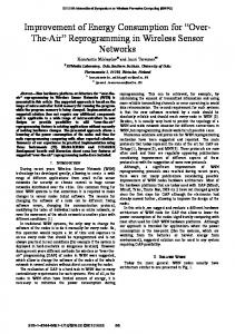
1 0.8 0.6 0.4 FO=0 FO=0.01ppm FO=0.02 FO=0.05
0.2 0 0 Fig. 1.
1
2 3 Localization Error (m)
VI. S IMULATION R ESULTS Let us first examine the performance of the algorithm described in section III. The simulation setup is as follows. The dimensions of the monitored area are 30m × 30m; and the positions of the fixed nodes are chosen to be (0, 4), (30, 4), and (15, 30); • The radio range of all nodes is set at 30 meters; • The square of 30m×30m is divided into 3,600 equal squares of side length 0.5 meters; The mobile position changes from one small square to the other, in the order of from left to right and from top to bottom. • The clock offsets are randomly chosen between -0.5 and 0.5 seconds; The system delay is treated as a Gaussian random variable of mean 600 nanoseconds (ns) and standard deviation (STD) 10 ns. • The TOA measurements are in error due to: the multipath effect and the error is modelled as a Rayleigh distributed random variable of mean 6.27 ns and STD 3.28 ns; and the receiver noise and the error is assumed to be Gaussian of mean zero and STD two nanosecond. Fig. 1 shows the error cumulative distribution of the location algorithm. Several clock frequency offsets are examined. Clearly, frequency offset degrades positioning performance substantially even for frequency offset equal to 20 parts per billion (ppb). Therefore, frequency offset estimation and compensation is required to achieve desirable performance in the event that only practical and affordable crystal oscillators are available. In the system, we employ a simple frequency synchronization scheme which we do not discuss in this paper. It can be seen that the percentages of the estimation accuracy of 2 and 3 meters are about 82, and 93, respectively, in the absence of frequency offset error. Note that the weighting matrix is simply taken as the identity matrix throughout the simulation. Choosing efficient weighting matrices will be our future research. Fig. 2 shows the simulated and analytical results (STD) of the LS estimator when there are four, five, or six fixed nodes which are placed according to: •
• •
Four fixed nodes: (0, 4), (30, 4), (15, 30), and (15, 13); Five fixed nodes: (0, 4), (30, 4), (15, 30), (10, 13), and (20, 13);
3 2 1 0 0
4
Cumulative distribution of position estimation error.
4
simulated(5 nodes) simulated(6 nodes) simulated(7 nodes) approx(5 nodes) approx(6 nodes) approx(7 nodes)
2 4 6 8 STD of TOA Error Due to Noise (ns)
10
Fig. 2. Standard deviation of the location error when using the linear LS estimator.
Six fixed nodes: (0, 4), (30, 4), (15, 30), (10, 10), (20, 10), and (15, 19). The deployment of the fixed nodes can have a significant impact on the location performance. In [8], three of four fixed nodes are uniformly spaced around a circle and the fourth is placed at the center of the circle. In [9], the fixed nodes (beacons) are uniformly placed on a grid of points in the monitored area. We chose the layout based on the numerical results under the radio range consideration. Clearly, more fixed nodes result in better performance. Also we can see that the analytical results play a lower bound on the simulated results. The approximated bound becomes tighter as the number of fixed nodes increases. The mean of the estimation error is not presented since both the analytical and simulated means are close to zero. Fig. 3 shows the simulated and analytical cumulative distributions of the location error when using the LS estimator, which correspond to the results shown in Fig. 2 when the STD of the TOA error due to noise is two nanoseconds. The analytical cdf is computed using (48). Clearly, there is a good match between the simulated and the analytical results, especially when there are more than five nodes in the network. Note that the analytical cdf does not lower-bound the performance of the estimator. The reason is that we assumed the coordinate estimation error is Gaussian; however, it could not be Gaussian due to the Rayleigh distributed TOA error resulted from the multipath effect. •
VII. C ONCLUSIONS In the paper, we developed two algorithms for node location in ad hoc wireless sensor networks in an indoor environment. The performance of the algorithms were evaluated under realistic considerations. The network considered is not synchronized such that a clock offset exists between each pair of nodes. The system delay is treated as an unknown variable. Analytical expressions were derived to measure the performance of the linear LS estimator, in terms of mean, variance, and cumulative distribution of the location error. It was demonstrated that the analytical variance (or STD) could act as a lower bound on the actual variance (or STD) of the estimator. Also it was evidenced that there exists good agreement between the analytical and simulated results of the cumulative distribution of the location error.
2006 IEEE International Conference on Industrial Informatics
645
Cumulative Distribution (100%)
1 0.8 0.6 simulated(5 nodes) simulated(6 nodes) simulated(7 nodes) approx(5 nodes) approx(6 nodes) approx(7 nodes)
0.4 0.2 0 0
Fig. 3.
0.5
1 1.5 2 Localization Error (m)
2.5
3
Cumulative distribution of the location error using the LS estimator.
R EFERENCES [1] P. Bahl and V. Padmanabhan, “RADAR: an in-building RF-based user location and tracking system,” in Proc. IEEE INFOCOM, pp. 775–784, 2000. [2] W. H. Foy, “Position-location solutions by Taylor-series estimation,” IEEE Trans. Aerosp. Elecctron. Syst., vol. 12, pp. 187–194, Mar. 1976. [3] D. J. Torieri, “Statistical theory of passive location systems,” IEEE Trans. Aerosp. Electron. Syst., vol. 20, pp. 183–198, Mar. 1984. [4] P. E. Gill, W. Murray, and M. H. Wright, Practical Optimization. London: Academic Press, 1981. [5] K. Yu, J. P. Montillet, A. Rabbachin, P. Cheong, and I. Oppermann, “UWB location and tracking for wireless embedded networks,” EURASIP Journal of Signal Processing, accepted. [6] S. Tekinay, E. Chao, and R. Richton, “performance benchmarking for wireless location systems,” IEEE Communications Magazine, vol. 36, pp. 72–76, Apr. 1998. [7] J. G. Proakis, Digital Communications. McGraw-Hill, 3rd ed., 1995. [8] M. P. Wylie and J. Holtzmann, “The non-line of sight problem in mobile location estimation,” in Proc. IEEE Conf. Universal Personal Communications, pp. 827–831, 1996. [9] N. Bulusu, J. Heidemann, and D. Estrin, “GPS-less low-cost outdoor localization for very small devices,” IEEE Personal Communications Magazine, vol. 7, pp. 28–34, Oct. 2000.
646
2006 IEEE International Conference on Industrial Informatics