Technologies of Computer Control
doi: 10.7250/tcc.2014.008
2014 / 15 ______________________________________________________________________________________________
Node Synchronization Across Two-layered Heterogeneous Clustered Wireless Sensor Network Gundars Miezitis1, Romans Taranovs2, Valerijs Zagurskis3, 1–3 Riga Technical University Abstract―Time synchronization is a mandatory feature needed for Wireless Sensor Network to operate consistently and to be capable to chronologically link to global time. Time synchronization is important when the sensor nodes employ TDMA [9] based medium access protocols and when sensor nodes want to operate on some time managed schedule as well. Time stamping is one of the most widely used approaches, because of simple implementation and of being quite precise. Based on the time stamp exchange approach we provide network wide synchronization that employs neighbouring node information to determine if synchronization should be continued on the same level or in the second level of nodes. Keywords―Synchronization, two layered network, wireless sensor network.
I. INTRODUCTION The advancement of Wireless Sensor Network (WSN) has enabled, but not limited to, subtle monitoring of different environments, including buildings, forests, even volcanoes and different activities performed by animals or humans. WSN is built from devices as small as about the size of a matchbox, called sensor nodes, that are capable of computing, data relaying to each other, sensing phenomena, in some cases even interacting with environment and are powered with batteries [10]. This allows a WSN user to discretely monitor the object of interest in great detail for a long period of time. Furthermore, these objects do not have to be located close to the existing network infrastructure – nodes organize in a way that data is routed, in general, to a single point where it is forwarded to global network via satellite, Wi-Fi or other method. But the reported data to be meaningful in scope of time, precise information of when certain events happened in the monitored area must be included. This leads to the necessity of time synchronization of WSN nodes. Furthermore, depending on the application the data fusion/aggregation, TDMA and the sleep cycles for nodes to operate correctly, nodes need to have time synchronization set-up and working on the node. But the main goal of WSN is to relay the measured data of phenomena or object to the user. So the nodes must operate as an autonomous network altogether. In our previous work [5] we proposed to use a two layered architecture of WSN where the first layer consists of clustered WSN nodes and the second layer consists of gateways (GW). We chose to further investigate this architecture, thus the focus of this paper is to design a synchronization approach within this WSN architecture.
56
II. BACKGROUND A. Time Synchronization Time synchronization is described as a process of synchronizing sensor nodes local clock either with other nodes or group of nodes or with some global time scale, like UTC [1]. The time synchronization algorithm is described by its properties and structure which can be classified according to the following criteria [8]: Physical time – e.g. UTC, versus logical time – e.g. counting events; External versus – e.g. UTC, versus internal synchronization – e.g. local network time; Global – e.g. synchronize all nodes, versus local algorithm – e.g. synchronize partition of network; Hardware – e.g. GPS module on node, versus software based synchronization – e.g. packet forwarding; A priori – e.g. synchronization is performed during all network lifetime, versus a posteriori synchronization – e.g. synchronization is performed only after the event has been detected; Deterministic – e.g. guaranteed upper bound of synchronization error, versus stochastic precision bounds – e.g. stochastic upper bound of synchronization error. After performing some analysis we have chosen the following criteria that should be implemented in the time synchronization algorithm for the two layered network: physical time, internal (with choice of external) time, global, software, a priori and with deterministic precision bounds. The synchronization algorithm can be analysed using the following performance metrics [8]: Precision – e.g. maximum synchronization error between a node and real time or between two nodes; Energy cost – e.g. energy cost of the time synchronization protocol. This metric depends on several other factors: the number of packets exchanged in one round of the algorithm, the amount of computation needed to process the packets, and the required resynchronization frequency; Memory requirements – e.g. estimating drift rate, the history of previous time synchronization packets is needed, meaning ‒ a longer history gives more precise results, but expends more memory; Fault tolerance – e.g. is determined by the algorithm capability to cope with failing nodes, with error‒prone and time variable communication links, or even with network partitions and node mobility.
Technologies of Computer Control ______________________________________________________________________________________________ 2014 / 15 B. Related Work Traditional synchronization protocols used for wired networks (e.g., the Network Time Protocol (NTP) or the Precision Time Protocol (PTP)), as well as some wireless specific protocols (such as the IEEE 1588v2 and the IEEE 802.1AS) are usually not suitable for WSNs due to the limitations of node hardware and energy resources available for them [2]. Thus several WSN-specific synchronization protocols have been developed. Among them are [4]: Time-Stamp Synchronization (TSS) protocol [4] – protocol uses round trip measurement of four messages. When timestamp is sent, the receiver ads to it calculated difference from roundtrip measurements. Disadvantage – it can lead to excess energy usage because of the message exchange; Reference-Broadcast Synchronization (RBS) protocol – the transmitter broadcasts the reference packet to two receivers (e.g. i and j) via physical-layer broadcast. Each receiver records the time when the reference was received, according to its local clock. The receivers exchange their observations. Disadvantage – it cannot be used in the networks which employ point-to-point links, because it has a physical broadcast channel [4]; Timing-sync Protocol for Sensor Networks (TPSN) [6], – sender‒receiver synchronization, works in two phases. Phase 1: A level (1 – n) is assigned to each node in the spanning tree hierarchical structure. Phase 2: the sender from the lower level synchronizes with the receiver in the higher level trough twoway messaging. After that the original sender can calculate the clock drift and the propagation delay d [4]. Disadvantages include – spanning tree creation; Lightweight Tree-based Synchronization (LTS) – provides a specified precision with little overhead. It realizes two algorithms that require nodes to synchronize to some reference points such as sink node. The first algorithm uses a centralized approach ‒ the spanning tree is constructed first and then the nodes are synchronized along the (n-1) edges of the spanning tree. The root of the spanning tree is the reference node. The second algorithm works in a distributed manner and each node can decide the time for its own synchronization. The spanning tree structure is not used in this version of algorithm [4]; And other approaches: Flooding Time Synchronization Protocol (FTSP), Interval-Based Synchronization (IBS), Tinysync protocol [8]. C. Network Architecture We have previously [5] proposed to use a two layered WSN architecture that relieves some of the fundamental WSN problems. Like, for example, we have gained a more deterministic network architecture and separation between WSN and the network that is responsible for interconnecting different parts or partitions of the network. This as well simplifies the necessary data transportation protocol, because the cluster works only on one hop basis. But the second network layer can use some higher layer transportation protocol. This is described in more detail in [5] and we refer the interested reader to that paper.
User
Etherent/ Internet / Wi-Fi/ GSM
1. gateway
2. gateway
n. gateway
Gateway layer
Clusterized WSN layer 1. cluster
2. cluster
m. cluster
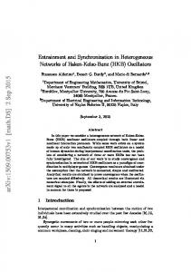
Fig. 1. Two layer network architecture.
The WSN structure used here consists of two layers – WSN node layer and GW layer, depicted in Fig. 1. The lines between the nodes indicate communication links; red nodes are elected Cluster Sinks (CS). WSN nodes are arranged in clusters, as this approach can ensure increased energy efficiency, routing and easier network scaling. Within the scope of this paper we are not interested in how clusters are formed or how cluster head is elected, but we know that all sensor nodes are homogeneous, meaning, they have the same hardware and software running on them. The second, GW layer, is formed again from homogeneous gateway nodes, and again hardware and software here is the same on each and every node. As seen in Fig. 1, communication link is possible between 1) cluster nodes and the cluster sink (CS), 2) CS and available GW or GWs, 3) between cluster heads only by using GW as proxy, 4) between GWs themselves, 5) between GWs and the user. We assume that GWs can always communicate with each other. D. Assumptions and Limitations So far there are some assumptions of synchronization approach we can devise from the presented information: 1) Network route from the sensor node to the user is quite simple, because, at minimum, there are only three communication hops to reach the user; 2) From network architecture we can easily obtain the synchronization hierarchy and constructing it does not involve separate algorithms or steps, meaning that the lower level node synchronizes to a higher layer node – GW synchronizes to, for example, NTP server or other time provider; CS to GW and Cluster Nodes (CN) to CS; 3) Due to GW position being sporadic, not always cluster heads can have access to the external network. So the GWs must employ mechanism that can synchronize clusters in multi‒hop manner; 4) Cluster N is covered by at least one GW – on its own ensuring all node or in our case cluster coverage is a
57
Technologies of Computer Control 2014 / 15 ______________________________________________________________________________________________ separate problem in WSNs and is included as a future research topic. In [4] it is pointed out that there are several limitations that should be taken into account when choosing or devising the synchronization scheme. Namely, this adds to the following aspects of limitations: Energy efficiency: Synchronization should not drastically increase energy consumption; Scalability: As the sensor node count increases/decreases the synchronization should not be affected by changes in topology; Precision: Depending on application some may need microsecond accuracy while others may just require the ordering of events; Robustness: Synchronization scheme should be robust against the link and node failures. For this purpose, usually, more than needed sensor nodes are deployed in a relatively small area; Lifetime: Here it is decided whether the synchronization is needed for an instant, or for the entire lifetime of the network; Scope: The scope decides whether the nodes are synchronized network wide or locally, among nodes that are spatially close; Cost: What costs are incurred while deploying the scheme. Since the sensor networks are often deployed in remote areas, it is better not to rely on sophisticated hardware infrastructures like GPS receivers. Rather, an internal synchronization is enough if implemented appropriately. E. Synchronization Problems and Errors Achieving synchronization is not an easy task because due to the following non-deterministic delay is introduced [1] and [4]: 1) Send Time. The time spent to assemble a packet and to send it to the MAC layer. This time includes kernel processing and the delay introduced by the operating system, if there is one; 2) Access Time. This is the time loss experienced while waiting to access the transmission channel. It depends on the specific MAC protocol used; 3) Transmission Time. The time the sender spends to transmit the packet bit by bit. Influenced by baud rate and packet size; 4) Propagation Time. The time needed for the packet to be transmitted from the sender to the receiver. It is the physical propagation time of the packet through the media channel and this is small enough in most cases to be ignored from latency estimations; 5) Receive Time. The time the receiver takes to receive and to process the packet. Clock skew rate [4] (or drift [3] and clock offset are the things that change over time and they must be corrected whenever synchronization is executed. Due to the mentioned time this problem is not that easily resolved. Furthermore, such resources as available energy, wireless communication medium and computational power limit the implementation of reliable synchronization approach. Another aspect is network dynamics – due to limited resources nodes
58
can often be removed from the network or added thus changing topology, or nodes can even be mobile; this could affect approaches that use, for example, spanning trees (like LTS) or other non-Ad-Hoc network topology [3]. III. CLOCK SYNCHRONIZATION APPROACH In this chapter we try to describe a simple enough time synchronization approach that could be used for time synchronizing in the two layered mobile GW network. For node pair synchronization we want to use simple roundtrip timestamp communication like in TPSN [4], which is based on the timestamp exchange among nodes, but as described later, with slight modifications. We chose to base on these methods, because there has been wide research on these methods and it is proven that they can guarantee good enough (according to [3] average uncertainty of timestamp intervals is described as 200 µs and it changes by 2.5 µs with every second passed) precision with little overhead. From what we described previously we know that the following features will be implemented: 1) Simple network hierarchy – SN, CS, GW, user; 2) Four different communication links: SN – CS (P2P); CS – GW (P2P); GW – GW (Ad-Hoc); GW – user (P2P); 3) GW ability to synchronize without access to external network; 4) At least one GW has access to external network; 5) To minimize access time uncertainty nodes will be in priority mode when communicating, so that it does not have to wait on other nodes. Now we have clear concept of network architecture that will be used and the features that result from the used network architecture. We have decided that the best approach is to do synchronization in several separate, but successive steps: 1) GW synchronization with global time; 2) CSs synchronization with GW; 3) CNs synchronization with CS. A. Gateway Synchronization to Global Time Here we can see two different cases. First, in the network only one GW has access to external network. Second, several GWs have access to external network. In the first case everything is clear – the GW that has access to external network will be the source of synchronization time and all clusters and every other GW will synchronize to this GW. To synchronize to global time a simple NTP synchronization will be used. In the second case to begin the synchronization process correctly first of all master GW must be chosen among GWs and then the same approach as in the first case can be executed. Possible problems or sources of errors: the main problem with this step is latency, propagation of time among GWs take time. To resolve this problem we use separate network (Wi-Fi for example) to synchronize GWs and WSN network (at the same time) to synchronize to the cluster. This insures that GWs receive time as soon as some neighbour has received it. If the application is developed for use in wild there exists a possibility to equip every node with GPS receiver and then
Technologies of Computer Control ______________________________________________________________________________________________ 2014 / 15 synchronizing with global time is not a relevant problem. After reading global time from the GPS module every GW is synchronized with global time and furthermore between themselves. We assume that the time difference between different GPS receivers is negligible. Possible problems or sources of errors: While using GPS, the received data processing time has to be included. As described in [6] this time can vary from 50 ms to 100 ms and more if pulse per second (PPS) synchronization is not used on GPS module. Alternatively this timebound can be a few microseconds. To supplement this case we must mention that GPS is not a necessary module, though. Synchronization source can be a simple node that can access the external network, where the time is acquired, like it was described in the beginning of this subsection. Another possibility to reduce the cost of external communication is to maintain local time, meaning that GWs do not synchronize to global time by using the methods just described. In this case the master GW should be chosen and all GWs should synchronize to this GW time. Drawback: synchronization to global time must be done later (posteriori) when data is sent to the user; this could lead to uncertainties of when some events have happened. Furthermore, some message roundtrip synchronization algorithm must be used because there is no dedicated hardware (as BSD would need) and this could lead to further error in lower hierarchy levels because every next hop in hierarchy increases uncertainty as described in [3]. B. Cluster Sink Synchronization to Gateway Time Initially CSs are unsynchronized with GWs and are running on some local time TL while GW is now running on global time TG. As soon as GW has received global time and synchronized to all its neighbouring GWs – it is necessary to forward TG further in the network. After which GW responds to CS sent SYNC_REQ message. Synchronization here is similar to what happens in TPSN. First GW sets priority so synchronization with this CS node could be performed uninterrupted and informs every neighbouring node of this. After receiving SYNC_REQ, GW replies with ACK, containing T1. At ACK message reception timestamp T2 is measured. After some time response message is sent measuring timestamps T3 and T4. Finally the last timestamp message from GW is sent to CS measuring timestamps T5 and T6. This is a slight modification of TPSN protocol where one more additional message is inserted. This is done in hope to minimize the time offset that is introduced due to message transmission in GW. Furthermore, receiving one more message is not as expensive as sending one.
So now we can calculate the time offset like this: ∆=
|
(𝑇2−𝑇1)+(𝑇6−𝑇5) |−|𝑇4−𝑇3| 2
2
'
(1)
where T1, T2, T3, T4, T5 and T6 are timestamps that are exchanged among synchronization partners and ∆ is average time difference between communication partners. TCS now is calculated as: 𝑇𝐶𝑆 = 𝑇5 + |∆| + 𝑡calculation,
(2)
where T5 is the last received global time timestamp from GW, ∆ is average time difference between communication partners and tcalculation is time that is spent to process all received data from the moment the last message was received. Here with three messages we try to achieve better time offset measurement. But this must be tested or simulated to verify our assumptions. C. Cluster Node Synchronization to Cluster Sink When CS is synchronized with GWs, further synchronization to SN can be performed. We know few facts about sensor nodes, namely, they are divided in clusters and one CH is elected, thus providing one hop route to every cluster node. Cluster is homogeneous and nodes have limited resources. Here the same synchronization approach as between GW and CS will be performed. D. Resynchronization Due to the instabilities of clock source and other environmental factors clock and therefore time drifts away from its time. To resynchronize we use the following mechanism – after some time has passed, there are methods how to calculate it – we perform resynchronization, depicted in Fig. 3. Resynchronization is described by 𝑇𝐶𝑆 = 𝑇1 + |∆| + 𝑡calculation ,
(3)
where ∆ is known from the synchronization which was the second time after the calculated time of needed resynchronization and T1 is GWs timestamp and tcalaculation is time of message processing. For this approach to work, nodes must be static, because with change of location ∆ will change as well. GW
T1
RESYNC_REQ ACK CS T2 Fig. 3. Resynchronization process. Fig. 2. Timestamp exchange process.
59
Technologies of Computer Control 2014 / 15 ______________________________________________________________________________________________ BEGIN SYNC_START: IF GW is a master (has access to external network) THEN GW receives global time trough NTP ELSE IF Master GW not elected THEN Perform election of master GW GOTO SYNC_START ELSE IF Synchronization started THEN Wait for global time IF Global time received THEN
Fig. 5. After two steps all neighbors are synchronized.
GOTO CHECK_NEIGHBOURS: CHECK_NEIGHBOURS: IF GW has any neighbour GW left unsynchronized THEN Perform synchronization with neighbour GW GOTO CHECK_NEIGHBOURS ELSE GOTO SYNC_TO_CLUSTER SYNC_TO_CLUSTER: IF GW has unsynchronized CS THEN Perform synchronization to this CS GOTO SYNC_TO_CLUSTER ELSE GW - CS synchronization done GOTO SYNC_TO_NODE;
Fig. 6. After the 3rd step one more GW is synchronized and the first GW starts cluster head synchronization.
SYNC_TO_NODE: IF CS has unsynchronized nodes THEN Perform synchronization to this node GOTO SYNC_TO_NODE ELSE CS - node synchronization done GOTO END; END Pseudo-code 1. Pseudo‒code that illustrates network‒wide synchronization process.
A. Network-wide Synchronization To illustrate more in detail the network‒wide synchronization we present Pseudo‒code 1 and Figs. 4 ‒ 8 that describe how all network synchronization is acquired. In Figs. 4 ‒ 8. for depiction simplicity only GW and CS synchronization process is shown. Pseudo-code 1 can be visualized with the help of the following example of the two layered, clustered sensor network:
Fig. 7. After the 4th step one more GW is synchronized and the first cluster has synchronized its second cluster head and two more clusters have started synchronization with cluster sinks.
And so forth until all the nodes are synchronized.
Fig. 8. After the 11th step all GWs and cluster heads have been synchronized.
To sum up the usage of the two layer network architecture we can quite easily provide sensor node synchronization to global time in a few easily implementable phases. Fig. 4. Initial state of network after electing master GW.
60
Technologies of Computer Control ______________________________________________________________________________________________ 2014 / 15 IV. FUTURE WORK The biggest issue that we came across is providing actual synchronization results from experiments or simulations for the provided approach. So we are working on creating both a simulation setup in Omnet++ (Castalia) and a simple test bed for result comparison. For the test bed we will be using DiGi Wi-9C board (or Raspberry PI) as GW and for the sensor nodes TI eZ430-RF2500 sensor nodes. Besides simulation there is one more interesting case to be researched – when two or more separate partitions working on the same application need to be synchronized. We need to find a reliable way to do this. V. CONCLUSION In this paper we have suggested the time synchronization approach that is implemented in two layer network. The first layer is formed from clustered sensor nodes and the second layer is formed from mobile gateways. The proposed time synchronization approach starts working from top – master gateway, to bottom – sensor node, step by step. Basic approaches used for synchronization are based on the packet delay measurement. The advantage of the proposed synchronization system is that different parts of network can perform synchronization separately. The greatest disadvantage of this paper is that due to time limitation we did not manage to provide the data to prove the efficiency of the proposed approach. REFERENCES [1]
[2]
[3]
[4]
X. Liu, S. Zhou, “Evaluation of Several Time Synchronization Protocols in WSN,” 2010 International Conference of Information Science and Management Engineering, Aug. 2010, pp. 488–491. http://dx.doi.org/10.1109/ISME.2010.222 A. Ageev, D. Macii, A. Flammini, “Towards an adaptive synchronization policy for wireless sensor networks,” 2008 IEEE International Symposium on Precision Clock Synchronization for Measurement, Control and Communication, Sep. 2008, pp. 115–120. http://dx.doi.org/10.1109/ISPCS.2008.4659224 R. Kay, P. Blum, L. Meier, “Time Synchronization and Calibration in Wireless Sensor Networks,” Handbook of Sensor Networks: Algorithms and Architectures, 2005. V. Singh, S. Sharma, T. P. Sharma, “Time Synchronization in WSN: A survey,” International Journal of Enhanced Research in Science Technology & Engineering, 2013, vol. 2, no. 5, pp. 61–67.
G. Miezitis, V. Zagurskis, R. Taranovs, “Multiple Mobile Gateways in Wireless Sensor Networks,” Scientific Journal of RTU, Computer Science, vol. 13, 2012, pp. 38–42. [6] Lammert Bies, “Time synchronization with a Garmin GPS,” [Online]. [Accessed: 31 July 2014]. Available from: http://www.lammertbies.nl/ comm/info/GPS-time.html [7] NTP internet time servers at linocomm.net [Online]. [Accessed: 13 Aug. 2014]. Available from: http://ntp.linocomm.net/index.en.html [8] H. Karl, A. Willig, Protocols and Architectures for Wireless Sensor Networks, John Wiley & Sons, p. 526, 2005. [9] I. Demirkol, C. Ersoy, F. Alagoz, “MAC Protocols for Wireless Sensor Networks: A Survey,” IEEE Press, 2006, pp. 115–121. [10] T. Laukkarinen, J. Suhonen, M. Hännikäinen, “A Survey of Wireless Sensor Network Abstraction for Application Development,” International Journal of Distributed Sensor Networks, 2012, 12 p., Article ID 740268. http://dx.doi.org/10.1155/2012/740268 [11] D. Mills, “Network Time Protocol (Version 3) Specification, Implementation and Analysis” RFC Editor, 1992. [12] H. Weibel, “The Second Edition of the High Precision Clock Synchronization Protocol,” Zurich University of Applied Sciences: Technology Update on IEEE 1588, Embedded World, Nürnberg, Mar. 3–5, 2009. [5]
Gundars Miezitis was born in 1987. Master degree in computer science (Riga Technical University, 2012). Now he is a PhD student at Riga Technical University, Institute of Computer Control, Automation and Computer Science, Department of Computer Networks and System Technology. Currently he is working at Riga Technical University. Previous work includes research connected with Wireless Sensor Network localization problems and localization using radio signal strength. Email:
[email protected] Romans Taranovs had received B. S. as well as Mg. sc. ing. degree in Computer Science from Riga Technical University in 2007 and 2009 respectively. In 2014 he has received Ph.D in Computer Science at Riga Technical University. Now he is an assistant at Computer Networks and System Technology department of RTU. As well as he is a development lead at Accenture. His research interests are self-organizing wireless sensor networks, embedded systems and cloud computing. R. Taranov is an IEEE Student member since 2010. He has been involved in EU project Stratos and several Latvian Council of Science projects. Email:
[email protected] Valerijs Zagurskis, received his M. S. in computer science in 1965 from Riga Technical University (RTU) and his Candidate of technical science (Ph. D) in circuits and systems in 1972 from Latvian Academy of Science, Doctor of Technical Science in 1990 in Ukrainian Academy of Science and Dr. habil. sc. comp. in 1992 in Latvian University. He is a professor at RTU and head of department of Computer networks and systems technology (DTSTK), as well as a member of the IEEE and ACM an expert in the Latvian Council of Science. His research interests include networks, mixed signal system design, MAC protocols, resource scheduling, cross-layer design, and cooperative functioning of systems, wireless ad hoc and sensor networks. Email:
[email protected]
Gundars Miezītis, Romāns Taranovs, Valērijs Zagurskis. Klasteros sadalīta heterogēna bezvadu sensoru tīkla inicializācija Bezvadu sensoru tīkla mezglu sinhronizācija ir viena no funkcionalitātēm, kas dod vairākas jaunas iespējas bezvadu sensoru tīklam. Piemēram, bezvadu sensoru tīklā var izmantot algoritmus, kuri darbojas tikai tad, ja ir zināms sistēmas laiks starp mezgliem. Viena no tādām algoritmu klasēm ir vides piekļuves algoritmi, balstīti uz TDMA – Time Division Multiple Access ideju, kad katram mezglam tiek piešķirts konkrēts laika slots, kurā tas klausās vidi un veic komunikāciju, pārējā laikā mezgls atrodas miega režīmā. Ja šāda iespēja nebūtu, tad mezglam vide būtu jāklausās nepārtraukti un lieki tiktu tērēti tam pieejamie enerģijas resursi. Cits piemērs, ja sensoru tīkls izpilda kādu laika grafiku, piemēram, sensoru tīklam ir jādarbojas naktī vai dienā, visprecīzākais veids, kā to realizēt, ir veikt laika sinhronizāciju uz mezgliem un iegūt globālo laiku. Piemēram, situācijā, kad tiktu izmantoti apgaismojuma sensori, atbilde par to, vai ir diena vai nakts, nav viennozīmīgi – dienā var būt aptumšota istaba un sensors var pieņemt aplamu lēmumu, ka ir nakts, un sākt nevajadzīgi tērēt savus resursus. Piedāvātā pieeja izmanto tā saucamo laika zīmogu nodošanas mehānismu, kad sūtītājs un saņēmējs apmainās ar šiem laika zīmogiem un saņēmējs izrēķina, par cik tad viņa laiks atšķiras no globālā laika. Kad tas ir izrēķināts, šis mezgls sev uzstāda jau koriģēto vērtību. Ja mezgls, kurš darbojās, ir vārteja vai klastera galva, tad tiek pārbaudīts, vai visi kaimiņu mezgli ir sinhronizēti, izmantojot atbildes ziņojumus – ja netiek saņemta atbilde, ka vajag sākt sinhronizāciju, tad kādā noteiktā laikā tiek pieņemts, ka visi kaimiņu mezgli ir sinhronizēti. Tālāk jau uz mezgla var sākt izpildīties vai nu pielietojums, vai kāds cits inicializācijas solis. Šīs darbības ir identiskas gan uz vārtejas, gan uz klastera galvas. Tiek piedāvāts arī paņēmiens, kā veikt atkārtotu mezglu sinhronizāciju, jo takts avota neprecizitātes un vides apstākļu ietekmes dēļ sinhronizācija tiek zaudēta. Šeit uz mezgla tiek saglabāta tā vērtība, kas ir bijusi izrēķināta iepriekšējā sinhronizācijas ciklā, kas ir ticis izpildīts pēc laika, kas tiek uzskatīts par sinhronizācijas punkta zaudēšanu. Šī pieeja dažādām tīkla daļām dod iespēju sinhronizēties neatkarīgi vienai no otras.
61
Technologies of Computer Control 2014 / 15 ______________________________________________________________________________________________ Гундарс Миезитис, Валерий Загурский, Роман Таранов. Синхронизация узлов в беспроводных сенсорных сетях с гетерогенной кластерной архитектурой. Синхронизация беспроводных сенсорных узлов является функциональностью, которая позволяет реализовать ряд новых возможностей в беспроводной сенсорной сети. Например, может быть упомянута возможность беспроводной сенсорной сети использовать алгоритмы, которые основываются на отсчёте времени в узлах системы. К примеру, алгоритмы TDMA типа,основанные на множественном доступе к среде с разделением времени. В данном случае за каждым узлом закрепляется конкретный временной интервал, в котором он слушает среду и общается, а в течение остальной части времени находится, к примеру, в спящем режиме. Алгоритмы данного типа позволяют эффективно расходовать энергоресурсы сенсорных узлов – иначе, к примеру, узлы должны будут слушать среду постоянно, что приведёт к более быстрой трате имеющихся энергоресурсов. Другой пример, где сенсорная сеть работает по графику – такая сенсорная сеть должна работать в дневное или вечернее время. Самым точным способом для составления и выполнения графика является использование синхронизации узлов, основанной на глобальном времени. В таких сетях использование дополнительного оборудования для определения времени суток не является решением, поскольку существуют ситуации, когда, к примеру, при использовании фотоэлементов может быть дан ложный ответ – комната, где установлены сенсорные узлы, может быть затемнена искусственно. Предлагаемый подход использует так называемые временные маркеры. При их помощи приёмник и передатчик вычисляют, на сколько локальное время приёмника отличается от глобального. После того, как данное различие было рассчитано, узел сам регулирует значение локального таймера. Если узел является шлюзом или основой кластера, алгоритм обеспечивает проверку все соседних сенсорных узлов, с помощью ответных сообщений. Если не будет получено никакого ответа, что нужно начать синхронизацию, предполагается, что все соседние узлы синхронизированы. Далее на узлах могут начинать работать либо другие шаги инициализации, либо само приложение. Эти действия являются идентичными для узлов типа шлюз и глава кластера. В работе также предложен метод для повторной синхронизации узлов, поскольку из-за неточности источника тактовой частоты и из-за условий окружающей среды синхронизации теряется. Этот подход позволяет синхронизировать различные части сенсорной сети независимо друг от друга.
62