Acta Geophysica DOI: 10.2478/s11600-014-0218-5
Noise Reduction in Radon Monitoring Data Using Kalman Filter and Application of Results in Earthquake Precursory Process Research Mojtaba NAMVARAN1 and Ali NEGARESTANI2 1
Kerman Graduate University of Technology, Geophysics Department, Kerman, Iran; e-mail:
[email protected] (corresponding author) 2 Kerman Graduate University of Technology, Electrical Engineering Department, Kerman, Iran; e-mail:
[email protected]
Abstract Monitoring the concentration of radon gas is an established method for geophysical analyses and research, particularly in earthquake studies. A continuous radon monitoring station was implemented in Jooshan hotspring, Kerman province, south east Iran. The location was carefully chosen as a widely reported earthquake-prone zone. A common issue during monitoring of radon gas concentration is the possibility of noise disturbance by different environmental and instrumental parameters. A systematic mathematical analysis aiming at reducing such noises from data is reported here; for the first time, the Kalman filter (KF) has been used for radon gas concentration monitoring. The filtering is incorporated based on several seismic parameters of the area under study. A novel anomaly defined as “radon concentration spike crossing” is also introduced and successfully used in the study. Furthermore, for the first time, a mathematical pattern of a relationship between the radius of potential precursory phenomena and the distance between epicenter and the monitoring station is reported and statistically analyzed. Key words: radon anomaly, Kalman filter (KF), noise reduction, effective precursory (EP) ratio, seismic activity.
________________________________________________ © 2014 Institute of Geophysics, Polish Academy of Sciences
M. NAMVARAN and A. NEGARESTANI
1.
INTRODUCTION
The devastations (both financial losses and casualties) caused by frequent and high-magnitude earthquakes in Iran necessitate scientific studies for understanding the geophysical activities in this country. The Kerman province located in south east Iran is one of the most seismically active regions in Iran and the Middle East. This is caused by an influence of stress field that results from convergence and collision between the Arabia and Eurasia plates (Berberian et al. 2001). Concentration of the active faults with the northnorth western (N-NW) to south-south eastern (S-SE) trend indicates stressreservoir in this region (Berberian et al. 1984). The Golbaf and Shahdad (located in Kerman province) right lateral strike-slip faults with the N-S trend have raised expectation about seismic reservoir-triggering in this area (Berberian et al. 1984). Over the past few decades, some parts of these faults have developed their seismic activities. According to the catalogue by Iranian Seismological Center (IRSC) and International Institute of Earthquake Engineering and Seismology (IIEES), this earthquake-prone region has experienced more than 15 seismic events with M6.0 and higher in the last seven decades (IRSC & IIEES earthquake database). The radon monitoring in soil and groundwater is a useful tool to study the possible link between the variations in radon concentration and deformation phenomena due to tectonic activities (Ramola 2010, Seyis et al. 2010, Hashemi et al. 2013). An increasing or decreasing radon concentration before earthquake is apparently caused by movements deep within the earth, following stress, loading and rupture of rocks (Hauksson 1981). So, crustal radon-flux measurement along active faults can provide useful information about movements in micro-fractures of the crust. Decreases in radon concentration were registered, for instance, before the following earthquakes: Japan 1984-1988 (Wakita et al. 1991), Taiwan 2008 (Kuo et al. 2006), Turkey 2009-2010 (Ali Yalım et al. 2012). In order to distinguish between the variations of radon concentration caused by earthquakes from those caused by other sources, different studies have been reported (Negarestani et al. 2002, Richon et al. 2004, Ali Yalım et al. 2012). Prior to performing any investigation in the field, it is necessary to perform a pre-processing analysis on data to reduce noise (Finkelstein et al. 1998). This enhances the reliability of data for pattern recognition between data parameters. A detailed survey was carried out to decide on a reliable noise reduction mechanism that would reflect the complexities of radon gas behavior (Finkelstein et al. 1998). Kalman filter (KF) was found to be a very reliable and yet novel approach for radon gas monitoring studies (Simon 2001). So, it has been successfully employed and the results are reported
RADON MONITORING DATA AND KALMAN FILTER
here. The Kalman filter is an analytical model frequently used for state estimation in state space models (SSM) when the standard Gaussian noise assumption does not apply (Simon and Chia 2002). The linear state space model postulates that an observed time series is a linear function of a state vector and the law of motion for the state vector is first-order vector autoregression (AR) (Simon and Chia 2002). In recent years, KF has become a very powerful, intelligent and computational tool widely used in signal processing applications such as noise reduction (Brailean et al. 1995, Fujimoto and Ariki 2000, Evensen 2003, Brabec and Jílek 2007). The main advantage of this approach is designing an efficient filter to control noisy systems. In other words, the basic idea of a KF is producing less noisy data from a full noisy data. According to KF algorithm, it removes noises by assuming a pre-defined model of a system (Kleinbauer 2004). This means that KF is employed to remove the noises which are mixed with signals during the measurement. A continuous radon monitoring station for groundwater gas monitoring was set up in Jooshan hot-spring. After few months of monitoring, some anomalies in low concentration of radon could be observed. Hence, alongside the investigation of radon gas concentration, the objectives of this article were set to be: to reduce commonly observed noises on radon time-series data, using KF, to define the anomaly shape and discuss a relation between filtered data and seismic parameters, and to find a correlation between radon decreasing rate and seismic parameters. 2.
EXPERIMENTAL PROCEDURE
Initially, a continuous monitoring of radon gas concentration was performed in Jooshan hot-spring complex situated near Jooshan village in Kerman province. The site location was carefully chosen: it is located between the two active faults Golbaf and Shahdad. The monitoring period was done in a seismically active season of the region from December 2011 to April 2012. The main device used in this study is a RAD7 detector coupled with a measuring toolbox. The measured air is sucked from the water container using an air pump into the trap, then into the detector. The RAD7 radon monitor (DURRIDGE Company Inc., USA) is a commercial model, widely used in many applications involving continuous radon activities measurement. The detector counts the number of α-disintegrations into its chamber during a specified time (in this study it was 10 minutes). The Kalman filter was then developed for noise reduction in the process. As this is an analytical model, like in any modeling study some assumption need to be made. Very careful considerations were made to make the re-
M. NAMVARAN and A. NEGARESTANI
quired assumptions so that they would reflect the complexities of radon gas monitoring data in the closest and most realistic way. The KF model was then incorporated on the observational results using a commercial MATLAB® package, to analyze the noise reduction effect. 3.
THEORETICAL HYPOTHESIS
3.1 Dobrovolsky equation Dobrovolsky et al. (1979) suggested a theoretical-empirical relationship between size of the effective precursor manifestation zone and the main earthquake magnitude as: D = 100.43 M ,
(1)
where M is the magnitude of the earthquake, and D is the effective radius of earthquake [km] called “strain radius”. This equation was developed for estimating the deformation and tilts in surface of the earth as a magnitude function of the coming earthquake and distance from the epicenter. In other words, geochemical signals can only be caused by earthquakes with epicentral distances less than or equal to this empirical “magnitude-epicentral distance” relation (Dobrovolsky et al. 1979). 3.2 State space model 3.2.1 Non-linear SSM State space model (SSM) refers to a class of probabilistic graphical models
that describe the probabilistic dependence between the latent state variable (x) and the observed measurement (z) (Kleinbauer 2004). In other words, SSM is a mathematical simulation of a process, where the state of process is represented by a numerical vector. The state or the measurement can be either continuous or discrete. SSM is subdivided into two separate models (Simon 2001): the process model, which describes how the state propagates in time in response to the external influences (for example input and noise), and the measurement model, which describes how measurements (z) are taken from the process, typically simulating noisy and/or inaccurate measurement which could occur due to different reasons. The most general from of an SSM is the non-linear state. The two main function of non-linear SSM are: xt +1 = f ( xt , ut , wt ) ,
(2)
zt = h ( xt , vt ) ,
(3)
RADON MONITORING DATA AND KALMAN FILTER
Fig. 1. Fundamentals of the state space model (SSM). Notice: z–1 is z-transform in digital signal processing which governs unit delay function.
where f and h functions govern state propagation (x) and measurements (z), respectively, u is the process input, w and v are state and measurement noise vectors, respectively, and t is the discrete time. Functions f and h are usually based upon a set of discretized differential equations, governing the dynamics and observations during the process. Fundamentals of SSM are illustrated in Fig. 1. 3.2.2 Linear state space model (LSSM) Suppose that a multiple parallel time series are observable in a process. Usually, the source series of interest are not directly measureable, but hidden in them. In addition, the mixing system generating the observable series from the source is unknown. For simplicity, the mixing system is assumed linear. The aim is to recover these sources, as well as to model their dynamics (Roesser 1975). This is referred to as blind source separation (BSS) (Cichocki and Amari 2002). A matrix as A is assumed, which is the transfer function between sources and signal receivers. Most array processing techniques rely on the modeling of A: each column of A is assumed to depend on a small number of parameters. This information may be provided either by physical modeling or by direct array calibration. BSS consists in identifying A and/or retrieving the source signals without resorting to any a priori information about mixing matrix A; it exploits only the information carried by the received signals themselves, hence, the term “blind” (Cichocki and Amari 2002). According to literature, statistical independence has played a great role in BSS; in most BSS algorithms the sources are assumed to be statistically independent (Belouchrani et al. 1997, Lee et al. 1999, Zibulevsky and Pearlmutter 2001). In the noiseless case, certain techniques have been proposed to solve this problem efficiently (Zhang and Hyvärinen 2011). For example, if the sources are non-Gaussian or at most one of them is Gaussian, BSS can be solved (Hyvärinen and Oja 2000). As it is explained in the following sections, the recorded data in this study showed the Gaussian distribution. Therefore, the above description could be applied to them (Fig. 2).
M. NAMVARAN and A. NEGARESTANI
Fig. 2. Gaussian statistical distribution of radon gas concentration and its Gaussian fit. According to the distribution of this kind, BSS can be solved by the independent component analysis technique for these data.
Fig. 3. Fundamentals of linear state space model (LSSM). This linear model is easier both to calculate and analyze.
Considering Fig. 3, an LSSM is a model where functions f and h are linear in both state and input. The functions can then be described by using the matrices P, Q, and R, reducing the state propagation calculations to linear algebra. Hence, the SSM would follow (Kleinbauer 2004): xt +1 = Pt xt + Qt ut + wt ,
(4)
zt = Rt xt + vt .
(5)
RADON MONITORING DATA AND KALMAN FILTER
This linear model is easier both to calculate and analyze and also enables investigating properties such as control-ability, observability, and frequency response. 3.3 A random walk process When faced with a time series that shows irregular growth, the best strategy may not be to try to directly predict the level of the series at each period (i.e., the quantity yt). Instead, it may be better to try to predict the change that occurs from one period to the next (i.e., the quantity yt – yt–1). In other words, it may be helpful to look at the first difference of the series, to see if a predictable pattern can be discerned there (Simon 2001, Spitzer 2001). For practical purposes, it is just as good to predict the next change as to predict the next level of the series, since the predicted change can always be added to the current level to yield a predicted level (Kleinbauer 2004, Spitzer 2001). Hence, the forecasting model suggested in this description is yt − yt −1 = α ,
(6)
where α is the mean of the first difference, i.e., the average change from one period to the next. If we rearrange this equation to put yt by itself on the left, we get yt = yt −1 + α .
(7)
In other words, we predict that this period’s value will equal the last period’s value plus a constant representing the average change between periods (Spitzer 2001). This is the so-called “random walk” model. It assumes that, from one period to the next, the original time series merely takes a random step away from its last recorded position (Spitzer 2001). According to the above description, a random walk is defined as a process where the current value of a variable is composed of the past value plus an error term known as “white noise” (ε). White noise is a random signal with a flat power spectral density and is called white because it affects all the frequency components of a signal equally (Spitzer 2001). Random walk is thereby analytically represented as: yt = yt −1 + ε t .
(8)
The implication of a process of this type is that the best prediction of y for next period is the current value, or in other words the process does not allow predicting the change (yt – yt–1). That is, the change of y is absolutely random. It can be shown that the mean of a random walk process is constant but its variance is not. Therefore, a random walk process is non-stationary, and its variance increases with discrete time (t).
M. NAMVARAN and A. NEGARESTANI
Considering the radon migration to follow random walk, this mechanism is used to model radon diffusion and migration through the earth crust. The soil – as a radon propagation medium prior to monitoring – is represented by a system of randomly oriented baffles. The mean distance d over which the atom travels between two collisions takes on the role of a mean free path. The effective mean time between two collisions, or in other words the migration time/orientation/velocity, is strongly random and depends on medium sectional properties, such as temperature, humidity, porosity, permeability of soil, etc. 3.4 Kalman filter The KF is a recursive predictive filter which is based on the use of statespace technique and recursive algorithms. This filter estimates the state of a “dynamic system”. This dynamic system can be disturbed by noise of different kind, mostly assumed as white noise (white noise is a random signal with a flat power spectral density) (Kleinbauer 2004). To upgrade the estimated state, the KF uses measurements that are related to the state but disturbed as well (Simon and Chia 2002). Overall, the KF consists of two stages, prediction and correction. In the first stage, the state of the system is predicted with the dynamic model. In the second stage, the state of the system is corrected with the observation model. Thereby, it minimizes the error covariance of the estimator. The KF is called as a recursive filter; because the procedure of the system is repeated for each time step with the state of the previous time step as initial value (Fig. 4).
Fig. 4. Circuit of the Kalman filter. This procedure is repeated for each time step with the state of the previous time step as initial value. Therefore, the KF is called a recursive filter (Kleinbauer 2004).
RADON MONITORING DATA AND KALMAN FILTER
The state vector includes the variables of interest and describes the state of the dynamic system and also suggests its degree of freedom (Brabec and Jílek 2007). The variables in the state vectors can be inferred from values that are measurable (Kleinbauer 2004). In other words, they cannot be measured directly. State vectors contain two different values at the same time. These are the predicted value before the update (a priori value) and the corrected value after the update (a posteriori value) (Kleinbauer 2004). The time update equations are responsible for projecting forward (in time) using the current state and error covariance estimates to obtain the a priori estimates for the next time step (Kleinbauer 2004). An important point regarding the state vector is its transformation over time, which is known as a dynamic model. Another term that should be described here is “observation model”. This model illustrates the significant relation between the state and the measurement. In scientific terms, the KF estimates the state of a linear system. In order to design and implement a KF, an estimate of the process variables is required. Furthermore, in order to design a KF to eliminate noise from a signal, the process of measuring must be describable as a linear phenomenon. 3.5 KF model for tracking applications According to above descriptions, monitoring of radon during diffusion/ migration is an exact example of random walk. Each monitored sample consists of two parts; a real value that indicates the released radon from the earth plus a white noise which is produced due to the effect of environmental parameter on radon concentration and/or measurement process. According to several publications, the original predict-update KF equations for tracking applications of a linear system, as assumed for our case, are as below (Cichocki and Amari 2002, Kleinbauer 2004, Leśniak et al. 2009): Predict xˆt |t −1 = Ft xˆt −1|t −1 + Bt ut ,
(9)
Pt |t −1 = Ft Pt −1|t −1 Ft T + Qt .
(10)
Update
(
)
xˆt |t = xˆt |t −1 + K t yt − H t xˆt |t −1 ,
(
K t = Pt |t −1 H tT H t Pt |t −1 H tT + Rt Pt |t = ( I − K t H t ) Pt |t −1 ,
)
−1
(11) ,
(12) (13)
M. NAMVARAN and A. NEGARESTANI
where xˆ is the estimated state, F the state transition matrix, u the control variables, B the control matrix, P the state variance matrix (i.e., error of estimation), Q the process variance matrix (i.e., error due to process), y the measurement variables, H the measurement matrix, K the Kalman gain, R the measurement variance matrix (i.e., error from measurement), and the subscripts are as follows: (t|t) the current time period, (t–1|t–1) the previous time period, and (t|t–1) the intermediate steps. All variants are designated according to their appearance: Normal (a) denotes scalars, and bold-italic (a) denotes vectors. According to the above explanations, the KF eliminates noise by assuming a pre-defined model for a system. Obviously, such a model must be reliable. In order to satisfy the reliability criteria for the model, the following stages are considered during development of any such model (so considered in this study): model the state process, model the measurement process, model the noise (this needs to be done for both the state and measurement process), test the filter, refine the filter. 4.
PROPOSED KF MODEL FOR RADON CONCENTRATION MONITORING
In this Section, we are trying to estimate the level of radon released from the earth during the experiment. The measurements obtained are from the RAD7-device outputs. As explained, monitoring of radon during diffusion/migration is an exact example of random walk. Each monitored sample consists of two parts: a real value that indicates the released radon from the earth, plus a white noise which is produced due to effect of environmental parameters on radon concentration and/or measurement process. On the other hand, as explained in the following section, the data recorded in this study showed Gaussian distribution, facilitating the BSS analysis. Considering the above, a KF model is developed here to estimate the level of radon gas released during the experiments. Generally, the concentration of radon in the earth could be: increasing, decreasing or static (i.e., the level of radon concentration could be varied prior to an earthquake); sloshing or stagnant (i.e., the relative level of radon to the average level is changing over time, or is static). The simplified scheme of the modeled system is given in Fig. 5.
RADON MONITORING DATA AND KALMAN FILTER
Fig. 5. A schematic plan of radon level behind the monitoring station. The level of radon can be varied (increased, decreased or static) by different phenomena, especially before earthquakes.
As per any modeling or simulation, some assumptions are required to be made. Such assumptions should not broadly affect the reliability or the reallife situation of the process. On the other hand, no investigations on using the KF model for radon gas monitoring have been reported in the literature. So, a simple yet reliable benchmark KF model for radon gas monitoring is developed. The following assumptions and formulizations are considered: the level of released radon is considered to be constant (i.e., L = C); the predict-update equations would then be reduced to scalar (i.e., xˆ = x where x is the estimate of L); also, for the constant model, xt +1 = xt , so Ft = 1 for any t ≥ 0; also in this case, control variables, B and u, are not used; also, the level of radon concentration is represented by y = y. the scale of measurement (z) and state estimate (x) are the same; therefore H = 1; noise is assumed to be from the measurement, so R = r; the process is scalar; therefore P = p. the noise is also considered as Q = q.
Considering the above, the predict-update equations can be rewritten as: Predict: x(t⎮t −1) = x(t −1⎮t −1) ,
(14)
P(t⎮t −1) = P(t −1⎮t −1) + q(t ) .
(15)
Update: Kt =
P(t⎮t −1) P(t⎮t −1) + r(t )
,
(16)
M. NAMVARAN and A. NEGARESTANI
(
)
x(t⎮t ) = x(t⎮t −1) + K(t ) * y(t ) − x(t⎮t −1) ,
(
(17)
)
P(t⎮t ) = 1 − K(t ) * P(t⎮t −1) .
(18)
The KF filter is now completely modeled. Initially, the state progress is considered to be an arbitrary number, with an extremely high variance as it is completely unknown: x0 = 0 and P0 = 1000. It is worth noting that the START
x(0,0) = 0, q = 1, P(0,0) = 1000, t = 1 m = number of inputs
Data (y(t)) ± Noise (R(t))
x(t,t–1) = x(t–1,t–1) P(t,t–1) = P(t–1,t–1) + q K(t) = P(t,t–1) (P(t,t–1) + r(t))–1
t=t+1
X(t,t) = x(t,t–1) + K(t) (y(t) – x(t,t–1)) P(t,t) = (1 – K(t)) P(t,t–1)
t=m
YES
NO END
Fig. 6. The algorithm of proposed Kalman filter. Based on the state equation, the data has been read and filtered in each step and the next value has been read as initial value.
RADON MONITORING DATA AND KALMAN FILTER
more realistic the variable is the faster the convergence of the model would be. The system noise is assumed to be q = 1, because the systematic error of the measurement device (RAD7) is exactly 1 Bq/m3 (according to RAD7 instruction catalogue). The proposed filter could then be illustrated schematically as Fig. 6. 5.
RESULTS AND DISCUSSION
During the monitoring of radon concentration in Jooshan hot-spring (December 2011 to April 2012) more than 35 seismic events with different
Fig. 7. Seismic activity during the study period (from December 2011 until April 2012) in study area. During this period, more than 35 events with different magnitudes occurred in the 100 km radius around the station. Colour version of this figure is available in electronic edition only.
M. NAMVARAN and A. NEGARESTANI
magnitudes were recorded in a radius span of 100 km around the station. Figure 7 indicates the seismicity of regions around Golbaf and Shahdad faults during the study period. In this study, the effective precursory (EP) ratio is introduced and applied as: EP = D / R ,
(19)
where D [km] is calculated from Eq. 1 and R [km] is the distance from the epicenters of each earthquake to the monitoring station. The calculated value of EP indicates the ability of each seismic event to be used as a precursor. The higher EP means the larger magnitude earthquake and closer epicenters to the monitoring station. Summary of all seismic events with M ≥ 2.5 during the study and their effective precursory ratio is given in Table 1. All the seismic data and their relevant parameters (e.g., epicenter, magnitude, and depth) are taken from IRSC and IIEES catalogues. In order to narrow down the data to a handful and reliable number of inputs, the events with EP ≥ 0.4 were used for the KF model analysis. Table 1 The parameters of reported earthquakes in vicinity of the monitoring station during the study period* Date 29 Dec 2011 05 Jan 2012 06 Jan 2012 09 Jan 2012 09 Jan 2012 09 Jan 2012 13 Jan 2012 17 Jan 2012 28 Jan 2012 05 Feb 2012 10 Feb 2012 15 Feb 2012 17 Feb 2012 21 Feb 2012 23 Feb 2012 24 Feb 2012 27 Feb 2012
Local time 20:40 23:00 03:41 08:59 12:56 14:08 05:06 02:06 13:32 11:55 14:11 18:57 04:26 08:58 07:59 04:51 18:48
Lat.
Long.
29.9 30.5 29.9 30.1 29.9 29.9 29.2 30.1 30.2 30.6 30.1 32.0 29.8 29.8 30.4 30.0 31.4
57.8 57.5 57.7 57.6 57.6 57.7 58.1 57.2 57.4 57.1 57.6 58.5 57.6 57.3 57.4 57.5 56.7
Depth MagniD [km] tude 10.1 2.5 11.8 5.0 2.9 17.6 6.1 3.0 19.4 7.9 3.3 26.2 10.2 2.7 14.4 10.1 2.6 13.1 13.5 3.7 38.9 12.2 2.8 15.9 6.1 3.2 23.7 10.0 3.1 21.5 6.2 2.7 14.4 5.4 4.3 70.6 15.5 2.5 11.8 6.1 3.2 23.7 5.1 2.9 17.6 10.2 2.7 14.4 10.4 5.4 209.8
*)The source of seismic data: IRSC (with permission).
R [km] 35.2 39.4 23.1 3.9 18.2 26.8 115.1 41.8 21.9 70.7 4.1 230.9 30.7 46.7 37.5 12.6 163.7
EP 0.33 0.44 0.83 6.71 0.79 0.48 0.33 0.38 1.08 0.30 3.51 0.30 0.38 0.50 0.46 1.14 1.28
RADON MONITORING DATA AND KALMAN FILTER
5.1 Noise reduction Statistical distribution of the monitored level of radon gas concentration and its Gaussian fit are given in Fig. 2. As reported in statistical papers for such distributions, BSS can be solved by the independent component analysis technique (Evensen 2003, Kownacki 2011). In different studies, it has been reported that the deviations exceeding ±1, ±1.5, and ±2 σ from the average concentration level are considered as anomalies, and thereby potentially linked to the geodynamics of the area. Zmazek et al. (2005) proposed the ± σ threshold approach for anomaly descriptions. Summary of the thresholds and the associated type of anomalies of this approach are given in Table 2. According to this approach, in ±1 σ group, 57% of anomalies is correct and related to seismic events (CA), 38% of them appeared without seismic events (FA), and finally in 5% cases no anomaly is observed for an earthquake (NA) (Zmazek et al. 2005). On the other hand, in the ±2 σ group, 50, 27, and 22% of anomalies are CA, FA, and NA, respectively (Zmazek et al. 2005). Thereby, for this study, the ±1 σ threshold is selected to investigate the relation of the filtered data with geodynamics events. Table 2 Different thresholds and the associated anomaly in ±σ approach (Zmazek et al. 2005) Anomaly CA FA NA
±1.0 σ 12 8 1
±1.5 σ 10 8 3
±2.0 σ 9 5 4
Note: CA refers to radon concentration anomalies correct and related to seismic activity, NA refers to those anomalies caused by sources other than seismic activity, and FA refers to nonactive period.
A commercial version of MATLAB® is used to evaluate and analyze the monitored results alongside the noise reduction data (incorporating the developed KF filter). A summary of the data analysis is given in Fig. 8. A comparison of monitored data before and after filtering is given in Fig. 8A. The differences between these two curves (before and after noise reduction) are proportional to the measurement system (RAD7) noise (q). It can be seen that the filtered signal is much smoother than the monitored data. This can be explained, as in the spectral analysis it is reported that the KF model decreases the high frequency components of the recorded signal. It also shows the reliability of the filtered data for further investigations. The magnitudes of earthquakes and the EP ratio of the seismic activities are pro-
M. NAMVARAN and A. NEGARESTANI
Fig. 8: (A) Measured radon signal and filtered radon signal, (B) magnitude of earthquakes that occurred during the measurement period, and (C) effective precursory (EP) ratio for each earthquake. Colour version of this figure is available in electronic edition only.
vided in Fig. 8B and C, respectively; all are in the same time span (together with Fig. 8A, covering the whole period of study. From Fig. 8, it is clear that there is good correlation between sharp anomalies and earthquake occurrence. As can be observed, in a few hours to a few days prior to an earthquake, a variation in radon level is visible. Figure 9 illustrates the variation of radon gas concentration during the monitoring period, after applying the KF filter. As can be seen, the overall number of sudden changes (A-V) was 22. These are investigated in further details to realize their potential relationship to the reported earthquakes. In this time series signal, the average and standard deviation of data are 82214.18 and 16776.92, respectively. So, the values of x + σ , x − σ , x + 2σ , and x − 2σ are inferable, which are 98991.10, 65437.26, 115768.02, and 48660.34, respectively. Point A is not a real peak in radon concentration, but it is due to the operation of KF. The KF initialized the process of filtering with an arbitrary number with an ex-
RADON MONITORING DATA AND KALMAN FILTER
Fig. 9. Filtered signal whose all peaks have been labeled. The values of average (black), x̄ + σ (green), x̄ – σ (yellow), x̄ + 2σ (red), and x̄ – 2σ (violet) have been drawn. The sharp increase in the initial part of signal (point A) is due to the operation of KF. Colour version of this figure is available in electronic edition only.
tremely high variance, as it is completely unknown. The value of variance controls the velocity of convergence. It means that initializing with a more meaningful variable results in faster convergence. Among the A-V labeled peaks, only a few provide good correlation with the reported seismic events. These are categorized in 7 different ranges and labeled as (I-VIII) in Fig. 9. For instance, 53 hours after the recorded peak F (categorized in the range I), an earthquake with M3.3 and an EP value of 6.71 occurred. By comparison to the unfiltered data (Fig. 8A) this sudden variation in radon concentration is also obvious. This event was about 4 kilometers away from the monitoring station, with radon activity crossing the σ level above the average value. Point M (range III) in Fig. 9 shows the bottom of a sharp decrease. This happened between sample numbers 3174 and 3477 and prolonged for 50 hours. During this period, the level of radon concentration decreased from 96 kBq/m3 down to 60 kBq/m3 (minimum point) and then started to increase. About 92 hours after this peak, an earthquake M3.2 with EP = 1.08 occurred. The location of the earthquake was about 22 kilometers away from the Jooshan hot-spring. Peak P (Fig. 9 – just after range IV), occurred after a sharp decrease in level of radon concentration monitored in sample 4048. This decrease started from 3929 sample until 4048 samples and then started increasing toward the normal value. An earthquake M2.7 with EP = 3.51 occurred about 4 kilometers away from the station, 105 hours after this peak. During this fluctuation, the level of radon declined from 101 to 71 kBq/m3 at the minimum state and then started to increase. According to the above description of data fluctuations, an anomaly is introduced as “radon concentration spike crossing”:
M. NAMVARAN and A. NEGARESTANI
RS = x ± σ ,
(20)
where x is the average value of measured values, and σ is the standard deviation. As described, all earthquakes happened after the x ± σ threshold line in filtered data and these points illustrate anomalous behavior in radon signal. Among the ranges in Fig. 9, there are few ranges in which the radon concentration behaved anomaly but no earthquake occurred after these behaviors. This suggests the uncertainties involved with the Dobrovolsky equation and its need to be modified. 5.2 Pattern recognition Another important result of this study is recognizing the pattern of relation between filtered radon concentration signal and the EP ratio. As explained in Fig. 8A, the filtered data is smoother than the measured data. Thereby, the rate of variation in filtered radon concentration is introduced to be changed by the angle of the decreasing line, which we denote as θ. As illustrated in Fig. 10, between points E to F, θ = 90°. After this stage, an event M3.3 with EP = 6.71 occurred. Also, between points J to K, L to M, O to P, and Q to R, the decreasing angles are 79°, 88°, 84°, and 81°, respectively. After these anomalies, seismic events occurred with M3.2, M2.7, M2.7, and M5.4, respectively. Therefore, θ could be described as the rate of variation in radon level. In other words, the higher slope of radon signal after noise cancelation indicates that the fluctuation is sharper, and vice versa. Different studies, e.g., Wakita et al. (1991), Kuo et al. (2006), and Tsunomori and Kuo (2010) suggest that the level of radon concentrated in soil and groundwater decreases from background levels to a lower level prior an earthquake and then
Fig. 10. Decreasing angles of radon signal (θ). Different values of θ could describe the rate of variation in radon level. In this study, θ has been in good correlated with EP ratio.
RADON MONITORING DATA AND KALMAN FILTER
Fig. 11. The decline angles before earthquake (θ) plotted as a function of EP ratio.
starts to increase before reaching its previous normal value. Based on this, in order to describe the correlation between θ and EP, values of decreasing angles before earthquakes were plotted as a function of EP ratio (Fig. 11). Therefore, the equation of the best straight fit-line of the figure would be EP = α + βθ ,
(21)
where EP is the effective precursory ratio (Eq. 19), θ is the decreasing angle (degree) on the filtered radon concentration data, β is the slope of straight fitline, and α is determined by points values. Also the correlation coefficient r2 was determined to be 0.78, indicating that θ and EP ratio were correlated to each other. Based on previous descriptions and the proposed pattern, it is concluded here that the probability of an earthquake occurrence increases proportional to the increased value of θ. 6.
CONCLUSION
A continuous radon concentration monitoring analysis was performed at the widely reported earthquake-prone area of Jooshan hot-spring (located near Golbaf and Shahdad faults), Kerman province, south east Iran. Analytical analysis using Kalman filter modeling on noise reduction from the radon concentration signal was reported for the first time. The main scientific conclusions of the study are as summarized here: During the measurement, parameters of different kind result in noises on signals. So, before interpreting the data, the effects of these noises must be reduced as much as possible.
M. NAMVARAN and A. NEGARESTANI
KF is a powerful tool which is successfully reported to decrease the highfrequency components of the recorded signal of the monitored radon gas concentration. A novel threshold on the filtered radon concentration data is defined as “radon concentration spike crossing” beyond which a seismic event seems inevitable. Occasionally, anomalies were observed on the radon concentration figure but no seismic events were reported. This suggests uncertainties involved with the Dobrovolsky equation. A new ratio between the effective radius (as proposed by Dobrovolsky) and the distance of the earthquake from the monitoring station was defined as “effective precursory” ratio. This proved a much better understanding of the mechanism of the radon concentration signal. The use of KF filter also facilitated much detailed analytical analysis of data. From the filtered data, a decreasing angle was reported to have proportional effect on the possibility of forthcoming earthquake. Effective precursory (EP) ratio and the decreasing angles were found to be remarkably correlated. Generally, the level of radon concentration was found to be a useful measure as a precursor, few hours to few days prior to an earthquake. The delay time between the anomalies and seismic event depends on different parameters such as geological features of case study, environmental parameters, etc. Therefore, in order to increase the reliability of the findings on precursory role of radon concentration level, it can be useful to increase the number of stations and duration of measurement in future analyzes.
A c k n o w l e d g e m e n t . The authors are extremely grateful to the International Center for Science and Technology and Environmental Sciences (ICST) for permission to use RAD7 detector and other instruments of Earthquake Precursors lab. We are so grateful to Dr. Reza Negarestani for reviewing the paper, Mr. Seyyed Hadi Hosseini and Mr. Mohsen Dezvareh for their help in plotting figures and also Dr. Majid Shahpasandzadeh, Dr. Ali Esmaeily, Dr. Seyyed Mohammad Musavi Nasab, Mr. Habibollah Montazeri, and Mr. Morteza HajEbrahimi for their kind guidance. All the seismic data are reported by permission from earthquake catalogue of the Iranian Seismological Center (IRSC) and International Institute of Earthquake Engineering and Seismology (IIEES). In seismic observatory instrumentation all the standards suggested by World Wide Standard Seismograph Network (WWSSN) are taken into account.
RADON MONITORING DATA AND KALMAN FILTER
References Ali Yalım, H., A. Sandıkcıoğlu, O. Ertuğrul, and A. Yıldız (2012), Determination of the relationship between radon anomalies and earthquakes in well waters on the Akşehir-Simav Fault System in Afyonkarahisar province, Turkey, J. Environ. Radioactiv. 110, 7-12, DOI: 10.1016/j.jenvrad.2012.01.015. Belouchrani, A., K. Abed-Meraim, J.-F. Cardoso, and E. Moulines (1997), A blind source separation technique using second-order statistics, IEEE Trans. Signal Process. 45, 2, 434-444, DOI: 10.1109/78.554307. Berberian, M., J.A. Jackson, M. Ghorashi, and M.H. Kadjar (1984), Field and teleseismic observations of the 1981 Golbaf–Sirch earthquakes in SE Iran, Geophys. J. Roy. Astr. Soc. 77, 3, 809-838, DOI: 10.1111/j.1365-246X. 1984.tb02223.x. Berberian, M., J.A. Jackson, E. Fielding, B.E. Parsons, K. Priestley, M. Qorashi, M. Talebian, R. Walker, T.J. Wright, and C. Baker (2001), The 1998 March 14 Fandoqa earthquake (Mw 6.6) in Kerman province, southeast Iran: Re‐rupture of the 1981 Sirch earthquake fault, triggering of slip on adjacent thrusts and the active tectonics of the Gowk fault zone, Geophys. J. Int. 146, 2, 371-398, DOI: 10.1046/j.1365-246x.2001.01459.x. Brabec, M., and K. Jílek (2007), State-space dynamic model for estimation of radon entry rate, based on Kalman filtering, J. Environ. Radioactiv. 98, 3, 285297, DOI: 10.1016/j.jenvrad.2007.05.006. Brailean, J.C., R.P. Kleihorst, S. Efstratiadis, A.K. Katsaggelos, and R.L. Lagendijk (1995), Noise reduction filters for dynamic image sequences: a review, Proc. IEEE 83, 9, 1272-1292, DOI: 10.1109/5.406412. Cichocki, A., and S.-I. Amari (2002), Adaptive Blind Signal and Image Processing. Learning Algorithms and Applications, John Wiley & Sons, Chichester. Dobrovolsky, I.P., S.I. Zubkov, and V.I. Miachkin (1979), Estimation of the size of earthquake preparation zones, Pure Appl. Geophys. 117, 5, 1025-1044, DOI: 10.1007/BF00876083. Evensen, G. (2003), The Ensemble Kalman Filter: theoretical formulation and practical implementation, Ocean Dynam. 53, 4, 343-367, DOI: 10.1007/ s10236-003-0036-9. Finkelstein, M., S. Brenner, L. Eppelbaum, and E. Ne’Eman (1998), Identification of anomalous radon concentrations due to geodynamic processes by elimination of Rn variations caused by other factors, Geophys. J. Int. 133, 2, 407-412, DOI: 10.1046/j.1365-246X.1998.00502.x. Fujimoto, M., and Y.Ariki (2000), Noisy speech recognition using noise reduction method based on Kalman filter. In: Proc. IEEE Int. Conf. on Acoustics, Speech, and Signal Processing, ICASSP’2000, 5-9 June 2000, Istanbul, Turkey, Vol. 3, 1727-1730, DOI: 10.1109/icassp. 2000.862085. Hashemi, S.M., A. Negarestani, M. Namvaran, and S.M. Musavi Nasab (2013), An analytical algorithm for designing radon monitoring network to predict the
M. NAMVARAN and A. NEGARESTANI
location and magnitude of earthquakes, J. Radioanal. Nucl. Chem. 295, 3, 2249-2262, DOI: 10.1007/s10967-012-2310-0. Hauksson, E. (1981), Radon content of groundwater as an earthquake precursor: Evaluation of worldwide data and physical basis, J. Geophys. Res. 86, B10, 9397-9410, DOI: 10.1029/JB086iB10p09397. Hyvärinen, A., and E. Oja (2000), Independent component analysis: algorithms and applications, Neural Networks 13, 4-5, 411-430, DOI: 10.1016/S0893-6080 (00)00026-5. Kleinbauer, R. (2004), Kalman filtering implementation with Matlab, Study Report, Universität Stuttgart, Institute of Geodesy. Kownacki, C. (2011), Optimization approach to adapt Kalman filters for the realtime application of accelerometer and gyroscope signals’ filtering, Digit. Signal Process. 21, 1, 131-140, DOI: 10.1016/j.dsp.2010.09.001. Kuo, T., K. Fan, H. Kuochen, Y. Han, H. Chu, and Y. Lee (2006), Anomalous decrease in groundwater radon before the Taiwan M6.8 Chengkung earthquake, J. Environ. Radioactiv. 88, 1, 101-106, DOI: 10.1016/ j.jenvrad.2006.01.005. Lee, T.-W., M.S. Lewicki, M. Girolami, and T.J. Sejnowski (1999), Blind source separation of more sources than mixtures using overcomplete representations, IEEE Signal Process. Lett. 6, 4, 87-90, DOI: 10.1109/ 97.752062. Leśniak, A., T. Danek, and M. Wojdyła (2009), Application of Kalman filter to noise reduction in multichannel data, Schedae Informaticae 17, 18, 63-73, DOI: 10.2478/v10149-010-0004-3. Negarestani, A., S. Setayeshi, M. Ghannadi-Maragheh, and B. Akashe (2002), Layered neural networks based analysis of radon concentration and environmental parameters in earthquake prediction, J. Environ. Radioactiv. 62, 3, 225-233, DOI: 10.1016/S0265-931X(01)00165-5. Ramola, R.C. (2010), Relation between spring water radon anomalies and seismic activity in Garhwal Himalaya, Acta Geophys. 58, 5, 814-827, DOI: 10.2478/s11600-009-0047-0. Richon, P., F. Perrier, J.-C. Sabroux, M. Trique, C. Ferry, V. Voisin, and E. Pili (2004), Spatial and time variations of radon-222 concentration in the atmosphere of a dead-end horizontal tunnel, J. Environ. Radioactiv. 78, 2, 179-198, DOI: 10.1016/j.jenvrad.2004.05.001. Roesser, R.P. (1975), A discrete state-space model for linear image processing, IEEE Trans. Automat. Contr. 20, 1, 1-10, DOI: 10.1109/tac.1975.1100844. Seyis, C., S. İnan, and T. Streil (2010), Ground and indoor radon measurements in a geothermal area, Acta Geophys. 58, 5, 939-946, DOI: 10.2478/s11600-0100012-y. Simon, D. (2001), Kalman filtering, Embedded Sys. Program. 14, 6, 72-79.
RADON MONITORING DATA AND KALMAN FILTER
Simon, D., and T.L. Chia (2002), Kalman filtering with state equality constraints, IEEE Trans. Aero. Elec. Sys. 38, 1, 128-136, DOI: 10.1109/7.993234. Spitzer, F. (2001), Principles of Random Walk, 2nd ed., Graduate Texts in Mathematics, Vol. 34, Springer, New York. Tsunomori, F., and T. Kuo (2010), A mechanism for radon decline prior to the 1978 Izu-Oshima-Kinkai earthquake in Japan, Radiat. Meas. 45, 1, 139-142, DOI: 10.1016/j.radmeas.2009.08.003. Wakita, H., G. Igarashi, and K. Notsu (1991), An anomalous radon decrease in groundwater prior to an M6.0 earthquake: A possible precursor?, Geophys. Res. Lett. 18, 4, 629-632, DOI: 10.1029/91GL00824. Zhang, K., and A. Hyvärinen (2011), A general linear non-Gaussian state-space model: Identifiability, identification, and applications. In: C.-N. Hsu and W.S. Lee (eds.), JMLR Workshop and Conference Proc., Asian Conf. on Machine Learning 2011, Tokyo, Japan, 113-128. Zibulevsky, M., and B.A. Pearlmutter (2001), Blind source separation by sparse decomposition in a signal dictionary, Neural Comput. 13, 4, 863-882, DOI: 10.1162/089976601300014385. Zmazek, B., M. Živčić, L. Todorovski, S. Džeroski, J. Vaupotič, and I. Kobal (2005), Radon in soil gas: How to identify anomalies caused by earthquakes, Appl. Geochem. 20 6, 1106-1119, DOI: 10.1016/j.apgeochem. 2005.01.014. Received 1 January 2013 Received in revised form 10 December 2013 Accepted 23 December 2013