Nov 15, 2016 - N° 456. January 2015. Project-Team Socrate. Noisy Channel-Output. Feedback Capacity of the. Linear Deterministic. Interference Channel.
TECHNICAL REPORT N° 456 January 2015 Project-Team Socrate
ISRN INRIA/RT--456--FR+ENG
Victor Quintero, Samir M. Perlaza, Jean-Marie Gorce
ISSN 0249-0803
arXiv:1608.08920v2 [cs.IT] 15 Nov 2016
Noisy Channel-Output Feedback Capacity of the Linear Deterministic Interference Channel
Noisy Channel-Output Feedback Capacity of the Linear Deterministic Interference Channel Victor Quintero, Samir M. Perlaza, Jean-Marie Gorce Project-Team Socrate Technical Report n° 456 — January 2015 — 34 pages Abstract: In this technical report, the capacity region of the two-user linear deterministic (LD) interference channel with noisy output feedback (IC-NOF) is fully characterized. This result allows the identification of several asymmetric scenarios in which implementing channel-output feedback in only one of the transmitter-receiver pairs is as beneficial as implementing it in both links, in terms of achievable individual rate and sum-rate improvements w.r.t. the case without feedback. In other scenarios, the use of channel-output feedback in any of the transmitter-receiver pairs benefits only one of the two pairs in terms of achievable individual rate improvements or simply, it turns out to be useless, i.e., the capacity regions with and without feedback turn out to be identical even in the full absence of noise in the feedback links. Key-words: Capacity, Linear Deterministic Interference Channel, Noisy Channel-Output Feedback
Victor Quintero, Samir M. Perlaza and Jean-Marie Gorce are with the CITI Laboratory of the Institut National de Recherche en Informatique et en Automatique (INRIA), Université de Lyon, and Institut National de Sciences Apliquées (INSA) de Lyon. 6 Av. des Arts 69621 Villeurbanne, France. ({victor.quintero-florez, samir.perlaza, jean-marie.gorce}@inria.fr). Victor Quintero is also with Universidad del Cauca, Popayán, Colombia. Samir M. Perlaza is also with the Department of Electrical Engineering at Princeton University, Princeton, NJ. This research was supported in part by the European Commission under Marie Sklodowska-Curie Individual Fellowship No. 659316 (CYBERNETS); and the Administrative Department of Science, Technology, and Innovation of Colombia (Colciencias), fellowship No. 617-2013. Parts of this work were presented at the IEEE International Workshop on Information Theory (ITW), Jeju Island, South Korea, October, 2015. This work was also submitted to the IEEE Transactions on Information Theory in November 10 2016.
RESEARCH CENTRE GRENOBLE – RHÔNE-ALPES
Inovallée 655 avenue de l’Europe Montbonnot 38334 Saint Ismier Cedex
Capacité du Canal Linéaire Déterministe à Interférences avec Rétroalimentation Degradée par Bruit Additif. Résumé : Dans ce rapport, la région de capacité du canal linéaire déterministe à interférences avec rétroalimentation degradée entre les récepteurs et leurs émetteurs correspondants est caractérisée. Ce résultat permet l’identification de plusieurs scenarios asymétriques dans lesquels la rétroalimentation dans un seul couple récepteur-émetteur montre autant de bénéfices que des rétroalimentations dans les deux couples récepteurs-émetteurs. Ces bénéfices sont mis en évidence par l’amélioration des taux de transmission individuels et de leur somme par rapport aux cas où il n’y a aucune rétroalimentation. D’autres scenarios montrent qu’une rétroalimentation dans un des couple émetteur-récepteur améliore le taux individuel d’un des deux couples émetteurs-récepteurs. D’ailleurs, il existe d’autres scenarios où l’utilisation d’un ou plusieurs liens de rétroalimentation ne montre aucun bénéfice ni pour les taux individuels ni pour leur somme. Dans ces scenarios, cela montre que les régions de capacité avec et sans rétroalimentation sont identiques. Mots-clés : Région de Capacité, Modèle linéaire déterministe, canal à interférences, rétroalimentation degradée.
Noisy Channel-Output Feedback Capacity of the Linear Deterministic Interference Channel
3
Contents 1 Notation
4
2 Problem Formulation
4
3 Main Results
6
4 Conclusions
12
Appendices
17
A Proof of Achievability
17
B Proof of Converse
26
RT n° 456
Noisy Channel-Output Feedback Capacity of the Linear Deterministic Interference Channel
1
4
Notation
Throughout this technical report, sets are denoted with uppercase calligraphic letters, e.g. X . Random variables are denoted by uppercase letters, e.g., X. The realizations and the set of events from which the random variable X takes values are respectively denoted by x and X . The probability distribution of X over the set X is denoted PX . Whenever a second random variable Y is involved, PX Y and PY |X denote respectively the joint probability distribution of (X, Y ) and the conditional probability distribution of Y given X. Let N be a fixed natural number. An N dimensional vector of random variables is denoted by X = (X1 , X2 , ..., XN )T and a corresponding realization is denoted by x = (x1 , x2 , ..., xN )T ∈ X N . Given X = (X1 , X2 , ..., XN )T and (a, b) ∈ N2 , with a < b 6 N , the (b − a + 1)-dimensional vector of random variables formed by the components a to b of X is denoted by X(a:b) = (Xa , Xa+1 , . . . , Xb )T . The notation (·)+ denotes the positive part operator, i.e., (·)+ = max(·, 0) and EX [·] denotes the expectation with respect to the distribution of the random variable X. The logarithm function log is assumed to be base 2.
2
Problem Formulation
Consider the two-user linear deterministic interference channel with noisy channel-output feedback (LD-IC-NOF) described in Figure 1. For all i ∈ {1, 2}, with j ∈ {1, 2} \ {i}, the number − of bit-pipes between transmitter i and its corresponding intended receiver is denoted by → n ii ; the number of bit-pipes between transmitter i and its corresponding non-intended receiver is denoted by nji ; and the number of bit-pipes between receiver i and its corresponding transmitter − . These six integer non-negative parameters fully describe the LD-IC-NOF in is denoted by ← n ii Figure 1. At transmitter i, the channel-input X i,n at channel use n, with n ∈ {1, 2, . . . , N }, is a qÄ (1) (2) ä (q) T dimensional binary vector X i,n = Xi,n , Xi,n , . . . , Xi,n , with − − q = max (→ n 11 , → n 22 , n12 , n21 ) , (1) → − and N the block-length. At receiver i, the channel-output Y i,n at channel use n is also a qÄ→ → − − (1) → − (2) → − (q) äT dimensional binary vector Y i,n = Y i,n , Y i,n , . . . , Y i,n . The input-output relation during channel use n is given by → − → − Y i,n =S q− n ii X i,n + S q−nij X j,n , (2) ← − and the feedback signal Y i,n available at transmitter i at the end of channel use n satisfies: Å ã → − ← − +− ← −T T → (0, . . . , 0) , Y i,n =S (max( n ii ,nij )− n ii ) Y i,n−d , (3) where d is a finite delay, additions and multiplications are defined over the binary field, and S is a q × q lower shift matrix of the form: 0 0 0 ··· 0 1 0 0 ··· 0 .. 0 ··· . S= 0 1 (4) . . . . .. .. ... 0 .. 0 ··· 0 1 0 RT n° 456
Noisy Channel-Output Feedback Capacity of the Linear Deterministic Interference Channel
(1)
n21
! n 11
1
1
X1,n
(2) X1,n
2
2
X1,n
(3) X1,n
3
3
X1,n
(3)
X2,n
4
4
(4) X1,n
(2) X2,n
5
5
(5)
X2,n
(5) X1,n
(1)
X2,n (2)
X2,n
! n 22
(3)
X2,n (4)
X2,n (5) X2,n
(2)
RX1
T X1
n12
(1)
X1,n
(4) X1,n
X1,n
n 11 (1)
(3)
(1)
X1,n
1
1
2
2
X2,n
(1)
X1,n
3
3
X2,n
(2)
X1,n
4
4
X2,n
(3)
X1,n
5
5
(4)
X1,n
RX2
T X2
Signal
Interference
5
X2,n
(2)
(3)
n 22
(4)
(5)
Feedback
Figure 1: Two-user linear deterministic interference channel with noisy channel-output feedback at channel use n. � ← − − , max(→ − The dimension of the vector (0, . . . , 0) in (3) is q − min ← n n ii , nij ) and the vector Y i,n ii � → − ← − +− → − , max(→ − represents the min ← n n ii , nij ) least significant bits of S (max( n ii ,nij )− n ii ) Y i,n−d . ii Without any loss of generality, the feedback delay is assumed to be equal to 1 channel use, i.e., d = 1. Transmitter i sends the message index Wi by sending the codeword X i = (X i,1 , X i,2 , . . . , X i,N ) ∈ (1) Xiq×N . The encoder of transmitter i can be modeled as a set of deterministic mappings fi , (2) (N ) (1) (n) fi , . . ., fi , with fi : Wi → {0, 1}q and for all n ∈ {2, 3, . . . , N }, fi : Wi × {0, 1}q(n−1) → {0, 1}q , such that � (1) X i,1 =fi Wi and (5) � ← − ← − ← − (n) (6) X i,n =fi Wi , Y i,1 , Y i,2 , . . . , Y i,n−1 . Let T ∈ N be fixed. Assume that during a given communication, T blocks are transmitted. T Hence, the decoder of receiver i is defined by a deterministic Äfunction ψi : {0, 1}q×N ×T ä → Wi . → − → − → − At the end of the communication, receiver i uses the sequence Y i,1 , Y i,2 , . . . , Y i,N T to obtain an estimate of the message indices: Ä (1) ä Ä− ä → − → − c ,W c (2) , . . . , W c (T ) =ψi → W Y i,1 , Y i,2 , . . . , Y i,N T , i
(t)
i
i
(7)
c is an estimate of the message index sent during block t ∈ {1, 2, . . . , T }. The decoding where W i (t) error probability in the two-user G-IC-NOF during block t, denoted by Pe (N ), is given by Å ã Å ã! (t) (t) (t) (t) (t) ”1 6= W ”2 6= W Pe (N )=max Pr W , Pr W . (8) 1 2 RT n° 456
Noisy Channel-Output Feedback Capacity of the Linear Deterministic Interference Channel
6
The definition of an achievable rate pair (R1 , R2 ) ∈ R2+ is given below. Definition 1 (Achievable Rate Pairs) A rate pair (R1 , R2 ) ∈ R2+ is achievable if there exists at least one pair of codebooks X1N and X2N with codewords of length N , and the corresponding (1) (2) (N ) (1) (2) (N ) encoding functions f1 , f1 , . . . , f1 and f2 , f2 , . . . , f2 such that the decoding error prob(t) ability Pe (N ) can be made arbitrarily small by letting the block-length N grow to infinity, for all blocks t ∈ {1, 2, . . . , T }. The following section determines the set of all the rate pairs (R1 , R2 ) that are achievable in the − − − and ← − . LD-IC-NOF with parameters → n 11 , → n 22 , n12 , n21 , ← n n 11 22
3
Main Results
− − − ,← − Denote by C(→ n 11 , → n 22 , n12 , n21 , ← n 11 n 22 ) the capacity region of the LD-IC-NOF with para→ − → − ← − ← − meters n 11 , n 22 , n12 , n21 , n 11 , and n 22 . Theorem 1 fully characterizes this capacity region. − − − ,← − Theorem 1 The capacity region C(→ n 11 , → n 22 , n12 , n21 , ← n 11 n 22 ) of the two-user LD-IC-NOF is the set of non-negative rate pairs (R1 , R2 ) that satisfy for all i ∈ {1, 2}, with j ∈ {1, 2} \ {i}: − − 6min (max (→ n ii , nji ) , max (→ n , n )) , (9a) ää Ä Ä ii ij + → − → − ← − → − , (9b) Ri 6min max ( n ii , nji ) , max n ii , n jj − ( n jj − nji ) ä Ä + + → − → − → − → − R1 + R2 6min max ( n 22 , n12 ) + ( n 11 − n12 ) , max ( n 11 , n21 ) + ( n 22 − n21 ) , (9c) � � + − − − − )+ R1 + R2 6max (→ n 11 − n12 ) , n21 , → n 11 − (max (→ n 11 , n12 ) − ← n 11 � � + → − → − → − ← − )+ , + max ( n 22 − n21 ) , n12 , n 22 − (max ( n 22 , n21 ) − n (9d) 22 Ri
+ − − 2Ri + Rj 6max (→ n ii , nji ) + (→ n ii − nij ) � � + − − − − )+ . + max (→ n jj − nji ) , nij , → n jj − (max (→ n jj , nji ) − ← n jj
(9e)
The proof of Theorem 1 is divided into two parts. The first part describes the achievable region and is presented in Appendix A. The second part describes the converse region and is presented in Appendix B. Theorem 1 generalizes previous results regarding the capacity region of the LD-IC with channel− = 0 and ← − = 0, Theorem 1 describes the caoutput feedback. For instance, when ← n n 11 22 − > max (→ − pacity region of the LD-IC without feedback (Lemma 4 in [1]); when ← n n 11 , n12 ) 11 ← − → − and n 22 > max ( n 22 , n21 ), Theorem 1 describes the capacity region of the LD-IC with perfect − − − = ← − , channel output feedback (Corollary 1 in [2]); when → n 11 = → n 22 , n12 = n21 and ← n n 11 22 Theorem 1 describes the capacity region of the symmetric LD-IC with noisy channel output − − feedback (Theorem 1 in [3] and Theorem 4.1, case 1001 in [4]); and when → n 11 = → n 22 , n12 = n21 , ← − → − ← − n ii > max ( n ii , nij ) and n jj = 0, with i ∈ {1, 2} and j ∈ {1, 2} \ {i}, Theorem 1 describes the capacity region of the symmetric LD-IC with only one perfect channel output feedback (Theorem 4.1, cases 1000 and 0001 in [4]).
Comments on the Achievability Scheme The achievable region is obtained using a coding scheme that combines classical tools such as rate splitting, superposition coding, and backward decoding. This coding scheme is described in Appendix A. In the following, an intuitive description of this coding scheme is presented. RT n° 456
Noisy Channel-Output Feedback Capacity of the Linear Deterministic Interference Channel
7
(t)
Let the message index sent by transmitter i during the t-th block be denoted by Wi ∈ (t) {1, 2, . . . , 2N Ri }. Following a rate-splitting argument, assume that Wi is represented by three (t) (t) (t) subindices (Wi,C1 , Wi,C2 , Wi,P ) ∈ {1, 2, . . . , 2N Ri,C1 } × {1, 2, . . . , 2N Ri,C2 } × {1, 2, . . . , 2N Ri,P }, (t)
(t)
(t)
where Ri,C1 + Ri,C2 + Ri,P = Ri . The codeword generation from (Wi,C1 , Wi,C2 , Wi,P ) follows (t−1)
a four-level superposition coding scheme. The index Wi,C1 is assumed to be decoded at transmitter j via the feedback link of transmitter-receiver pair j at the end of the transmission of block t − 1. Therefore, at the beginning of block t, each transmitter possesses the knowledge (t−1) (t−1) (0) of the indices W1,C1 and W2,C1 . In the case of the first block t = 1, the indices W1,C1 and (0)
W2,C1 correspond to two indices assumed to be known by all transmitters and receivers. Using these indices both transmitters are able to identify the same codeword in the first code-layer. N (R1,C1 +R2,C1 ) This code-layer codewords (see Figure 15). Denote by Ä first ä is a sub-codebook of 2 (t−1) (t−1) u W1,C1 , W2,C1 the corresponding codeword in the first code-layer. The second codeword (t)
is chosen by transmitter i using Wi,C1 from the second code-layer, which is a sub-codebook Ä (t−1) ä (t−1) of 2N Ri,C1 codewords corresponding at u W1,C1 , W2,C1 as shown in Figure 15. Denote by Ä (t−1) ä (t−1) (t) ui W1,C1 , W2,C1 , Wi,C1 the corresponding codeword in the second code-layer. The third code(t)
word is chosen by transmitter i using Wi,C2 from the third code-layer, which is a sub-codebook of Ä (t−1) ä (t−1) (t) 2N Ri,C2 codewords corresponding at ui W1,C1 , W2,C1 , Wt,C1 as shown in Figure 15. Denote Ä (t−1) ä (t−1) (t) (t) by v i W1,C1 , W2,C1 , Wi,C1 , Wi,C2 the corresponding codeword in the third code-layer. The (t)
fourth codeword is chosen by transmitter i using Wi,P from the fourth code-layer, which is a Ä (t−1) ä (t−1) (t) (t) sub-codebook of 2N Ri,P codewords corresponding at v i W1,C1 , W2,C1 , Wi,C1 , Wi,C2 as shown Ä (t−1) ä (t−1) (t) (t) (t) in Figure 15. Denote by xi,P W1,C1 , W2,C1 , Wi,C1 , Wi,C2 , Wi,P the corresponding codeword in the fourth code-layer. Finally, the generation of the codeword xi = (xi,1 , xi,2�, . . . , xi,N ) ∈ XiN (t−1)
(t−1)
during block t ∈ {1, 2, . . . , T } is a simple concatenation of the codewords ui W1,C1 , W2,C1 , � � � � � (t−1) (t) (t) (t) (t−1) (t) (t) (t−1) (t−1) (t) Wi,C1 , v i W1,C1 , W2,C1 , Wi,C1 , Wi,C2 and xi,P W1,C1 , W2,C1 , Wi,C1 , Wi,C2 , Wi,P , i.e., Ä äT T T xi = uT , where the message indices have been dropped for ease of notation. i , v i , xi,P The intuition to build this code structure follows from the identification of three types of bitpipes that start at transmitter i: (a) The set of bit-pipes that are observed by receiver j but not necessarily by receiver i and are above the (feedback) noise level; (b) The set of bit-pipes that are observed by receiver j but not necessarily by receiver i and are below the (feedback) noise level; and (c) The set of bit-pipes that are exclusively observed by receiver i. The first set of bit-pipes (t) can be used to convey message index Wi,C1 from transmitter i to receiver j and to transmitter (t)
j during block t. The second set of bit-pipes can be used to convey message index Wi,C2 from transmitter i to receiver j and not to transmitter j during block t. The third set of bit-pipes can (t) be used to convey message index Wi,P from transmitter i to receiver i during block t. These three types of bit-pipes justify the three code-layers super-posed over a common layer, which is justified by the fact that feedback allows both transmitters to decode part of the message sent by each other. The decoder follows a classical backward decoding scheme. This coding/decoding scheme is described in Appendix A. Other achievable schemes, as reported in [3], can also be obtained as special cases of the more general scheme presented in [5]. However, in this more general case, the resulting code for the IC-NOF counts with a handful of unnecessary superposing code-layers, which complicates the error probability analysis. RT n° 456
Noisy Channel-Output Feedback Capacity of the Linear Deterministic Interference Channel
8
Comments on the Converse Region The outer bounds (9a) and (9c) are cut-set bounds and were first reported in [1] for the case without feedback. These outer bounds are still useful in the case of perfect channel-output feedback [2]. The outer bounds (9b), (9d) and (9e) are new and generalize those presented in [3] for the symmetric case. These new outer-bounds were obtained using genie-aided models. A complete proof of (9b) is presented in Appendix B.
Discussion This section provides a set of examples in which particular scenarios are highlighted to show that channel-output feedback can be strongly beneficial for enlarging the capacity region of the two-user LD-IC. However, these benefits strongly depend on the noise present in the feedback link. This section also highlights other examples in which channel-output feedback does not bring any benefit in terms of the capacity region. These benefits are given in terms of the following metrics: (a) individual rate improvements ∆1 and ∆2 ; and (b) sum-rate improvement Σ. − − In order to formally define ∆1 , ∆2 and Σ, consider an LD-IC-NOF with parameters → n 11 , → n 22 , ← − ← − → − → − ← − ← − n12 , n21 , n 11 and n 22 . The maximum improvement ∆i ( n 11 , n 22 , n12 , n21 , n 11 , n 22 ) of the individual rate Ri due to the effect of channel-output feedback with respect to the case without feedback is ) ( † → − → − ← − ← − sup {R } , (10) sup {R } − ∆ ( n , n , n , n , n , n ) =max i
11
22
12
21
11
22
Rj >0
i
(Ri† ,Rj )∈C2
(Ri ,Rj )∈C1
i
− − − ,← − and the maximum sum rate improvement Σ(→ n 11 , → n 22 , n12 , n21 , ← n 11 n 22 ) with respect to the case without feedback is − − − ,← − Σ(→ n 11 , → n 22 , n12 , n21 , ← n 11 n 22 ) =
sup
(R1 ,R2 )∈C1
(
R1 + R2
)
−
sup (R1† ,R2† )∈C2
(
R1†
+
R2†
)
,
(11)
− − − ,← − → − → − where C1 = C(→ n 11 , → n 22 , n12 , n21 , ← n 11 n 22 ) and C2 = C( n 11 , n 22 , n12 , n21 , 0, 0) are the capacity region with noisy channel-output feedback and without feedback, respectively. The following describes particular scenarios that highlight some interesting observations. Example 1: only one channel-output feedback link allows simultaneous maximum improvement of both individual rates Consider the case in which transmitter-receiver pairs 1 and 2 are in weak and moderate in− − terference regimes, with → n 11 = 20, → n 22 = 15, n12 = 12, n21 = 13. In Figure 2 and Figure 3, the capacity regions with noisy channel-output feedback and perfect channel-output feedback are − ,← − plotted, respectively. In Figure 4, ∆i (20, 15, 12, 13, ← n 11 n 22 ) with i ∈ {1, 2}, are plotted as func← − ← − − beyond threshold tions of n 11 and n 22 . Therein, it is shown that: (a) Increasing parameter ← n 11 ← − ∗ n 11 = 13 allows simultaneous improvement of both individual rates independently of the value − . Note that in the case of perfect channel-output feedback, i.e., ← − = max (→ − of ← n n n 11 , n12 ), the 22 11 − = 0. maximum improvement of both individual rates is simultaneously achieved even when ← n 22 ← − ← − ∗ (b) Increasing parameter n 22 beyond threshold n 22 = 12 provides simultaneous improvement of both individual rates. However, the improvement on the individual rate R2 strongly depends on − . (c) Finally, the sum rate does not increase by using channel-output feedback the value of ← n 11 in this case. RT n° 456
! n 11 = 20, ! n 22 = 15, n12 = 12, n21 = 13, n 11 = 15, n 22 = 14 Noisy Channel-Output Feedback Capacity of the Linear Deterministic Interference Channel
9
R2 = 15
R1 + 2R2 = 32 1
=2
R1 + 2R2 = 30
R1 + R2 = 22
2R1 + R2 = 40
2
=2
! n 11 = 20, ! n 22 = 15, n12 = 12, n21 = 13, n 11 = 20, n 22 = 15 Figure 2: Capacity region C(20, 15, 12, 13, 0, 0) without feedback (thick red line) and C(20, 15, 12, 13, 15, 14) with noisy channel-output feedback (thin blue line) of the Example 1. Note that ∆1 (20, 15, 12, 13, 15, 14) = 2 bits/ch.use, ∆2 (20, 15, 12, 13, 15, 14) = 2 bits/ch.use and Σ(20, 15, 12, 13, 15, 14) = 0 bits/ch.use.
R2 = 15
1
=7 2
= 3.5
R1 + 2R2 = 30
R1 + R2 = 22
2R1 + R2 = 40
Figure 3: Capacity region C(20, 15, 12, 13, 0, 0) without feedback (thick red line) and C(20, 15, 12, 13, 20, 15) with perfect channel-output feedback (thin blue line) of the Example 1. Note that ∆1 (20, 15, 12, 13, 20, 15) = 7 bits/ch.use, ∆2 (20, 15, 12, 13, 20, 15) = 3.5 bits/ch.use and Σ(20, 15, 12, 13, 20, 15) = 0 bits/ch.use. Example 2: only one channel-output feedback link allows maximum improvement of one individual rate and the sum-rate Consider the case in which transmitter-receiver pairs 1 and 2 are in very weak and moderate − − interference regimes, with → n 11 = 10, → n 22 = 10, n12 = 3, n21 = 8. In Figure 5 and Figure 6, RT n° 456
!
!
n n ==20; n 22==13. 15; n12 = 12; n21 = 13. ! n 11 = 20; ! n 22 = 15;11 12; n21 12 ! n 11 = 20; ! n 22 = 15; n12 = 12; n21 = 13. Noisy Channel-Output Feedback Capacity of the Linear Deterministic Interference Channel
10
7 3.5
7 0
1
20
1 0
3.5 2
0
2
20
13
13
0 n 14 ! ! n 14n 1221 = 8, n 11 = 9, n 22 = 4 n 1112 = 10, n = 10, n = 3, 22 12 00 n n 11
11
22
22
00
Figure 4: Maximum improvements ∆1 (20, 15, 12, 13, ·, ·) and ∆2 (20, 15, 12, 13, ·, ·) of individual rates of the Example 1.
1
=1
R1 + 2R2 = 21 R1 + 2R2 = 20
2
=1
R1 + R2 = 12
R1 + R2 = 11
X
=1
2R1 + R2 = 21 2R1 + R2 = 20
Figure 5: Capacity region C(10, 10, 3, 8, 0, 0) without feedback (thick red line) and C(10, 10, 3, 8, 9, 4) with noisy channel-output feedback (thin blue line) of the Example 2. Note that ∆1 (10, 10, 3, 8, 9, 4) = 1 bit/ch.use, ∆2 (10, 10, 3, 8, 9, 4) = 1 bit/ch.use and Σ(10, 10, 3, 8, 9, 4) = 1 bit/ch.use. the capacity regions with noisy channel-output feedback and perfect channel-output feedback − ,← − are plotted, respectively. In Figure 7, ∆i (10, 10, 3, 8, ← n 11 n 22 ) with i ∈ {1, 2}, are plotted as ← − ← − − beyond threshold functions of n 11 and n 22 . Therein, it is shown that: (a) Increasing ← n 11 ← − ← − ← − ∗ ∗ n 11 = 8 or increasing n 22 beyond threshold n 22 = 3 allows simultaneous improvement of both − . (b) individual rates. Nonetheless, maximum improvement on Ri is achieved by increasing ← n ii ← − ← − ← − ← − ∗ ∗ Increasing either n 11 or n 22 beyond thresholds n 11 and n 22 , allows maximum improvement of the sum rate (see Figure 7).
RT n° 456
! n 11 = 10, ! n 22 = 10, n12 = 3, n21 = 8, n 11 = 10, n 22 = 10 Noisy Channel-Output Feedback Capacity of the Linear Deterministic Interference Channel
1
11
=2
R1 + 2R2 = 20 R1 + R2 = 12
R1 + R2 = 11
X
=1
2R1 + R2 = 20
2
=2
Figure 6: Capacity region C(10, 10, 3, 8, 0, 0) without feedback (thick red line) and C(10, 10, 3, 8, 10, 10) with perfect channel-output feedback (thin blue line) of the Example 2. Note that ∆1 (10, 10, 3, 8, 10, 10) = 2 bits/ch.use, ∆2 (10, 10, 3, 8, 10, 10) = 2 bits/ch.use and Σ(10, 10, 3, 8, 10, 10) = 1 bit/ch.use. Example 3: at least one channel-output feedback link does not have any effect over the capacity region Consider the case in which transmitter-receiver pairs 1 and 2 are in the weak interference regime, − − with → n 11 = 10, → n 22 = 20, n12 = 6, n21 = 12. In Figure 8 and Figure 9, the capacity regions with noisy channel-output feedback and perfect channel-output feedback are plotted, respectively. In − ,← − ← − ← − Figure 10, ∆i (10, 20, 6, 12, ← n 11 n 22 ) with i ∈ {1, 2}, are plotted as functions of n 11 and n 22 . ← − Therein, it is shown that: (a) Increasing parameter n 11 does not enlarge the capacity region, − . (b) Increasing parameter ← − beyond threshold ← −∗ = 8 independently of the value of ← n n n 22 22 22 allows simultaneous improvement of both individual rates. (c) Finally, none of the parameters ← − or ← − increases the sum-rate in this case. n n 11 22 Example 4: the channel-output feedback of link i exclusively improves Rj Consider the case in which transmitter-receiver pairs 1 and 2 are in the very strong and strong − − n 11 = 7, → n 22 = 8, n12 = 15, n21 = 13. In Figure 11 and Figure 12, interference regimes, with → the capacity regions with noisy channel-output feedback and perfect channel-output feedback − ,← − are plotted, respectively. In Figure 13, ∆i (7, 8, 15, 13, ← n 11 n 22 ) with i ∈ {1, 2}, are plotted as ← − ← − − beyond functions of n 11 and n 22 . Therein, it is shown that: (a) Increasing parameter ← n 11 ← − ← − ∗ threshold n 11 = 8 exclusively improves R2 . (b) Increasing parameter n 22 beyond threshold ← −∗ = 7 exclusively improves R . (c) None of the parameters ← − or ← − has an impact over n n n 1 11 22 22 the sum rate in this case. Note that these observations are in line with the interpretation of channel-output feedback as an altruistic technique, as in [6, 7]. This is basically because the link implementing channel-output feedback provides an alternative path to the information sent by the other link, as first suggested in [2].
RT n° 456
! ! n 11 = 10; ! n 22 = 10; n12 = 3; n21 = 8. n 11 = 10; ! n 22 = 10; n12 = 3; n21 = 8. ! ! n 11 = 10; n 22 = 10; n12 = 3; n21 = 8. Noisy Channel-Output Feedback Capacity of the Linear Deterministic Interference Channel
12
2
1
2
2 1
2
! n 11 = 10; ! n 22 n = 3; n21 = 8. 0 = 10; 2 1 12
1
10
0
0
8 n 22
n 11 4 3
0
8 n 22
5
9
n 11
3
00
00
1 ⌃
0
1 9
0
8 n 11 n 22
4 3
00
Figure 7: Maximum improvements ∆1 (10, 10, 3, 8, ·, ·) and ∆2 (10, 10, 3, 8, ·, ·) of one individual rate and Σ(10, 10, 3, 8, ·, ·) of the sum rate of the Example 2. Example 5: none of the channel-output feedback links has any effect over the capacity region Consider the case in which transmitter-receiver pairs 1 and 2 are in the very weak and strong − − interference regimes, with → n 11 = 10, → n 22 = 9, n12 = 2, n21 = 15. In Figure 14, the capacity regions without channel-output feedback and with perfect channel-output feedback are plotted. Note that the capacity region of the LD-IC with and without channel-output feedback are identical.
4
Conclusions
In this technical report, the noisy channel-output feedback capacity of the linear deterministic interference channel has been fully characterized. Based on specific asymmetric examples, it is highlighted that even in the presence of noise, the benefits of channel-output feedback can be significantly relevant in terms of achievable individual rate and sum-rate improvements with respect to the case without feedback. Unfortunately, there also exist scenarios in which these benefits are totally inexistent.
RT n° 456
! n 11 = 10, ! n 22 = 20, n12 = 6, n21 = 12, n 11 = 10, n 22 = 11 Noisy Channel-Output Feedback Capacity of the Linear Deterministic Interference Channel
13
R1 + R2 = 20
1
= 1.5
2R1 + R2 = 27 2R1 + R2 = 24 2
! n
= 10, ! n
=3
Figure 8: Capacity region C(10, 20, 6, 12, 0, 0) without feedback (thick red line) and 22noisy channel-output 12 21(thin blue line)11 22 C(10, 11 20, 6, 12, 10, 11) with feedback of the Example 3. Note that ∆1 (10, 20, 6, 12, 10, 11) = 1.5 bits/ch.use, ∆2 (10, 20, 6, 12, 10, 11) = 2 bits/ch.use and Σ(10, 20, 6, 12, 10, 11) = 0 bits/ch.use.
= 20, n
= 6, n
= 12, n
= 10, n
R1 + R2 = 20
2R1 + R2 = 24
1
=3 2
=6
Figure 9: Capacity region C(10, 20, 6, 12, 0, 0) without feedback (thick red line) and C(10, 20, 6, 12, 10, 20) with perfect channel-output feedback (thin blue line) of the Example 3. Note that ∆1 (10, 20, 6, 12, 10, 20) = 3 bits/ch.use, ∆2 (10, 20, 6, 12, 10, 20) = 6 bits/ch.use and Σ(10, 20, 6, 12, 10, 20) = 0 bits/ch.use.
RT n° 456
= 20
! Noisy of the Linear Deterministic Interference Channel n 11Channel-Output = 10; ! n 22 = 20;Feedback n12 = 6; nCapacity ! 21 = 12. n 11 = 10; ! n 22 = 20; n12 = 6; n21 = 12.
14
6
3 1
2
0 10 14
n 22
n 11
8
0 14
0 0
n 22
8
10 n 11
00
Figure 10: Maximum improvement ∆1 (10, 20, 6, 12, ·, ·) and ∆2 (10, 20, 6, 12, ·, ·) of one individual rate of the Example 3.
! n 11 = 7, ! n 22 = 8, n12 = 15, n21 = 13, n 11 = 11, n 22 = 9
R2 = 11 2
=3 R1 + R2 = 13
1
=2
Figure 11: Capacity region C(7, 8, 15, 13, 0, 0) without feedback (thick red line) and C(7, 8, 15, 13, 11, 9) with noisy channel-output feedback (thin blue line) of the Example 4. Note that ∆1 (7, 8, 15, 13, 11, 9) = 2 bits/ch.use, ∆2 (7, 8, 15, 13, 11, 9) = 3 bits/ch.use and Σ(7, 8, 15, 13, 11, 9) = 0 bits/ch.use.
RT n° 456
15
Noisy Channel-Output Feedback Capacity of the Linear Deterministic Interference Channel
! n 11 = 7, ! n 22 = 8, n12 = 15, n21 = 13, n 11 = 15, n 22 = 13 R2 = 13
2
=5
R1 + R2 = 13
1
=6
Figure 12: Capacity region C(7, 8, 15, 13, 0, 0) without feedback (thick red line) and C(7, 8, 15, 13, 15, 13) with perfect channel-output feedback (thin blue line) of the Example 4. Note that ∆1 (7, 8, 15, 13, 15, 13) = 6 bits/ch.use, ∆2 (7, 8, 15, 13, 15, 13) = 5 bits/ch.use and Σ(7, 8, 15, 13, 15, 13) = 0 bits/ch.use.
! n 11 = 7; ! n 22 = 8; n12 = 15; n21 = 13.
!
!
n 11 = 7; n 22 = 8; n12 = 15; n21 = 13. ! n 11 = 7; ! n 22 = 8; n12 = 15; n21 = 13.
5 6
5 1
15
0
13
n 22
7
n 11 00
2
0 13
0
8 n 11 10
n 22
00
Figure 13: Maximum improvement ∆1 (7, 8, 15, 13, ·, ·) and ∆2 (7, 8, 15, 13, ·, ·) of one individual rate of the Example 4.
RT n° 456
Noisy Channel-Output Feedback Capacity of the Linear Deterministic Interference Channel
16
! n 11 = 10, ! n 22 = 9, n12 = 2, n21 = 15, n 11 = 10, n 22 = 15
R1 + R2 = 15
Figure 14: Capacity region C(10, 9, 2, 15, 0, 0) without feedback (thick red line) and C(10, 9, 2, 15, 10, 15) with perfect channel-output feedback (thin blue line) of the Example 5. Note that C(10, 9, 2, 15, 0, 0) = C(10, 9, 2, 15, 10, 15).
RT n° 456
Noisy Channel-Output Feedback Capacity of the Linear Deterministic Interference Channel
17
Appendices A
Proof of Achievability
This appendix describes an achievability scheme for the IC-NOF based on a three-part message splitting, superposition coding, and backward decoding. Codebook Generation: Fix a strictly positive joint probability distribution P U U1 U2 V1 V2 X1,P X2,P (u, u1 , u2 , v1 , v2 , x1,P , x2,P ) = PU (u)PU1 |U (u1 |u)PU2 |U (u2 |u)
PV1 |U U1 (v1 |u, u1 )PV2 |U U2 (v2 |u, u2 )PX1,P |U U1 V1 (x1,P |u, u1 , v1 )PX2,P |U U2 V2 (x2,P |u, u2 , v2 ), (12)
for all (u, u1 , u2 , v1 , v2 , x1,P , x2,P ) ∈ (X1 ∪ X2 ) × X1 × X2 × X1 × X2 × X1 × X2 . Let R1,C1 , R1,C2 , R2,C1 , R2,C2 , R1,P , and R2,P be non-negative real numbers. Let also R1,C = R1,C1 + R1,C2 , R2,C = R2,C1 + R2,C2 , R1 = R1,C + R1,P , and R2 = R2,C + R2,P . � Generate 2N (R1,C1 +R2,C1 ) i.i.d. N -length codewords u(s, r) = u1 (s, r), u2 (s, r), . . . , uN (s, r) according to N � Y PU u(s, r) = PU (ui (s, r)),
(13)
i=1
with s ∈ {1, 2, . . . , 2N R1,C1 } and r ∈ {1, 2, . . . , 2N R2,C1 }. For encoder 1, generate for each codeword�u(s, r), 2N R1,C1 i.i.d. N -length codewords u1 (s, r, k) = u1,1 (s, r, k), u1,2 (s, r, k), . . . , u1,N (s, r, k) according to N � � Y PU1 |U u1,i (s, r, k)|ui (s, r) , PU 1 |U u1 (s, r, k)|u(s, r) =
(14)
i=1
� with k ∈ {1, 2, . . . , 2N R1,C1 }. For each pair of codewords u(s, r), u1 (s, r, k) , generate� 2N R1,C2 i.i.d. N -length codewords v 1 (s, r, k, l) = v1,1 (s, r, k, l), v1,2 (s, r, k, l), . . . , v1,N (s, r, k, l) according to N � � Y PV1 |U U1 v1,i (s, r, k, l)|ui (s, r), u1,i (s, r, k) , (15) PV 1 |U U 1 v 1 (s, r, k, l)|u(s, r), u1 (s, r, k) = i=1
� with l ∈ {1, 2, . . . , 2N R1,C2 }. For each tuple of codewords u(s, r), u1 (s, r, k), v 1 (s, r, k, l) , generate 2N R1,P i.i.d. N � -length codewords x1,P (s, r, k, l, q) = x1,P,1 (s, r, k, l, q), x1,P,2 (s, r, k, l, q), . . ., x1,P,N (s, r, k, l, q) according to � P X 1,P |U U 1V 1 x1,P (s, r, k, l, q)|u(s, r),u1 (s, r, k),v 1 (s, r, k, l) =
N Y
i=1
� PX1,P |U U1 V1 x1,P,i (s, r, k, l, q)|ui (s, r), u1,i (s, r, k), v1,i (s, r, k, l) ,
(16)
with q ∈ {1, 2, . . . , 2N R1,P }. N R2,C1 For encoder 2, generate for each codeword i.i.d. N -length codewords u2 (s, r, j) = � u(s, r), 2 u2,1 (s, r, j), u2,2 (s, r, j), . . . , u2,N (s, r, j) according to N � Y � PU 2 |U u2 (s, r, j)|u(s, r) = PU2 |U u2,i (s, r, j)|ui (s, r) , i=1
RT n° 456
(17)
Noisy Channel-Output Feedback Capacity of the Linear Deterministic Interference Channel
18
� 2,C2 with j ∈ {1, 2, . . . , 2N R2,C1 }. For each pair of codewords u(s, r), u2 (s, r, j) , generate 2N R � i.i.d. length-N codewords v 2 (s, r, j, m) = v2,1 (s, r, j, m), v2,2 (s, r, j, m), . . . , v2,N (s, r, j, m) according to N � Y PV2 |U U2 (v2,i (s, r, j, m)|ui (s, r), u2,i (s, r, j)), (18) PV 2 |U U 2 v 2 (s, r, j, m)|u(s, r), u2 (s, r, j) = i=1
� with m ∈ {1, 2, . . . , 2 }. For each tuple of codewords u(s, r), u2 (s, r, j), v 2 (s, r, j, m) , generate 2N R2,P i.i.d. �N -length codewords x2,P (s, r, j, m, b) = x2,P,1 (s, r, j, m, b),x2,P,2 (s, r, j, m, b),. . ., x2,P,N (s, r, j, m, b) according to � P X 2,P |U U 2V 2 x2,P (s, r, j, m, b)|u(s, r), u2 (s, r, j),v 2 (s, r, j, m) N R2,C2
=
N Y
i=1
� PX2,P |U U2 V2 x2,P,i (s, r, j, m, b)|ui (s, r), u2,i (s, r, j), v2,i (s, r, j, m, b) ,
(19)
with b ∈ {1, 2, . . . , 2N R2,P }. The resulting code structure is shown in Figure 15. (t) Encoding: Denote by Wi ∈ {1, 2, . . . , 2N Ri } the message index of transmitter i ∈ {1, 2} during (t) block t ∈ {1, 2, . . . , T }, with T the total number of blocks. Let Wi be composed by the message (t) (t) (t) N Ri,C index W ∈ {1, 2, . . . , 2 } and message index Wi,P ∈ {1, 2, . . . , 2N Ri,P }. That is, Wi = Ä (t) i,C ä (t) (t) (t) Wi,C , Wi,P . The message index Wi,P must be reliably decoded at receiver i. Let also Wi,C (t)
(t)
be composed by the message indices Wi,C1 ∈ {1, 2, . . . , 2N Ri,C1 } and Wi,C2 ∈ {1, 2, . . . , 2N Ri,C2 }. � � (t) (t) (t) (t) That is, Wi,C = Wi,C1 ,Wi,C2 . The message index Wi,C1 must be reliably decoded by the other transmitter (via feedback) and by the non-intended receiver, but not necessarily by the intended (t) receiver. The message index Wi,C2 must be reliably decoded by the non-intended receiver, but not necessarily by the intended receiver. Consider Markov encoding over T blocks. At encoding step t, with t ∈ {1, 2, . . . , T }, transmitter 1 sends the codeword: � � � � � � (t) (t−1) (t−1) (t−1) (t−1) (t) (t−1) (t−1) (t) (t) x1 =Θ1 u W1,C1 , W2,C1 ,u1 W1,C1 , W2,C1 , W1,C1 , v 1 W1,C1 , W2,C1 , W1,C1 , W1,C2 , x1,P
�
(t−1) (t−1) (t) (t) (t) W1,C1 , W2,C1 , W1,C1 , W1,C2 , W1,P
�
!
(20)
,
N
N N N N where, Θ � 1 : (X1 ∪ X2 ) �× X1� × X1 × X1 → X1 � is a� function that transforms the� code(t−1) (t−1) (t−1) (t−1) (t) (t−1) (t−1) (t) (t) words u W1,C1 , W2,C1 , u1 W1,C1 , W2,C1 , W1,C1 , v 1 W1,C1 , W2,C1 , W1,C1 , W1,C2 , and � � (t−1) (t−1) (t) (t) (t) (t) x1,P W1,C1 , W2,C1 , W1,C1 , W1,C2 , W1,P into the N-dimensional vector x1 of channel in(0)
(T )
(0)
(T )
puts. The indices W1,C1 = W1,C1 = s∗ and W2,C1 = W2,C1 = r∗ , and the pair (s∗ , r∗ ) ∈ {1, 2, . . . , 2N R1,C1 } × {1, 2, . . . , 2N R2,C1 } are pre-defined and known by both receivers and trans(t−1) mitters. It is worth noting that the message index W2,C1 is obtained by transmitter 1 from the −(t−1) at the end of the previous encoding step t − 1. feedback signal ← y 1
Transmitter 2 follows a similar encoding scheme. Decoding: Both receivers decode their message indices at the end of block T in a backward decoding fashion. At each decoding step t, with t ∈ {1, 2, . . . , T },�receiver 1 obtains the message c (T −t) , W c (T −t) , W c (T −(t−1)) , W c (T −(t−1)) , W c (T −(t−1)) ∈ {1, 2, . . ., 2N R1,C1 } × {1, indices W 1,C1 2,C1 1,C2 1,P 2,C2 RT n° 456
Noisy Channel-Output Feedback Capacity of the Linear Deterministic Interference Channel
19
⇣ ⌘ ⇣ ⌘ ⇣ ⌘ (t 1) (t 1) (t) (t) (t) (t 1) (t 1) (t) (t) (t 1) (t 1) (t) u1 W1,C1 , W2,C1 , W1,C1 v 1 W1,C1 , W2,C1 , W1,C1 , W1,C2 x1,P W1,C1 , W2,C1 , W1,C1 , W1,C2 , W1,P
1
u
⇣
(t 1) (t 1) W1,C1 , W2,C1
1
⌘
1
1 2N (R1,C1 )
2N (R1,C1 +R2,C1 )
2N (R1,C2 )
2N (R1,P )
1
1
1
2N (R2,C1 )
2N (R2,C2 )
2N (R2,P )
⇣ ⌘ ⇣ ⌘ ⇣ ⌘ (t 1) (t 1) (t) (t 1) (t 1) (t) (t) (t 1) (t 1) (t) (t) (t) u2 W1,C1 , W2,C1 , W2,C1 v 2 W1,C1 , W2,C1 , W2,C1 , W2,C2 x2,P W1,C1 , W2,C1 , W2,C1 , W2,C2 , W2,P
Figure 15: Structure of the superposition code. The codewords corresponding to the message (t−1) (t−1) (t) (t) (t) indices W1,C1 , W2,C1 , Wi,C1 , Wi,C2 , Wi,P with i ∈ {1, 2} as well as the block index t are both highlighted. The (approximate) number of codewords for each code layer is also highlighted. 1,C2 2, . . . , 2N R2,C1 } × {1, 2, . . . , 2N R� } × {1, 2, . . . , 2N R1,P } × {1, 2, . . . , 2N R2,C2 } from the �channel (T −(t−1)) − c (T −(t−1)) , W c (T −(t−1)) , W c (T −(t−1)) is the c (T −t) , W c (T −t) , W output → y1 . The tuple W 2,C1 1,C1 1,C2 1,P 2,C2 unique tuple that satisfies � Ä ä Ä (T −t) ä (T −(t−1)) c (T −t) , W c (T −t) , u1 W c c (T −t) u W , 1,C1 2,C1 1,C1 , W2,C1 , W1,C1 ä Ä (T −t) (T −(t−1)) c (T −(t−1)) c c (T −t) v1 W , W1,C2 , 1,C1 , W2,C1 , W1,C1 � � c (T −(t−1)) , W c (T −(t−1)) , c (T −t) , W c (T −t) , W (T −(t−1)) , W x1,P W 1,C1 2,C1 1,C1 1,C2 1,P Ä (T −t) ä Ä (T −t) ä (T −t) (T −(t−1)) (T −t) (T −(t−1)) c (T −(t−1)) c c c c u2 W1,C1 , W2,C1 , W2,C1 , v 2 W1,C1 , W2,C1 , W2,C1 , W2,C2 , � (T −(t−1)) (N,e) → − (21) y1 ∈ T� → − �,
U U1 V1 X1,P U2 V2 Y
(T −(t−1))
where W1,C1
(T −(t−1))
and W2,C1 (N,e) step t − 1. The set T�
1
are assumed to be perfectly decoded in the previous decoding → − � represents the set of jointly typical sequences of
U U1 V1 X1,P U2 V2 Y
1
→ − the random variables U, U1 , V1 , X1,P , U2 , V2 , and Y 1 , with e > 0. Receiver 2 follows a similar decoding scheme. Probability of Error Analysis: An error might occur during encoding step t if the message (t−1) index W2,C1 is not correctly decoded at transmitter 1. From the asymptotic equipartion property (t−1)
(AEP) [8], it follows that the message index W2,C1 can be reliably decoded at transmitter 1
RT n° 456
20
Noisy Channel-Output Feedback Capacity of the Linear Deterministic Interference Channel
during encoding step t, under the condition: Ä← ä − R2,C1 6 I Y 1 ; U2 |U, U1 , V1 , X1 Ä← ä − = I Y 1 ; U2 |U, X1 .
(22) (T −t)
An error might occur during the (backward) decoding step t if the message indices W1,C1 , (T −t)
(T −(t−1))
W2,C1 , W1,C2 ssage indices
(T −(t−1))
, W1,P
(T −(t−1)) W1,C1
and
(T −(t−1))
, and W2,C2
are not decoded correctly given that the me-
(T −(t−1)) W2,C1
were correctly decoded in the previous decoding step � c (T −t) , t − 1. These errors might arise for two reasons: (i) there does not exist a tuple W 1,C1 � (T −t) (T −(t−1)) (T −(t−1)) (T −(t−1)) c c c c W ,W ,W that satisfies (21), or (ii) there exist several tuples 2,C1 , W1,C2 1,P 2,C2 � � c (T −t) , W c (T −t) , W c (T −(t−1)) , W c (T −(t−1)) , W c (T −(t−1)) that simultaneously satisfy (21). From W 1,C1 2,C1 1,C2 1,P 2,C2
the asymptotic equipartion property (AEP) [8], the probability of an error due to (i) tends to zero when N grows to infinity. Consider the error due to (ii) and define the event E(s,r,l,q,m) that (T −(t−1))
(T −(t−1))
describes the case in which the codewords u(s, r), u1 (s, r, W1,C1
), v 1 (s, r, W1,C1 , l), � (T −(t−1)) (T −(t−1)) (T −(t−1)) x1,P (s, r, W1,C1 , l, q), u2 (s, r, W2,C1 ), and v 2 (s, r, W2,C1 , m) are jointly typical (T −(t−1)) − with → y during decoding step t. Assume now that the codeword to be decoded at de1
coding step t corresponds to the indices (s, r, l, q, m) = (1, 1, 1, 1, 1) without loss of generality due to the symmetry of the code. Then, the probability of error due to (ii) during decoding step t, can be bounded as follows: Ñ Pe =Pr
é
[
E(s,r,l,q,m)
(s,r,l,q,m)6=(1,1,1,1,1)
6
X
(s,r,l,q,m)∈T
� Pr E(s,r,l,q,m) ,
(23)
n {1,2, . . . 2N R1,C1 } × {1,2, . . . 2N R2,C1 } × {1,2, . . . 2N R1,C2 } × {1,2, . . . 2N R1,P } × {1 , o 2, . . . 2N R2,C2 } \ {(1, 1, 1, 1, 1)}.
with T =
From AEP [8], it follows that → −
→ −
Pe 62N (R2,C2 −I( Y 1 ;V2 |U,U1 ,U2 ,V1 ,X1 )+2�) + 2N (R1,P −I( Y 1 ;X1 |U,U1 ,U2 ,V1 ,V2 )+2�) → −
→ −
+2N (R2,C2 +R1,P −I( Y 1 ;V2 ,X1 |U,U1 ,U2 ,V1 )+2�) + 2N (R1,C2 −I( Y 1 ;V1 ,X1 |U,U1 ,U2 ,V2 )+2�) → −
→ −
+2N (R1,C2 +R2,C2 −I( Y 1 ;V1 ,V2 ,X1 |U,U1 ,U2 )+2�) + 2N (R1,C2 +R1,P −I( Y 1 ;V1 ,X1 |U,U1 ,U2 ,V2 )+2�) → −
→ −
+2N (R1,C2 +R1,P +R2,C2 −I( Y 1 ;V1 ,V2 ,X1 |U,U1 ,U2 )+2�) + 2N (R2,C1 −I( Y 1 ;U,U1 ,U2 ,V1 ,V2 ,X1 )+2�) → −
→ −
+2N (R2,C1 +R2,C2 −I( Y 1 ;U,U1 ,U2 ,V1 ,V2 ,X1 )+2�) + 2N (R2,C1 +R1,P −I( Y 1 ;U,U1 ,U2 ,V1 ,V2 ,X1 )+2�) → − N (R2,C1 +R1,P +R2,C2 −I( Y 1 ;U,U1 ,U2 ,V1 ,V2 ,X1 )+2�)
+2
→ −
→ −
+ 2N (R2,C1 +R1,C2 −I( Y 1 ;U,U1 ,U2 ,V1 ,V2 ,X1 )+2�)
+2N (R2,C1 +R1,C2 +R2,C2 −I( Y 1 ;U,U1 ,U2 ,V1 ,V2 ,X1 )+2�) → −
+2N (R2,C1 +R1,C2 +R1,P −I( Y 1 ;U,U1 ,U2 ,V1 ,V2 ,X1 )+2�) → −
→ −
+2N (R2,C +R1,C2 +R1,P −I( Y 1 ;U,U1 ,U2 ,V1 ,V2 ,X1 )+2�) + 2N (R1,C1 −I( Y 1 ;U,U1 ,U2 ,V1 ,V2 ,X1 )+2�) → −
→ −
+2N (R1,C1 +R2,C2 −I( Y 1 ;U,U1 ,U2 ,V1 ,V2 ,X1 )+2�) + 2N (R1,C1 +R1,P −I( Y 1 ;U,U1 ,U2 ,V1 ,V2 ,X1 )+2�) RT n° 456
21
Noisy Channel-Output Feedback Capacity of the Linear Deterministic Interference Channel
→ −
→ −
+2N (R1,C1 +R1,P +R2,C2 −I( Y 1 ;U,U1 ,U2 ,V1 ,V2 ,X1 )+2�) + 2N (R1,C1 +R1,C2 −I( Y 1 ;U,U1 ,U2 ,V1 ,V2 ,X1 )+2�) → −
+2N (R1,C1 +R1,C2 +R2,C2 −I( Y 1 ;U,U1 ,U2 ,V1 ,V2 ,X1 )+2�) → −
+2N (R1,C1 +R1,C2 +R1,P −I( Y 1 ;U,U1 ,U2 ,V1 ,V2 ,X1 )+2�) → −
+2N (R1,C1 +R1,C2 +R1,P +R2,C2 −I( Y 1 ;U,U1 ,U2 ,V1 ,V2 ,X1 )+2�) → −
→ −
+2N (R1,C1 +R2,C1 −I( Y 1 ;U,U1 ,U2 ,V1 ,V2 ,X1 )+2�) + 2N (R1,C1 +R2,C1 +R2,C2 −I( Y 1 ;U,U1 ,U2 ,V1 ,V2 ,X1 )+2�) → −
+2N (R1,C1 +R2,C1 +R1,P −I( Y 1 ;U,U1 ,U2 ,V1 ,V2 ,X1 )+2�) → −
+2N (R1,C1 +R2,C1 +R1,P +R2,C2 −I( Y 1 ;U,U1 ,U2 ,V1 ,V2 ,X1 )+2�) → −
+2N (R1,C1 +R2,C1 +R1,C2 −I( Y 1 ;U,U1 ,U2 ,V1 ,V2 ,X1 )+2�) → −
+2N (R1,C1 +R2,C1 +R1,C2 +R2,C2 −I( Y 1 ;U,U1 ,U2 ,V1 ,V2 ,X1 )+2�) → −
→ −
+2N (R1,C1 +R2,C1 +R1,C2 +R1,P −I( Y 1 ;U,U1 ,U2 ,V1 ,V2 ,X1 )+2�) + 2N (R1 +R2,C −I( Y 1 ;U,U1 ,U2 ,V1 ,V2 ,X1 )+2�) . (24) The same analysis of the probability of error holds for transmitter-receiver pair 2. Hence, in general, from (22) and (24), reliable decoding holds under the following conditions for transmitter i ∈ {1, 2}, with j ∈ {1, 2} \ {i}: Ä← ä − Rj,C1 6I Y i ; Uj |U, Ui , Vi , Xi Ä← ä − =I Y i ; Uj |U, Xi ,θ1,i , → − Ri + Rj,C 6I( Y i ; U, Ui , Uj , Vi , Vj , Xi ) → − =I( Y i ; U, Uj , Vj , Xi )
(25a)
,θ2,i , → − Rj,C2 6I( Y i ; Vj |U, Ui , Uj , Vi , Xi ) → − =I( Y i ; Vj |U, Uj , Xi )
(25b)
,θ4,i , → − + Rj,C2 6I( Y i ; Vj , Xi |U, Ui , Uj , Vi )
(25d)
,θ6,i , and → − + Rj,C2 6I( Y i ; Vi , Vj , Xi |U, Ui , Uj ) → − =I( Y i ; Vj , Xi |U, Ui , Uj )
(25f)
,θ3,i , → − Ri,P 6I( Y i ; Xi |U, Ui , Uj , Vi , Vj )
Ri,P
,θ5,i , → − Ri,C2 + Ri,P 6I( Y i ; Vi , Xi |U, Ui , Uj , Vj ) → − =I( Y i ; Xi |U, Ui , Uj , Vj ) Ri,C2 + Ri,P
,θ7,i .
(25c)
(25e)
(25g)
Taking into account that Ri = Ri,C1 + Ri,C2 + Ri,P , a Fourier-Motzkin elimination process in
RT n° 456
Noisy Channel-Output Feedback Capacity of the Linear Deterministic Interference Channel
22
(25) yields: R1 6min (θ2,1 , θ6,1 + θ1,2 , θ4,1 + θ1,2 + θ3,2 ) ,
(26a)
R2 6min (θ2,2 , θ1,1 + a6,2 , θ1,1 + θ3,1 + θ4,2 ) ,
(26b)
R1 + R2 6min(θ2,1 + θ4,2 , θ2,1 + a6,2 , θ4,1 + θ2,2 , θ6,1 + θ2,2 , θ1,1 + θ3,1 + θ4,1 + θ1,2 + θ5,2 , θ1,1 + θ7,1 + θ1,2 + θ5,2 , θ1,1 + θ4,1 + θ1,2 + θ7,2 , θ1,1 + θ5,1 + θ1,2 + θ3,2 + θ4,2 , θ1,1 + θ5,1 + θ1,2 + θ5,2 , θ1,1 + θ7,1 + θ1,2 + θ4,2 ),
(26c)
2R1 + R2 6min(θ2,1 + θ4,1 + θ1,2 + θ7,2 , θ1,1 + θ4,1 + θ7,1 + 2θ1,2 + θ5,2 , θ2,1 + θ4,1 + θ1,2 + θ5,2 ), (26d) R1 + 2R2 6min(θ1,1 + θ5,1 + θ2,2 + θ4,2 , θ1,1 + θ7,1 + θ2,2 + θ4,2 , 2θ1,1 + θ5,1 + θ1,2 + θ4,2 + θ7,2 ), (26e) where θl,i are defined in (25) with (l, i) ∈ {1, . . . , 7} × {1, 2}. In the LD-IC-NOF model, the channel input of transmitter i at each channel use is a qdimensional vector X i ∈ {0, 1}q with i ∈ {1, 2} and q as defined in (1). Following this observation, the random variables U , Ui , Vi , and Xi,P described in (12) in the codebook generation are also vectors, and thus, in this subsection, they are denoted by U , U i , V i and X i,P , respectively. The random variables U i , V i , and X i,P are assumed to �be mutually independent and uniformly �� + + + − − − − n min nji ,(max(→ n jj ,nji )−← n n − max → n ,n −← jj ) , {0, 1} distributed over the sets {0, 1} ji ( ( jj ji ) jj ) → − and {0, 1}( n ii −nji ) , respectively. Note that the random variables U i , V i , and X i,P have the following dimensions: ä Ä − − )+ + , (27a) dim U i = nji − (max (→ n jj , nji ) − ← n jj ä Ä + → − ← − (27b) dim V i =min nji , (max ( n jj , nji ) − n jj ) , and + − dim X =(→ n −n ) . (27c) +
i,P
ii
ji
These dimensions satisfy the following condition: − dim U i + dim V i + dim X i,P = max (→ n ii , nji ) 6 q.
(28)
Note that the random variable U in (12) is not used, and therefore, is a constant. The input symÄ äT T T bol of transmitter i during channel use n is X i = U T , where (0, . . . , 0) i , V i , X i,P , (0, . . . , 0) is put to meet the dimension constraint dim X i = q. Hence, during block t ∈ {1, 2, . . . , T }, (t) (t) the codeword X i in the LD-IC-NOF is a q × N matrix, i.e., X i = (X i,1 , X i,2 . . . , X i,N ) ∈ q×N {0, 1} . The intuition behind this choice is based on the following observations: (a) The vector U i represents the bits in X i that can be observed by transmitter j via feedback but no necessarily by receiver i; (b) The vector V i represents the bits in X i that can be observed by receiver j but no necessarily by receiver i; and finally, (c) The vector X i,P is a notational artefact to denote the bits of X i that are neither in U i nor V i . In particular, the bits in X i,P are only observed by receiver i, as shown in Figure 16. This intuition justifies the dimensions described in (27). Considering this particular code structure, the following holds for the terms θl,i , with (l, i) ∈
RT n° 456
{{ {{ {{ {{
Noisy Channel-Output Feedback Capacity of the Linear Deterministic Interference Channel
U1
X1
(a)
}
{
X 1,P
{
0 {
U2
X2
V2
X 2,P
{
{
{
Y2
{
V2
{
Y2
{
X 2,P {
0
Y1
V1 {
X2
{
X1
(c) U1
{
X 1,HB { V 1 {
! Y1
{
U2 { X 2,HA { V X 2,HB{ 2
X2
{
X1
{
U1
(d)
{
X 1,HB{ V 1 {
! Y2
{
X2
(b)
X 2,HB
{
X 2,P
V1 { 0 {
U2
! Y2
Y1
U2 {
{V {
{
X2
Y2
{{ U1
2
Y1
Y2
Y1
Y2
! Y1
! Y2
{ {
U2 { V2 {
X1
{
0 {
! Y1
0
{
Y1
X 1,P
}
{ {
X1
0
{{ {{
{{ {{ { {
}
U1 { V1 {
23
! Y1
! Y2
! Y1
! Y2
(e)
Figure 16: The auxiliary random variables and their relation with signals when channel-output feedback is considered in (a) very weak interference regime, (b) weak interference regime, (c) moderate interference regime, (d) strong interference regime and (e) very strong interference regime. {1, . . . , 7} × {1, 2}, in (25):
�← � − θ1,i = I Y i ; U j |U , X i ä Ä← − (a) = H Y i |U , X i
= H (U j ) Ä ä − − )+ + ; = nij − (max (→ n ii , nij ) − ← n ii �→ � − θ2,i = I Y i ; U , U j , V j , X i Ä→ − ä (b) =H Y i − = max (→ n ,n ); ii
RT n° 456
ij
(29a)
(29b)
Noisy Channel-Output Feedback Capacity of the Linear Deterministic Interference Channel
24
�→ � − θ3,i =I Y i ; V j |U , U j , X i Ä→ ä − (b) =H Y i |U , U j , X i
=H (V j ) Ä ä − − )+ ; =min nij , (max (→ n ii , nij ) − ← n ii �→ � − θ4,i =I Y i ; X i |U , U i , U j , V i , V j Ä→ ä − (b) =H Y i |U , U i , U j , V i , V j
=H (X i,P ) + − =(→ n ii − nji ) ; and �→ � − θ5,i =I Y i ; V j , X i |U , U i , U j , V i Ä→ ä − (b) =H Y i |U , U i , U j , V i
(29c)
(29d)
=max (dim X i,P , dim V j ) � Ä ä� + − − − )+ , =max (→ n ii − nji ) , min nij , (max (→ n ii , nij ) − ← n ii
(29e)
Ä← ä − where (a) follows from the fact that H Y i |U , U j , X i = 0; and (b) follows from the fact that → − H( Y i |U , U j , V j , X i ) = 0. For the calculation of the last two mutual information terms in inequalities (25f) and (25g), special notation is used. Let for instance the vector V i be the concatenation of the vectors X i,HA and X i,HB , i.e., V i = (X i,HA , X i,HB ). The vector X i,HA is the part of V i that is available in both receivers. The vector X i,HB is the part of V i that is exclusively available in receiver j (see Figure 16). Note that H (V i ) = H (X i,HA ) + H (X i,HB ). Note also that the vectors X i,HA and X i,HB possess the following dimensions: ä Ä + − − − )+ � − − )+ −min (n − → n ii ) , (max (→ n jj , nji )− ← n dim X i,HA =min nji , (max (→ n jj , nji ) − ← n ji jj jj +� + → − → − ← − dim X =min (n − n ) , (max ( n , n ) − n ) . i,HB
ji
ii
jj
ji
jj
Using this notation, the following holds: �→ � − θ6,i = I Y i ; X i |U , U i , U j , V j Ä→ ä − (c) = H Y i |U , U i , U j , V j = H (X i,HA , X i,P )
= dim X i,HA + dim X i,P Ä ä + − − )+ − min (n − → − − − )+ � = min nji , (max (→ n jj , nji ) − ← n n ii ) , (max (→ n jj , nji ) − ← n jj ji jj + → − + ( n ii − nji ) ; and (29f) �→ � − θ7,i = I Y i ; V j , X i |U , U i , U j Ä→ ä Ä→ ä − − = I Y i ; X i |U , U i , U j + I Y i ; V j |U , U i , U j , X i Ä→ ä Ä→ ä − − = I Y i ; X i |U , U i , U j + I Y i ; V j |U , U j , X i Ä→ ä − (c) = H Y i |U , U i , U j RT n° 456
Noisy Channel-Output Feedback Capacity of the Linear Deterministic Interference Channel
25
=max (H (V j ) , H (X i,HA ) + H (X i,P )) =max (dim V j , dim X i,HA + dim X i,P ) − − )+ �, min n , (max (→ − − )+ � =max min nij , (max (→ n ii , nij ) − ← n n jj , nji ) − ← n ii ji jj + +� +� → − → − ← − → − − min (n − n ) , (max ( n , n ) − n ) +(n −n ) ; ji
ii
jj
ji
jj
ii
ji
(29g)
→ − where (c) follows from the fact that H( Y i |U , U j , V j , X i ) = 0. Plugging (29) into (26) (after some trivial manipulations) yields the system of inequalities in Theorem 1. The sum-rate bound in (26c) can be simplified as follows: R1 + R2 6min(θ2,1 + θ4,2 , θ4,1 + θ2,2 , θ1,1 + θ5,1 + θ1,2 + θ5,2 ).
(30)
Note that this follows from the realization that max(θ2,1 +θ4,2 , θ4,1 +θ2,2 , θ1,1 +θ5,1 +θ1,2 +θ5,2 ) 6 min(θ2,1 + a6,2 , θ6,1 + θ2,2 , θ1,1 + θ3,1 + θ4,1 + θ1,2 + θ5,2 , θ1,1 + θ7,1 + θ1,2 + θ5,2 , θ1,1 + θ4,1 + θ1,2 + θ7,2 , θ1,1 + θ5,1 + θ1,2 + θ3,2 + θ4,2 , θ1,1 + θ7,1 + θ1,2 + θ4,2 ).
RT n° 456
Noisy Channel-Output Feedback Capacity of the Linear Deterministic Interference Channel
B
26
Proof of Converse
This appendix provides a converse proof for Theorem 1. Inequalities (9a) and (9c) correspond to the minimum cut-set bound [9] and the sum-rate bound for the case of the two-user LD-IC-POF. The proofs of these bounds are presented in [2]. The rest of this appendix provides a proof of the inequalities (9b), (9d) and (9e). Notation. For all i ∈ {1, 2}, the channel input X i,n of the LD-IC-NOF in (2) for any channel use n ∈ {1, 2, . . . , N } is a q-dimensional vector, with q in (1), that can be written as the concatenation of four vectors: X i,C,n , X i,P,n , X i,D,n , and X i,Q,n , i.e., X i,n = � �T T T T XT , X , X , X , as shown in Figure 17. Note that this notation is indepeni,C,n i,P,n i,D,n i,Q,n − and ← − , and it holds for all n ∈ {1, 2, . . . , N }. More dent of the feedback parameters ← n n 11
22
specifically, X i,C,n represents the bits of X i,n that are observed by both receivers. Then, − dim X i,C,n =min (→ n ii , nji ) ;
(31a)
X i,P,n represents the bits of X i,n that are observed only at receiver i. Then, − dim X i,P,n =(→ n ii − nji )+ ;
(31b)
X i,D,n represents the bits of X i,n that are observed only at receiver j. Then, − dim X i,D,n =(nji − → n ii )+ ; and
(31c)
T
X i,Q,n = (0, . . . , 0) is included for dimensional matching of the model in (3). Then, − dim X i,Q,n =q − max (→ n ii , nji ) .
(31d)
The bits X i,Q,n are fixed and thus do not carry any information. Hence, the following holds: � H (X i,n )=H X i,C,n , X i,P,n , X i,D,n , X i,Q,n � =H X i,C,n , X i,P,n , X i,D,n 6dim X i,C,n + dim X i,P,n + dim X i,D,n .
(31e)
Note that vectors X i,P,n and X i,D,n do not exist simultaneously. The former exists when → − − n ii > nji , while the latter exists when → n ii < nji . Moreover, the dimension of X i,n satisfies dim X i,n =dim X i,C,n + dim X i,P,n + dim X i,D,n + dim X i,Q,n =q.
(31f)
For the case in which feedback is taken into account an alternative� notation is adopted. �T Let T T X i,D,n be written in terms of X i,DF,n and X i,DG,n , i.e., X i,D,n = X i,DF,n , X i,DG,n . The vector X i,DF,n represents the bits of X i,D,n that are above the noise level in the feedback link from receiver j to transmitter j; and X i,DG,n represents the bits of X i,D,n that are below the noise level in the feedback link from receiver j to transmitter j, as shown in Figure 17. The dimension of vectors X i,DF,n and X i,DG,n are given by � � Ä ä + + − − −→ − − dim X i,DF,n =min (nji − → n ii ) , ← n n ii − min (→ n jj − nji ) , nij jj Ä ä+ �+ � + − − (→ n jj − nij ) − nji and (32a) dim X i,DG,n =dim X i,D,n − dim X i,DF,n .
RT n° 456
(32b)
27
Noisy Channel-Output Feedback Capacity of the Linear Deterministic Interference Channel
{
! Y 2,G,n
0{
! Y 2,n
{
{
X 2,CF1 ,n
Y 2,n
X 2,D,n X 2,DG,n 0{
0
! Y 2,n
X 2,C,n{ X 2,CF1 ,n{
{
{
X 2,D,n X 2,DG,n
! Y 2,n
! Y 2,G,n
(b)
(a)
Y 2,n
! Y 2,G,n
{
{
{ {
Y 1,n ! ! Y 1,n Y 1,G,n
{
X 1,D,n X 1,DF,n{ X 1,DG,n{
{
{
X 2,P,n
Y 2,n
{
X 2,CG1 ,n
X 2,C,n
! Y 1,G,n
{
{ {
X 1,P,n{
0
! Y 1,n X 1,C,n{X 1,CF2 ,n {
{
{
{
X 2,C,n
Y 1,n
X 1,CG2 ,n{
! Y 1,G,n
X 2,CF1 ,n
{
X 1,CF2 ,n
{
X 1,P,n
{
X 1,C,n ! Y 1,n
{
{
Y 1,n
{
{
{
{{ {{
X 1,CF2 ,n
X 1,CG2 ,n{
{{ {{
{
X 1,C,n
(c)
Figure 17: Example of the notation of the channel inputs and the channel outputs when channeloutput feedback is considered. � �T T Let X i,C,n be written in terms of X i,CFj ,n and X i,CGj ,n , i.e., X i,C,n = X T . i,CFj ,n , X i,CGj ,n The vector X i,CFj ,n represents the bits of X i,C,n that are above the noise level in the feedback link from receiver j to transmitter j; and X i,CGj ,n represents the bits of X i,C,n that are below the noise level in the feedbackÄ link from receiveräj to transmitter j, as shown in Figure 17. Let T also, the dimension of vector X T i,CFj ,n , X i,DF,n be defined as follows: dim
ä ÄÄ ää Ä + + T − , max (→ − − . XT = min (← n n jj , nji )) − (→ n jj − nji ) jj i,CFj ,n , X i,DF,n
The dimension of vectors X i,CFj ,n and X i,CGj ,n can be obtained as follows: ÄÄ ää T dim X i,CFj ,n =dim X T − dim X i,DF,n , i,CFj ,n , X i,DF,n and
dim X i,CGj ,n =dim X i,C,n − dim X i,CFj ,n .
(33)
(34a) (34b)
More generally, when needed, the vector X iFk ,n is used to represent the bits of X i,n that are above the noise level in the feedback link from receiver k to transmitter k, with k ∈ {1, 2}. The vector X iGk ,n is used to represent the bits of X i,n that are below the noise level in the feedback link from receiver k to transmitter k. The vector X i,U,n is used to represent the bits of vector X i,n that interfere with bits of X j,C,n at receiver j and those bits of X i,n that are observed by receiver j and do not interfere any bits from transmitter j. An example is shown in Figure 18. Based on its definition, the dimension of vector X i,U,n is Ä ä + + − − − dim X i,U,n =min (→ n jj , nij ) − min (→ n jj − nji ) , nij + (nji − → n jj ) . (35) → − Finally, for all i ∈ {1, 2}, with j ∈ {1, 2} \ {i}, the channel output Y i,n of the LD-ICNOF in (2) for any channel use n ∈ {1, 2, . . . , N } is a q-dimensional vector, with q in (1), → − ← − → − that can be written as the concatenation of three vectors: Y i,Q,n , Y i,n , and Y i,G,n , i.e., � � T → − → − ← −T → −T ← − Y i,n = Y T , as shown in Figure 17. More specifically, the vector Y i,n coni,Q,n , Y i,n , Y i,G,n tains the bits that are above the noise level in the feedback link from receiver i to transmitter i. Then, � � ← − − , max (→ − dim Y i,n =min ← n n ii , nij ) . (36a) ii RT n° 456
Noisy Channel-Output Feedback Capacity of the Linear Deterministic Interference Channel
28
→ − The vector Y i,G,n contains the bits that are below the noise level in the feedback link from receiver i to transmitter i. Then, � � → − − − +. dim Y i,G,n = max (→ n ii , nij ) − ← n (36b) ii
→ − The vector Y i,Q,n = (0, . . . , 0) is included for dimensional matching with the model in (3). Then, Ä→ � − ä → − ← − → − H Y i,n =H Y i,Q,n , Y i,n , Y i,G,n � ← − → − =H Y i,n , Y i,G,n ← − → − 6dim Y i,n + dim Y i,G,n . (36c) → − → − The dimension of Y i,n satisfies dim Y i,n = q. Using this notation, the proof continues as follows: − Proof of (9b): First, consider nji 6 → n ii , i.e., vector X i,P,n exists and vector X i,D,n does not exist. From the assumption that the message index Wi is i.i.d. following a uniform distribution over the set Wi , the following holds for any k ∈ {1, 2, . . . , N }: N Ri = H (Wi ) (a)
= H (Wi |Wj ) Ä ä → − ← − 6 I Wi ; Y i , Y j |Wj + N δ(N ) Ä→ ä − ← − = H Y i , Y j |Wj + N δ(N )
(b)
N (c) X
=
6 6
n=1 N X
n=1 N X
�→ � − ← − → − ← − H Y i,n , Y j,n |Wj , Y i,(1:n−1) , Y j,(1:n−1) , X j,n + N δ(N )
� � ← − H X i,n , Y j,n |X j,n + N δ(N ) H (X i,n ) + N δ(N )
n=1
= N H (X i,k ) + N δ(N ), 6 N (dim X i,C,k + dim X i,P,k ) + N δ(N ),
(37)
where, (a) follows from the fact that W1 and W2 are independent; (b) Ä ä follows from Fano’s ← − (n) inequality; and (c) follows from the fact that X j,n = fj Wj , Y j,(1:n−1) . − Second, consider the case in which nji > → n ii . In this case the vector X i,P,n does not exist and the vector X i,D,n exists. From the assumption that the message index Wi is i.i.d. following a uniform distribution over the set Wi , hence the following holds: N Ri = H (Wi ) (a)
= H (Wi |Wj ) Ä ä → − ← − 6 I Wi ; Y i , Y j |Wj + N δ(N ) Ä→ ä − ← − = H Y i , Y j |Wj + N δ(N )
(b)
RT n° 456
29
Noisy Channel-Output Feedback Capacity of the Linear Deterministic Interference Channel
X 1,U,n
{
X 1,U,n
X 2,U,n
{
X 1,U,n
{
X 2,U,n
{
{
(b)
(a)
X 1,U,n
X 2,U,n
(c)
{
{
(d)
Figure 18: Vector X i,U,n in different combination of interference regimes. N (c) X
=
6 =
n=1 N X
n=1 N X
n=1
�→ � − ← − → − ← − H Y i,n , Y j,n |Wj , Y i,(1:n−1) , Y j,(1:n−1) , X j,n + N δ(N ) � � H X i,C,n , X i,CFj ,n , X i,DF,n + N δ(N )
� � H X i,C,n , X i,DF,n + N δ(N )
� � = N H X i,C,k , X i,DF,k + N δ(N ),
6 N (dim X i,C,k + dim X i,DF,k ) + N δ(N ).
(38)
Then, (37) and (38) can be expressed as one inequality in the asymptotic regime, as follows: Ri 6dim X i,C,k + dim X i,P,k + dim X i,DF,k ,
(39)
which holds for any k ∈ {1, 2, . . . , N }. Plugging (31a), (31b), and (32a) in (39), and after some trivial manipulations, the following holds: � � �� + − − − −(→ − Ri 6min max(→ n ii , nji ) , max → n ii , ← n n −n ) . jj jj ji (40)
This completes the proof of (9b). Proof of (9d): From the assumption that the message indices W1 and W2 are i.i.d. following a uniform distribution over the sets W1 and W2 respectively, the following holds for any k ∈ {1, 2, . . . , N }: N (R1 + R2 ) = H (W1 ) + H (W2 ) Ä (a) Ä → − ← − ä → − ← − ä 6 I W1 ; Y 1 , Y 1 + I W2 ; Y 2 , Y 2 + N δ(N ) Ä→ Ä← ä Ä ä Ä→ Ä← ä − ä − ← − − ä − 6 H Y 1 − H Y 1 |W1 − H X 2,C |W1 , Y 1 , X 1 + H Y 2 − H Y 2 |W2 Ä ä ← − −H X 1,C |W2 , Y 2 , X 2 + N δ(N ) RT n° 456
Noisy Channel-Output Feedback Capacity of the Linear Deterministic Interference Channel Ä→ Ä← ä Ä ä Ä→ Ä← ä − ä − ← − − ä − = H Y 1 − H Y 1 |W1 − H X 2,C , X 1,U |W1 , Y 1 , X 1 + H Y 2 − H Y 2 |W2 Ä ä ← − −H X 1,C , X 2,U |W2 , Y 2 , X 2 + N δ(N ) i Ä→ Ä→ − ä h Ä ← − ä − ä = H Y 1 + I X 2,C , X 1,U ; W1 , Y 1 − H (X 2,C , X 1,U ) + H Y 2 î Ä ó Ä← ä Ä← ä ← − ä − − + I X 1,C , X 2,U ; W2 , Y 2 − H (X 1,C , X 2,U ) − H Y 1 |W1 − H Y 2 |W2
+N δ(N ) Ä→ ä Ä Ä→ ä − → − ä − = H Y 1 |X 1,C , X 2,U − H X 1,C , X 2,U | Y 1 + H Y 2 |X 2,C , X 1,U Ä Ä Ä → − ä ← − ä ← − ä −H X 2,C , X 1,U | Y 2 + I X 2,C , X 1,U ; W1 , Y 1 + I X 1,C , X 2,U ; W2 , Y 2 Ä← ä Ä← ä − − −H Y 1 |W1 − H Y 2 |W2 + N δ(N ) Ä→ ä Ä→ ä Ä − − ← − ä 6 H Y 1 |X 1,C , X 2,U + H Y 2 |X 2,C , X 1,U + I X 2,C , X 1,U ; W1 , Y 1 Ä Ä← ä Ä← ä ← − ä − − +I X 1,C , X 2,U ; W2 , Y 2 − H Y 1 |W1 − H Y 2 |W2 + N δ(N ) Ä→ ä Ä→ ä Ä − − ← − ← − ä 6 H Y 1 |X 1,C , X 2,U + H Y 2 |X 2,C , X 1,U + I X 2,C , X 1,U , W2 , Y 2 ; W1 , Y 1 Ä Ä← ä Ä← ä ← − ← − ä − − +I X 1,C , X 2,U , W1 , Y 1 ; W2 , Y 2 − H Y 1 |W1 − H Y 2 |W2 + N δ(N ) Ä→ ä Ä→ ä Ä − − ← − ä = H Y 1 |X 1,C , X 2,U + H Y 2 |X 2,C , X 1,U + I W2 ; W1 , Y 1 Ä ä Ä ← − ← − ← − ä +I X 2,C , X 1,U , Y 2 ; W1 , Y 1 |W2 + I W1 ; W2 , Y 2 Ä ä Ä← ä Ä← ä ← − ← − − − +I X 1,C , X 2,U , Y 1 ; W2 , Y 2 |W1 − H Y 1 |W1 − H Y 2 |W2 + N δ(N ) Ä→ ä Ä→ ä Ä← ä − − − (c) = H Y 1 |X 1,C , X 2,U + H Y 2 |X 2,C , X 1,U + H (W1 ) + H Y 1 |W1 Ä← ä Ä ä − ← − −H (W1 |W2 ) − H Y 1 |W2 , W1 + H X 2,C , X 1,U , Y 2 |W2 + H (W2 ) Ä← ä Ä← ä Ä ä − − ← − +H Y 2 |W2 − H (W2 |W1 ) − H Y 2 |W1 , W2 + H X 1,C , X 2,U , Y 1 |W1 Ä← ä Ä← ä − − −H Y 1 |W1 − H Y 2 |W2 + N δ(N ) Ä→ ä Ä→ ä Ä ä − − ← − 6 H Y 1 |X 1,C , X 2,U + H Y 2 |X 2,C , X 1,U + H X 2,C , X 1,U , Y 2 |W2 Ä ä ← − +H X 1,C , X 2,U , Y 1 |W1 + N δ(N ) (b)
=
N h Ä→ ä Ä→ ä X − → − − → − H Y 1,n |X 1,C , X 2,U , Y 1,(1:n−1) + H Y 2,n |X 2,C , X 1,U , Y 2,(1:n−1)
n=1
� � ← − ← − +H X 2,C,n , X 1,U,n , Y 2,n |W2 , X 2,C,(1:n−1) , X 1,U,(1:n−1) , Y 2,(1:n−1) � �i ← − ← − +H X 1,C,n , X 2,U,n , Y 1,n |W1 , X 1,C,(1:n−1) , X 2,U,(1:n−1) , Y 1,(1:n−1) + N δ(N ) Ä→ ä Ä→ ä − → − − → − H Y 1,n |X 1,C , X 2,U , Y 1,(1:n−1) + H Y 2,n |X 2,C , X 1,U , Y 2,(1:n−1)
N h (d) X
=
n=1
� � ← − ← − +H X 2,C,n , X 1,U,n , Y 2,n |W2 , X 2,C,(1:n−1) , X 1,U,(1:n−1) , Y 2,(1:n−1) , X 2,(1:n) � �i ← − ← − +H X 1,C,n , X 2,U,n , Y 1,n |W1 , X 1,C,(1:n−1) , X 2,U,(1:n−1) , Y 1,(1:n−1) , X 1,(1:n) + N δ(N ) Ä→ ä Ä→ ä Ä ä − − ← − H Y 1,n |X 1,C,n , X 2,U,n + H Y 2,n |X 2,C,n , X 1,U,n + H X 1,U,n , Y 2,n |X 2,n
N h (e) X
6
n=1
Ä äi ← − +H X 2,U,n , Y 1,n |X 1,n + N δ(N )
RT n° 456
30
Noisy Channel-Output Feedback Capacity of the Linear Deterministic Interference Channel
6
N h X
n=1 (e) h
31
Ä ä Ä äi ← − ← − H (X 1,P,n ) + H (X 2,P,n ) + H X 1,U,n , Y 2,n |X 2,n + H X 2,U,n , Y 1,n |X 1,n + N δ(N )
Ä← ä − 6 N H (X 1,P,k ) + H (X 2,P,k ) + H (X 1,U,k ) + H Y 2,k |X 2,k , X 1,U,k + H (X 2,U,k ) Ä← äi − +H Y 1,k |X 1,k , X 2,U,k + N δ(N ), h = N H (X 1,P,k ) + H (X 2,P,k ) + H (X 1,U,k ) + H (X 1,CF2 ,k , X 1,DF,k |X 2,k , X 1,U,k ) + H (X 2,U,k ) i +H (X 2,CF1 ,k , X 2,DF,k |X 1,k , X 2,U,k ) + N δ(N ) h 6 N H (X 1,P,k ) + H (X 2,P,k ) + H (X 1,U,k ) + H (X 1,CF2 ,k , X 1,DF,k |X 1,U,k ) + H (X 2,U,k ) i +H (X 2,CF1 ,k , X 2,DF,k |X 2,U,k ) + N δ(N ), h � �+ 6 N dim X 1,P,k + dim X 2,P,k + dim X 1,U,k + dim (X 1,CF2 ,k , X 1,DF,k ) − dim X 1,U,k � �+ i + dim X 2,U,k + dim (X 2,CF1 ,k , X 2,DF,k ) − dim X 2,U,k + N δ(N ). (41)
where, (a) follows from Fano’s inequality; (b) follows �from the fact that H(Y ) − H(X) = ← − ← − � H(Y |X) − H(X|Y ); (c) follows from the fact that H X i,C , X j,U , Y i |Wi , Wj , Y j = 0; Ä ä ← − (n) (d) follows from the fact that X i,n = fi Wi , Y i,(1:n−1) ; and (e) follows from the fact that conditioning reduces the entropy. Plugging (31b), (33), and (35) in (41) and after some trivial manipulations, the following holds in the asymptotic regime: � � + − − − − )+ R1 + R2 6max (→ n 11 − n12 ) , n21 , → n 11 − (max (→ n 11 , n12 ) − ← n 11 � � + → − → − → − ← − )+ . (42) + max ( n 22 − n21 ) , n12 , n 22 − (max ( n 22 , n21 ) − n 22
This completes the proof of (9d). Proof of (9e): From the assumption that the message indices Wi and Wj are i.i.d. following a uniform distribution over the sets Wi and Wj respectively, for all i ∈ {1, 2}, with j ∈ {1, 2} \ {i}, the following holds for any k ∈ {1, 2, . . . , N }: � N 2Ri + Rj = 2H (Wi ) + H (Wj ) Ä ä Ä (a) Ä → − ← −ä → − ← − → − ← − ä 6 I Wi ; Y i , Y i + I Wi ; Y i , Y j |Wj + I Wj ; Y j , Y j + N δ(N ) Ä→ Ä← ä Ä→ Ä→ Ä→ − ä − − ← −ä − ← − ä − ä (b) = H Y i − H Y i |Wi − H Y i |Wi , Y i + H Y i |Wj , Y j + H Y j Ä→ − ← − ä −H Y j |Wj , Y j + N δ(N ) Ä→ Ä← ä Ä Ä→ Ä→ − ä − ← −ä − ← − ä − ä = H Y i − H Y i |Wi − H X j,C , X j,D |Wi , Y i + H Y i |Wj , Y j + H Y j Ä ← − ä −H X i,C , X i,D |Wj , Y j + N δ(N ) Ä→ Ä← ä Ä Ä→ Ä→ − ä − ← −ä − ← − ä − ä 6 H Y i − H Y i |Wi − H X j,C , X i,U |Wi , Y i + H Y i |Wj , Y j + H Y j Ä ← − ä −H X i,C |Wj , Y j + N δ(N ) Ä→ Ä← ä � Ä � − ä − ← −ä 6 H Y i − H Y i |Wi + I X j,C , X i,U ; Wi , Y i − H (X j,C , X i,U ) Ä→ Ä→ Ä − ← − ä − ä ← − ä +H Y i , X i,C |Wj , Y j + H Y j − H X i,C |Wj , Y j + N δ(N ) RT n° 456
Noisy Channel-Output Feedback Capacity of the Linear Deterministic Interference Channel
32
i Ä→ Ä← ä h Ä − ä − ← −ä = H Y i − H Y i |Wi + I X j,C , X i,U ; Wi , Y i − H (X j,C , X i,U ) Ä→ ä Ä→ − ← − − ä +H Y i |Wj , Y j , X i,C + H Y j + N δ(N ) i Ä→ Ä← ä h Ä − ä − ← −ä 6 H Y i − H Y i |Wi + I X j,C , X i,U ; Wi , Y i − H (X j,C , X i,U ) Ä→ ä Ä→ ä − ← − − +H Y i |Wj , Y j , X i,C + H Y j , X j,C , X i,U + N δ(N ) Ä→ Ä← ä Ä Ä→ ä − ä − ← −ä − ← − (c) = H Y i − H Y i |Wi + I X j,C , X i,U ; Wi , Y i + H Y i |Wj , Y j , X i,C Ä→ ä − +H Y j |X j,C , X i,U + N δ(N ) Ä→ Ä← ä Ä − ä − ← − ← −ä 6 H Y i − H Y i |Wi + I X j,C , X i,U , Wj , Y j ; Wi , Y i Ä→ ä Ä→ ä − ← − − +H Y i |Wj , Y j , X i,C + H Y j |X j,C , X i,U + N δ(N ) Ä→ Ä← ä Ä ä − ä ← − − (d) = H Y i − H Y i |Wj , Wi , + H X j,C , X i,U , Y j |Wj Ä→ ä Ä→ ä − ← − − +H Y i |Wj , Y j , X i,C + H Y j |X j,C , X i,U + N δ(N ) Ä→ Ä ä Ä→ ä − ä ← − − ← − 6 H Y i + H X j,C , X i,U , Y j |Wj + H Y i |Wj , Y j , X i,C Ä→ ä − +H Y j |X j,C , X i,U + N δ(N ) 6
N h Ä→ X − ä H Y i,n
n=1
� � ← − ← − +H X j,C,n , X i,U,n , Y j,n |Wj , X j,C,(1:n−1) , X i,U,(1:n−1) , Y j,(1:n−1) Ä→ ä Ä→ äi − ← − → − − → − +H Y i,n |Wj , Y j , X i,C , Y i,(1:n−1) + H Y j,n |X j,C , X i,U , Y j,(1:n−1)
+N δ(N ) N h Ä→ X − ä = H Y i,n n=1
� � ← − ← − +H X j,C,n , X i,U,n , Y j,n |Wj , X j,C,(1:n−1) , X i,U,(1:n−1) , Y j,(1:n−1) , X j,(1:n) Ä→ ä − ← − → − +H Y i,n |Wj , Y j , X i,C , Y i,(1:n−1) , X j,(1:n) Ä→ äi − → − +H Y j,n |X j,C , X i,U , Y j,(1:n−1) + N δ(N )
6
N h Ä→ Ä← ä Ä→ ä X − ä − − H Y i,n + H (X i,U,n |X j,n ) + H Y j,n |X j,n , X i,U,n + H Y i,n |X i,C,n , X j,n
n=1
Ä→ äi − +H Y j,n |X j,C,n , X i,U,n + N δ(N ) h Ä→ i Ä← ä − ä − 6 N H Y i,k + H (X i,U,k ) + H Y j,k |X j,k , X i,U,k + H (X i,P,k ) + H (X j,P,k ) + N δ(N ) h Ä→ i � − ä = N H Y i,k + H (X i,U,k ) + H X i,CFj ,k , X i,DF,k |X i,U,k + H (X i,P,k ) + H (X j,P,k )
+N δ(N ), h � �+ ← − → − 6 N dim Y i,k + dim Y i,G,k + dim X i,U,k + dim X i,CFj ,k , X i,DF,k − dim X i,U,k � + dim X i,P,k + dim X j,P,k + N δ(N ),
(43)
Ä→ ä − ← − where, (a) follows from Fano’s inequality; (b) follows from the fact that H Y i , Y j |Wi , Wj = 0; RT n° 456
Noisy Channel-Output Feedback Capacity of the Linear Deterministic Interference Channel
33
(c)� follows from the fact that H(Y |X) = H(X, Y ) − H(X); and (d) follows from the fact that ← − ← −� H X j,C , X i,U , Y j |Wj , Wi , Y i = 0. Plugging (31b), (33), (35), (36a), and (36b) in (43) and after some trivial manipulations, the following holds in the asymptotic regime: + − − 2Ri + Rj 6max (→ n ii , nji ) + (→ n ii − nij ) � � + − − − − )+ . + max (→ n jj − nji ) , nij , → n jj − (max (→ n jj , nji ) − ← n jj
This completes the proof of (9e).
RT n° 456
(44)
Noisy Channel-Output Feedback Capacity of the Linear Deterministic Interference Channel
34
References [1] G. Bresler and D. N. C. Tse, “The two user Gaussian interference channel: A deterministic view,” European Transactions on Telecommunications, vol. 19, no. 4, pp. 333–354, Apr. 2008. [2] C. Suh and D. N. C. Tse, “Feedback capacity of the Gaussian interference channel to within 2 bits,” IEEE Transactions on Information Theory, vol. 57, no. 5, pp. 2667–2685, May. 2011. [3] S.-Q. Le, R. Tandon, M. Motani, and H. V. Poor, “Approximate capacity region for the symmetric Gaussian interference channel with noisy feedback,” IEEE Transactions on Information Theory, vol. 61, no. 7, pp. 3737–3762, Jul. 2015. [4] A. Sahai, V. Aggarwal, M. Yuksel, and A. Sabharwal, “Capacity of all nine models of channel output feedback for the two-user interference channel,” IEEE Transactions on Information Theory, vol. 59, no. 11, pp. 6957–6979, 2013. [5] D. Tuninetti, “On interference channel with generalized feedback (IFC-GF),” in Proc. of International Symposium on Information Theory (ISIT), Nice, France, Jun. 2007, pp. 2661– 2665. [6] S. M. Perlaza, R. Tandon, H. V. Poor, and Z. Han, “Perfect output feedback in the twouser decentralized interference channel,” IEEE Transactions on Information Theory, vol. 61, no. 10, pp. 5441–5462, Oct. 2015. [7] S. M. Perlaza, R. Tandon, and H. V. Poor, “Symmetric decentralized interference channels with noisy feedback,” in Proc. IEEE Intl. Symposium on Information Theory (ISIT), Honolulu, HI, USA, Jun. 2014. [8] T. M. Cover and J. A. Thomas, Elements of Information Theory. Wiley-Interscience, 1991.
Hoboken, NJ, USA:
[9] C. E. Shannon, “The zero-error capacity of a noisy channel,” IRE Transactions on Information Theory, vol. 2, no. 3, pp. 8–19, Sep. 1956.
RT n° 456
RESEARCH CENTRE GRENOBLE – RHÔNE-ALPES
Inovallée 655 avenue de l’Europe Montbonnot 38334 Saint Ismier Cedex
Publisher Inria Domaine de Voluceau - Rocquencourt BP 105 - 78153 Le Chesnay Cedex inria.fr ISSN 0249-0803