Noisy K Best-Paths for Approximate Dynamic Programming with

12

JOURNAL OF COMPUTERS, VOL. 2, NO. 1, FEBRUARY 2007

Noisy K Best-Paths for Approximate Dynamic Programming with Application to Portfolio Optimization Nicolas Chapados and Yoshua Bengio Computer Science and Operations Research University of Montreal P.O. Box 6128, Montr´eal Qu´ebec, H3C 3J7, Canada {chapados,bengioy}@iro.umontreal.ca

Abstract— We describe a general method to transform a non-Markovian sequential decision problem into a supervised learning problem using a K-bestpaths algorithm. We consider an application in financial portfolio management where we can train a controller to directly optimize a Sharpe Ratio (or other risk-averse non-additive) utility function. We illustrate the approach by demonstrating experimental results using a kernel-based controller architecture that would not normally be considered in traditional reinforcement learning or approximate dynamic programming. We further show that using a non-additive criterion (incremental Sharpe Ratio) yields a noisy K-best-paths extraction problem, that can give substantially improved performance.

I. Introduction Dynamic programming is a general computational technique for solving sequential optimization problems that can be expressed in terms of an additive cost function [1], [2]. However, it suffers from the socalled curse of dimensionality, wherein the computational cost of a solution grows exponentially with the problem dimension (size of the state, action and disturbance spaces). In recent years, many approximation algorithms—notably under the names reinforcement learning (RL) or neurodynamic programming (NDP)—have been proposed for tackling large-scale problems, in particular by making use of simulation and function approximation methods [3], [4], [5] Most of these methods remain within the confines of traditional dynamic programming, which assumes that the function to be optimized can be separated as a sum of individual cost-per-time-step terms and, for finite-horizon problems, a terminal cost. Unfortunately, for more complex utility functions, which may depend on the trajectory of visited states, dynamic programming does not provide ready solutions. In finance, it has long been known that the problem of optimal portfolio construction can be expressed as a stochastic optimal control problem, which can be solved by dynamic programming [6], [7], [8]. Still, such © 2007 ACADEMY PUBLISHER

formulations assume that the investor is governed by additive utility functions. In practice, this is far from being the case: many risk averse investors care as much about portfolio trajectory as they care about abstract higher moments of a conditional return distribution. This explains the popularity of performance measures used by practitioners and professional fund managers, such as the Sharpe Ratio [9], [10], Information Ratio [11], Sortino Ratio [12] and Calmar Ratio. A common theme among these utility functions is that they depend on the entire sequence of returns (or statistics of the sequence); they cannot conveniently separated into a form amenable to solution by dynamic programming. One might argue that dynamic programming should be abandoned altogether, and one ought instead to revert to general nonlinear programming algorithms [13] to attempt optimizing under such utilities. This is the approach followed, in a certain sense, by Bengio’s direct optimization of a financial training criterion [14], Moody’s direct reinforcement algorithm [15] and Chapados and Bengio’s direct maximization of expected returns under a value-at-risk constraint [16]. However, these methods are found lacking in two respects: (i) they still rely on, either time-separable utilities (such as the quadratic utility), or on approximations of trajectory-dependent utilities that enable time-separability, (ii) they fundamentally rely on stochastic gradient descent optimization, and as such can be particularly sensitive to local minima. This paper investigates a different avenue for portfolio optimization under general utility functions. It relies on formulating portfolio optimization on historical data as a deterministic shortest path problem, where we extract not only the single best path, but the K best paths, yielding, after some transformations, a training set to train a supervised learning algorithm to act as a controller. This controller can directly be used in a portfolio management task. The paper is organized as follows: first, we introduce the overall approach (section II); next we investigate

JOURNAL OF COMPUTERS, VOL. 2, NO. 1, FEBRUARY 2007

13 2

in more detail the K best paths algorithm that we used (section III), and consider non-additive variants that yield noisy K best paths. We then summarize some experimental portfolio optimization results (sections IV and V); and conclude.

Original optimization problem

Reduced-dimension and simplified utility function DP problem

Rescore w.r.t. to original problem; find best trajectory after rescoring

Find k best trajectories in reduced problem

II. Problem Formulation We consider a discrete-time system in an observable state xt ∈ RN at time t, which must select an action ut ∈ RM at every time step. The system evolves according to a state-transition equation xt+1 = ft (xt , ut , wt ), where wt is a random disturbance. At each time-step, the system experiences a random reward gt (xt , ut , wt ). Our objective is to maximize an expected utility of the sequence of received rewards over a finite horizon t = 0, . . . , T ), J0∗ (x0 ) =

max

E

u1 ,...,uT −1 w1 ,...,wT −1

[U (g0 , g1 , . . . , gT )| x0 ] .

P (1) Obviously, if U (g0 , g1 , . . . , gT ) can be written as t gt , the finite-horizon problem is solved by writing the value function Jt (xt ) in terms of Bellman’s recursion, JT∗ (xT ) Jt∗ (xt )

= gT (xT ) =

(2)

max E [gt (xt , ut , wt )+ ut

wt  ∗ (ft (xt , ut , wt )) Jt+1

.

(3)

From the value function, the optimal action u∗t at time t is obtained as that reaching the maximum in the equation above. A. Solving for a General Utility Our objective is to devise an effective algorithm to obtain optimal actions in the case of a general utility function. Although no recursion such as Bellman’s can readily be written in the general case, a key insight lies in the simple observation that, given a realized trajectory of rewards, most utility functions (at least those of interest, for instance, in finance) can be computed quickly, in time O(T ). Hence, if we are given K such trajectories, we can find the best one under a general utility function U in time O(K(T + log K)). A second observation is that given this sequence of actions, we have obtained what amounts to a set of hstatet , actiont i pairs at each time-step within the trajectory. We can make use of these as a training set for a supervised learning algorithm. In other words, we can bypass completely the step of estimating a value function under the desired utility function, and instead directly train a controller (also called an actor in reinforcement learning [4]) to make decisions. The two preceding observations can be combined into the following algorithm for solving eq. (1): 1) Generate a large number of candidate trajectories; 2) Rescore (sort) the trajectories under the desired utility function U ; © 2007 ACADEMY PUBLISHER

Train supervised learning algorithm with action labels from rescored trajectory

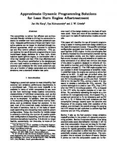
Figure 1. Summary of the proposed algorithm for finding good trajectories under a non-additive utility function.

3) Use the best rescored trajectory to construct a dataset of hstate, actioni pairs; carry out steps 1–3 until the dataset is large enough. 4) Using the dataset from steps 1–3, train a supervised learning algorithm to output the action label given the input state. As is common practice in reinforcement learning [3], this algorithm estimates the expectation in eq. (1) with a sample average over a large number of trajectories. Furthermore, as we shall see below, for our portfolio management applications, we can dispense with a generative model of trajectories by using historical data. B. Generating Good Trajectories It remains the question of generating good trajectories in the first place. This is where a K best paths algorithm is involved: under an “easier” (i.e. additive) utility function acting as a proxy for our target utility, and over a large historical time period (which will become the training set), we use the K best paths algorithm to generate the candidate trajectories of step (1) above. Obviously, both the “easier” and desired utility functions, henceforth respectively called the source and target utilities, must be correlated, so that searching for good solutions under one function has a high likelihood of yielding good solutions under the other. We discuss this point more fully below. Figure 1 illustrates schematically the complete algorithm. C. Known Uses This algorithm is certainly not the first one to make use of a K best paths algorithm: they have been used extensively in speech recognition and natural language processing (e.g. [17]). However, in these contexts, the rescored action labels found by the K best paths are either discarded (speech) or not used beyond proposing alternative hypotheses (NLP). In particular, no use is made of the rescored trajectories for training a controller. Recent publications in the reinforcement learning literature have explored the idea of converting a

14

JOURNAL OF COMPUTERS, VOL. 2, NO. 1, FEBRUARY 2007 3

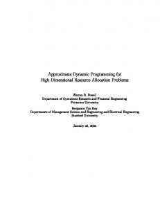
Figure 2. Intuition behind the recursive relationship underlying the REA K-best-paths algorithm; see text for details.

RL problem into a supervised learning problem [18]. However, all of the proposed approaches so far have focused on staying within an additive utility function framework and assume the presence of a generative model to construct trajectory histories. III. Enumerating the K Best Paths We rely on a very time- and memory-efficient implementation of the Recursive Enumeration Algorithm (REA) of Jim´enez and Marzal [19]. This algorithm can be made very effective by implicitly constructing a path from its differences with a previous path. It builds upon a generalization of Bellman’s recursion of eq.(3) to a statement of optimality of higher-order paths in terms of lower-order ones. Although the precise algorithm statement is not repeated for space reasons, an intuition into the algorithm’s working can be obtained from Figure 2: • Suppose that the best path to a vertex xt ends with · · · − Z − Y − xt . • According to the REA recursion, the second best path up to xt is given by the best of: 1) Either the first best path up to the immediate predecessors of xt , namely the candidate vertices {C1 , C2 , C3 }, followed by a transition to xt . 2) Or the second best path up to Y , followed by the transition b to xt . The second best path to Y is found by applying the algorithm recursively. IV. Application: Portfolio Optimization The portfolio optimization setting that we consider is a multi-period, multi-asset problem with transaction costs. We assume that the assets (e.g. stocks, futures) are sufficiently liquid that market impacts can be neglected. We invest in a universe of M asset, and the state xt at time t is given by xt = (nt,1 , . . . , nt,M , pt,1 , . . . , pt,M ) , © 2007 ACADEMY PUBLISHER

where nt,i ∈ Z is the number of shares of asset i held, and pt,i ∈ R+ is the price of asset i at time t. We can only hold an integral number of shares and short (negative) positions are allowed. The possible actions are ut ∈ ZM which are interpreted as buying or selling the number ut,i of shares asset i. To limit the search space, both nt,i and ut,i may be restricted to a small integer. The cost function gt (xt , ut ) at time t is the $ amount required to carry out ut (i.e. establish the desired position), accounting for transaction costs. As a simple example, we can take a source utility function U over all time steps as the sum of negative individual costs,1 T −1 X U (g0 , . . . , gT −1 ) = − gt . t=0

Moreover, we impose the constraints that both the initial and final portfolios be empty (i.e. they cannot hold any shares of any asset). With those constraints in place, maximizing U over a time horizon t = 0, . . . , T is equivalent to finding a strategy that maximizes the terminal wealth of the investor over the horizon. We call this source utility function the “terminal wealth” utility. Note that with this utility function, we never need to explicitly represent the cash amount on hand (i.e. it is not part of the state variables) since we use the value function itself (viz. Jt∗ (xt ) in eq. (3)) to stand for the cash currently on hand. This formulation has the advantage that we never need to discretize the cash currently being held, which allows minute price variations and small transaction costs (both fixed and proportional) to be handled without loss of precision. Other source utility functions can obviously be considered, as long as they allow a solution by dynamic programming. A notable case is the log utility (applied to the relative returns net of transaction costs) which incorporates a measure of risk aversion. In section IVC we examine an approximation to the Sharpe Ratio that yields good practical performance. A. Target Utilities Denote by υt = n0t pt the portfolio value at time t, and by υt − υt−1 ρt = υt−1 the portfolio relative return between time-steps t − 1 and t. In the experiments below, we consider two target utility functions: 1) Average Return Per Time-Step: ρ¯T =

T 1X ρt . T t=1

1 This function would incorporate a discounting factor if the horizon was very long; we assume that this is not the case.

JOURNAL OF COMPUTERS, VOL. 2, NO. 1, FEBRUARY 2007

15 4

v α u

Figure 3. Exploiting the correlation between source and target utilities: the number K of extracted paths should be large enough to adequately sample the “good target utility” region (shaded).

the quicker we should expect to find good rescored trajectories. Unfortunately, assuming the Sharpe Ratio target utility, the “maximum terminal wealth” source utility outlined above is not perfect. Although a small-but-significant positive correlation between the two is observed in practice, the lack of explicit risk aversion2 in the source utility causes some “impedance mismatch” during the search. Inspired by Moody and Saffel’s differential Sharpe Ratio [15], we attempt to define a source utility function that would be more correlated with a Sharpe Ratio (assuming this is the desired target). We define the incremental Sharpe Ratio as: ISRt =

2) Sharpe Ratio: ρ¯T − rf SRT = , σ ˆT where rf is an average government risk-free rate over the horizon, and σ ˆT is the sample standard deviation of returns σ ˆT =

1 T −1

T X

(ρt − ρ¯T )2 .

t=1

The Sharpe Ratio is one of the most widelyused risk-corrected performance measures used by portfolio managers. B. Choosing a Good K It remains to answer the question of choosing an appropriate value of K for a particular problem. Assume that, given a random trajectory i, a source utility function U and a target utility function V , the utility values of the trajectory follow a joint probability distribution p(u, v), where u = U (i) and v = V (i). This is illustrated in Figure 3. Assume further that we are interested in sampling trajectories that have at least an unconditional target utility of α or better, namely v ≥ α. Given an observed value of the source utility u, the probability that the target utility be greater than this level is given by Z ∞ 1 p(u, v˜) d˜ v, P (v ≥ α|u) = η(u) α R∞ where η(u) = −∞ p(u, v˜) d˜ v is a normalization factor. For each trajectory i, call this probability pα i . For K trajectories, the probability that at least one exceeds α under V can be approximated analytically (assuming independent draws). Hence, assuming an estimator of the joint distribution p(u, v), we can compute the number K that would yield a desired confidence of exceeding the target utility threshold α. C. Incremental Sharpe Ratio Source Utility The previous analysis suggests that the higher the correlation between the source and target utilities, © 2007 ACADEMY PUBLISHER

ρ˜t σ ˜t

where ρ˜t and σ ˜t are, respectively, exponentiallyweighted moving average (ewma) estimators of the return and volatility, using α as the ewma decay factor:3 ρ˜t

= α˜ ρt−1 + (1 − α)ρt ,

σ ˜t2

2 + (1 − α)ρ2t . = α˜ σt−1

These estimators are kept for each state and are updated using portfolio returns ρt (net of transaction costs) that are encountered along the trajectory. At first sight, it appears that keeping such running ρ˜t and σ ˜t2 estimators in the search would increase the state space size by two dimensions. However, a trick can be applied wherein those estimators are kept as the (compound) value of the state, rather than be added to the state space. In other words, when considering the Bellman equations of eqq. (2) and (3), we compute the “effective value” Jt (xt ) of a state xt as Jt (xt ) =

ρ˜t (xt ) . σ ˜t (xt )

(4)

During the K-best search, we simply update the pair ˜t2 (xt )i as though it was a single value in the h˜ ρt (xt ), σ update equation (3). This allows to perform an approximate search according to a Sharpe-like criterion at no additional cost in terms of state space size. One could legitimately wonder whether this procedure has any justification. Indeed, using eq. (4) to define the value of a state yields a non-additive cost structure. In other words, the “optimal” trajectory implied by eqq. (2) and (3) is no longer guaranteed to be the best one. Nevertheless, one could still try to apply a K-best search on the resulting graph, and observe the results. Due to the non-additivity of the incremental Sharpe Ratio criterion, the K extracted paths will not exhibit a monotonic decrease in utility (as would be normal under an additive criterion); rather, the extracted path utilities will be “noisy”, but 2 Apart from maximum position size and maximum allowed position change at each time-step. 3 In our experiments, we used α = 0.94 as the decay factor, which is the RiskMetrics-recommended standard value for daily data [20].

16

JOURNAL OF COMPUTERS, VOL. 2, NO. 1, FEBRUARY 2007 5

Figure 4. Utility as a function of the extracted path index, in the order found by the K-best-paths algorithm (K = 1 × 106 ). (Top) The source utility function (incremental Sharpe Ratio), and a smoothed version thereof (dashed line); the average source utility decreases slowly as a function of the path index. (Middle) First target utility: average return per time-step (running maximum value). (Bottom) Second target utility: Sharpe Ratio (running maximum value).

we should expect a decrease in the mean path utility as a function of the extracted path index. To illustrate the “noisy” nature of incremental Sharpe Ratio criterion, Figure 4 shows various utility functions as a function of the index of the K-th best path, when extracting 1.0×106 paths from a historical price sample.4 First, we observe that despite the noisy nature of the source utility as a function of the path index, the mean source utility decreases, as indicated by the dashed line on the top panel (resulting from a kernel-smoothing estimator the utility). Second, we note that fairly quickly, the quality of the rescored trajectories stops increasing for both the average return per time-step and Sharpe Ratio target utilities. This indicates that the source utility function captures well the traits that are required of a successful trajectory under the target utilities. Figure 5 illustrates this idea. It shows a kernel density estimate [21] of the joint distribution between U (terminal wealth utility) and V (Sharpe Ratio utility), along with the regression line between the two (dashed blue line), for the same sample path history as reported in Figure 4. We can also compute 4 Four-asset problem (futures on British Pound, Sugar, Silver, Heating Oil), allow from −3 to +3 shares of each asset in the portfolio; maximum variation of +1 or −1 share per time-step; proportional transaction costs of 0.5%, trajectory length = 30 time-steps).

© 2007 ACADEMY PUBLISHER

Figure 5. Kernel density estimate of the relationship between the incremental Sharpe Ratio (source utility) and the Sharpe Ratio (target utility) for a typical trajectory; the yellow dashed regression line underscores the strong relationship between the source and target utilities.

the relative merits of the Terminal Wealth versus Incremental Sharpe Ratio source utilities, in terms of their correlation with Average Return per timestep and Sharpe Ratio target utilities. Using again the same sample trajectory as previously, we obtain the following correlation structure between the source and target utilities:

JOURNAL OF COMPUTERS, VOL. 2, NO. 1, FEBRUARY 2007

17 6

Source Utility Terminal Wealth

Incr. Sharpe Ratio

Avg. Return

0.25

−0.20

Sharpe Ratio

0.01

0.45

V. Experimental Results We conclude by presenting results on a real-world portfolio management problem. We consider a fourasset problem on commodity futures (feeder cattle, cotton, corn, silver). Since individual commodity futures contracts expire at specific dates, we construct, for each commodity, a continuous return series by considering the return series of the contract closest to expiry, and rolling over to the next contract at the beginning of the contract expiration month. This return series is converted back into a price series. Instead of a single train–test split, the simulation is run in the context of sequential validation [22]. In essence, this procedure uses data up to t to train, then tests on the single point t + 1 (and produces a single out-of-sample performance result), then adds t + 1 to the training set, tests on t + 2, and so forth, until the end of the data. An initial training set of 1008 points (four years of daily trading data) was used. From a methodology standpoint, we proceeded in two steps: (i) computing a controller training set with the targets being the “optimal” action under the Sharpe Ratio utility, (ii) running a simulation of a controller trained with that training set, and comparing against a naive controller. We describe each in turn. A. Constructing the Training Set The construction of the training set follows the outline set forth in Figure 1 (left part). To run the K-best-paths algorithm, we allow from −1 to +1 shares of each asset in portfolio, maximum variation in each asset of −1 to +1 shares per time-step, and proportional transaction costs of 0.5%. We use, as targets in the training set, the “optimal” action under the Sharpe Ratio utility function, obtained after rescoring on 1.06 paths. Since extracting trajectories spanning several thousands time-steps is rather memory intensive, we reverted to a slightly suboptimal local-trajectory solution: • We split the initial asset price history (spanning approximately 1500 days) into overlapping 30day windows. The overlap between consecutive windows is 22 days. • We solve the Sharpe Ratio (target utility) optimization problem independently within each 30day window.5 5 In these financial experiments, we used the maximum terminal wealth source utility to construct the training set.

© 2007 ACADEMY PUBLISHER

To account for boundary effects, we drop the seven first and last actions within each window. • We concatenate the remaining actions across windows. We thus obtain the sequence of target actions across a long horizon.6 For the input part of the training set, we used: • the current portfolio state (4 elements); • the asset historical returns at horizons of length h ∈ {1, 22, 252, 378} days (16 elements). •

B. Controller Architecture Given the relatively small size of the training set, we could afford to use kernel ridge regression (KRR) as the controller architecture [23]. Any (preferably nonlinear) regression algorithm could be brought to bear. For an input vector x, the forecast given by the KRR estimator has a particularly simple form, f (x) = k(x, xi )(M + λ I)−1 y where k(x, xi ) is the vector of kernel evaluations of the test vector x against all elements of the training set xi , M is the Gram matrix on the training set, and y is the matrix of targets (in this case, the optimal actions under the Sharpe Ratio utility, found in the previous section). We made use of a standard Gaussian kernel, with σ = 3.0 and fixed λ = 10.0 (both found by crossvalidation on a non-overlapping time period). C. Results For validation purposes, we compared against two benchmarks models: • The same KRR controller architecture, but with the targets replaced by the 10-day ahead 22-day asset returns, followed by a sign(·) operation. Hence, this controller is trained to take a long position if the asset experiences a positive return over the short-term future, and symmetrically is trained to take a short position for negative returns. For this controller, the current portfolio state is not included within the inputs, since it cannot be established at training time, yielding a total of 16 inputs instead of 20. • The same targets as previously, but with a linear forecasting model (estimated by ordinary least squares) instead of KRR. Performance results over the out-of-sample period 2003–2004 (inclusive) appear in Figure 6. Further performance statistics appear in Table I. We observe that, at constant annual volatility (around 10%), the KRR model trained with the proposed methodology (Sharpe Ratio utility function) outperforms the two benchmarks. 6 It is obvious that this approach will not capture long-range dependencies between actions (more than 30 days in this case). However, for the specific case of the Sharpe Ratio, the impact of an action is not usually felt at a long distance, and thus this approach was found to work well in practice. Needless to say, it will have to be adjusted to other more complex utility functions.

18

JOURNAL OF COMPUTERS, VOL. 2, NO. 1, FEBRUARY 2007 7

Linear return predictor (long-short positions) / Ann.IR = -0.315 Kernel ridge regression return predictor (long-short positions) / Ann.IR = 0.113 Kernel ridge regression ''optimal decisions'' / Ann.IR = 0.369

Cumulative Return

10%

5%

0%

-5%

2003

2004 Date

2005

Figure 6. Out-of-sample financial simulation results for the 2003–2004 period, comparing a controller trained with the proposed algorithm (solid red; Information Ratio = 0.369) against two benchmark models (resp. IR=−0.315 for linear controller (dotted blue) and IR=0.113 for KRR controller (dashed green)). TABLE I. Financial performance statistics for the out-of-sample simulation results on the 2003–2004 period.

Avg monthly relative return Monthly return std dev. Worst monthly return Best monthly return Annual Information Ratio† Avg daily net exposure Avg effective leverage Avg monthly turnover Avg daily hit ratio †

Benchmark Linear −0.14% 2.68% −5.80% 5.15% −0.31 −5.3% 74.7% 499% 48.1%

Benchmark KRR 0.20% 2.89% −6.21% 6.80% 0.11 10.8% 73.4% 175% 50.6%

Sharpe Ratio “Optimal” Targets/KRR 0.43% 3.07% −7.14% 6.73% 0.37 28.3% 59.6% 80% 51.6%

with respect to U.S. 3-month T-Bill.

VI. Discussion and Future Work The current results, although demonstrating the value of the proposed algorithm, raise more questions than they answer. In particular, we did not consider the impact on rescoring performance of the choice of source utility function. Moreover, we so far ignored the major efficiency gains that can be achieved by an intelligent pruning of the search graph, either in the form of beam searching or action enumeration heuristics. Another question that future work should investigate is that with the methodology proposed here, the supervised learning algorithm optimizes the controller with respect to a regression (or classification) criterion which can disagree with the target utility when the target training set trajectory is not perfectly reproduced. In order to achieve good generalization, because of unpredictability in the data and because of the finite sample size, the trained controller will most likely not reach the supervised learning targets corresponding to the selected trajectory. However, among all the controllers that do not reach these targets and that are reachable by the learning algo© 2007 ACADEMY PUBLISHER

rithm, we will choose one that minimizes an ordinary regression or classification criterion, rather than one that maximizes our financial utility. Ideally, we would like to find a compromise between finding a “simple” controller (from a low-capacity class) and finding a controller which yields high empirical utility. One possible way to achieve such a trade-off in our context would be to consider the use of a weighted training criterion (e.g. similar to ones used to train boosted weak learners in Adaboost [24]) that penalizes regression or classification errors more or less according to how much the target utility would decrease by taking the corresponding “wrong” decisions, different from the target decision.

References [1] R. Bellman, Dynamic Programming. NJ: Princeton University Press, 1957. [2] D. P. Bertsekas, Dynamic Programming and Optimal Control, 2nd ed. Belmont, MA: Athena Scientific, 2001, vol. I. [3] D. P. Bertsekas and J. N. Tsitsiklis, Neuro-Dynamic Programming. Belmont, MA: Athena Scientific, 1996. [4] R. S. Sutton and A. G. Barto, Reinforcement Learning: An Introduction. Cambridge, MA: MIT Press, 1998. [5] J. Si, A. G. Barto, W. B. Powell, and D. Wunsch, Eds., Handbook of Learning and Approximate Dynamic Programming, ser. IEEE Press Series on Computational Intelligence) (Hardcover. Wiley–IEEE Press, 2004. [6] J. Mossin, “Optimal multiperiod portfolio policies,” The Journal of Business, vol. 41, no. 2, pp. 215–229, 1968. [7] P. A. Samuelson, “Lifetime portfolio selection by dynamic stochastic programming,” The Review of Economics and Statistics, vol. 51, no. 3, pp. 239–246, 1969. [8] R. C. Merton, “Lifetime portfolio selection under uncertainty: The continuous-time case,” The Review of Economics and Statistics, vol. 51, no. 3, pp. 247– 257, 1969. [9] W. F. Sharpe, “Mutual fund performance,” Journal of Business, pp. 119–138, January 1966. [10] ——, “The sharpe ratio,” The Journal of Portfolio Management, vol. 21, no. 1, pp. 49–58, 1994. [11] R. C. Grinold and R. N. Kahn, Active Portfolio Management. McGraw Hill, 2000. [12] F. Sortino and L. Price, “Performance measurement in a downside risk framework,” The Journal of Investing, pp. 59–65, Fall 1994. [13] D. P. Bertsekas, Nonlinear Programming, 2nd ed. Belmont, MA: Athena Scientific, 2000. [14] Y. Bengio, “Using a financial training criterion rather than a prediction criterion,” International Journal of Neural Systems, vol. 8, no. 4, pp. 433–443, 1997. [15] J. Moody and M. Saffel, “Learning to trade via direct reinforcement,” IEEE Transactions on Neural Networks, vol. 12, no. 4, pp. 875–889, 2001. [16] N. Chapados and Y. Bengio, “Cost functions and model combination for VaR-based asset allocation using neural networks,” IEEE Transactions on Neural Networks, vol. 12, pp. 890–906, Juillet 2001. [17] L. Rabiner and B. Juang, Fundamentals of Speech Recognition. Prentice Hall, 1993.

JOURNAL OF COMPUTERS, VOL. 2, NO. 1, FEBRUARY 2007

19 8

[18] J. Langford and B. Zadrozny, “Relating reinforcement learning performance to classification performance,” in 22nd International Conference on Machine Learning (ICML 2005), Bonn, Germany, August 2005. [19] V. M. Jim´enez Pelayo and A. Marzal Var´ o, “Computing the K shortest paths: a new algorithm and an experimental comparison,” in Proc. 3rd Worksh. Algorithm Engineering, July 1999. [Online]. Available: http://terra.act.uji.es/REA/papers/wae99.ps.gz [20] RiskMetrics, “Riskmetrics—technical document,” J.P. Morgan, New York, NY, Tech. Rep., 1996, http://www.riskmetrics.com. [21] M. Wand and M. Jones, Kernel Smoothing. London: Chapman and Hall, 1995. [22] Y. Bengio and N. Chapados, “Extensions to metric based model selection,” Journal of Machine Learning Research, vol. 3, no. 7–8, pp. 1209–1228, October– November 2003. [23] J. Shawe-Taylor and N. Cristianini, Kernel Methods for Pattern Analysis. Cambridge University Press, 2004. [24] Y. Freund and R. E. Schapire, “Experiments with a new boosting algorithm,” in Machine Learning: Proceedings of Thirteenth International Conference, 1996, pp. 148–156.

© 2007 ACADEMY PUBLISHER