Mar 5, 2001 - as any that I have submitted or am currently submitting for a degree, diploma or any other ...... The design of the calculi involves a delicate trade-off â many ...... implies there exists LP1,...,LPn such that, letting LP = LP0 and LQ = LPn+1, we have ...... (POPL) (St. Petersburg Beach, Florida), January 1996.
Nomadic π-Calculi: Expressing and Verifying Communication Infrastructure for Mobile Computation
Asis Unyapoth Pembroke College University of Cambridge
This dissertation is submitted for the degree of Doctor of Philosophy 5 March 2001
Abstract This thesis addresses the problem of verifying distributed infrastructure for mobile computation. In particular, we study language primitives for communication between mobile agents. They can be classified into two groups. At a low level there are location dependent primitives that require a programmer to know the current site of a mobile agent in order to communicate with it. At a high level there are location independent primitives that allow communication with a mobile agent irrespective of any migrations. Implementation of the high level requires delicate distributed infrastructure algorithms. In earlier work of Sewell, Wojciechowski and Pierce, the two levels were made precise as process calculi, allowing such algorithms to be expressed as encodings of the high level into the low level; a distributed programming language Nomadic Pict has been built for experimenting with such encodings. This thesis turns to semantics, giving a definition of the core language (with a type system) and proving correctness of an example infrastructure. This involves extending the standard semantics and proof techniques of process calculi to deal with the new notions of sites and agents. The techniques adopted include labelled transition semantics, operational equivalences and preorders (eg. expansion and coupled simulation), “up to” equivalences, and uniform receptiveness. We also develop two novel proof techniques for capturing the design intuitions regarding mobile agents: we consider translocating versions of operational equivalences that take migration into account, allowing compositional reasoning; and temporary immobility, which captures the intuition that while an agent is waiting for a lock somewhere in the system, it will not migrate. The correctness proof of an example infrastructure is non-trivial. It involves analysing the possible reachable states of the encoding applied to an arbitrary high-level source program. We introduce an intermediate language for factoring out as many ‘house-keeping’ reduction steps as possible, and focusing on the partially-committed steps.
iii
iv
Declaration Except where otherwise stated in the text, this thesis is the result of my own work and is not the outcome of work done in collaboration. This dissertation is not substantially the same as any that I have submitted or am currently submitting for a degree, diploma or any other qualification at any other university. No part of this dissertation has already been or is being concurrently submitted for any such degree, diploma or any other qualification. This dissertation does not exceed sixty thousand words, including tables, footnotes and bibliography.
v
Acknowledgements I would like to express my gratitude to my supervisor, Peter Sewell, who gave me directions in this research and helpful suggestions when I encountered hard problems. I thank him most of all for having been patient with my ignorance of the subject, as well as of the English grammar. Prof. Robin Milner has been a great inspiration for this thesis. I attended his lectures on communicating automata and the π-calculus, and was immediately fascinated by this new way of looking at computation. This led me to an engagement in a project of implementing a concurrent application using the programming language Pict. In this project, I also had the opportunity of working with a co-author of Pict, Benjamin Pierce, as well as Peter Sewell. During this time, I learned a great deal about many research areas in the field of theoretical computer science, especially those involving process calculi and types. It was then that my interest in applying the π-calculus to real distributed systems began. I wish to thank Pawel Wojciechowski, who took part in the design and implementation of Nomadic π-calculi, for many discussions on distributed algorithms and mobile computation. I also thank Lucian Wischik for proof-reading and for his comments. During the time of this research, I regularly attended the meetings of the Opera Group, and, thanks to such meetings, I was able to keep in touch with the real world. Seminars organised by the Computer Laboratory, the Theory and Semantics Group also gave me chances to learn about much interesting ongoing research. This research (and my education in England prior to that) was supported by the Royal Thai Government Students’ Scholarship. I am greatly in debt of this many years of continuous and generous support, without which I would have no chance of studying in England. More personally, I would like to thank my family in Thailand for tolerating my long absence, and my friends in Cambridge for keeping me sane. Thanks also to my house-mates for looking vii
viii after my well-being (not to mention tolerating my eccentric behaviour) during the final period of my research.
Contents Main Notations
xv
1 Introduction
1
1.1
An Overview of Mobile Computation . . . . . . . . . . . . . . . . . . . . . . .
3
1.2
Infrastructures and Location-Independence . . . . . . . . . . . . . . . . . . .
4
1.3
Verifying Infrastructures . . . . . . . . . . . . . . . . . . . . . . . . . . . . . .
6
1.4
Nomadic π-Calculi . . . . . . . . . . . . . . . . . . . . . . . . . . . . . . . . .
7
1.5
Thesis Contribution . . . . . . . . . . . . . . . . . . . . . . . . . . . . . . . .
8
1.6
Outline . . . . . . . . . . . . . . . . . . . . . . . . . . . . . . . . . . . . . . .
9
2 Background 2.1
2.2
2.3
11
Asynchronous π-Calculus . . . . . . . . . . . . . . . . . . . . . . . . . . . . .
12
2.1.1
Syntax . . . . . . . . . . . . . . . . . . . . . . . . . . . . . . . . . . . .
13
2.1.2
Operational Semantics . . . . . . . . . . . . . . . . . . . . . . . . . . .
14
Nomadic π-Calculi . . . . . . . . . . . . . . . . . . . . . . . . . . . . . . . . .
17
2.2.1
Types . . . . . . . . . . . . . . . . . . . . . . . . . . . . . . . . . . . .
18
2.2.2
Type contexts . . . . . . . . . . . . . . . . . . . . . . . . . . . . . . . .
19
2.2.3
Values, Patterns and Expressions . . . . . . . . . . . . . . . . . . . . .
20
2.2.4
Processes . . . . . . . . . . . . . . . . . . . . . . . . . . . . . . . . . .
22
Centralised Server Translation . . . . . . . . . . . . . . . . . . . . . . . . . . .
25
ix
x
CONTENTS
3 Type System
33
3.1
Forms of Typing Judgement . . . . . . . . . . . . . . . . . . . . . . . . . . . .
33
3.2
Subtyping Rules . . . . . . . . . . . . . . . . . . . . . . . . . . . . . . . . . .
34
3.3
Type and Type Context Formation . . . . . . . . . . . . . . . . . . . . . . . .
35
3.4
Values and Expressions . . . . . . . . . . . . . . . . . . . . . . . . . . . . . .
37
3.5
Patterns . . . . . . . . . . . . . . . . . . . . . . . . . . . . . . . . . . . . . . .
38
3.6
Basic and Located Process . . . . . . . . . . . . . . . . . . . . . . . . . . . . .
39
3.7
Basic Properties . . . . . . . . . . . . . . . . . . . . . . . . . . . . . . . . . .
41
3.8
Type-Preserving Substitution and Matching . . . . . . . . . . . . . . . . . . .
42
4 Operational Semantics
45
4.1
Structural Congruence . . . . . . . . . . . . . . . . . . . . . . . . . . . . . . .
46
4.2
Reduction Semantics . . . . . . . . . . . . . . . . . . . . . . . . . . . . . . . .
48
4.3
Labelled Transition Semantics . . . . . . . . . . . . . . . . . . . . . . . . . . .
51
4.4
Runtime Errors . . . . . . . . . . . . . . . . . . . . . . . . . . . . . . . . . . .
59
4.5
Properties of the Semantics . . . . . . . . . . . . . . . . . . . . . . . . . . . .
61
5 Operational Equivalences
65
5.1
Background . . . . . . . . . . . . . . . . . . . . . . . . . . . . . . . . . . . . .
66
5.2
Bisimulations . . . . . . . . . . . . . . . . . . . . . . . . . . . . . . . . . . . .
69
5.3
Translocating Equivalences . . . . . . . . . . . . . . . . . . . . . . . . . . . .
71
5.3.1
Basic Properties . . . . . . . . . . . . . . . . . . . . . . . . . . . . . .
74
5.3.2
Congruence Properties . . . . . . . . . . . . . . . . . . . . . . . . . . .
76
Other Operational Relations . . . . . . . . . . . . . . . . . . . . . . . . . . . .
80
5.4.1
Expansions . . . . . . . . . . . . . . . . . . . . . . . . . . . . . . . . .
80
5.4.2
Coupled Simulations . . . . . . . . . . . . . . . . . . . . . . . . . . . .
82
5.4
CONTENTS
xi
6 Proof Techniques
87
6.1
Techniques of Bisimulation “Up To” . . . . . . . . . . . . . . . . . . . . . . .
87
6.2
Channel-Usage Disciplines . . . . . . . . . . . . . . . . . . . . . . . . . . . . .
89
6.2.1
Non-sendability . . . . . . . . . . . . . . . . . . . . . . . . . . . . . . .
90
6.2.2
Access Restrictions . . . . . . . . . . . . . . . . . . . . . . . . . . . . .
91
6.2.3
Uniform Receptiveness . . . . . . . . . . . . . . . . . . . . . . . . . . .
95
6.2.4
Local Channels . . . . . . . . . . . . . . . . . . . . . . . . . . . . . . .
98
6.3
Determinacy and Confluence . . . . . . . . . . . . . . . . . . . . . . . . . . . 100
6.4
Temporary Immobility . . . . . . . . . . . . . . . . . . . . . . . . . . . . . . . 104
6.5
Maps and Their Operators . . . . . . . . . . . . . . . . . . . . . . . . . . . . . 110
7 The Correctness Proof
117
7.1
Background . . . . . . . . . . . . . . . . . . . . . . . . . . . . . . . . . . . . . 119
7.2
The Intermediate Language . . . . . . . . . . . . . . . . . . . . . . . . . . . . 121
7.3
7.4
7.2.1
Type System . . . . . . . . . . . . . . . . . . . . . . . . . . . . . . . . 127
7.2.2
Labelled Transition Rules . . . . . . . . . . . . . . . . . . . . . . . . . 130
Factorisation of C-Encoding . . . . . . . . . . . . . . . . . . . . . . . . . . . . 135 7.3.1
Loading . . . . . . . . . . . . . . . . . . . . . . . . . . . . . . . . . . . 136
7.3.2
Flattening . . . . . . . . . . . . . . . . . . . . . . . . . . . . . . . . . . 137
7.3.3
Behavioural Properties . . . . . . . . . . . . . . . . . . . . . . . . . . . 139
Decoding Systems into Source Programs . . . . . . . . . . . . . . . . . . . . . 144 7.4.1
7.5
Behavioural Properties . . . . . . . . . . . . . . . . . . . . . . . . . . . 146
The Main Result . . . . . . . . . . . . . . . . . . . . . . . . . . . . . . . . . . 149
8 Related Models 8.1
Process calculi-based models 8.1.1
151 . . . . . . . . . . . . . . . . . . . . . . . . . . . 153
Verification and Proof Techniques . . . . . . . . . . . . . . . . . . . . 160
xii
CONTENTS 8.1.2
Programming Languages . . . . . . . . . . . . . . . . . . . . . . . . . . 163
8.1.3
Discussion . . . . . . . . . . . . . . . . . . . . . . . . . . . . . . . . . . 164
8.2
I/O Automata . . . . . . . . . . . . . . . . . . . . . . . . . . . . . . . . . . . 167
8.3
Mobile UNITY . . . . . . . . . . . . . . . . . . . . . . . . . . . . . . . . . . . 171
9 Conclusions and Future Work
175
9.1
Summary . . . . . . . . . . . . . . . . . . . . . . . . . . . . . . . . . . . . . . 175
9.2
Future Work . . . . . . . . . . . . . . . . . . . . . . . . . . . . . . . . . . . . 176
9.3
Conclusion . . . . . . . . . . . . . . . . . . . . . . . . . . . . . . . . . . . . . 181
A A Forwarding-Pointers Infrastructure Translation
183
A.1 Sketch of Intermediate Language . . . . . . . . . . . . . . . . . . . . . . . . . 186
B Meta-Theoretic Results
189
B.1 Structural Congruence and the Type System . . . . . . . . . . . . . . . . . . 189 B.2 Operational Semantics . . . . . . . . . . . . . . . . . . . . . . . . . . . . . . . 192 B.3 Subject Reduction . . . . . . . . . . . . . . . . . . . . . . . . . . . . . . . . . 203 B.4 (Cong-L) Absorption . . . . . . . . . . . . . . . . . . . . . . . . . . . . . . . 206 B.5 Semantics Matching . . . . . . . . . . . . . . . . . . . . . . . . . . . . . . . . 208 B.6 Translocating Relations . . . . . . . . . . . . . . . . . . . . . . . . . . . . . . 211 B.7 Congruence Result . . . . . . . . . . . . . . . . . . . . . . . . . . . . . . . . . 215 B.8 Proof Techniques . . . . . . . . . . . . . . . . . . . . . . . . . . . . . . . . . . 221 B.9 ∆-Restricted Equivalences . . . . . . . . . . . . . . . . . . . . . . . . . . . . . 224
C Properties of Temporary Immobility
227
C.1 Proofs of C-Related Results . . . . . . . . . . . . . . . . . . . . . . . . . . . . 232
CONTENTS D Correctness Proof
xiii 245
D.1 General Properties . . . . . . . . . . . . . . . . . . . . . . . . . . . . . . . . . 245 D.2 Analysis of F [[·]] . . . . . . . . . . . . . . . . . . . . . . . . . . . . . . . . . . 249 D.3 Analysis of D [[·]] . . . . . . . . . . . . . . . . . . . . . . . . . . . . . . . . . . 265 Technical Terms . . . . . . . . . . . . . . . . . . . . . . . . . . . . . . . . . . . . . 297 Bibliography
275
Technical Terms
297
Main Notations Below are the main notations used in this thesis. The page numbers refer to the page in which the notation is defined.
Functions f :A→B
f is a partial function from A to B
f ⊕ a 7→ b
the function like f except that a is mapped to b
f, a 7→ b
the function like f with a 6∈ dom(f ) is mapped to b
f +g
the sum of functions f and g with dom(f )∩dom(g) = ∅
Sets F
basic functions
21
T
base types
18
TV
type variables
18
X
names
13
nπLD,LI
high-level located processes
24
nπLD
low-level located processes
24
IL
systems in the intermediate language
117
Structural Congruences Γ≡Ξ LP ≡ LQ
20 46
P ≡Q Sys ≡Φ xv
46 Sys0
130
Well-Formedness and Typing Judgements `Γ
for unlocated type contexts
35
`L Γ
for located type contexts
35
` Φ ok
for valid system contexts
129
Γ`T
for type
35
Γ ` x@s
for locating names
38
Γ`e∈T
for values and expressions
37
Γ ` ls ∈ List T
for lists
111
Γ`p∈T .∆
for patterns
38
Γ `a P
for basic process
39
Γ ` LP
for located process
39
Φ ` Sys ok
for systems in the intermediate language
128
Operational Semantics and Relations Γ LP
configuration
48
reduction relation
48
Γ a P − → LP
labelled transition (basic processes)
52
Γ LP − → LQ
labelled transition (located processes)
53
∼ ˙Γ
strong bisimulation
70
∼ ˙M Γ
translocating strong bisimulation
74
∼Γ
strong congruence
78
˙Γ ≈ ˙M ≈ Γ
weak bisimulation
70
translocating weak bisimulation
74
≈Γ
weak congruence
78
˙M � Γ
translocating expansion
81
�Γ
expansion congruence
81
�Γ
coupled simulation
84
Γ LP − →
Γ0
LQ
α
∆ β
∆
Auxiliary Definitions for the C-Translation Φaux
27
Φ− aux
108
ΩD
106
Ωaux
106
xvi
Miscellaneous det
Γ LP −−→ LQ
deterministic reduction
101
eval(ev)
evaluations
21
match(p, v)
matching
43
fv(P )
free variables of P
25
fv(LP )
free variables of LP
25
mayMove(LP )
potentially migrating agents in LP
76
agents(LP )
agents in LP
99
readA(c, LP )
agents which use c for input in LP
99
writeA(c, LP )
agents which use c for output in LP
99
fv(T )
free variables in T
19
fv(Γ)
free variables in Γ
20
dom(Γ)
domain of Γ
20
range(Γ)
range of Γ
20
agents(Γ)
agents declared in Γ
72
mov(Γ)
mobile agents declared in Γ
72
M1 ]β M2
‘translocating union’
73
Γ ⊕ a 7→ s
updating Γ with a at site s
50
Γβ
updating Γ with β
69
M
xvii
Chapter 1
Introduction The explosive increase of the Internet’s popularity has quickly been exploited by users, programmers and business alike, as evident from the rapid growth of Internet applications and electronic commerce. The development of network applications are often hindered, however, by many problems particular to large area networks: those of efficiency, reliability, and security. Mobile computations, in which agents may move between machines, are considered by many to be a promising paradigm for thinking about and structuring network applications. Chess et al. in their assessment [CHK97] argued that, while mobile agents retain no particularly strong advantages over other alternatives in implementing certain functions, they provide a generalised framework for solving many existing problems. Furthermore, mobile agents also enable new, derivative network services and hence businesses. An essential feature of mobile computation is the ability of agents to interact. This is how they access resources (on physical machines as well as on other agents) and exchange information. Existing technologies offer a variety of ways in which agents may interact — they can be classified as location dependent (LD) or location independent (LI) interactions. The former requires an agent to know the exact location of the target agent it wishes to interact with; the programmers must also ensure that the target agent does not migrate away while the message is routed to the destination. For ease of writing application using mobile agents, we need the latter form of communication which allows agents to interact without explicitly tracking each other’s movement. Location-independent communication is not supported by the standard network technology. Several programming languages which provide location independence (eg. Facile [TLK96] and the Join language [FGL+ 96]) have some distributed infrastructure algorithms hard-coded into 1
2
CHAPTER 1. INTRODUCTION
their implementations. It is problematic to apply this technology to wide-area networks for at least two reasons. First, it should be possible to provide different infrastructure algorithms for different applications, so that one may choose an algorithm with satisfactory range of performance matching the requirement of each application. Secondly, distributed algorithms are delicate and error-prone; the correctness of their behaviour is crucial, but difficult to verify without clear semantics or levels of abstraction. A wide-area programming language should therefore allow more flexibility by providing a low-level abstraction for distribution and network communication; location-independence (or other higher-level abstraction) can then be expressed in terms of the low-level abstraction, using the modularisation facilities of the language. In [SWP99], the two levels of abstraction were made precise by giving them corresponding high- and low-level Nomadic π-calculi. The calculi are extensions of the asynchronous πcalculus [MPW92] with the notions of sites and agents. Programming using these notions requires new primitives: the low-level calculus adds those for agent creation, migration of agents between sites, and location-dependent communication between agents. To these, the high-level calculus adds a primitive for location-independent communication, suitable for writing applications. A distributed infrastructure algorithm for supporting locationindependent communication can then be expressed as an encoding from the high-level calculus to the low-level calculus. The earlier work of Sewell et al. [SWP99] gave the syntax, a reduction semantics of Nomadic π-calculi, as well as two such encodings, based on centralforwarding-server and forwarding-pointer algorithms. A programming language based on the calculi, Nomadic Pict, has been implemented by Wojciechowski [WS99, Woj00a], building on the Pict implementation of Pierce and Turner [PT00]. The focus of this thesis is on developing the semantics and proof techniques for verifying distributed infrastructure algorithms. This involves extending the existing techniques of process calculi to deal with the new notions of sites and mobile agents. Mobile agents, in particular, require novel semantic techniques for capturing design intuitions, such as “while an agent is waiting for an acknowledgement from the daemon, it may not migrate.” Being able to verify distributed infrastructures gives one an assurance that agents may always communicate in the location-independent mode, even in the most complex programs involving frequently-migrating agents. It is also a step towards a semantic foundation of richer widearea distributed computing, which one may use for verifying correctness and robustness properties of programs in the presence of failure and malicious attack. This chapter introduces some of the concepts and keywords relating to mobile computations. In Section 1.1, we give a broad overview of mobility in wide-area networks. We briefly discuss
1.1. AN OVERVIEW OF MOBILE COMPUTATION
3
various means, advantages and areas of mobility (including process migration, mobile-device computing and mobile agents). Section 1.2 discusses the distributed infrastructure needed for supporting mobility and gives various existing examples. We give a few reasons why they are seen as problematic and a major challenge in employing mobility in wide-area networks. Section 1.3 discusses verification of such infrastructures: why it is necessary, why it is hard, and what support is required. We describe the Nomadic π-calculi in Section 1.4 and give reasons why they are suitable for such a task. In all these sections, we refrain from discussing in detail the related implementation issues. Readers may refer to various overviews and surveys [FPV98, MDW99, Woj00a] for further details and background. In Section 1.5, we outline the contribution this thesis made to research on the semantics and verification of programming languages with mobility. We conclude this chapter by giving the outline of the content of this thesis.
1.1
An Overview of Mobile Computation
The term “mobile computation” is used in several contexts, and can sometimes cause confusion. Miloji˘ci´c et al. in [MDW99] discussed mobility in three major areas: process migration, mobile computation and mobile agents. • Process migration is the act of transferring a process between two computers. A process here is an operating system abstraction that comprises the code, data and operating system state associated with an instance of a running application. Traditionally, process migration is used for enabling load distribution (by moving processes to lightly-loaded machines) and fault resilience (by moving processes from machines that are likely to fail). An aim of systems supporting this type of mobility is to provide transparency to the users, making processes appear as though they were running on the same machine. Systems supporting process migration can be classified as those which are integrated with the operating system and those which are running at the user level. The former includes the operating systems MOSIX [BL85, BS85], Sprite [OCD+ 87, DO91], and Charlotte [AF89]. The latter are typically less efficient, but simple to maintain and to port to new systems. These include Condor [LS92] and Emerald [JLHB88]. • Mobile computation involves the physical movement of hardware, such as laptop and palmtop computers. These devices are becoming increasingly popular; many of today’s mobile phones, for example, provide Internet access and electronic mail. Phys-
4
CHAPTER 1. INTRODUCTION ical mobility shares similarities with “logical” process mobility, but there are specific issues as well — for example, disconnected operation (an ability of devices to perform computation while disconnected to the network), and the problem of limited resources (eg. battery). Readers may refer to [FZ94] for an overview of challenges in this area. This type of mobility is beyond the scope of this thesis. We shall use the terms device mobility when we need to refer this type of mobility. We also use the term mobile-device network for referring to network which supports device mobility. • Mobile agents are units of executing computation that can move between machines in the network, autonomously executing tasks on behalf of users. Here Miloji˘ci´c et al. distinguished mobile agents from mobile code (such as Java applets) by the fact that mobile agents also carry data and possibly threads of control, allowing the execution of an agent to be suspended and resumed once it moves to another site. They are generally supported at the user level by programming languages such as Telescript [Whi95], Agent Tcl [Gra96], Aglets [LO98], Voyager [Gla98], Concordia [WPW98], Sumatra [ARS97], and JoCaml [Fes98, CF99]. Contrary to mobile agents, in the mobile code paradigm only code — and not data or threads of control — may move from one site to another. In Java [GJS97, LY97], an application can dynamically download applets from the network and execute them locally. Other languages employing this paradigm include Facile [TLP+ 93], TACOMA [JRS94], and M0 [Tsc94].
All these types of mobility offer many benefits, including ability to move towards a distributed resource (and hence reduce network overhead), ease of reconfiguration, increases in reliability, and (for mobile-device networks) support for disconnected operations. Mobile agents, in particular, are intended to be used for programming wide-range of applications, including electronic commerce, software distribution and updates, information retrieval, system administration, and network management.
1.2
Infrastructures and Location-Independence
In order to employ mobility in global networks and make use of their services, some underlying mechanism (which we shall refer to as distributed infrastructure) is required for supporting the following. • Mobility This includes support for movement of processes, agents and devices, disconnected operation, and binding to local resources. Moving an agent, for example,
1.2. INFRASTRUCTURES AND LOCATION-INDEPENDENCE
5
involves suspending its execution, encoding the agent for transmission, transmitting to the new host, decoding and resuming the execution at the new host. • Interaction In performing its tasks, an agent should be able to interact with its host, with other agents, and with the users. This is how an agent will access resources (where such resources can be on its hosts or on other agents), and exchange information. In a mobile-device network, an infrastructure should ensure that packets sent to a moving host do not get lost and hence eventually reach their target. • Heterogeneity Users of the global network are likely to access services from different machine environments. The distributed infrastructure must therefore allows agents to be executed on machines of any type of architecture. • Security This is one of the major concerns of mobile computation: how to protect agents from hostile execution environments, and how to protect execution environments from hostile agents such as viruses and worms. An infrastructure should provide some degree of protection (cf. [Nec97]). There are numerous examples of distributed infrastructures. Mobile IP [IJ93] is a set of IPbased protocols which enables mobile machines to keep their network connections while they move in a network environment. Running an application written in a mobility-supporting programming language (eg. Telescript) requires a wide-spread runtime system (the Telescript Protocol) which enables agent transport and execution on heterogeneous machine environment. Other examples are object-based RPC systems, such as CORBA [OMG96] and DCOM [EE98]; these provide transparent access to a distributed collection of objects, hiding the true locations of objects and details of how messages are routed to their destinations. Here we shall concentrate on support for interaction between agents. As discussed, these can be classified as location dependent and location independent. In the first, an agent a may interact with another agent b only if a knows the exact location of b. There are many examples of this: Telescript agents must be at the same place in order to interact (using an explicit meet operation); Agent Tcl uses an RPC-like mechanism, allowing client agents to access services of (static) server agents, whose locations can be looked up from a nameserver agent. In the second, an agent can interact with another agent without knowing its location. This allows agents to communicate without explicitly tracking movements of one another. This is supported by many languages, such as Facile [TLP+ 93], Voyager [Gla98], the Join language [FG96, FM97], MOA [MCR+ 96], and Mobile Object Workbench (MOW) [BHDH98].
6
CHAPTER 1. INTRODUCTION
Location independence, however, is not supported by standard network technologies. It requires an infrastructure for tracking the movements of agents. Facile uses node servers to forward messages on a channel to the site where such a channel is created. In Voyager, an object may send a message to another object via its ‘virtual reference’ to object; these forward messages to the actual target remote object. MOA and MOW use an explicit name server for tracking locations of agents — agents are therefore required to register with the name server and inform it whenever they move. The Join Language also uses similar mechanism, although the interaction between agents and the name server is hidden in the implementation. Sewell, Wojciechowski and Pierce [SWP99] argued that application of distributed infrastructures in wide-area networks is problematic for many reasons. First of all, distributed infrastructure are somewhat application-specific — different applications require different degrees of mobility, interactions and fault tolerance. This argument recalls that of Waldo et al. [WWWK94], who argue against a unified view of objects which reside in the same machines and objects which reside in different machines. Programmers, they argued, should be aware of latency, have a model of memory access, and take into account issues of concurrency and partial failure. The lack of such an awareness can lead to systems that are unreliable and incapable of scaling beyond small groups of machines. Similar polemic, although against network transparency for supporting fault tolerance, is given by Vogels et al. [VvRB98]. The second problem of distributed infrastructures, which is central to this thesis, is that they are delicate and error-prone, which can make them difficult to reason about. We discuss this in more detail in the next section.
1.3
Verifying Infrastructures
People hope to use mobile agents in a wide range of applications, including electronic commerce. Distributed infrastructures are necessary for mobile agents, and are therefore crucial to such applications. Subtle errors of infrastructure algorithms could be disastrous — financially or otherwise. It is therefore natural to demand some sort of assurance that programs will behave as they are expected. The formal proof of correctness is known as verification. Verifying distributed infrastructures is difficult without clear level of abstraction or semantic definition. The descriptions of algorithms employed in Mobile IP, and of the agent tracking mechanisms mentioned above, are given informally in natural language. This can be ambiguous since natural language text cannot sufficiently describes algorithms which are highly concurrent and require delicate mechanisms for ensuring absence of race conditions, deadlock
1.4. NOMADIC π-CALCULI
7
and other errors. Besides, no formal properties can be derived from such description, given the lack of formal semantics. There are many existing methods capable of verifying distributed algorithms — most prominent are perhaps the I/O automata model [LT87, LT88] and mobile UNITY [RMP97] (an overview of these and other methods is given in Chapter 8). The problem with the existing methods, as Garland and Lynch [GL98] argue, is the lack of formal connection between verified designs and the corresponding final code. It is often feasible to prove a distributed algorithm correct, whether by hand or by using some mechanised tools, such as theorem provers. The verified algorithm, however, must be translated by hand from the pseudo-code or other mathematical constructs in which it was expressed into a real distributed programming language (eg. C++ or Java) before it can be used in a real distributed systems. This process can be difficult, time-consuming and error-prone. A programming language for distributed systems should therefore be suitable for both verification and code generation. This can be problematic, for the features which make a language suitable for verification (axiomatic style, simplicity and nondeterminism) are different from those that make it suitable for code generation (operational style, expressive power and determinism).
1.4
Nomadic π-Calculi
The Nomadic π-calculi [SWP99] have been formulated out of the need for expressing distributed infrastructures in a precise manner, for experimenting with different underlying algorithms, and for reasoning about them. The calculi offer a two-level framework: the low-level consists of a set of well-understood, location-dependent primitives for programming mobile computations — agent creation, agent migration, and communication of asynchronous messages between agents; the high-level adds a location-independent primitive, allowing agents to interact irrespective of where they are, convenient for writing applications. Distributed infrastructures can be expressed precisely as translations from the high-level calculus to the low-level calculus. The operational semantics of the calculi provide a precise understanding of the algorithms’ behaviour. This supports proofs of their correctness and, ultimately, of their robustness. The calculi are suitable for verification of distributed and mobile computations for two reasons. Firstly, their theoretical basis is supported by the fact that it is based on an asynchronous π-calculus [MPW92], which offers a clear treatment of concurrency and process communication. The theoretical basis of the π-calculus has become solid over the years,
8
CHAPTER 1. INTRODUCTION
providing a variety of techniques for reasoning about process behaviour. It has been criticised for the lack of notions of locality and distribution — arguably the two most essential features in distributed systems. Nomadic π addresses this by adding the notions of sites and agents, allowing distribution and locality to be precisely described. Secondly, programs expressed in Nomadic π-calculi can be used for generating executable code, since Nomadic Pict, a programming language based on the calculi, has been implemented by Wojciechowski [WS99, Woj00a, Woj00b]. It builds on the Pict language of Pierce and Turner [PT00], a concurrent, though not distributed, language based on the asynchronous π-calculus. Pict supports fine-grain concurrency and the communication of asynchronous messages. To these, low- and high-level Nomadic Pict add location-dependent and location-independent primitives, corresponding to the two calculi. In contrast to other languages which provide location-independent primitives, Nomadic Pict allows programmers to provide their own infrastructure for an application at compile time. An arbitrary infrastructure for implementing location-independent primitives can be expressed as a user-defined translation into the low-level language, which can then be deployed dynamically at runtime. The ease of expressing infrastructure algorithms encourages programmers to experiment with wide-range of infrastructures for applications with different migration and communication patterns. The language has been used for prototyping a wide range of infrastructures, from the simplest centralised-server solution to federated algorithms supporting disconnection, suited for different applications [Woj00a, WS99].
1.5
Thesis Contribution
The main contribution of this thesis is to develop semantic theories and proof techniques of Nomadic π-calculi. Despite the strong theoretical foundation and semantic techniques of its underlying formalism, verifying distributed infrastructures in Nomadic π involves a number of difficulties. Firstly, the new notions of sites and agents, together with their primitives, require some adaptation of the existing work — type systems, operational semantics and proof techniques. The adapted foundation must then be validated by proving some crucial properties (such as subject reduction and congruence results) as well as properties which are useful in proofs. The proofs of such properties are often similar to those of existing process calculi, although the new notions and constructs generally introduce some unforeseen difficulties and complication. Secondly, new proof techniques are required to capture the design intuitions regarding mobile agents. In this thesis we develop two novel techniques. Translocating equivalences allows behaviour of subsystems to be tested separately, provided
1.6. OUTLINE
9
that the testing takes into account the possibility of agents being moved by other subsystems. Temporary immobility captures the intuition that while an agent is waiting for a lock somewhere in the system, it may not migrate. The techniques are illustrated by a proof that an example algorithm is correct w.r.t. coupled simulation.
1.6
Outline
This thesis consists of four parts, with the first three organised in a linear structure. The first part defines Nomadic π in three chapters: • Chapter 2 gives the syntax, an informal description of the primitives and an example infrastructure using a central-forwarding-server algorithm; • Chapter 3 gives the type system, whose features includes base types, tuples, polymorphism, and input/output and static/mobile subtyping for channels and agents; and • Chapter 4 gives two operational semantics for the calculi: the reduction semantics, which captures the informal understanding of the calculi, and the labelled transition semantics, which is required for compositional reasoning. This involves extending the standard π-calculus reduction and labelled transition semantics to deal with agent mobility, location-dependent communication, and a type system. We show some basic results such as subject reduction and the correspondence between the semantics. Some of the material in Chapter 2 has previously been published by other authors. The description of the calculi, the example infrastructure and the reduction semantics (in Chapter 4) are drawn from the works of Sewell, Wojciechowski and Pierce [SWP99, WS99]. The precise definition of the type system is new, although an informal description of the type system for Nomadic Pict was given in [WS99, Woj00a]. The second part (Chapters 5 and 6) investigates semantic and proof techniques that are used for verification of the example algorithm. These include: • considering translocating versions of operational equivalences and preorders (bisimulation [MPW92] and expansion [SM92] relations) that are preserved by certain spontaneous migrations; • proving congruence properties of some of these, to allow compositional reasoning;
10
CHAPTER 1. INTRODUCTION • dealing with partially-committed choices, allowing a statement of the main correctness result in terms of coupled simulation [PS92]; and, • identifying properties of agents that are temporarily immobile, waiting on a lock somewhere in the system.
The third part of the thesis, Chapter 7, gives the proof of correctness of the example infrastructure given in Chapter 2. The structure of the proof is similar to Nestmann’s correctness proof of choice encodings [NP96]. This proof involves analysing the possible reachable states of the encoding applied to an arbitrary high-level source program. We introduce an intermediate language for factoring out as many ‘house-keeping’ reduction steps as possible, and focusing on the partially-committed steps. An overview of the main techniques and results has been published as [US01]. The last two chapters form the conclusion of this thesis. Chapter 8 discusses related work on verification of distributed algorithms and mobility. We compare the expressiveness, the design choices and the proof techniques of many existing prominent models of distributed and mobile computation. Chapter 9 summarises and discusses the achievements of this thesis and points to future work, with emphasis on the semantics of mobile computation with failures and security. The details of the proofs of many results used in this thesis are given in the appendices.
Chapter 2
Background The Nomadic π-calculi [SWP99] are concurrent process calculi with communication primitives. They are based on an asynchronous π-calculus [HT91, Bou92] with various ideas originated from the join calculus [FGL+ 96] and dpi [Sew98]. The calculi inherit many properties from the asynchronous π-calculus which are inherent in real-world distributed systems, most notably concurrency and asynchronous message passing. Nomadic π-calculi add notions of sites and agents, allowing distributed and mobile computation to be precisely described. The calculi consist of two levels. The low-level calculus only supports location-dependent primitives, which requires an agent to know the current site of the target agent it wished to communicate with. The high-level calculus supports both location-dependent and locationindependent primitives, which allows agents to communicate regardless of where they are. This two-level framework allows distributed infrastructures for supporting the high-level primitive to be treated rigorously as translations between calculi. The design of the calculi involves a delicate trade-off — many standard distributed infrastructure algorithms require non-trivial local computation within agents, yet for the theory to be tractable the calculi must be kept as simple as possible. At the level of computation, we add primitives for agent creation, agent migration and inter-agent communication to those of an asynchronous π-calculus. Other computational constructs that will be needed, eg. for finite maps, can then be regarded as lightweight syntactic sugar, as in the programming language Pict. This chapter introduces the calculus, giving its syntax and an informal description. Section 2.1 — intended for readers who are not familiar with the π-calculus — gives background on an asynchronous π-calculus: its primitives together with their informal description, and 11
12
CHAPTER 2. BACKGROUND
an operational semantics. Section 2.2 then turns to Nomadic π. We begin by informally describing the calculi with an example, illustrating basic entities: channels, agents and sites. We give the definition of types, (located) type contexts and values (Section 2.2.1, Section 2.2.2 and Section 2.2.3), before giving the syntax of the two-level calculi in Section 2.2.4, and describe each of the constructs informally. Section 2.3 gives an example distributed infrastructure for supporting LI communication, based on a central-forwarding-server algorithm. This infrastructure is to be proved correct in Chapter 7, and many of the proof techniques developed in Chapter 6 are designed with this infrastructure in mind.
2.1
Asynchronous π-Calculus
The π-calculus of Milner, Parrow and Walker [MPW92, Mil93b] is a model of concurrent computation. It emerged as an elaboration and refinement of the Calculus for Communicating Systems (CCS) [Mil89] by allowing fresh channel names to be dynamically created and exchanged in communication. This makes it expressive enough to describe dynamically reconfiguring networks. The calculus has a clear treatment of concurrency and communication, which are two of the most important features of distributed systems. For this reason, it has been used as the basis for developing many techniques for programming, specification and for reasoning about distributed systems. The π-calculus has two kinds of entities: channels and processes. A channel can be thought of as an abstraction of a physical communication network. It allows processes to communicate by exchanging data. A process here is a running program capable of multiple simultaneous activities. It may perform an internal computation or interact with its environment by inputs or outputs. The notion of π-processes is similar to that in the field of operating systems, where a process consists of an execution environment together with one or more threads. Communication occurs when one process sends a message to a channel and another (concurrent) process acquires the message by receiving from the same channel. There are many variants of the π-calculus. Their differences range from essentially minor choices of notation and style, to important choices that are driven by the application or theory desired. In this section we describe an asynchronous, choice-free variant of the π-calculus, similar to that of Boudol [Bou92] and of Honda and Tokoro [HT91]. This description builds on that given in [Sew00].
2.1. ASYNCHRONOUS π-CALCULUS
2.1.1
13
Syntax
We take an infinite set X of names, ranged over by a, b, c, x, y, . . ., and τ 6∈ X . The process terms, ranged over by P, Q, R, are those defined by the following grammar. P
::= 0
null
| P |Q !z | x!
parallel composition
?y → P | x? ?y → P | * x?
input from channel x
| new y in P
new channel name creation
output z on channel x replicated input from channel x
The term 0 represents an inactive process, which cannot perform any action. The term P |Q means that P and Q are concurrently active, and can also communicate. Intuitively, an !z sends the name z on channel x. An input process x? ?y → P waits asynchronous output x! to receive a name on x, substitutes y in P by this name after reception, and continues with ?y → P behaves similarly, except that it remains after the reception P . A replicated input * x? and so may receive another value. Placing the restriction operator new y in before a process P ensures that y is a fresh channel in P — ie. messages sent and received on y will never be mixed with messages sent on any other channel created elsewhere, even if such a channel ?y → P , * x? ?y → P and new y in P , the name y is bound in happens to be named y. In x? P . We work up to alpha conversion of bound names so as to avoid clashes of names (or capturing). We write {z/y}P for the process term obtained from P by replacing all free occurrences of y by z, renaming as necessary to avoid capture. Here we exclude the constructs for synchronous output and a choice operator + from the !z → P sends the name z on original definition of the π-calculus. A synchronous output x! channel x, and continues with P after z has been received by an input process. The expression P + Q denotes an external choice between P and Q: either P is allowed to proceed and Q is discarded, or vice versa. The full choice is discarded here as it is not very useful for programming in our calculi. Input-only choice, which appears more useful, can be encoded in choice-free calculi (see [NP96] for details). Asynchronous calculi share many similarities with asynchronous message delivery of packet-switched networks, and so are often used as starting points for distributed calculi. We omit discussion of other choices of primitives, such as recursion, higher-order processes, join patterns and variations of concrete syntax. Overviews and discussion can be found in [Sew00, Par00].
14
2.1.2
CHAPTER 2. BACKGROUND
Operational Semantics
The simplest form of operational semantics of primitives of the π-calculus is a reduction relation between process terms. We say that P reduces to Q, written P −→ Q, if P may perform a single step of computation to become Q. We shall first give some examples of reductions before giving its formal definition. The calculus allows communication between concurrent input and output on the same chan!z | x? ?y → P can comnel. For example, the concurrent components of the expression x! municate. The name z is being sent along channel x, so the whole expression reduces to 0 | {z/y}P . The inactive processes 0 can be discarded. To illustrate the substitution {z/y}, !w. This process reduction can therefore be written as: let P be y! !z | x? ?y → y! !w x!
−→
!w z!
Observe that names are first-class values in the π-calculus: they can be used for output, for input, and also be transmitted as data. In the above example, the name z, although used as !z, after the reduction, is used for sending the name w. datum in x! ?y → P behaves like an arbitrary number of parallel copies of x? ?y → P . A replicated input * x? The replicated input can therefore be used for constructing a server which is always ready to receive further input. Below, we show a print server which prints everything it receives to the standard output. !foo | * print? ?y → stdout! !y print!
−→
!foo | * print? ?y → stdout! !y stdout!
?[] → Replicated inputs also allow infinite computations. As an example, the process * loop? ![] responds to a signal on loop by repeating the signal, thus leading to an infinite loop! computation. ![] | * loop? ?[] → loop! ![] loop!
−→
![] | * loop? ?[] → loop! ![] loop!
−→
···
Nondeterminism occurs when there are many outputs on the same channel competing for the same input, or vice versa. !a | x! !b | x? ?y →00 x!
!a x!
!b x!
2.1. ASYNCHRONOUS π-CALCULUS
15
We may use new new-binders to generate fresh names which are different from all other names outside its scope. Such binders can be used for preventing unintended nondeterminism. For !b | x? ?y →00 — the name x in example, we may modify the above example by binding x to x! !a is now different from x under the binder. In this case, the race condition does not occur. x! !a | new x in (x! !b | x? ?y →00) x!
−→
!a | new x in 0 x!
Note that the term on the left above can be alpha-converted to !a | new x0 in (x0! b | x0? y →00). x! A private name can be transmitted by output outside its original scope. The example below shows a private name z being sent along channel x outside the scope of new z in binder, which must therefore be extended. Alpha conversion may be used to avoid capturing of other instances of z in R. This is known as scope extrusion. !z | P | Q) | x? ?y → R new z in (x!
−→
new z in (P | Q | {z/y}R)
If we assume further that P has no free instances of y, the the process on the right can be written as P | new z in (Q | {z/y}R). This demonstrates the ability of the π-calculus for modelling dynamic reconfiguration (earlier referred to as mobility). The channel z initially serves as a data path between processes P and Q; after the reduction, however, it serves as that between Q and {z/y}R. The combination of sending channel names and scope extrusion is the essential difference between the π-calculus and earlier process calculi such as ACP, CCS and CSP. P |0 ≡ P P |Q ≡ Q|P P | (Q | R) ≡ (P | Q) | R new x in new y in P ≡ new y in new x in P P | new x in Q ≡ new x in (P | Q) new x in P ≡ P
if x 6∈ fv(P ) if x 6∈ fv(P )
Figure 2.1: Structural congruence for a simple π-calculus The reduction semantics for our simple π-calculus can be defined in two steps. First we define a structural congruence (written ≡). This is an equivalence relation, which formalises the intuition that we can always rearrange a reducible process so as to enable reduction. These structural rearrangement includes changing the order of parallel composition, enlarging the
16
CHAPTER 2. BACKGROUND
scope of bindings, garbage-collecting null processes and names which will no longer be used. It is the smallest equivalence relation that is a congruence and satisfies the axioms in Figure 2.1. The second step is to define the reduction rules, capturing intuitions explained by the above examples. The reduction relation −→ is the smallest binary relation over process terms satisfying the axioms in Figure 2.2.
(Pi-Comm) !z | x? ?y → P x!
−→ {z/y}P
(Pi-Replic) !z | * x? ?y → P x!
?y → P −→ {z/y}P | * x?
(Pi-Prl)
(Pi-New)
(Pi-Equiv)
P −→ Q
P −→ Q
P 0 ≡ P −→ Q ≡ Q0
P | R −→ Q | R
new x in P −→ new x in Q
P 0 −→ Q0
Figure 2.2: Reduction rules for a simple π-calculus The reduction semantics described only defines the internal reduction of processes. An alternative style of semantics is to give a labelled transition relation, specifying the potential inputs and outputs of processes. This describes the interactions of processes with their environment, and therefore is more suitable for compositional reasoning. We omit a discussion of labelled transition semantics here as it is to be treated in detail in Chapter 4. The π-calculus is sufficiently expressive to be used as the basis for a programming language. To demonstrate this, Pierce and Turner have developed the concurrent (though not distributed) language Pict [PT00] for experimenting with programming in the π-calculus. The Pict project explored the practical applicability of their theoretical work on type systems for the π-calculus [PS96, Tur96] and on the λ-calculus type systems with subtyping [PT94, HP95, PS94b]. The type system of Pict incorporates subtyping, polymorphism and a powerful type inference mechanism. A major drawback of using the π-calculus for reasoning about realistic distributed applications is its lack of inherent notions of distribution, locality, mobility, and security. Processes in the π-calculus seem to exist in a single contiguous location, since there exists no built-in notion of distinct locations and of how locations affect execution of processes. Consequently, we cannot precisely describe distributed or mobile computations. A growing body of literature concentrates on the idea of adding discrete locations to a process calculus and considering failures of these locations. We look at this in more detail in Section 8.1.
2.2. NOMADIC π-CALCULI
2.2
17
Nomadic π-Calculi
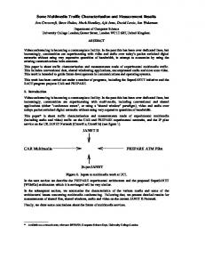
In this section we describe the Nomadic π-calculi informally. We begin by recapitulating from [SWP99] an example program in the low-level calculus showing how an applet server can be expressed. ?[a s] → * getApplet? create b = migrate to s → !b | B) (ha@s0 iack! in 0 It can receive requests for an applet on the channel named getApplet; the requests contain a pair (bound to a and s) consisting of the name of the requesting agent and the name of the site for the applet to go to. When a request is received the server creates an applet agent with a new name bound to b. This agent immediately migrates to site s. It then sends an acknowledgement to the requesting agent a (which is assumed to be on site s0 ) containing its name. In parallel, the body B of the applet commences execution. The example illustrates the main entities of the calculi: sites, agents and channels. Sites should be thought of as physical machines or, more accurately, as instantiations of the Nomadic Pict runtime system on machines; each site has a unique name. Sites are ranged over by s. Nomadic π-calculi do not explicitly address questions of network failure and reconfiguration, or of security. Sites are therefore unstructured; neither network topology nor administrative domains are represented in the calculi. Agents are units of executing code; an agent has a unique name and a body consisting of some process; at any moment it is located at a particular site. We let a and b range over agent names. Channels support communication within agents, and also provide targets for inter-agent communication — an inter-agent message will be sent to a particular channel within the destination agent. Channels are ranged over by c. New agents and channels can be created dynamically. The low-level Nomadic Pict language is built above asynchronous messaging, both within and between sites. In the current implementation inter-site messages are sent on TCP connections, created on demand, but its algorithms do not depend on the message ordering that could be provided by TCP. !b is characteristic of the low-level calculus. It is locationThe inter-agent message ha@s0 iack! dependent — if agent a is in fact on site s0 then the message b will be delivered, to channel ack in a; otherwise the message will be discarded. In the implementation at most one inter-site message is sent.
18
2.2.1
CHAPTER 2. BACKGROUND
Types
We require a type system for Nomadic π-calculi for two reasons, the first being its usual purpose: to prevent the occurrence of execution errors during the runtime of a program. Typing infrastructure algorithms requires an expressive type system, including primitive types employed in programming languages (eg. booleans, integers, strings and tuples), as well as parametric polymorphism [PS97], since an infrastructure must be able to forward messages of any type (see the message and deliver channels in Figure 2.3). The second reason is more specific: we require a type system which provides proof techniques that can be used for proving infrastructure correct. We include input/output and static/mobile subtyping, used in deriving computation steps which are functional (see Section 6.2.2) and in composing processes that are related by translocating operational relations. For the calculi to be tractable, we aim at a type system which is small, yet sufficient for the above requirements. We take the rich type system of the Pict language [PT00] as our starting point, discarding many features which, though useful for programming (eg. recursive types and record subtyping), are likely to cause complication. We also exclude complex data structures, such as maps, which are required for expressing infrastructures, but can be expressed as an encoding (see Section 6.5). We take an finite set T V of type variables of type variables, ranged over by X and Y , and a set T , ranged over by B, of base types provided by the standard libraries of Nomadic Pict. These base types includes Int, and Bool. The types defined for Nomadic π, ranged over by T , are generated by the following grammar. T
::= B
base type
| Site
site
| AgentZ | ^I T
agent
| [T1 . . . Tn ]
tuple
| X
type variable
| {|X|} T
existential
channel type
Channels and agent types are refined by annotating them with capabilities. As in [PS96], channels can be used for input only r, output only w, or both rw; these capabilities induce a subtyping order. In addition, agents are either static s, or mobile m, as in [CGG99]. Agent and channel capabilities are ranged over by Z and I respectively. We define a relation ≤ on types and stipulate that a name x of type S can be used in the context where a name of type
2.2. NOMADIC π-CALCULI
19
T is required if and only if S ≤ T . The formal definition of this relation is given in Section 3.2. Note that we do not provide bounded quantification, which mixes subtyping with polymorphism, as in the type system of Pict. Bounded quantification allows the abstract type X of an existential type {|X ≤ S|} T to be specified as a subtype of S, without revealing the exact type of X. This gives rise to great expressive power at the cost of meta-theoretic complexity. We therefore discard this feature. The type variable X in {|X|} T binds in T ; we work up to alpha conversion of bound type variables. The set of free type variables of a type T , written fv(T ), is defined as follows: def
fv(B)
=
fv(AgentZ )
def
^I T ) fv(^
def
fv([T1 . . . Tn ])
2.2.2
=
∅ ∅
=
fv(T )
def
fv(T1 ) ∪ . . . ∪ fv(Tn )
=
fv(X) fv(Site) fv({|X|} T )
def
=
X
def
∅
=
def
=
fv(T )/{X}
Type contexts
We work with located type contexts, ranged over by Γ, ∆, . . ., which assign types to names, but also specify the site where each declared agent is located. The syntax is given below: Γ
def
=
• | Γ, X | Γ, x : AgentZ @s | Γ, x : T
T 6= AgentZ
An example of a located type context is given below. s : Site, s0 : Site, c : ^ rw Int, a : Agentm @s, b : Agents @s0 The located type context declares two sites, s and s0 , and a channel c, which can be used for sending or receiving integers. It also declares a mobile agent a, located at s, and a static agent b, located at s0 . In Nomadic π-calculi, names of type AgentZ and ^ I T can be dynamically created, we may refer to such names and types as being extensible. Correspondingly, a located type context is said to be extensible if it contains no type variables and all names are of extensible types. Such type contexts can be used for binding names to located processes (see later) and can be extruded by channel communication. Located type contexts are not only useful in typechecking, but also contain site annotations, for use in the operational semantics, and consequently in the operational relations. We refer
20
CHAPTER 2. BACKGROUND
to located type contexts as location contexts whenever we wish to emphasise the presence of site annotations. The domain, range and free variables of a located type context Γ, denoted dom(Γ), range(Γ), and fv(Γ), are defined as follows. dom(•) dom(Γ, X) dom(Γ, x :
AgentZ @s)
dom(Γ, x : T ) range(•)
=
∅
def
=
dom(Γ) ∪ {X}
def
=
dom(Γ) ∪ {x}
def
=
dom(Γ) ∪ {x}
def
∅
=
def
range(Γ, X) range(Γ, x :
def
AgentZ @s)
range(Γ, x : T ) fv(Γ)
=
range(Γ)
def
=
range(Γ) ∪ {s}
def
=
range(Γ) ∪ fv(T )
def
dom(Γ) ∪ range(Γ)
=
Although located type contexts are defined as lists, the order in which the binders appears in a list is not always important. We define ≡ to be an equivalence relation between located type contexts closed under the following rules: ≡ Γ1 , Y, X, Γ2
Γ1 , X, Y, Γ2 Γ1 , X, x :
AgentZ @s,
≡ Γ1 , x :
Γ2
X 6= Y
AgentZ @s,
X, Γ2
≡ Γ1 , x : T, X, Γ2
Γ1 , X, x : T, Γ2
≡ Γ1 , x2 : T2 , x1 : T1 , Γ2
Γ1 , x1 : T1 , x2 : T2 , Γ2 Γ1 , x1 :
AgentZ1 @s1 ,
Γ1 , x1 :
AgentZ @s,
x2 :
X 6∈ fv(T )
AgentZ2 @s2 ,
Γ2 ≡ Γ1 , x2 :
AgentZ2 @s2 ,
x1 :
x1 6= x2 Z Agent 1 @s1 , Γ2
x1 6= x2 , x1 6= s2 , x2 6= s1 x2 : T, Γ2
≡ Γ1 , x2 : T, x1 : AgentZ @s, Γ2 x1 6= x2 , x2 6= s
A located type context Γ is said to extend Ξ (denoted Γ ≥ Ξ) if there exists Ξ0 such that Γ ≡ Ξ, Ξ0 ; in this case, we denote Ξ0 by Γ/Ξ.
2.2.3
Values, Patterns and Expressions
We let t range over constants — that is the members of any base type B. We assume that the sets |B|, X and T V are disjoint from each other and from all products. Channels allow communication of first-class values v, which can be constants, names, tuples and existential packages. Values can be decomposed by the receiver through the use of patterns p. Patterns
2.2. NOMADIC π-CALCULI
21
are of similar shape as values, with an addition of a wildcard pattern , allowing matching of any value. v ::= t | x | [v1 . . . vn ] | {|T }| v p ::=
| x | [p1 . . . pn ] | {|X|} p
We assume that p contains no duplicated names or type variables and that X is binding in {|X|} p. An existential package reveals the type which is bound in the existential type. For example, if c is a channel of type ^ rw Int, an existential package {|Int|} [c 5] has the type ^rw X X]; the package reveals the type variable X as Int. If d is a channel of T = {|X|} [^ type ^ rw Bool then, a package {|Bool|} [d true true] is also of type T . A polymorphic server may use an existential pattern {|X|} [x y] for decomposing such existential packages, so that eg. the value matching y can be sent along the channel matching x. The value grammar is extended with some basic functions to give expressions, ranged over by ev. Basic functions, ranged over by f , include arithmetic operations and equality tests. ev ::= t | x | [ev1 . . . evn ] | {|T }| ev | f (ev1 , . . . , evn ) The set of all basic functions, denoted F, is intended to include most functions which are provided by Nomadic Pict libraries. For the time being, however, we restrict the basic functions to maps from tuples of base types to a single base type — except for equality where names of any type can be compared. Expressions are computed locally (in let processes) and, as for values, can be matched using patterns. The evaluation relation eval(ev) defined over expressions is given inductively as follows: eval(t) eval(x) eval([ev1 . . . evn ]) eval({|T }| ev) eval(f (ev1 , . . . , evn ))
def
=
def
=
def
t x
=
[eval(ev1 ) . . . eval(evn )]
def
{|T }| eval(ev)
=
def
=
f (eval(ev1 ), . . . , eval(evn ))
We stipulate that all functions f ∈ F must be total functions (ie. if f maps tuples of type (B1 , . . . , Bn ) to base type B then, for any t1 ∈ B1 , . . . , tn ∈ Bn , f (t1 , . . . , tn ) is defined, and is of type B). This ensures that evaluation of an expression always yields a reduction (see Section 4.4).
22
2.2.4
CHAPTER 2. BACKGROUND
Processes
We formulate two forms of processes: basic and located processes. Basic processes describe the threads of execution within each agent, and located processes describe the overall state of the computation in which many agents may be concurrently executing. In this section, we give the syntax for basic and located processes. This section is substantially a recapitulation of [SWP99].
Basic Processes The syntax of basic process for the low-level calculus is given below: P
::= 0 | P |Q | new c : ^ I T in P !v | c? ?p→ P | * c? ?p→ P | c! | if v then P else Q
� π-calculus primitives conditional
| let p = ev in P | create Z a = P in Q | migrate to s → P
let declaration
!v then P else Q | iflocal haic!
inter-agent communication
!v | ha@sic! !v | haic!
sugared outputs
creation of new agent agent migration
The execution of the construct create Z b = P in Q spawns a new agent on the current site (with mobility capability Z and body P ). After the creation, Q commences execution in parallel with the rest of of the body of the spawning agent. The new agent has a unique name which may be referred to both in its body and in the spawning agent. The name b is binding in P and Q. Agent can migrate to named sites — the execution of migrate to s → P as part of an agent results in the whole agent migrating to site s. After the migration, P continues in parallel with the rest of the body of the agent. The body of an agent consists of several basic processes in parallel — essentially many threads. It uses π-calculus style interaction primitives. Execution of new c : ^I T in P creates a new unique channel name c (accessible in I mode) for carrying values of type T ; c is binding in !v (of value v on channel c) and an input c? ?p → P in the same agent may P . An output c! synchronise, resulting in P with the appropriate parts of the value v bound to the formal ?p → P behaves similarly except that it parameters in the pattern p. A replicated input * c? remains after the synchronisation, and so may receive another value. The conditional process if v then P else Q allows the boolean value v to be tested for its truth value and selects a continuation process accordingly. The execution of the construct let p = ev in P evaluates expression ev and triggers P with the appropriate parts of the evaluated value eval(ev)
2.2. NOMADIC π-CALCULI
23
?p → P , * c? ?p → P and let p = ev in P bound to the formal parameters in the pattern p. In c? the names in p are binding in P . Finally, the low-level calculus includes a single primitive for interaction between agents. The !v then P else Q in the body of agent b has two possible outcomes. execution of iflocal haic! !v will be delivered to a (where If the agent a is on the same site as agent b then the message c! it may later interact with an input) and P will commence execution in parallel with the rest of the body of b; otherwise the message will not be delivered and Q will execute as part of b. The construct is analogous to test-and-set operations in shared memory systems—delivering the message and starting P , or discarding it and starting Q, atomically. It can greatly simplify algorithms that involve communication with agents that may migrate away at any time, yet is still implementable locally, by the runtime systems on each site. We can express !v and ha@sic! !v attempt two other useful constructs in the language introduced so far: haic! !v to agent a, on the current site and on s, respectively. They fail silently if a is to deliver c! not where it is expected to be and so are usually used only where a is predictable. They can be translated into the core calculus as follows. !v haic!
def
!v ha@sic!
def
!v then 0 else 0 = iflocal haic!
migrate to s → haic! !v) in 0 = create m b = (migrate
b 6∈ fv(a, c, v, s)
We also introduce the following abbreviations. !v then P iflocal hbic! let x1 = v1 , . . . , xn = vn in P new x1 : T1 , . . . , xn : Tn in P
def
!v then P else 0 = iflocal hbic!
def
= let x1 = v1 in . . . let xn = vn in P
def
= new x1 : T1 in . . . new xn : Tn in P
In the execution of iflocal a new channel name can escape the agent where it was created, !v and an later to be used for output and/or input. Synchronisation of a local output c! ?x→ P only occurs within an agent, however. Consider for example the process below, input c? executing as the body of an agent a. create m b = ?x → (x! !3|x? ?n→00) c? in new d : ^ rw Int in !d then 0 iflocal hbic! !7 | d! It has a reduction for the creation of agent b, a reduction for the iflocal that delivers !d to b, and then a local synchronisation of this output with the input on c. the output c!
24
CHAPTER 2. BACKGROUND
!7 and agent b has body d! !3|d? ?n→00. Only the latter output on d Agent a then has body d! ?n→00. For each channel name there is therefore effectively can synchronise with b’s input d? a π-calculus-style channel in each agent. The channels are distinct, in that outputs and inputs can only interact if they are in the same agent. At first sight this semantics may seem counter-intuitive, but it reconciles the conflicting requirements of expressiveness and simplicity of the calculus.
High-Level Calculus The high-level calculus adds a single location-independent commu!v to the low-level calculus. nication primitive ha@?ic! P
!v ::= ha@?ic!
High level: LI output
!v to The intended semantics of this is that its execution will reliably deliver the message c! agent a, irrespective of the current site of a and of any migrations. The low-level communication primitives are also available for interaction with application agents whose locations are predictable.
Located Processes
The syntax of located processes, ranged over by LP , of low- and
high-level calculi is as follows. LP ::= @a P | LP |LQ | new x : AgentZ @s in LP | new x : ^ I T in LP Here the body of an agent a may be split into many parts. It may, for example, be written as @a P1 | . . . |@a Pn . Only channels and agents (and not sites) can be created dynamically; the construct new x : AgentZ @s in LP declares a new agent x (binding in LP ), located at site s. A new channel can be created similarly, although such a channel is not located. We define nπLD,LI be the set of high-level located processes defined by the above grammar. The set of low-level located processes, nπLD , can be obtained from nπLD,LI by excluding process terms which contain LI primitives. There are two extreme possibilities for annotating location information to process terms. In one, a locator is applied to the largest possible unit, with all co-located subterms gathered into a single subterm (as in [CG98, SV99]). The other extreme is where every elementary subterm ?b → @b P . This latter approach is adopted by dpi [Sew98], whose is explicitly located, eg. @a c? reduction semantics allows communication between inputs and outputs which are located at different locations. The former approach is too restrictive for Nomadic π-calculi, and makes labelled transitions and operational equivalences difficult to define. The latter approach is flexible, but it contains redundant location information — some of which might not be easily
2.3. CENTRALISED SERVER TRANSLATION
25
?p → @b P . In our case, structural congruence implementable or desirable, for example @a c? rules (Str-Distr) and (Str-N-Extrude), defined in Section 4.1, are used for projecting location information down to elementary subterms if needed.
Free and Bound Variables The free variables of P and LP denoted by fv(P ) and fv(LP ) are defined as those names and type variables which are not bound in let patterns, input patterns or new declaration. All bound names are subjected to alpha-conversion.
2.3
Centralised Server Translation
In this section, we present an infrastructure algorithm, expressed as translation from the source language nπLD,LI to the target language nπLD .
This algorithm, based on the sim-
plest algorithm from [SWP99], is a central-forwarding-server algorithm. It uses a centralised daemon for keeping a record of all existing agents. Location-independent messages are sent to the daemon, which forwards such messages to their destination. Before an agent migrate, it informs the daemon and wait for an acknowledgement; this ensures that all messages forwarded from the daemon are delivered before the agent migrates away. After the migration, the agent tells the daemon it has finished moving and continues. When a new agent is created, the new agent registers with the daemon, telling its site. The new agent, as well as its parent, wait for an acknowledgement from the daemon before they continue. Locks are used to ensure, for example, that an agent will not migrate away while a message forwarded by the daemon is on its way. The algorithm has been chosen to illustrate the model, the use of the calculi, and, most importantly, the proof of correctness. Algorithms used in the actual mobile agent systems would have to be more delicate, taking into account efficiency as well as robustness under partial failure. The original algorithm has been modified in the following ways to simplify the correctness proof. • Type annotations have been added and checked with the Nomadic Pict type checker [Woj00a] (although this does not check the static/mobile subtyping). • The algorithm is more serialised; eg. releasing deliver at last moment, so that the newly-created agent is more deterministic.
26
CHAPTER 2. BACKGROUND • Fresh channels are used for transmitting acknowledgements, making such channels linear [KPT96]. This simplifies the proof of correctness, since communication along a linear channel yields an expansion. • The translation is extended to arbitrary located processes (not just source programs containing a single agent). Proving operational relations involves using co-inductive proof techniques. This means that, instead of defining the translation for programs containing a single agent, we need to strengthen it so that any program can be translated.
The daemon is itself implemented as a static agent. The translation CΦ [[LP ]] of a located process LP = new ∆ in (@a1 P1 | . . . | @an Pn ) (well-typed with respect to Φ) then consists roughly of the daemon agent in parallel with a compositional translation [[Pi ]]ai of each source agent; or more precisely: CΦ [[LP ]]
def
=
new ∆, Φaux , m : Map[Agents Site] in !m | makeMap(m; Enlist(Φ, ∆))) @D (Daemon | lock! Q !si | Deliverer) | i∈{1...n} @ai ([[Pi ]]ai | currentloc!
(†)
where each agent ai is distinct and assumed to be located at si and Enlist(Φ, ∆) initialises a site map: a finite map from agent names to site names, recording the current site of every agent a1 . . . an in the system — both free and bound. It is defined recursively below. Enlist(•) Enlist(x : AgentZ @s, Θ) Enlist(x : T, Θ)
def
= nil
def
=
def
=
:: Enlist(Θ) [x z]: Enlist(Θ)
T 6= AgentZ
The makeMap(m; ls) function, defined in Section 6.5, can then be used for generating a basic process representing the site map, accessible via m. The body of the daemon and the compositional translation are shown in Figures 2.3 and 2.4. They interact using channels of an interface context Φaux , also defined in Figure 2.3. The interface context additionally declares lock channels and the daemon name D, located at a fixed site SD. The daemon uses a map type constructor, which (together with the map operators) can be translated into the core language (see Section 6.5). The process definitions on the right in Figures 2.3 and 2.4 (such as mesgQ, regReq, and regBlockC) are used extensively for defining various constructs used for the correctness proof in Chapter 7.
2.3. CENTRALISED SERVER TRANSLATION
27
def
Daemon = ? {|X|} [a c v] → * message? ?m → lock?
(mesgReq({|X|} [a c v]))
lookup lookup[Agents
Site] a in m with new dack : ^ rw [] in found found(s) →new ! {|X|} [c v dack] ha@sideliver!
?[] → lock! !m | dack? notfound →00 ?[b s rack] → | * register? ?m → lock? let let[Agents ! m0 (lock!
(regReq(b s rack))
m0
= (m with b 7→ s) in ![]) | hb@sirack!
Site]
?[a mack] → | * migrating? ?m → lock?
(migReq(a mack))
lookup lookup[Agents
Site] a in m with new migrated : ^ rw [Site ^ w []] in found found(s) →new ![migrated] ha@simack! ?[s0 ack] → | migrated? let m0 = (m with a 7→ s0 ) in
(migProc(a m migrated))
!m0 | ha@s0 iack! ![]) (lock! notfound →00 Φaux
def
=
D : Agents @SD, lock : ^ rw Map[Agents Site], register : ^ rw [Agents Site ^ w []], ^w [Site ^ w []]]], migrating : ^ rw [Agents ^ w [^ message : ^ rw {|X|} [Agents ^ w X X], ^w X X ^ w []], deliver : ^ rw {|X|} [^ currentloc : ^ rw Site
Figure 2.3: The Central Server Daemon and the Interface Context
28
CHAPTER 2. BACKGROUND
def
!v]]a [[hb@?ic!
=
! {|T }| [b c v] hD@SDimessage!
� � def create Z b = P in Q a = ?s →new new pack : ^ rw [], rack : ^ rw [] in currentloc? create Z b = ![b s rack] hD@SDiregister! ?[] →iflocal iflocal haipack! ![] then | rack?
(regBlockC(s pack rack P ))
!s | [[P ]]b | Deliverer) (currentloc! in ?[] → (currentloc! !s | [[Q]]a ) pack? where
Deliverer
def
=
(regBlockP(s pack Q))
? {|X|} [c v dack] → (hD@SDidack! ![] | c! !v) * deliver?
def
migrate to s → P ]]a [[migrate = ? →new new mack : ^ rw [^ ^w [Site ^ w []]] in currentloc? ![a mack] hD@SDimigrating! ?[migrated] → | mack? migrate to s → new ack : ^ rw [] in ![s ack] (hD@SDimigrated!
(migBlock(s mack P )) (migReady(s migrated P ))
?[] → currentloc! !s | [[P ]]a ) | ack? [[00]]a
def
[[P |Q]]a
def
=
[[P ]]a | [[Q]]a
?p → P ]]a [[c?
def
?p → [[P ]]a c?
*c? ?p → P ]]a [[*
def
= 0 =
?p → [[P ]]a = * c?
def
!v]]a [[c!
=
iflocal hbic! !v then P else Q]]a [[iflocal � � I new x : ^ T in P a if v then P else Q]]a [[if let p = ev in P ]]a [[let
!v c!
def
!v then [[P ]]a then [[Q]]a = iflocal hbic!
def
= new x : ^ I T in [[P ]]a
def
= if v then [[P ]]a then [[Q]]a
def
= let p = ev in [[P ]]a
Figure 2.4: The Compositional Encoding
2.3. CENTRALISED SERVER TRANSLATION
29
The daemon consists of three replicated inputs, on the message, register, and migrating channels, ready to receive messages from the encodings of agents. Reacting to such messages Daemon produces one of the following request processes: • a registration request, regReq(b s ack): an agent b requests to be registered with an initial site s; • a migrating request, migReq(a ack): an agent a requests permission to migrate; and • a message forwarding request, mesgReq({|T }| [a c v]): an agent requests the daemon to !v to agent a. forward a message c! In making registration and migrating requests, the requesting agent needs to supply a fresh channel ack which the daemon can use for sending acknowledgement once the request has been processed. Part of the initialisation code places Daemon in parallel with an output on lock which carries a reference to the site map of the daemon. This ensures that the daemon is essentially singlethreaded, since each of the above requests begins with an input on lock (thereby acquiring both the lock and the site map), and does not relinquish the lock until the daemon finishes with the request. The code preserves the invariant that at any time there is at most one output on lock. Each agent records its current site internally as an output on its currentloc. This channel is also used as a lock, to enforce mutual exclusion between the encodings of all agent creation and migration commands within the body of the agent. The local lock is not essential for the correctness of the algorithm but it makes the proof of correctness simpler, since the lock ensures that at anytime an agent can be involved with at most one request to the daemon. This simplifies the intermediate language (see Section 7.2), as well as working with partially committed agents. If an agents could involve with more than one daemon requests, committing its partially committed actions (as in Section 7.4) can be problematic: at which site would an agent involved with several migration requests be placed when committed, for example. Turning to the compositional translation [[.]], it is defined inductively on the syntax of basic processes, allowing properties of [[.]] to be proved by induction. Only three clauses, shown in Figure 2.4, are non-trivial: for the location-independent output, agent creation and agent migration primitives. For the rest, [[.]] is homomorphic. We assume in the definition that none of the names in typewriter font (which, by convention, are auxiliary names defined in � � Φaux ) occur in x (for the definition of new x : ^ I T in P a ) and in p (for the definitions of
30
CHAPTER 2. BACKGROUND
processes containing pattern p).
!v to agent b) Location-Independent Output An LI output in an agent a (of message c! is implemented simply by using a location-dependent (LD) output to send the message to channel message at the daemon, as an existential package with a triple [b c v]. Reacting to the message on message, the daemon produces a message forwarding request mesgReq({|T }| [b c v]) (T being the type of v) which competes with other requests in acquiring the output on lock. Once successful, it looks up the target agent’s site in the acquired site map, creates a fresh channel dack and forwards the message in LD mode (together with dack) to the deliver channel of b. In each agent, the deliver channel is handled by a Deliverer !v message process, as in Figure 2.4. This reacts to deliver messages by emitting a local c! and acknowledging the daemon (again using LD communication) via dack. Meanwhile no agent may migrate before the deliver message arrives, since the daemon is single-threaded and waits for such an acknowledgement before releasing lock. Note that the notfound branch of the lookup will never be taken as the algorithm ensures that all agents register before messages can be sent to them. Following [SWP99], the inter-agent communications involved in the delivery of a single location-independent output are illustrated below.
a
D
b
!{|T }| [b c v] message! !{|T }| [c v dack] deliver! ![] dack!
Creation In order for the daemon’s site map to be kept up-to-date, agents must register with the daemon, telling it their site. They must do this both upon creation and after migration. The encoding of create Z b = P in Q (in Figure 2.4) first acquires the local lock and current site s and then creates the new agent b, as well as fresh channels pack and rack. The body of b sends a register message to the daemon, supplying rack. When Daemon at D receives a register message, it produces a registration request process regReq(b s rack) which competes with other requests in acquiring the output on lock. Upon success, the daemon updates the site map and then uses rack to acknowledge the registration of b. Meanwhile b may not begin executing before the acknowledgement arrives; this prevents b from sending a migration request to the daemon before it is registered.
2.3. CENTRALISED SERVER TRANSLATION
31
After the acknowledgement is received from the daemon, b sends an acknowledgement to a using pack, initialises the local lock of b with s, installs a Deliverer, and allows the encoding of the body P of b to proceed. Meanwhile, the local lock and the encoding of the continuation process Q is kept until the acknowledgement via pack is received. This prevents the encoding of Q from using the daemon to forward LI messages to b before b is registered. The inter-agent communications involved in the creation of a single agent are illustrated below. a
D
b
create ![b s rack] register! ![] rack! ![] pack!
Migration
The encoding of a migrating process in a (also in Figure 2.4) first acquires
the output on currentloc at a (discarding the current site data). It then creates a fresh channel mack and sends a migrating message to the daemon with a tuple [a mack]. The encoding becomes migBlock(s mack P ), waiting for the daemon to send a message to mack before proceeding with the migration. This ensures that if the daemon is sending a message on deliver channel to a (ie. forwarding an LI output), then such a message will arrive before a migrates away. Reacting to the message on migrating message, Daemon produces a migrating request process migReq(a mack) which tries to acquire the lock and the current site map. Once it succeeds, it looks up the current site of a in the acquired map m, creating a fresh channel migrated and sending it (using an LD primitive) to a along channel mack. The request process at the daemon now becomes migProc(a m migrated), waiting for the requesting agent to complete its migration. The blocked agent migBlock(s mack P ), once it receives a message from mack, migrates agent a to the new site s, then creates a fresh channel ack and sends a tuple [s ack] to the daemon via channel migrated (using an LD primitive). Meanwhile, the local lock and the encoding of the continuation process P is kept until the acknowledgement via ack is received from the daemon. Finally, the blocked daemon migProc(a m migrated) receives a message on migrated, updates the site map, then relinquishes the lock and then sends an acknowledgement to a at its new site. The inter-agent communications involved in the migration of a single agent are illustrated below.
32
CHAPTER 2. BACKGROUND
a
D ![a mack] migrating! ![migrated] mack!
migrate to ![s ack] migrated! ![] ack!
Located Processes The definition of top-level encoding given in Equation (†) is restricted to certain forms of located processes. We may arrange an arbitrary located process into the desired form using the following translation. [[@a P ]] [[LP1 | LP2 ]] new ∆ in LP ]] [[new
(A1 � A2 )(a)
def
=
def
=
def
(•; a 7→ P ) (∆1 , ∆2 ; (A1 � A2 ))
=
(∆, Θ; A)
def
A (a) | A2 (a) 1 A1 (a) A (a)
=
2
where [[LPi ]] = (∆i ; Ai )
where [[LP ]] = (Θ; A) a ∈ dom(A1 ) ∩ dom(A2 ) a ∈ dom(A1 ) ∧ a 6∈ dom(A2 ) a ∈ dom(A2 ) ∧ a 6∈ dom(A1 )
It is not difficult to prove that indeed LP ≡ new ∆ in
Q
a∈dom(A) A(a)
where [[LP ]] = (∆; A).
Chapter 3
Type System This chapter presents our type system for Nomadic π-calculi. We first give the typing judgements for different syntactic constructs in Section 3.1. Sections 3.3-3.6 give the axioms and inference rules for these typing judgements. We state some properties of the type system in Section 3.7. In Section 3.8, we define type-preserving substitutions, and prove that they preserve typability of processes. We also show that matching a value and a pattern of the same type yields a type-preserving substitution.
3.1
Forms of Typing Judgement
The richness of our type system (subtyping and polymorphism, in particular) leads us away from using the notion of sorting [Mil93b]. Taking into the consideration the rigorous programming language-like syntax of Nomadic π-calculi, we take as our starting point the style used in the definition of the programming language Pict [PT00]. We define typing judgements for different syntactic categories. The type system of Nomadic π-calculi consists of of axioms and inference rules defining sets of derivable typing judgements of the following forms: `Γ
unlocated type context Γ is well-formed.
`L Γ
located type context Γ is well-formed.
Γ`S≤T
S is a subtype of T under assumptions Γ.
(SubT-*)
Γ`T
type T is well-formed under assumptions Γ.
(Type-*)
Γ ` x@s
the name x is located at s under assumptions Γ.
(Var-Loc)
Γ`p∈T .∆
pattern p requires type T and yields bindings ∆.
(Pat-*)
33
(C-*) (L-C-*)
34
CHAPTER 3. TYPE SYSTEM
Γ`e∈T
value or expression e has type T under assumptions Γ.
Γ `a P
basic process P as part of agent a is well-formed under assumptions Γ.
Γ ` LP
located process LP is well-formed under assumptions Γ.
(Expr-*)
In this thesis, type contexts are always located. Apart from the judgements of the form `L Γ and Γ ` x@s, however, we discard the site annotations in located type contexts, and work with unlocated type contexts when dealing with the above typing judgements. This avoids having to assign “dummy” annotations in typechecking pattern variables of type AgentZ (see (Pat-Var)).
3.2
Subtyping Rules
The subtyping relation is built from the following order of capability tags: r
s
w rw
m
The subtyping relation is defined by a rule for each type constructor or constant, as given in Figure 3.1. (SubT-Base)
(SubT-Var)
(SubT-Site)
Γ`B
Γ`X
`Γ
Γ`B≤B
Γ`X≤X
Γ ` Site ≤ Site
(SubT-Chan) I = I 0 = rw ⇒ (Γ ` S ≤ T ∧ Γ ` T ≤ S)
(SubT-Agent) `Γ
Z ≤ Z0
I ≤ I0 = r Z0
Γ ` AgentZ ≤ Agent
I≤
I0
=w
⇒Γ`S≤T ⇒Γ`T ≤S I0
Γ ` ^I S ≤ ^ T (SubT-Exist)
(SubT-Tuple)
Γ, X ` S ≤ T
Γ ` S1 ≤ T 1
Γ ` {|X|} S ≤ {|X|} T
Γ ` [S1 . . . Sn ] ≤ [T1 . . . Tn ]
...
Γ ` Sn ≤ T n
Figure 3.1: Rules for subtyping Base types, site type and type variables are simply subtypes of themselves (SubT-Base, SubT-Var and SubT-Site). Agent subtyping is simple as Agent is simply a type not a
3.3. TYPE AND TYPE CONTEXT FORMATION
35
constructor. Since mobile agents are more capable than static agents, we take Agentm ≤ Agents (SubT-Agent). The rule (SubT-Chan) shows the channel constructor ^ r covariant in its argument, whereas ^ w contravariant, as in [PS96]. Operationally, this captures the observation that: if a given channel c is used only to read elements of type T then it is safe to replace c by another channel c0 carrying elements of type S, as long as any element that is read from c0 may safely be regarded as an element of T — that is, as long as S is a subtype of T . The constructor ^ rw is invariant in the subtype relation (i.e. ^ rw S is a subtype of ^ rw T only when S and T are equivalent — ie. identical in our calculi). The type ^ rw T is a subtype of both ^ r T and ^ w T . That is, we are allowed to forget either the capability to write or the capability to read on a channel: a channel that can be used for both input and output may be used in a context where just one capability is needed. Other type constructors are covariant. A tuple S is a subtype of another tuple T whenever S and T contain exactly the same number of elements and the types of the corresponding elements are also subtypes (SubT-Tuple). An existential type {|X|} S is a subtype of of {|X|} T if S is a subtype of T , with X being a part of the assumption (SubT-Exist).
3.3
Type and Type Context Formation
The rules for unlocated type context formation are given in Figure 3.2. They ensure that none of the declared type variables and names are duplicated, and that each type in the binding is well-formed. To typecheck located type contexts, we also need to ensure the validity of site annotations. The rules for located type context formation are similar to those for unlocated type contexts, replacing the rule (C-Var) by (L-C-Var) and (L-C-Agent). Such rules are given in Figure 3.3.
(C-Empty) `•
(C-TVar)
(C-Var)
` Γ X 6∈ dom(Γ)
`Γ
` Γ, X
` Γ, x : T
Γ`T
x 6∈ dom(Γ)
Figure 3.2: Rules for unlocated type context formation The rules for type formation are given in Figure 3.4. They are standard; we omit their explanation.
36
CHAPTER 3. TYPE SYSTEM
(L-C-TVar)
(L-C-Empty)
`L Γ X 6∈ dom(Γ)
`L •
`L Γ, X
(L-C-Var) `L Γ T 6= AgentZ
Γ`T
x 6∈ dom(Γ)
`L Γ, x : T (L-C-Agent) `L Γ
Γ ` s ∈ Site
`L Γ, x :
Γ ` AgentZ
x 6∈ dom(Γ)
AgentZ @s
Figure 3.3: Rules for located type context formation
(Type-Base)
(Type-Site)
(Type-Agent)
`Γ
`Γ
` Γ Z ∈ {m, s}
Γ ` Site
Γ ` AgentZ
B∈T
Γ`B (Type-Exist)
(Type-Var)
Γ, X ` T
` Γ X ∈ dom(Γ)
X 6∈ dom(Γ)
Γ ` {|X|} T
Γ`X
(Type-Chan)
(Type-Tuple)
Γ`T
Γ ` T1
Γ`
^I T
I ∈ {r, w, rw}
...
Γ ` Tn
Γ ` [T1 . . . Tn ] Figure 3.4: Rules for type formation
3.4. VALUES AND EXPRESSIONS
3.4
37
Values and Expressions
Due to their shared structure, the same set of judgement rules are used for both values and expressions. We let e range over values and expressions. The rules are given in Figure 3.5. (Expr-BVal)
(Expr-Sub)
Γ0
`Γ t∈B
Γ`e∈S
`x∈T
Γ`t∈B
Γ`e∈T
(Var-Id) ` Γ, x : T, Γ, x : T,
Γ0
(Expr-Exist) Γ ` e ∈ {S/X}T
Γ`S≤T
(Expr-Tuple) Γ`S
Γ ` {|S|} e ∈ {|X|} T
Γ, X ` T
Γ ` e1 ∈ T1
...
Γ ` en ∈ Tn
Γ ` [e1 . . . en ] ∈ [T1 . . . Tn ]
(Equality) Γ`e∈T
Γ ` e0 ∈ T
Γ ` e = e0 ∈ Bool (Eval) f ∈F
f is not =
f : B1 × . . . × Bn → B
Γ ` e1 ∈ B1 . . . Γ ` en ∈ Bn
Γ ` f (e1 , . . . , en ) ∈ B Figure 3.5: Rules for value and expression formation If the type context contains the binding x : T then the type of x is T in this context (Var-Id) (all binding names are unique — ensured by the precondition, so there is no ambiguity in this rule). Constants of base types simply possess such types (Expr-BVal). The subsumption rule (Expr-Sub) allows types of values to be promoted in the subtype relation: if e is a value of type S and S is a subtype of T then e is also of type T . A expression {|S|} e is an existential package of type {|X|} T if the “witness type” S is wellformed, and the actual type of the expression e must match the type T after the substitution of S for X. Readers familiar with typed λ-calculi will recognise the similarity of this rule to the standard introduction rule for existential types (cf. [MP88]). We prevent the escape of the hidden type variable rule by the second and third assumptions of (Expr-Exist), ensuring that X is not in the domain of Γ and hence not free in S. If the expressions e1 through en have the type T1 through Tn then the tuple expression [e1 . . . en ] has the tuple type [T1 . . . Tn ] (Expr-Tuple). To typecheck a function application
38
CHAPTER 3. TYPE SYSTEM
expression f (e1 , . . . , en ), we look up the type of the function f , typecheck each argument expression according to the argument type obtained, and the type of the whole expression is the type of the range of f (Eval, Equality). As discussed in Section 2.2.3 on page 21, with an exception of equality test, where the arguments can be of any type, the type of each argument as well as the result must be a base type. (Var-Loc) `L Γ, x : AgentZ @s, Γ0 Γ, x : AgentZ @s, Γ0 ` x@s Figure 3.6: Rule for locating names The location of an agent can be looked up using (Var-Loc) in Figure 3.6. This judgement form Γ ` a@s is not employed in typechecking, but is essential in the operational semantics.
3.5
Patterns
Pattern typing statements have the form Γ ` p ∈ T . ∆, ie. each pattern has a type, describing the values it can match, and moreover gives rise to a set of extra bindings ∆. Their rules are given in Figure 3.7. (Pat-Var)
(Pat-Tuple)
`Γ
Γ ` p1 ∈ T 1 . ∆ 1
Γ`T
...
Γ ` pn ∈ T n . ∆ n
Γ`x∈T .x:T
Γ ` [p1 . . . pn ] ∈ [T1 . . . Tn ] . ∆1 , . . . , ∆n
(Pat-Wild)
(Pat-Exist)
`Γ
Γ, X ` p ∈ T . ∆
Γ`T
Γ` ∈T .•
X 6∈ dom(Γ)
Γ ` {|X|} p ∈ {|X|} T . X, ∆ Figure 3.7: Rules for pattern formation
A variable pattern x and a wildcard pattern
requiring type T match any value of type T
(provided that T is a well-formed type) and gives rise to, in the case of variable pattern, a binding for the variable x (Pat-Var), and, in the case of wildcard pattern, no binding (Pat-Wild). A tuple pattern [p1 . . . pn ] requiring type [T1 . . . Tn ] is typable if each subpattern pi requiring type Ti is typable; moreover, it gives rise to a set of bindings comprising all the bindings
3.6. BASIC AND LOCATED PROCESS
39
from its subpatterns (Pat-Tuple). An existential pattern {|X|} p matches any value of type {|X|} T , where T is the type required by the pattern p (under the assumed existence of X). Such a pattern yields not only the bindings produced by p, but also the “existence of X” binding (Pat-Exist).
3.6
Basic and Located Process
The judgement rules for basic and located processes are relatively simple. Valid formation of a basic process, in addition to ensuring correct deployment of names, must also consider its ability to be located at agents — in particular, if such a process contains any possibility of migration, it cannot be located in a static agent. We give the judgement rules for basic process in Figures 3.8-3.11. (Rep-In) Γ ` x ∈ ^rT
Γ`p∈T .∆
?p→ P Γ `a x?
?p→ P and Γ `a * x?
Γ, ∆ `a P
(Out) Γ ` a ∈ Agents
Γ ` c ∈ ^wT
Γ`v∈T
!v Γ `a c! (SendLI) Γ ` a, b ∈ Agents
Γ ` c ∈ ^wT
Γ`v∈T
!v Γ `a hb@?ic! Figure 3.8: Rules for basic processes: input and output ?p → P (respectively *c? ?p → P ) is well-formed if c is a channel A (replicated) input process c? which can be used for input, ie. its type can be promoted to ^ r T for some T . The guarded process P must be well-typed with respect to the context extended with the bindings ∆, introduced by typing pattern p requiring type T (Rep-In). The typechecking rules for output processes, including the sugared LD output and LI output, are similar to each other. The !v is well-typed if c can be used for output, ie. its type can be promoted to ^ w T for message c! some T matching the type of v (Out). In case of LI outputs, we must also ensure that the agent target of the message is really an agent (SendLI). Note that, by using the subsumption rule (Expr-Sub), a mobile agent may have type Agents . The assumption Γ ` a ∈ Agents is
40
CHAPTER 3. TYPE SYSTEM
used whenever we need to ensure that a is an agent. A conditional expression is well-formed if the guard expression has boolean type and both branches of the conditional are well-formed (Cond). A let declaration let p = ev in P is well-formed if the expression is of a type T and the guarded process P is well-typed with respect to the context extended with the bindings ∆, introduced by typing pattern p requiring type T (Let).
(Cond)
(Let)
Γ ` v ∈ Bool
Γ `a P
Γ `a Q
Γ ` ev ∈ T
Γ `a if v then P else Q
Γ`p∈T .∆
Γ, ∆ `a P
Γ `a let p = ev in P
Figure 3.9: Rules for basic processes: internal computation A create Z b = P in Q expression is well-formed as part of an agent a if b is fresh and, assuming b of type AgentZ , P is well-typed as part of b and Q is well-typed as part of a (Create). Typechecking migrate to s → P as part of agent a involves checking that agent a is capable of migrating (ie. it has type Agentm ), that s is a site and that P is well-formed (Migrate). Similarly to the conditional, an iflocal expression is well-formed if the guard expression (which can be regarded as an LD output) and both branches are well-formed (IfLocal). (Create) a 6= b
Γ, b : AgentZ `b P
Γ, b : AgentZ `a Q
Γ `a create Z b = P in Q (Migrate) Γ ` a ∈ Agentm
Γ ` s ∈ Site
Γ `a P
Γ `a migrate to s → P (IfLocal) Γ ` b ∈ Agents
Γ ` c ∈ ^wT
Γ`v∈T
Γ `a P
Γ `a Q
!v then P else Q Γ `a iflocal hbic! Figure 3.10: Rules for basic processes: agent constructs A 0 process locating at a is always well-typed (Nil), provided that the type context is wellformed and that a is indeed an agent. The parallel composition of two basic processes is
3.7. BASIC PROPERTIES
41
well-formed with respect to a given context if each process is (Par). A new declaration is well-typed if the process under such declaration is well-typed with respect to the assumption extended with the new binding (LocalNew). (Par)
(Nil) `Γ
Γ ` a ∈ Agents
Γ `a P
Γ `a 0
(LocalNew) Γ, x : ^I T `a P
Γ `a Q
Γ `a new x : ^ I T in P
Γ `a P | Q
Figure 3.11: Rules for basic processes: composition
Located Process Due to the simplicity of the located process syntax, the typechecking rules for located processes (given in Figure 3.12) are straightforward. A located basic process @a P is well-formed if a is an agent and P is well-formed as part of a (At). The rules for parallel composition and channel declaration are similar to those defined for their basic process counterparts (LPar) and (NewChannel). Agent declaration is similar to channel declaration, although we also need to make sure that the site annotation attached is indeed a site (NewAgent). (At)
(LPar)
Γ `a P
Γ`a∈
Agents
Γ ` LP
Γ ` LQ
Γ ` @a P
Γ ` LP | LQ
(NewChannel) Γ, c : ^I T ` LP
(NewAgent)
Γ ` new c :
^I T
in LP
Γ, a : AgentZ ` LP Γ ` new a :
AgentZ @s
Γ ` s ∈ Site in LP
Figure 3.12: Rules for located process formation
3.7
Basic Properties
We have proved several properties of this type system, including the property that it is preserved by valid type context permutation (Lemma 3.7.1), and strengthening and weakening of type contexts (Lemma 3.7.2). We also prove that, whenever evaluation function eval(·) is defined, it preserves types. These properties are crucial for the subsequent lemmas, such as the subject reduction (Theorem 4.5.1), as well as those concerning operational relations. The proofs of these lemmas are routine inductions on type derivation; we omit their details.
42
CHAPTER 3. TYPE SYSTEM
Lemma 3.7.1 (Context permutation preserves typing) 1. If `L Γ and ∆ ≡ Γ then `L ∆. 2. If Γ `a P and ∆ ≡ Γ then ∆ `a P . 3. If Γ ` LP and ∆ ≡ Γ then ∆ ` LP . Lemma 3.7.2 (Typing: weakening and strengthening) 1. Γ ` e ∈ T and ` Γ, ∆ IFF Γ, ∆ ` e ∈ T and dom(∆) ∩ fv(e) = ∅. 2. Γ ` p ∈ T . Θ, ` Γ, ∆ and dom(∆) ∩ fv(p) = ∅ IFF Γ, ∆ ` p ∈ T . Θ and dom(∆) ∩ (fv(p) ∩ fv(T )) = ∅. 3. Γ `a P and ` Γ, ∆ IFF Γ, ∆ `a P and dom(∆) ∩ (fv(P ) ∪ {a}) = ∅. 4. Γ ` LP and ` Γ, ∆ IFF Γ, ∆ ` LP and dom(∆) ∩ fv(LP ) = ∅. Lemma 3.7.3 (Evaluation preserves types) If Γ ` e ∈ T and eval(e) is defined then Γ ` eval(e) ∈ T .
3.8
Type-Preserving Substitution and Matching
Substitutions, ranged over by σ, ρ, are finite maps associating names with values, as well as type variables with types. Substitution is extended in the natural way to an operation on processes (renaming bound names as necessary to avoid capture). We write {T1 /X1 , . . . , Tn /Xn , v1 /x1 , . . . , vk /xk } for the substitution that simultaneously replaces every occurrences of a type variable Xi by the type Ti , and a name xj by the value vj . The result of applying σ to a process P is written as σP , and similarly for other constructs such as type contexts, patterns and values. We assign substitutions the highest precedence over the operators of the calculus. If a name substitution is injective, it can be used for renaming free names in a process, often to avoid name clashing. We prove that typing is preserved by renaming. Lemma 3.8.1 (Injective substitution preserves typing) Given that σ is an injective name substitution, 1. if Γ `a P then σΓ `σa σP ; and 2. if Γ ` LP then σΓ ` σLP . In a strongly typed setting, it is important that name substitutions are type-preserving, formally defined as follows:
3.8. TYPE-PRESERVING SUBSTITUTION AND MATCHING
43
Definition 3.8.1 (Type-Preserving Substitution) A substitution σ is said to be type-preserving w.r.t. Γ if, • for all x ∈ dom(σ), Γ ` x ∈ T implies Γ ` σx ∈ σT ; and • for all X ∈ dom(σ), Γ ` X implies Γ ` σX. Since our type system is polymorphic, a type-preserving substitution ensures that when substituting a name x of type T , the value substituted to x has the type T after the occurrences ? {|X|} [x] → P , wellof type variables have been resolved. For example, if an input process c? typed w.r.t. Γ, receives a value {|Int|} [5] along c, then the substitution σ = {Int/X, 5/x} will be applied to P . In this case, σ is type-preserving w.r.t. Γ, X, x : X. Type-preserving substitutions indeed preserve process typing. The formal statement of this is given below. Lemma 3.8.2 (Type-preserving substitution preserves typing) If a substitution σ is type-preserving w.r.t. Γ then 1. Γ `a P implies Γ `σa σP ; and 2. Γ ` LP implies Γ ` σLP . Proof: Routine induction on the typing derivation of Γ `a P and of Γ ` LP .
�
When an input process receives a value v along a channel, it needs to deconstruct v, producing a substitution to be applied to its continuation process. This can be done using matching: a partial function mapping pairs of patterns and values to name substitutions, whenever they are of the same shape. Its formal definition is given in Figure 3.13. match( , v) match(x, v) match([p1 . . . pn ], [v1 . . . vn ]) match({|X|} p, {|T }| v) match(p, v)
def
=
{}
def
=
{v/x}
def
=
match(p1 , v1 ) ∪ . . . ∪ match(pn , vn )
def
=
{T /X} ∪ match(p, v)
def
⊥ (undefined)
=
otherwise
Figure 3.13: Matching The matching function simultaneously traverses the structure of the pattern and the value, yielding bindings when variables are encountered in the pattern. Note that the variables bound in a pattern are always distinct, so the ∪ operation, in effect combining the substitutions with disjoint domains, is always well-defined.
44
CHAPTER 3. TYPE SYSTEM
In a typed semantics, the type system can prevent a mismatch between the value received and the shape expected in communication. However, matching a value and a pattern of the same type does not always yield a substitution: for example let Γ be x : [[] []], a pattern [y z] may have type [[] []] w.r.t. Γ, but match([y z], x) is undefined. Similar situation occurs when matching a name x of an existential type to an existential pattern {|X|} p. To prevent this, we define ground type contexts as follows. Definition 3.8.2 (Ground Type Context) A type context Γ is ground if, for all x ∈ dom(Γ), Γ ` x ∈ T implies T 6= [T1 . . . Tn ] and T 6= {|X|} S, for any T1 , . . . , Tn , X, S. Ground type contexts ensure that a pattern and a value of the same type can be matched, producing a type-respecting substitution. This result is crucial to the proof of subject reduction (Theorem 4.5.1), its formal statement is given below. Lemma 3.8.3 (Ground type context ensures matching is type-preserving) Given that Γ is a ground located type context, if Γ ` v ∈ S and Γ ` p ∈ S . Ξ then match(p, v) is defined, and is a type-preserving substitution w.r.t. Γ, Ξ. Proof: The proof uses an induction on typing derivations of Γ ` v ∈ S. By insisting that Γ is ground, the pattern p may have a tuple type if and only if the value v is a tuple; and similarly for p being of existential type. The details may be found in Appendix B.1 on page 190.
�
Chapter 4
Operational Semantics This chapter makes precise the informal descriptions of Nomadic π primitives given in Section 2.2.4 by giving two operational semantics: a reduction semantics and a labelled transition semantics. The former formally describes the evolution of processes via internal computation. This builds on the reduction semantics of Nomadic π-calculi given in [SWP99], adding a type system. In order to do compositional reasoning, however, the reduction semantics is insufficient. For that we define a labelled transition semantics (LTS), expressing how processes interact with their environment. The basic semantic theory for a π-calculus has long been associated with the aforementioned styles of operational semantics. The reduction semantics, building on the Chemical Abstract Machine ideas of Berry and Boudol [BB92] and the π semantics of Milner [Mil93b], are relatively easy to define, and are widely employed for capturing informal intuition in novel calculi. This style of semantics involves defining two relations on processes: a reduction relation, which formalises how processes perform internal computations, and a structural congruence relation. The structural congruence relation allows us to rewrite process terms so that eg. any two co-located active input or output prefixes can be syntactically juxtaposed. The labelled transition semantics, on the other hand, is more suited to compositional reasoning, since it clarifies how processes interact (typically by inputs and outputs) with the environment. Moreover, the labelled transitions of process terms are defined inductively on its syntactic structure and hence do not rely on structural congruence. In general, the existence of some particular reduction is easier to show using the reduction semantics, whereas all possible reductions are easier to enumerate by means of the labelled transition semantics. Adapting these semantics for Nomadic π-calculi involves extending the standard π-calculus 45
46
CHAPTER 4. OPERATIONAL SEMANTICS
reduction and labelled transition semantics to deal with agent mobility, inter-agent communication, and a rich type system. We argue in Section 4.3 that migration of a free agent must be considered an observable action in the labelled transition semantics, since migration of an agent causes the location map to be updated — an action which has a direct effect on some location-dependent actions performed by agents in the environment. In this thesis, we are working with typed semantics, where the reduction/transition relations are defined over well-typed process terms and, for the labelled semantics, allowing only welltyped inputs and outputs with the environment. We adopt this for the following reasons. • Typed semantics give a tighter notion of behaviour, definitely excluding pathological ![]. terms whose behaviour is undesirable or even impossible to implement, eg. @a a! • Typed semantics simplifies the statement of subject reduction (Theorem 4.5.1) and, in the labelled transition semantics, it allows the types of names (and the current sites of agents) extruded by input or output actions to be made precise. The alternative, of untyped semantics, has simpler definition of the rules, but more complex subject reduction. It would be required where one wishes to consider interaction with badlytyped processes, eg. a malicious attacker. Before giving the formal definition of the semantics, we define structural congruence in Section 4.1. The reduction semantics and the labelled transition semantics are then given in Section 4.2 and Section 4.3. The latter section also discusses some alternative styles of labelled transition semantics, and why we discard them. Section 4.4 discusses runtime errors, and how the type system guarantees the absence of such errors. We conclude this chapter by stating properties of our semantics, including the subject reduction and reduction/LTS correspondence.
4.1
Structural Congruence
We define a structural congruence as the smallest congruence relation closed under alphaconversion and the rules in Figures 4.1-4.2. The relation is defined for both basic and located processes, denoted P ≡ Q and LP ≡ LQ. The structural congruence rules are similar to a standard structural congruence for an asynchronous π-calculus, with scope extrusion both for the new channel binder new c : ^ I T in P (Str-Extrude) and the new agent binder new a : AgentZ @s in LP (Str-L-Extrude). Two rules given in Figure 4.2, however, are specific for this setting. The rules (Str-Distr)
4.1. STRUCTURAL CONGRUENCE (Str-Null) P ≡ P |0
47
(Str-Prl)
(Str-Assoc)
P |Q ≡ Q |P
P | (Q | R) ≡ (P | Q) | R
(Str-Extrude) x 6∈ fv(P ) P | new x : T in Q ≡ new x : T in (P | Q) (Str-SwapNew) x, x0 are distinct new x : T, x0 : T 0 in P ≡ new x0 : T 0 , x : T in P Figure 4.1: Structural congruence: Basic processes and (Str-N-Extrude) distribute location annotations down to basic process terms. More precisely, (Str-Distr) enables parts of an agent to be syntactically separated or brought together, and (Str-N-Extrude) allows channel binders to be extruded past locators. Note that we choose not to include the null process in the syntax of located process; an inactive located process is written @a0 rather than simply 0 . A reason for this is to avoid a structural congruence rule @a0 ≡ 0 , which does not preserve free variables. A null process located at a can be garbage-collected if it is placed in parallel with a located process which contains fragments of agents a. For example, it is possible to derive LP ≡ LP |@a0 if LP = @a P |LQ, but not possible if a 6∈ fv(LP ). We prove the following properties for the structural congruence: that it preserves free variables as well as typing, and that it is preserved by arbitrary name substitution. Note in Lemma 4.1.3 that the size of the derivation of a structural congruence relation is preserved by name substitution; this is essential for proofs involving an induction on the size of the derivation of LP ≡ LQ, eg. that of Theorem 4.5.2. The proofs of these lemmas are routine inductions on the derivation of P ≡ Q and LP ≡ LQ; we omit the details. Lemma 4.1.1 (Preservation of free names under str. cong.) 1. If P ≡ Q then fv(P ) = fv(Q). 2. If LP ≡ LQ then fv(LP ) = fv(LQ). Lemma 4.1.2 (Type soundness of str. cong.) 1. If P ≡ Q and Γ `a P then Γ `a Q. 2. If LP ≡ LQ and Γ ` LP then Γ ` LQ.
48
CHAPTER 4. OPERATIONAL SEMANTICS (Str-Distr)
(Str-L-Assoc)
@a (P | Q) ≡ @a P | @a Q
LP | (LQ | LR) ≡ (LP | LQ) | LR
(Str-L-Prl) LP | LQ ≡ LQ | LP
(Str-N-Extrude) x 6= a new x : ^ I T in P ) ≡ new x : ^ I T in @a P @a (new
(Str-Locate)
(Str-L-SwapNew)
P ≡Q
∆≡Ξ
@a P ≡ @a Q
new ∆ in LP ≡ new Ξ in LP
(Str-L-Extrude) x 6∈ fv(LP ) LP | new x : T in LQ ≡ new x : T in (LP | LQ) LP | new x : AgentZ @s in LQ ≡ new x : AgentZ @s in (LP | LQ) Figure 4.2: Structural congruence: Located processes Lemma 4.1.3 (Structural congruence is preserved under name substitution) 1. For any derivation of P ≡ Q, there is a derivation of the same size of ρP ≡ ρQ, for any substitution ρ. 2. For any derivation of LP ≡ LQ, there is a derivation of the same size of ρLP ≡ ρLQ, for any substitution ρ.
4.2
Reduction Semantics
In this section, we define the reduction semantics of Nomadic π-calculi as a reduction relation between configurations, which are pairs Γ LP of a located type context Γ and a located process LP . We are concerned only with configurations for well-typed programs, and define a reduction relation − → as the smallest relation from {Γ LP | `L Γ and Γ ` LP } to {Γ LP | LP ∈ nπLD,LI }, closed under the rules given in Figures 4.3-4.4. The informal description of the primitives given in Section 2.2.4 should explain these rules, so we omit detailed description here. The semantics of the high-level calculus is obtained by adding (Red-LI-Send), for delivering LI messages to their destination agent.
4.2. REDUCTION SEMANTICS
(Red-Create) Γ ` a@s Γ @acreate Z b = P in Q − → Γ new b : AgentZ @s in (@b P | @a Q) (Red-Migrate) Γ @amigrate to s → P − → (Γ ⊕ a 7→ s) @a P (Red-IfLocal-True) Γ ` a@s Γ ` b@s !v then P else Q − !v Γ @aiflocal hbic! → Γ @a P | @b c! (Red-IfLocal-False) Γ ` a@s Γ ` b@s0
s 6= s0
!v then P else Q − Γ @aiflocal hbic! → Γ @a Q (Red-Let) eval(ev) defined Γ @alet p = ev in P − → Γ @a match(p, eval(ev)) P (Red-Cond-True) Γ @aif true then P else Q − → Γ @a P (Red-Cond-False) Γ @aif false then P else Q − → Γ @a Q (Red-Comm) !v|c? ?p → P ) − Γ @a (c! → Γ @a match(p, v)P (Red-Replic) !v|* *c? ?p → P ) − *c? ?p → P ) Γ @a (c! → Γ @a ((match(p, v)P )|* (Red-LI-Send) !v − !v Γ @a hb@?ic! → Γ @b c! Figure 4.3: Reduction semantics I
49
50
CHAPTER 4. OPERATIONAL SEMANTICS
Note that the only inter-site communication in an implementation will be for the migrate to reduction (Red-Migrate), in which the body of the migrating agent a must be sent from its current site to site s — causing the location context to be updated to Γ ⊕ a 7→ s, defined as follows: (Γ1 , a : AgentZ @s0 , Γ2 ) ⊕ a 7→ s
def
Γ ⊕ a 7→ s
def
=
=
Γ1 , a : AgentZ @s, Γ2 Γ
a 6∈ dom(Γ)
Reduction is closed under structural congruence, parallel composition, and new binding, as specified by the rules below. (Red-Cong) LP ≡ LP 0
Γ LP − → Γ0 LQ LQ ≡ LQ0
Γ LP 0 − → Γ0 LQ0 (Red-Prl) Γ LP − → Γ0 LR Γ LP | LQ − → Γ0 LR | LQ (Red-NewAgent) Γ, x : AgentZ @s LP − → Γ0 , x : AgentZ @s0 LQ Γ new x : AgentZ @s in LP − → Γ0 new x : AgentZ @s0 in LQ (Red-NewChannel) Γ, x : ^I T LP − → Γ0 , x : ^I T LQ Γ new x : ^ I T in LP − → Γ0 new x : ^ I T in LQ
Figure 4.4: Reduction semantics II Here, following [AP94], we present a fine-grain semantics, in that inter-agent communication happens in two steps: messaging (Red-LI-Send or Red-IfLocal-True) and synchronisation (Red-Comm). Alternatively, we could define a coarse-grain semantics (as in eg. [Sew98]) where inter-agent communication happens in single reduction step. Rule (Red-LI-Send) could then be replaced by the following: !v | @a c? ?p → P Γ @b ha@?ic!
→ −
Γ @a match(p, v)P
The implementation of the coarse grain semantics requires some amount of global synchronisation, and a handshaking procedure between the input and the output processes (see also
4.3. LABELLED TRANSITION SEMANTICS
51
the discussion in Section 8.1 on page 156). In the fine grain semantics, however, only a single message needs to be sent via the network; this style of semantics can therefore be implemented more efficiently. More crucial to the correctness proof, the fine-grain message !v, is a deterministic reduction (see Definition 6.3.2 delivery step of LD primitives, eg. hb@sic! on page 101). This allows the temporary immobility technique to be used for ensuring that such a message will be safely delivered (see an example in Section 6.4).
4.3
Labelled Transition Semantics
The reduction semantics describes only the internal behaviour of processes — for compositional reasoning we need also a labelled transition semantics, expressing how processes can interact with their environment. The transition relations have the following forms, for basic and located processes: α
Γ a P − → LP ∆
β
Γ LP − → LQ ∆
Here the unlocated labels α are of the following forms: τ
internal computation
migrate to s migrate to the site s !v c! send value v along channel c ?v c? receive value v from channel c The located labels β are of the form τ or @a α for α 6= τ . Private names (together with their types, which may be annotated with an agent’s current site) may be exchanged in communication, and are made explicit in the transition relation by the extruded context ∆. We assume that names in the extruded contexts are fresh and therefore dom(∆)∩dom(Γ) = ∅. The example below shows an agent b announcing its presence to another agent a outside its !b delivers the message scope. This involves two steps: first, the high-level output @b ha@?ic! !b to a (a τ step); then such a message produces an output action @a c! !b, and extrudes the c! scope of b together with the annotated type Agentm @s to the environment. !b | @b P ) Γ new b : Agentm @s in (@b ha@?ic! τ m ! | @b P ) −−−−−−−→ new b : Agent @s in (@a hcib! !b @ c!
−−−−a−− −→ m b:Agent @s
@b P
Adding migrate to s to the standard input/output and τ labels is an important design choice, made for the following reasons.
52
CHAPTER 4. OPERATIONAL SEMANTICS • Imagine a process LP in a program context. If an agent a in LP migrates, the location context is consequently updated with a associated to its new site. This change of location context has an effect on both LP and its environment, since it can alter their execution paths (especially those involving LD communication with a). Migration of an agent must therefore be thought of as a form of interaction with the environment. • We observe, in the reduction rules, that the location context in the configuration after the transition can only be modified by migration of an agent (see (Red-Migrate)). Including this migrating action allows the location context on the right hand side to be omitted.
Execution of other agent primitives (ie. create and iflocal iflocal) is regarded as internal computation, since it does not have an immediate effect on program contexts. In the case of create create, the newly created agent remains unknown to the environment unless its name is extruded by an output action. Again we choose a fine-grain semantics where inter-agent communication involves two steps of transition. Execution of iflocal (if successful) and LI-output does not therefore produce an output action immediately.
Basic processes The labelled transition semantics for basic process is a transition relation from basic process configurations to located processes. A basic process configuration is an annotated pair Γ a P of located type context Γ and basic process P , located at agent a. We are concerned only with configurations for well-typed programs, and define a tranα
sition relation − → as the smallest relation from {Γ a P | `L Γ, Γ `a P and ` Γ, ∆} to ∆
{Γ LP | LP ∈ nπLD,LI }, closed under the rules given in Figures 4.5-4.7. The rules relating to input and output actions (given in Figure 4.6) are akin to those of a standard asynchronous π-calculus labelled transition semantics, extended with a type system. An output produces an output action in the obvious way (Lts-L-Out). The rule (Lts-LOpen) ensures that if any private name x (created by a new new-binding) is an argument of output action then the scope of x must be extruded along with the output label. Since only extensible names (ie. channels or agents) can be dynamically created, (Lts-L-(Rep)In) ensures that extruded names are always of extensible types. The rule (Lts-L-Comm) permits synchronisation of an input and an output action, provided that they are co-located. As a result of channel communication, extruded contexts are binding over the communicating parties. The symmetric version of (Lts-L-Comm) is omitted. The rules given in Figure 4.5 can be derived from their reduction rule counterparts by removing the agent annotation from the process and placing it as part of the configuration,
4.3. LABELLED TRANSITION SEMANTICS
53
(Lts-L-Comm) (Lts-L-Out)
!v c!
Γ a P −−→ LP
!v c!
∆
!v −−→ @a0 Γ a c!
?v c?
Γ a Q −−→ LQ ∆
τ
Γ a P | Q − → new ∆ in (LP | LQ)
(Lts-L-(Rep-)In) Γ ` c ∈ ^r T Γ, ∆ ` v ∈ T
dom(∆) ⊆ fv(v)
∆ extensible.
?v c?
?p→ P −−→ @a match(p, v)P Γ a c? ∆
?v c?
?p→ P −−→ @a (match(p, v)P | * c? ?p→ P ) and Γ a * c? ∆
(Lts-L-Open) !v c!
Γ, x : T a P −−→ LP
x ∈ fv(v) x 6= c
∆
!v c!
Γ a new x : T in P −−−−→ LP ∆,x:T
Figure 4.5: Labelled transition semantics: Basic processes — input and output τ
replacing → by → and removing located type contexts on the right hand side. The only exception is (Lts-L-Migrate), where instead of updating the located type context, the rule produces a ‘migrate to s’ label. Again the high-level calculus has the additional axiom (Lts-L-LI-Send), which can be derived from its reduction rule counterpart in the same way. As for the reduction relation, the labelled transition relation is closed under parallel composition and new binding (provided the private name is not involved in the action). The symmetric version of (Lts-L-Prl) is omitted. Unlike the reduction semantics, however, the labelled transition semantics does not rely on the structural congruence; we do not need the semantics to be closed under structural congruence on the left. Matching of the reduction and the labelled transition semantics, however, requires the closure under structural congruence on the right. This allows, for example, null processes produced by an output action to be garbage-collected, as shown below. !v|c? ?p → P ) Γ @a (c!
τ
− →
@a0 | @a (match(p, v)P ) ≡ @a (match(p, v)P )
The closure of the labelled transition relation are specified by the rules given in Figure 4.7. Note that, since the semantics is typed, the x declared in (Lts-L-New) must be of channel type; this means no location annotation is needed in the premise.
54
CHAPTER 4. OPERATIONAL SEMANTICS
(Lts-L-Create) Γ ` a@s τ
Γ a create Z b = P in Q − → new b : AgentZ @s in (@b P | @a Q) (Lts-L-Migrate) migrate to s
Γ a migrate to s → P −−−−−−−→ @a P (Lts-L-IfLocal-True) Γ ` a@s Γ ` b@s τ
!v then P else Q − !v Γ a iflocal hbic! → @a P | @b c! (Lts-L-IfLocal-False) Γ ` a@s Γ ` b@s0
s 6= s0 τ
!v then P else Q − Γ a iflocal hbic! → @a Q (Lts-L-Let) eval(ev) defined τ
Γ a let p = ev in P − → @a match(p, eval(ev)) P (Lts-L-Cond-True) τ Γ a if true then P else Q − → @a P (Lts-L-Cond-False) τ Γ a if false then P else Q − → @a Q (Lts-L-LI-Send) τ !v − !v Γ a hb@?ic! → @b c! Figure 4.6: Labelled transition semantics: Basic processes — internal computation
4.3. LABELLED TRANSITION SEMANTICS
55
(Lts-L-New) α
Γ, x : T a P − → LP ∆
x 6∈ fv(α)
α
Γ a new x : T in P − → new x : T in LP ∆
(Lts-L-Prl)
(Lts-L-Cong-R) α
α
Γ a P − → LP
Γ a P − → LP ∆
α
Γ a P | Q − → LP | @a Q ∆
∆ α
LP ≡ LQ
Γ a P − → LQ ∆
Figure 4.7: Labelled transition semantics: Basic processes — closure Located Processes Computation of located processes is based on computation at the basic process level. The labelled transition semantics for located process is a transition relation from configurations to located processes. Again, we are concerned only with configurations β
for well-typed programs, and define a transition relation − → as the smallest relation from ∆
{Γ LP | `L Γ, Γ ` LP and ` Γ, ∆} to {Γ LQ | LQ ∈ nπLD,LI }, closed under the rules given in Figures 4.8-4.9. (Lts-Local) annotates the visible action performed by a basic process, relating the two forms of labelled semantics. (Lts-New), (Lts-Prl) and (Lts-Cong-R) ensure labelled transitions for located processes are closed under structural congruence (though again only on the right), parallel composition and new new-binding (provided the private name is not involved in the action). The symmetric versions of (Lts-Comm) and (Lts-Prl) are omitted. The rules involving new declaration of located processes are similar to those of basic processes, although they have to additionally deal with agent declaration. Migration of a bound agent is not observable, since it has no effect on the environment. In this case, the site annotation of the migrating agent is “silently” updated (Lts-Bound-Mig). As in (Lts-L-Open), a private name x can be extruded by an output action — also, if x is an agent then its site annotation must be attached. We insist that x must not be the locator of the output action. !v from performing an output action, This prevents, for example, new x : Agentm @s in @x c! even though the environment cannot have an input process located at x that may react to the output.
Early versus Late Semantics
Here we have described an early form of labelled transition
semantics, where the value involved in an input action is instantiated at the time when the action is being performed. Alternatively, the late form of labelled transition semantics gives
56
CHAPTER 4. OPERATIONAL SEMANTICS
(Lts-Local) τ β= @ α a
α
Γ a P − → LP ∆
(Lts-Prl) if α = τ
β
otherwise
Γ LP − → LR ∆
β
Γ LP | LQ − → LR | LQ
β
Γ @a P − → LP
∆
∆
(Lts-Cong-R)
(Lts-Comm) !v @ c!
Γ LP −−a−−→ LP 0 ∆
?v @ c?
Γ LQ −−a−−→ LQ0
β
Γ LP − → LQ LQ ≡ LR
∆
τ
Γ LP | LQ − → new ∆ in
(LP 0
|
LQ0 )
∆ β
Γ LP − → LR ∆
(Lts-NewChannel) β
Γ, x : ^ I T LP − → LQ x 6∈ fv(β) ∆
Γ new x :
^I T
β
in LP − → new x : ^ I T in LQ ∆
(Lts-NewAgent) β
Γ, x : AgentZ @s LP − → LQ x 6∈ fv(β) ∆
β
Γ new x : AgentZ @s in LP − → new x : AgentZ @s in LQ ∆
Figure 4.8: Labelled transition semantics: Located processes — basic (Lts-Bound-Mig) @a migrate to s0
Γ, a : Agentm @s LP −−−−−−−−−→ LQ τ
Γ new a : Agentm @s in LP − → new a : Agentm @s0 in LQ (Lts-OpenChannel) !v @ c!
Γ, x : ^ I T LP −−a−−→ LQ x ∈ fv(v) x 6= c ∆
x 6= a
!v @ c!
a Γ new x : ^ I T in LP −−− −−→ LQ
^I T ∆,x:^
(Lts-OpenAgent) !v @ c!
Γ, x : AgentZ @s LP −−a−−→ LQ x ∈ fv(v) x 6= c ∆
x 6= a
!v @a c!
Γ new x : AgentZ @s in LP −−−−−−−−→ LQ ∆,AgentZ @s
Figure 4.9: Labelled transition semantics: Located processes — new declaration
4.3. LABELLED TRANSITION SEMANTICS
57
input actions a functional operational intuition: when inputing, a process becomes a function of the actual transmitted name. The examples below show the late transitions of input and output processes. x
x(y).P − → (y).P
x ¯
x ¯hzi.Q − → hzi.Q
Communication between the above processes may occur. This involves “fusing” (y).P and hzi.Q to obtain {y/z}P | Q. It is a matter of taste which semantics to adopt. Parrow [Par00] claims that the proof systems and decision procedures of late semantics are slightly more efficient. On the other hand, it could be argued that the early semantics follows more closely an operational intuition since, after all, an agent performs an input action only when it actually receives a particular value; it is on this line of reasoning that we adopt the early semantics. Other styles of semantics include open semantics [San96b] and symbolic transitions [Lin94]. We omit their definitions; reader may refer to [Par00] for further details.
Alternative choices In Nomadic π-calculi, processes located at the same agent may disperse throughout a located process. This flexibility of syntax allows processes to make a transition without any need to be rearranged (by means of structural congruence) so that it fits a particular form (cf. (Red-Comm) and Theorem 4.5.2). We may imagine a more restricted treatment of agent distribution where all processes are located at the same agent must be grouped together (eg. the LTS presented in [CG98]). This requires the rules with across-agent effects need to be treated with care. However, we argue that our treatment of distribution is more suited to compositional reasoning since it allows equivalences between fragments of located processes to be defined. In Lemma 6.4.3, for example, to show that the following process is temporarily immobile, we need to analyse its possible transitions, without considering other parts of the daemon D (especially the daemon lock). Q new Ωaux in @D (Daemon| i mesgReq{|Ti}| [a ci vi ]) !s|Deliverer) | @a ([[P ]]a |currentloc! There are alternative design choices for the labelled transition semantics; the author has experimented with the following. β
1. Γ LP − → Γ0 LQ: The LTS is in the same form as the reduction semantics. In this ∆ ?v and @a c! !v. case the located label β can be τ , @a c? Potential problem: since the transition relation is now between configurations, operational equivalences should now compare the behaviour exhibited by configurations.
58
CHAPTER 4. OPERATIONAL SEMANTICS This allows behavioural comparison of systems of agents, even though the location contexts of such systems are different. For example, executing a location-independent !v as part of an agent a should deliver c! !v to b, regardless of where a, b output hb@?ic! !v, for i = 1, 2, we may derive the are. More formally, provided that Γi ` @a hb@?ic! following. !v ∼ !v Γ1 @a hb@?ic! ˙ Γ2 @a hb@?ic! where ∼ ˙ is a standard strong bisimulation relation. This kind of property might be desirable in many cases, but the meta-theory for such operational equivalences is likely to be complex. α
2. Γ a P − → Q: Our labelled transition relation for basic process is from (basic process) ∆
configurations to located processes, since executing agent creation and inter-agent communication primitives produces processes which are located at other agents. To obtain this new form for basic process transition, we would need to extend the syntax of α to signify the effects caused by such primitives. For example, we may extend the syntax of basic process labels as follows. β ::= . . . | create Z b = P (Lts-L-Create) could then be replaced by the following rules. (Lts-L-CreateLabel) create Z b=P
Γ a create Z b = P in Q −−−−−−−−→ Q (Lts-Creating) create Z b=P
Γ ` a@s Γ a Q −−−−−−−−→ R τ
Γ @a Q − → new b : AgentZ @s in @b P | @a R This alternative poses many difficulties. First one is that of scoping: after the execution, the scope of b in create Z b = P in Q must be over @a Q |@b P . This means that a transition which undergoes a create action must not be closed under parallel composition. More crucially, based on the work on higher-order process calculi of Sangiorgi [San96a], a labelled transition semantics in which processes are included in the syntax of labels are likely to give rise to operational equivalences with undesirable discriminative power.
4.4. RUNTIME ERRORS
4.4
59
Runtime Errors
The operational semantics do not define the situations in which executing a located process leads to runtime errors. To ensure that the type system prevents such runtime errors, we identify the following situations in which errors may occur. !v and an input c? ?p → P in • Mismatching: a located process LP contains an output c! the same agent, but match(p, v) is undefined. • Incapability: a located process LP , well-typed w.r.t. Γ, attempts to migrate a static agent, use an input-only channel for output, or use an output-only channel for input. • Invalid expression: evaluating the value in a well-typed let expression or conditional yields an undefined result. The type system does not always guarantee the absence of such errors, though. The examples below show the situations in which mismatching and invalid expression occur when executing well-typed programs. τ
!x | c? ?[y z] →00) − s : Site, a : Agentm @s, c : ^ rw [[][]], x : [[][]] a (c! 6→ τ m s : Site, a : Agent @s, x : Bool a if x then P else Q 6→ − In the first situation, communication between the input and output processes cannot occur since match([y z], x) is undefined. This type of situation can be avoided by working with programs which are well-typed w.r.t. ground type contexts. In the second situation, the process contains a name of base type, which cannot be evaluated. To avoid the above situations, we define closed type contexts as follows. Definition 4.4.1 (Closed Type Context) A type context Γ is closed if it is ground and fv(Γ) ∩ T V = ∅ and, for all x ∈ dom(Γ), Γ ` x ∈ T implies T 6∈ T . It is easy to show that each name declared in a closed type context is either a site, an agent, or a channel. The following three lemmas ensure that no situation discussed above may occur in processes well-typed w.r.t. closed type contexts. Lemma 4.4.1 (Runtime safety: Channels) Given that Γ is a closed type context, and (Γ, ∆)(c) = ^ I T , we have: !v | LP ) then I ≤ w; 1. if Γ ` new ∆ in (@a c! ?p → P | LP ) then I ≤ r; 2. if Γ ` new ∆ in (@a c?
60
CHAPTER 4. OPERATIONAL SEMANTICS ?p → P | LP ) then I ≤ r; 3. if Γ ` new ∆ in (@a* c? !v|c? ?p → P ) | LP ) then match(p, v) is defined; and 4. if Γ ` new ∆ in (@a (c! !v|* *c? ?p → P ) | LP ) then match(p, v) is defined. 5. if Γ ` new ∆ in (@a (c!
Proof: The first three properties are straightforward examination of the typing rules. The last two rely on Lemma 3.8.3.
�
Lemma 4.4.2 (Runtime safety: Expressions) Given that Γ is a closed type context, we have: if v then P else Q) | LP ) then v ∈ {true true 1. if Γ ` new ∆ in (@a (if true, false false}; let p = ev then P ) | LP ) then eval(ev) and match(p, eval(ev)) 2. if Γ ` new ∆ in (@a (let are defined. Proof:
The first property is easy to establish. The second property is proved by an
induction on the syntax of ev. The proof relies on the fact that each basic function f ∈ F is a total function (for eval(ev) being defined), and Lemma 3.8.3 (for match(p, eval(ev)) being defined).
�
Lemma 4.4.3 (Immobility implies no migration) Given that Γ ` new ∆ in LP , if (Γ, ∆)(a) = Agents @s then there exists no LQ and s0 such that @a migrate to s0
1. a ∈ dom(Γ) and Γ new ∆ in LP −−−−−−−−−→ LQ; 2. a ∈ dom(∆) and Γ new ∆ in LP Proof:
τ
− →
new (∆ ⊕ a 7→ s0 ) in LQ.
We may prove by an induction on transition derivation that if a ∈ dom(Γ) and @a migrate to s0
Γ, ∆ LP −−−−−−−−−→ LQ then Γ, ∆ ` a ∈ Agentm . This leads to a contradiction with the premise (Γ, ∆)(a) = Agents @s. The assumption cannot be true, and hence the lemma. A similar argument applies for the case where a ∈ dom(∆).
�
The intuition about runtime errors could alternatively be formalised by defining an error err
predicate on terms, as in eg. [PS96, RH98], with P → meaning that P may immediately produce a runtime error. Below we sketch some example rules of such as error predicate on untyped configuration, written L LP , where LP may be ill-typed, and L ranges over location contexts, mapping agents to their current locations. Each agent and channel name must be tagged with its capability, so that violations of capability can be checked in these rules. The rules given are for detecting mismatching of the value sent to and expected from
4.5. PROPERTIES OF THE SEMANTICS
61
a channel (Mismatch), violation of type capabilities (Incapable-Mig), and propagation of errors through parallel composition and new binding (Propagate). match(p, v) undefined or 0
I 6≤ w
or I 0 6≤ r
(Mismatch)
err
L aZ cI ! v | cI ? p → P −−→ Z=s
(Incapable-Mig)
err
L aZ migrate to s → P −−→ err
err
L LP −−→
L LP −−→ err
L LP | LQ −−→
err
L/dom(∆) new ∆ in LP −−→
(Propagate)
Given the above error predicate, the runtime safety result could be stated as follows. err
If Γ ` LP and Γ ` L then L LP − 6 −→ where Γ ` L ensures that names in the domain and the range of L are of the correct types. This runtime safety result is clearly more precise than that given in this subsection. The cost is that the error predicate has to be defined for every syntactic constructs and possible scenarios of runtime error. We believe an error predicate can easily be given for Nomadic π-calculi.
4.5
Properties of the Semantics
We prove a number of properties of our semantics. The first three results, together with those in Section 4.4 which deal with absence of runtime errors, constitute soundness theorems of the Nomadic π-calculi. The results given here relate the type system, the structural congruence, and the two semantics. A subject-reduction theorem (Theorem 4.5.1) states that well-typed processes remains well-typed after a successful transition step. Theorem 4.5.2 shows that process transitions are preserved by structural congruence. This theorem simplifies the task of exhaustively enumerating transitions, since we only need to check one form of a process and be sure that no more transition is possible in other structurally congruent forms. Finally, Theorem 4.5.3 shows that the two semantics coincide in the absence of input or output actions. Theorem 4.5.1 (Subject reduction) Given a closed located type context Γ, α
1. if Γ a P − → LP then Γ, ∆ ` LP ; and ∆
β
2. if Γ LP − → LQ then Γ, ∆ ` LQ. ∆
62
CHAPTER 4. OPERATIONAL SEMANTICS
Proof:
α
β
∆
∆
An induction on the derivations of Γ a P − → LP and Γ LP − → LQ. Γ needs
to be closed so that, matching a pattern with a value of the same type always yields a typepreserving substitution, whenever the transition involves matching occurs (eg. that derived by Lts-L-Let or Lts-L-(Rep-)In). See full details in Appendix B.3 on page 203.
�
Theorem 4.5.2 (Cong-L absorption) Given a closed located type context Γ, α
α
∆
∆
1. if P ≡ Q and Γ a P − → LP then Γ a Q − → LP ; and β
β
∆
∆
2. if LP ≡ LR and Γ LP − → LQ then Γ LR − → LQ. Proof: This is proved by an induction on the derivation of P ≡ Q and LP ≡ LQ. Much of this proof built on that shown in [Sew00] — only the rules (Str-Locate) and (Str-Distr) are specific to our setting. Full details can be found in Appendix B.4 on page 206.
�
Theorem 4.5.3 (Labelled and reduction semantics matching) Given a closed located type context Γ, and a located process LP , τ Γ LP − → LQ 0 Γ LP → − Γ LQ IFF @a migrate to s Γ LP − −−−−−−−−→ LQ Proof:
Γ0 = Γ or Γ0 = Γ ⊕ a 7→ s
We need to show this in two parts: that a reduction implies a silent transition
or a migrate action, and vice versa. Each of the two parts is shown by an induction on reduction/transition derivations. The case where the silent transition of LP is derived by (Lts-Comm) needs the following lemma, which can easily be proved by an induction on transition derivations (details omitted). Lemma 4.5.4 !v @ c!
!v | LP 0 ) for some ∆ and • If Γ LP −−a−−→ LQ then LP ≡ new ∆, Ξ in (@a c! Ξ
LP 0 . Moreover, LQ ≡ new ∆ in LP 0 . ?v @ c?
• If Γ LP −−a−−→ LQ then, for some ∆, p and LP 0 , Q, with dom(∆) ∩ Ξ
dom(Ξ) = ∅, either: ?p → Q | LP 0 ) and – LP ≡ new ∆ in (@a c? LQ ≡ new ∆ in (@a (match(p, v)Q) | LP 0 ); or ?p → Q | LP 0 ) and – LP ≡ new ∆ in (@a* c? ?p → Q | LP 0 ). LQ ≡ new ∆ in (@a (match(p, v)Q) | @a* c?
4.5. PROPERTIES OF THE SEMANTICS
63
@a migrate to s
• If Γ LP −−−−−−−−−→ LQ then LP ≡ new ∆ in (@amigrate to s → P | LP 0 ) for some ∆ and LP 0 , P . Moreover, LQ ≡ new ∆ in (@a P | LP 0 ). As in Theorem 4.5.1, Γ needs to be closed so that, matching a patterns with a value of the same type always yields a type-preserving substitution, whenever the transition involves matching occurs. Full details may be found in Appendix B.5 on page 208.
�
The remaining lemmas are required for proving meta-theoretic results and the correctness of distributed infrastructures. Lemma 4.5.5 allows strengthening and weakening of the located type context Γ in transition relations by a Θ, provided that the bindings in Θ do not clash with Γ or with the extruded names. The side-condition of this lemma is delicate — the following examples show why the names in Θ must neither occur in the label nor the extruded context. ? {|Y }| p → P Γ, X a c? ?p → P Γ, s : Site a x?
?{|X|}v c?
−−−−→
@a match({|Y }| p, {|X|} v)P
?a x?
−−−−−− −→ @a match({|Y }| p, {|X|} v)P m a:Agent @s
We may observe that in such cases, the names X and s are necessary for both transitions, and ? {|Y }| p → P or x? ?p → P . therefore cannot be strengthened even though they are not used in c? Lemma 4.5.6 shows that extensible name arguments in an input action can be considered a part of the extruded context or of the main context. Lemma 4.5.7 shows that labelled transitions are preserved by injective substitutions. Again this lemma does not hold for an arbitrary name substitution, since the semantics is typed and applying a non-injective substitution to a well-typed configuration may result in an ill-typed one. For example, let Γ be s : Site, s0 : Site and σ be {s/s0 }; clearly σΓ is not a well-formed type context. The proofs of these lemmas use induction on the transition derivations; they can be found in Appendix B.2 on page 192. Lemma 4.5.5 (Weakening and strengthening transition) Given that `L Γ, Θ, 1. Γ `a P and dom(Θ) ∩ (fv(∆) ∪ fv(β)) = ∅ implies α
α
∆
∆
Γ a P − → LP ⇔ (Γ, Θ) a P − → LP 2. Γ ` LP and dom(Θ) ∩ (fv(∆) ∪ fv(β)) = ∅ implies β
β
∆
∆
Γ LP − → LQ ⇔ (Γ, Θ) LP − → LQ
64
CHAPTER 4. OPERATIONAL SEMANTICS
Lemma 4.5.6 (Shifting: input transitions) Given that Θ is an extensible context with a, c 6∈ dom(Θ) and dom(Θ) ⊆ fv(v), we have: ?v c?
?v c?
∆,Θ
∆
1. Γ `a P and `L Γ, Θ implies Γ a P −−→ LP ⇔ (Γ, Θ) a P −−→ LP ; and ?v @ c?
?v @ c?
∆,Θ
∆
2. Γ ` LP and `L Γ, Θ implies Γ LP −−a−−→ LQ ⇔ (Γ, Θ) LP −−a−−→ LQ. Lemma 4.5.7 (Injection preserves transition) Given that ρ : dom(Γ) → X is injective and σ : dom(∆) → X is injective and range(ρ) ∩ range(σ) = ∅, we have: α
(ρ+σ)α
∆
σ∆
1. if Γ a P − → LP then ρΓ ρa ρP −−−−→ (ρ + σ)LP ; and β
(ρ+σ)β
∆
σ∆
2. if Γ LP − → LQ then ρΓ ρLP −−−−→ (ρ + σ)LQ.
Chapter 5
Operational Equivalences The next two chapters form the second part of this thesis, in which we investigate semantic and proof techniques required for stating and proving the correctness of distributed infrastructures. We are expressing distributed infrastructure algorithms as encodings from a high-level calculus to its low-level fragment, so the behaviour of a source program and its encoding can be compared directly with some notion of operational equivalence — our main theorem will be roughly of the form ∀LP . LP ' C [[LP ]]
(‡)
where LP ranges over well-typed programs of the high-level calculus (LP may use LI communication whereas C [[LP ]] will not). Now, what equivalence ' should we take? The stronger it is, the more confidence we gain that the encoding is correct. At first glance, one might take some form of weak bisimulation since (modulo divergence) it is finer than most notions of testing [dH84, Sew97] and is easier to work with. However, as in Nestmann’s work on choice encodings [NP96], Equation ‡ would not hold, as the encoding C [[P ]] involves partial commitment of some nondeterministic choices (see more discussion in Section 5.4.2). We therefore take ' to be coupled simulation [PS92], a slightly coarser relation, adapted to our calculi. To prove Equation ‡, however, we need compositional techniques, allowing separate parts of the protocols to be treated separately. In particular, we need operational congruences (both equivalences and preorders) that are preserved by program contexts involving parallel composition and new-binding. In Nomadic π the behaviour of LD communications depends on the relative location of agents: if a and b are at the same site then the LD message !v reduces to (and in fact is weakly equivalent to) the local output @a c! !v, whereas @b ha@sic! 65
66
CHAPTER 5. OPERATIONAL EQUIVALENCES
if they are at different sites then the LD message is weakly equivalent to 0 . A parallel context, eg. [.]|@amigrate to s → 0 , can migrate the agent a, so to obtain a congruence we need refined equivalences, taking into account the possibility of such changes of agent location caused by the environment. As in Chapter 4, we are working with typed operational equivalences, where the equivalences are defined exclusively over well-typed terms. The advantage of this is that properties involving such equivalences are more precise (eg. in Lemma 5.3.5, we can never strengthen or weaken an equivalence unless the located type context involved is extensible). Furthermore, types also play an important role in many definitions (eg. the definition of translocating equivalences). This chapter is organised as follows. Section 5.1 gives some background of standard operational equivalences in process calculi, in particular, bisimulation. This standard definition is adapted to Nomadic π-calculi, adding located type contexts and migrate actions, in Section 5.2. Section 5.3 explores a number of ways in which the definition of standard bisimulation can be extended so that it takes into account movements of agents. We are looking for an operation equivalence which is a congruence for Nomadic π-calculi; we show, by using counter-examples, why these attemps are not suffice. We introduce translocating bisimulations, and show that they are indeed preserved by parallel composition and new new-binding; translocating bisimulations (and other relations) will occur extensively in the thesis later on. Section 5.4 concludes this chapter by giving two other relations which are essential for our proof of correctness: an expansion adapted with translocation and a coupled simulation.
5.1
Background
Operational relations (both equivalences and preorders) provide formal ways in which the behaviour of processes can be compared, abstracting away the algebraic structure of process terms. They play an important role in the semantic theory of process calculi, allowing verification of processes by comparing them to some specifications (themselves written as processes), proofs of the correctness of encodings, and comparison between expressiveness of calculi. It is essential that such equivalences possess a reasonable discriminating power on process behaviour as well as some convenient proof techniques. There exists a large number of existing notions of equivalences in the process calculi literature, differing eg. in their treatment of internal computation, termination and divergence. Detailed analysis of these notions can be found in the surveys of van Glabbeek [vG90, vG93].
5.1. BACKGROUND
67
Here we shall concentrate on operational equivalences based on simulation relations and bisimilarity. Bisimilarity is an equality based on operational behaviour, introduced into computer science by Park [Par81] and developed by Milner in his theory of CCS [Mil89]. The operational behaviour of processes can be based on the labelled transition semantics or the reduction semantics equipped with some notion of barbs. This gives rise to two major kinds of operational equivalences: bisimulation and barbed bisimulation. Bisimulation is based on labelled transitions: a bisimulation relation is a relation between processes which is closed under transition relation. In the CCS, a binary relation R is a strong bisimulation if it is symmetric and, for any P RQ, the following holds. α
α
P − → P 0 implies there exists Q0 such that Q − → Q0 and P 0 RQ0 where α ranges over CCS actions {τ, x, x ¯, . . .}. Two processes are bisimilar if they are related by some bisimulation relation R. Barbed bisimulation [MS92], on the other hand, requires only the reductions and immediate offers of communication to be matched. It can be obtained α
by replacing → with a reduction relation →, and adding the following condition which ensures matching of all possible barbs: • P ↓x if and only if Q ↓x . For each process, its set of barbs indicates the possible interactions with its environment: informally P ↓x means that P can do an input or output on channel x (depending on whether x is a name or a co-name). The advantage of bisimulation equivalences over other operational equivalences such as trace equivalence [Hoa85] or testing equivalence [dH84] is the co-inductive style of their definition: two processes are bisimilar if assuming that they are leads to no contradiction. Furthermore, only one computation step needs to be matched at a time (in contrast to analysing all possible paths required by the other quoted equivalence). To simplify proofs of operational equivalences, it is often required that bisimulation equivalences are preserved by parallel composition, name binding, and (in some cases) other prefixes. This enables compositional reasoning, allowing decomposition of verification tasks and proof reuse. An operational equivalence which satisfies the above requirement is said to be a congruence. This does not hold for all operational equivalences. For example, the standard strong bisimulation of the π calculus is not a congruence since it is not preserved by input prefixes (see [MPW92], part II p. 14). Nevertheless, congruence properties remain important goals in defining operational equivalences. Bisimulation equivalence and barbed bisimulation are different styles of definition, each with
68
CHAPTER 5. OPERATIONAL EQUIVALENCES
its merits. The definition of barbed bisimulation does not depend on an LTS, and so may be readily given for novel calculi which are equipped with reduction semantics (as is the case for the Distributed Join [FG96] and the Ambient calculus [GC99]). Nevertheless we shall be working with bisimulations (and operational relations based on the labelled transition semantics) in this thesis for two reasons. Firstly, barbed equivalence is not suitable for compositional reasoning, since barbs ignore some crucial information, eg. values exchanged in channel communication. Definitions of barbed congruence generally involve quantification over all process contexts; proving barbed congruence relation between processes can therefore be difficult. The second reason is specific to the problem of verifying infrastructure: the labelled transition semantics is required for identifying temporarily immobile processes (see Section 6.4), and for proving their key property. Using the reduction relation and the barbed congruence for dealing with temporary immobility would be awkward. For the π-calculi, taking into account the treatment of names exchanged in input or output action leads to other variants of bisimulation equivalences. If the value involved in an input action is instantiated at the time when the action is being performed (as in the early semantics in § 4.3 on page 55) then adapting the above definition leads to an early bisimulation. In a late bisimulation, however, such an instantiation is delayed in such a way that, when a pair of bisimilar processes perform a matching input transition, it becomes a pair of processes that are bisimilar with respect to all instantiations of the values received. More formally, this requires the above definition of bisimulation to be strengthened with the following condition. α
c(x)
P − → P 0 with α = c(x) implies there exists Q0 such that Q −−→ Q0 and, for all y, P 0 {x/y}RQ0 {x/y} where c(x) denotes an input action on a channel c, receiving a name x. It is argued [MPW92, Par00] that the early style of equivalences corresponds closer to operational intuition, whereas the late style seems to lead to more efficient verification in automated tools. Other alternative notions have been proposed, for example, an open bisimilarity [San96b], used in the Mobility Workbench [VM94], and an asynchronous bisimulation [ACS98] defined for an asynchronous π-calculus. It is sometimes convenient to visualise the relations between processes, transitions, and operational relations. Following [Fou98], such relations can be illustrated by diagrams consisting of nodes that represent configurations or located processes, linked by labelled edges that represent relations among the nodes. By convention, solid edges stand for universally-quantified relations, whereas dotted edges stand for existentially-quantified relations. The example shown below illustrates CCS processes P, Q which are related by a strong simulation S.
5.2. BISIMULATIONS
69
α
P
P0
S
S α
Q
5.2
Q0
Bisimulations
In this section, we extend the standard notion of bisimulation to Nomadic π-calculi. This involves indexing bisimulation relations by the located type contexts required by the transition relation. The definition of bisimulations for Nomadic π-calculi requires the following preliminary notions. Since, in the labelled transition semantics, the located type context in the configuration needs be updated after a migration by a free agent occurs, we write Γβ for the result of relocating Γ by β, formally defined as follows: Γ , a : AgentZ @s, Γ if β = @ migrate to s and Γ = Γ , a : AgentZ @s0 , Γ . 1 2 a 1 2 def Γβ = Γ otherwise. β
βˆ
∆
∆
We also define a weak transition, denoted =⇒ or =⇒, generally defined as follows. β
=⇒ ∆ βˆ
=⇒ ∆
def
=
def
=
β τ
τ
− →∗ − →− →∗ ∆ τ − →∗ τ
β τ
− →∗ − →− →∗ ∆
β=τ otherwise β
In the context of the Nomadic π-calculi semantics, we define Γ LP =⇒ LQ if there exists ∆
LP1 , . . . , LPn and LQ1 , . . . , LQk with LP = LP1 such that: τ
• Γ LPi − → LPi+1 , for i = 1 . . . n − 1, β
• Γ LPn − → LQ1 , ∆ τ
• Γ LQj − → LQj+1 , for j = 1 . . . k − 1, and • LQk = LQ. βˆ
The definition of Γ LP =⇒ LQ is similar to above except that if β = τ then the second ∆
τˆ
τ
clause is replaced by LPn = LQ1 . We also define − → to be − → ∪ Id , with Id being the identity relation. The formal definition of strong and weak simulations for Nomadic π-calculi can now be given as follows.
70
CHAPTER 5. OPERATIONAL EQUIVALENCES
Definition 5.2.1 (Simulations for Located Processes) 1. A binary relation S, indexed by closed located type contexts, and over terms of nπLD,LI , is a strong simulation if, for all well-formed Γ, (LP, LQ) ∈ SΓ implies: • `L Γ, Γ ` LP and Γ ` LQ; and β
β
∆
∆
• if Γ LP − → LP 0 then there exists LQ0 such that Γ LQ − → LQ0 and (LP 0 , LQ0 ) ∈ SΓβ,∆ .
S is called a strong bisimulation if all of its indexed relations are symmetric. Two located processes LP and LQ are strongly bisimilar with respect to Γ, denoted LP ∼ ˙ Γ LQ, if there exists a strong bisimulation S with LP SΓ LQ. β
βˆ
∆
∆
2. Replacing Γ LQ − → LQ0 in the previous item of this definition with Γ LQ =⇒ LQ0 yields the weak versions of the corresponding simulations. A located process LP weakly ˙ Γ LQ if there exists a weak bisimulation bisimulates LQ with respect to Γ, denoted LP ≈ indexed by Γ containing the pair (LP, LQ). ˙ are reasonable equality relations: they are equivalence relations, We now prove that ∼ ˙ and ≈ they are preserved by injective substitution, and they include structural congruence. The proofs are standard. Lemma 5.2.1 (Bisimulation is an equivalence relation) ˙ Γ are equivalence relations. For any closed well-formed type context Γ, ∼ ˙ Γ and ≈ Lemma 5.2.2 (Injective substitution preserves bisimilarity) Let Γ be a closed located context and ρ : dom(Γ) → X be injective: 1. if LP1 ∼ ˙ Γ LP2 then ρLP1 ∼ ˙ ρΓ ρLP2 ; and ˙ Γ LP2 then ρLP1 ≈ ˙ ρΓ ρLP2 . 2. if LP1 ≈ Lemma 5.2.3 (Strong bisimulation subsumes structural congruence) Given a closed located type context Γ, if Γ ` LP1 and LP1 ≡ LP2 then LP1 ∼ ˙ Γ LP2 . ˙ are themselves strong and weak bisimulation, and We also prove that the relations ∼ ˙ and ≈ ˙ subsumes ∼. that ≈ ˙ Lemma 5.2.4 ˙ indexed by closed well-formed located type contexts, are The binary relations, ∼ ˙ and ≈, ˙ strong and weak bisimulations; moreover, ∼ ˙ ⊆ ≈.
5.3. TRANSLOCATING EQUIVALENCES
5.3
71
Translocating Equivalences
To prove operational relation between processes, it is convenient to use a compositional technique, factoring out irrelevant program context which is common to both and concentrating on their “cores”. Many process calculus techniques, such as that given in [San95b], have been formulated for this purpose. The most common way is to work with operational congruences: operational relations which are preserved by application of a program context. In Nomadic π-calculi, the behaviour of location-dependent processes depends on the relative location of agents. Processes which are equivalent under one setting might not be equivalent under another setting; for example, consider LP, LQ defined below. Obviously LP ∼ ˙ Γ LQ whenever Γ ` LP, LQ and a, b are agents located at the same site s in Γ. LP
!v then P else Q = @aiflocal hbic!
!v then P else Q0 LQ = @aiflocal hbic! The standard equivalence ∼, ˙ defined in Section 5.2, is clearly not resilient to changes in location context caused by process contexts. For example, if the above pair of processes are executed in parallel with a located process LR = @bmigrate to s0 →00, for a different site s0 , then clearly LP | LR does not have the same behaviour as LQ | LR under Γ, despite a and b being initially co-located. To obtain a congruence, we need a refined equivalence that takes into account the possibility of such changes of locations by the environment. Relocators, ranged over by δ, can be applied to located type contexts in order to relocate agents in such contexts. A valid relocator for (Γ, M ), is a type-respecting partial function from M to site names of Γ, formally defined below. Definition 5.3.1 (Valid relocators) A relocator δ is said to be valid for (Γ, M ) if dom(δ) ⊆ M and, for all x ∈ M , Γ ` x ∈ Agentm and Γ ` δ(x) ∈ Site. We write Γδ for the result of applying δ to Γ and Γδβ for (Γδ)β. A naive attempt is to check whether a pair of located processes is related by ∼ ˙ Γδ for all relocators δ (ie. being bisimilar under any relocation of agents in Γ), are congruent. Unfortunately, this does not suffice. To give a counterexample, consider the following pair of processes: LP
!v then (iflocal iflocal hbic! !v then P1 else P2 ) = @a iflocal hbic!
!v then (iflocal iflocal hbic! !v then P1 else P20 ) LQ = @a iflocal hbic!
72
CHAPTER 5. OPERATIONAL EQUIVALENCES
These are clearly equivalent for any location context Γ (provided that Γ ` LP, LQ). However, putting such processes in parallel with a located process LR = @bmigrate to s0 →00 with b located s 6= s0 , shows that they are not congruent, since LR may move the agent b after the first iflocal has been tested but before the second, resulting in a situation similar to the previous counterexample. It is quite clear from the previous example that, in order for a pair of processes to be congruent, they must simulate each other under any relocation of free agents capable of migrating, at any step of their computation. Agents bound in the processes cannot be migrated by the environment, and therefore are not subjected to relocation. Allowing arbitrary relocations would give too strong a notion, though, for some environment may never migrate certain agents. For example, the located processes LP, LQ from the previous example remain equivalent under program contexts E[·], provided that E[·] never moves a, b. We need to index standard operational equivalences by a set of agents that the environment may move, which hereinafter shall be referred to as a translocating index. We first give some preliminary notions. Definition 5.3.2 (Translocating Indexed Relation) A translocating indexed relation is a binary relation between nπLD,LI , indexed by closed wellformed located type contexts Γ and sets M ⊆ mov(Γ), where mov(Γ) is the set of names of type Agentm in Γ: mov(•) mov(Γ, X) mov(Γ, x : T ) mov(Γ, x : AgentZ @s)
def
=
def
∅
=
mov(Γ)
def
mov(Γ) T 6= AgentZ mov(Γ) ∪ {x} Z = m
=
def
=
mov(Γ)
otherwise
The set agents(Γ) is defined similarly to be the set of all names of type AgentZ in Γ. Considering relocation of agents at every steps of computation is insufficient for obtaining a congruence, however. To demonstrate this we introduce the following bisimulation; it will not occur later on in the thesis. Definition 5.3.3 (Strong M -bisimulation) A translocating indexed relation S is a strong M -simulation if (LP, LQ) ∈ SΓM implies: • `L Γ, Γ ` LP and Γ ` LQ;
5.3. TRANSLOCATING EQUIVALENCES
73
• M ⊆ mov(Γ); and β
• for any relocator δ valid for (Γ, M ), if Γδ LP − → LP 0 then there exists LQ0 such that ∆
β
M Γδ LQ − → LQ0 and (LP 0 , LQ0 ) ∈ SΓδβ,∆ . ∆
S is called a strong M -bisimulation if all of its indexed relations are symmetric. This strong M -bisimulation is not a congruence, since it ignores the extrusion of new names to and from the environment by output and input actions. To show why such is the case, consider the following pair of processes. LP
?y → iflocal hyic! !v then (iflocal iflocal hyic! !v then P1 else P2 ) = @b c?
?y → iflocal hyic! !v then (iflocal iflocal hyic! !v then P1 else P20 ) LQ = @b c? The above processes consist of a free agent b which may receive a name of an agent from the environment via a channel c and, reacting to such a message, the agent b becomes a process similar to the previous counterexample. Let Γ be the located type context given below. s : Site, s0 : Site, b : Agents @s, c : ^ rw Agents Since neither agent b (which is static) nor agent y (received from the environment) are to be relocated, LP, LQ can be related by strong mov(Γ)-bisimulation. Yet placing LP, LQ in parallel with !a | migrate to s0 then P ) LR = new a : Agentm @s in @a (hb@sic! is sufficient to show that they are not congruent, since one reduction places the pairs LP |LR and LQ|LR in the same situation as the previous counterexample. Note that we can neither simplify the number of iflocal tests in LP and LQ, nor let b be mobile, otherwise the mov(Γ)-bisimulation relation between LP and LQ will not hold. Now consider an output of a new-bound agent name a to the environment. Other components in the environment may then send messages to a, but cannot migrate it, so when checking a translocating equivalence we do not need to consider relocation of a. On the other hand, a new agent name received from the environment by an input process is the name of an agent created in the environment, so as in the example above (if created with the mobile capability) it may be migrated at any time. Therefore the translocating index of the bisimulation only needs to be updated when an input action occurs. For this we define the set M1 ]β M2 to be M1 ∪ M2 whenever β is an input, and to be M1 otherwise. M ∪ M ∃a, c, v, β = @ c? 1 2 a ?v def M1 ]β M2 = M otherwise 1
74
CHAPTER 5. OPERATIONAL EQUIVALENCES
The notion of translocating bisimulation can therefore be formalised as follows. Definition 5.3.4 (Translocating Simulations) 1. A translocating indexed relation S on nπLD,LI is a translocating strong simulation if (LP, LQ) ∈ SΓM implies the following: • `L Γ, Γ ` LP and Γ ` LQ; • M ⊆ mov(Γ); and β
• For any relocator δ valid for (Γ, M ), if Γδ LP − → LP 0 then there exists LQ0 ∆ M ] mov(∆)
β
β such that Γδ LQ − → LQ0 and (LP 0 , LQ0 ) ∈ SΓδβ,∆
∆
.
S is called a translocating strong bisimulation if all of its indexed relations are symmetric. Two located processes LP and LQ are translocating strongly bisimilar w.r.t. Γ, M , written LP ∼ ˙M Γ LQ, if there exists a translocating strong bisimulation which when indexed by Γ and M , contains the pair (LP, LQ). β
βˆ
∆
∆
2. Replacing Γδ LQ − → LQ0 in the final item of this definition with Γδ LQ =⇒ LQ0 yields the weak version of translocating simulation. A located process LQ weak ˙M translocating bisimulates LP w.r.t. Γ, M , denoted LP ≈ Γ LQ, if there exists a weak translocating bisimulation which when indexed by Γ, M , contains the pair (LP, LQ). Some simple examples of translocating bisimulations are the following. 1 !v then P else Q ∼ @aiflocal hbic! ˙M Γ 2 ˙M !v ≈ @a hb@sic! Γ
!v then P else Q0 @aiflocal hbic! !v @b c!
where M1 ⊆ mov(Γ)/{a, b} and M2 ⊆ mov(Γ)/{b}; we assume that the processes above are well-typed w.r.t. Γ, and that Γ ` a@s and Γ ` b@s. In Section 5.3.2, we determine the conditions under which the above relations are preserved by program contexts. Prior to that, we shall show some basic properties of translocating bisimulations which are required for the proof of congruence results, as well as for the correctness proof.
5.3.1
Basic Properties
We now prove that translocating bisimulations are reasonable equality relations: they are equivalence relations, they are preserved by injective substitution, and they include structural
5.3. TRANSLOCATING EQUIVALENCES
75
˙ are themselves congruence. We also prove that the translocating indexed relations ∼ ˙ and ≈ ˙ subsumes ∼. strong and weak bisimulation, and that ≈ ˙ The proofs of these lemmas are standard. Lemma 5.3.1 (Transloc. equivalences are equivalent relations) ˙M For any closed well-formed type context Γ and M ⊆ agents(Γ), ∼ ˙M Γ are equivalence Γ and ≈ relations. Lemma 5.3.2 (Injection preserves translocating equivalences) Given that Γ is a closed located type context and ρ : dom(Γ) → X is injective, we have: 1. if LP1 ∼ ˙M ˙ ρM Γ LP2 then ρLP1 ∼ ρΓ ρLP2 ; and ˙M ˙ ρM 2. if LP1 ≈ Γ LP2 then ρLP1 ≈ ρΓ ρLP2 . Proof: See Appendix B.6 on page 211.
�
Lemma 5.3.3 ˙ are strong and weak translocating bisimulations; The translocating indexed relations ∼ ˙ and ≈ ˙ moreover, ∼ ˙ ⊆ ≈. Lemma 5.3.4 (Str. Congruence is a strong translocating bisimulation) If Γ is a closed located type context with Γ ` LP1 and LP1 ≡ LP2 then, for any M ⊆ mov(Γ), LP1 ∼ ˙M Γ LP2 . An extensible located type context ∆ can be added to, or removed from, the index of a translocating relation LP ∼ ˙M Γ LQ, provided that ∆ does not intersect with the names in LP or LQ. This result is used frequently in the proofs of meta-theory as well as the proof of infrastructure correctness. Lemma 5.3.5 (Strengthening and weakening: transloc. bisimulations) Let Γ, Θ be closed located type contexts with Θ extensible and `L Γ, Θ. Let M1 ⊆ mov(Γ) and M2 ⊆ mov(Θ), then if Γ ` LP, LQ the following hold. 1 ∪M2 LP ∼ ˙M LQ Γ,Θ
⇐⇒
1 LP ∼ ˙M Γ LQ
1 ∪M2 ˙M LP ≈ LQ Γ,Θ
⇐⇒
1 ˙M LP ≈ Γ LQ
Proof: See Appendix B.6 on page 211.
�
Note that the above lemma does not hold for strengthening/weakening of site names, for example, consider the following processes. LP
![] then P else Q = @aiflocal hbic!
![] then P else Q0 LQ = @aiflocal hbic!
76
CHAPTER 5. OPERATIONAL EQUIVALENCES
If these processes are placed under the located type context containing a single site, for example Γ = s : Site, a : Agentm @s, b : Agentm @s, c : ^ w [] {b}
then, clearly, LP ∼ ˙ Γ LQ, since no translocation may occur. However, this relation cannot be {b}
weakened by a new site name, eg. LP ∼ ˙ Γ,s0 :Site LQ does not hold, since the agent b may be migrated by the environment to s0 . Since we only use this lemma for dealing with dynamically created names, for simplicity we restrict our attention to extensible names.
5.3.2
Congruence Properties
We now show that translocating bisimulation is indeed preserved by certain program contexts, involving (from the syntax of LP ) parallel composition and new new-binding. Intuitively, translocating equivalence is preserved by parallel composition if the translocating equivalence of its components allows all the agent movements of other components. More precisely, LP |LR ∼ ˙M ˙M Γ LQ|LR if LP ∼ Γ LQ and M contains all agents that may migrate in LR. We generalise this intuition to a pair of equivalent processes, adding new new-binding, as follows. Theorem 5.3.6 (Composing translocating bisimulations) Let Γ, Θ be closed located type contexts, with Θ extensible; moreover, let MP , MQ ⊆ mov(Γ, Θ), and suppose mayMove(LQ, LQ0 ) ⊆ MP and mayMove(LP, LP 0 ) ⊆ MQ . M
Q 0 P LQ0 implies: • LP ∼ ˙M ˙ Γ,Θ Γ,Θ LP and LQ ∼
M ∩MQ ∩mov(Γ)
new Θ in (LP | LQ) ∼ ˙ΓP
� new Θ in LP 0 | LQ0 ; and
M
0 0 P ˙ Q ˙M • LP ≈ Γ,Θ LP and LQ ≈Γ,Θ LQ implies: M ∩MQ ∩mov(Γ)
˙ΓP new Θ in (LP | LQ) ≈
� new Θ in LP 0 | LQ0 .
The theorem uses a further auxiliary definition: the set mayMove(LP ) is the set of free agents in LP syntactically containing migrate to to. mayMove(@a P ) mayMove(LP |LQ) new ∆ in LP ) mayMove(new
def
=
mayMovea (P )
def
mayMove(LP ) ∪ mayMove(LQ)
=
def
=
mayMove(LP )/dom(∆)
5.3. TRANSLOCATING EQUIVALENCES
77
mayMovea (00)
def
=
∅
mayMovea (P |Q)
def
mayMovea (P ) ∪ mayMovea (Q)
=
def
new ∆ in P ) mayMovea (new !v) mayMovea (c!
=
mayMovea (P )
def
∅
=
?p → P ) mayMovea (c?
def
*c? ?p → P ) mayMovea (*
def
=
if v then P else Q) mayMovea (if let p = ev in P ) mayMovea (let
mayMovea (P )
=
mayMovea (P )
def
mayMovea (P ) ∪ mayMovea (Q)
=
def
=
mayMovea (P )
createZ b = P in Q) mayMovea (create
def
=
mayMovea (Q)
migrate to s → P ) mayMovea (migrate
def
=
{a}
iflocal hbic! !v then P else Q) mayMovea (iflocal
def
mayMove(P ) ∪ mayMove(Q)
=
We may easily prove that if a 6∈ mayMove(LP ) then LP will not make a transition under @a migrate to s for any s. Proof Sketch: The proof of this theorem is non-trivial. It deals with derivatives of new Θ in LP | LQ w.r.t. Γ, which have the general form of LRk = new Θ, Θcomm in (LPk | LQk ) well-typed w.r.t. Γ, Θin , Θout . Here we classify new names bound in the derivative, and those extruded to or from the environment as follows. • Θcomm consists of names exchanged by communication between LP and LQ. This can be classified further as ΘLP comm , the private names of LP extruded by output actions to LQ, and vice versa for ΘLQ comm . • Θout consists of names extruded by output actions to the environment. Again, this can LQ be classified further as ΘLP out , for the names extruded by LP , and vice versa for Θout .
• Θin consists of names received from the environment. Using this classification of names, the set mov(Θin ) anticipates the movements of agents LQ received from the environment (ie. the context of LRk ), and the set MP ∪ mov(ΘLQ comm , Θout )
anticipates the movements of free agents in LQk . Since the environment of LPk comprises LQk and the context of LRk as a whole, the translocating index of the bisimulation relations between LPk and LPk0 must include the set below. MPk
LQ = MP ∪ mov(ΘLQ comm , Θout , Θin )
The premises of Theorem 5.3.6 can therefore be generalised in the coinduction as follows.
78
CHAPTER 5. OPERATIONAL EQUIVALENCES MP
MQ
• LPk ∼ ˙ Γ,Θkin ,Θout ,Θcomm ,Θ LPk0 , and LQk ∼ ˙ Γ,Θkin ,Θout ,Θcomm ,Θ LQ0k , where MQk is defined in the similar way as MPk ; LP • mayMove(LPk , LPk0 ) ⊆ MQ ∪ mov(ΘLP comm , Θout ); and LQ • mayMove(LQk , LQ0k ) ⊆ MP ∪ mov(ΘLQ comm , Θout ).
The proof of this theorem relies on the invariance under labelled transitions of the above premises. The details of this proof can be found in Appendix B.7 on page 215.
�
Note that here we determine a set of agents that may migrate in a process LP by examining its syntax. Alternatively, we might use means of typing for determining this; the author has experimented with the following. 1. If Γ ` LP then mayMove0 (LP ) could be defined as the set mov(Γ). This means that the above theorem would hold only when MP = MQ = mov(Γ, Θ). We reject this solution since, in some cases, we need to work with translocating equivalences which are not resilient to movement of all mobile agents, as illustrated by an example at the end of this section. 2. If Γ ` LP then mayMove00 (LP ) could be defined as the largest subset of mov(Γ) such that ∆ ` LP , where ∆ is obtained from Γ by replacing the capabilities of names in mayMove00 (LP ) with s. We reject this solution for the set of potentially mobile agent determined in this way is not preserved under transition. For example, let LP be ?x → c! !x), well-typed w.r.t. Γ. In this case, we have a 6∈ mayMove00 (LP ). However, @a (c? consider the following transition. ?a @ c?
!a Γ LP −−a−−→ @a c! !a). If Γ ` c ∈ ^ rw Agentm then a ∈ mayMove00 (@a c!
Congruence
Congruence relation over located processes can be defined as translocating
bisimulations which are resilient to relocation of any mobile agent, and hence will be preserved by any process context. Definition 5.3.5 (Congruences for Located Processes) • Located Processes LP and LQ are strongly congruent w.r.t. Γ, written LP ∼Γ LQ, if mov(Γ)
LP ∼ ˙Γ
LQ.
• Located Processes LP and LQ are weakly congruent w.r.t. Γ, written LP ≈Γ LQ, if ˙ Γmov(Γ) LQ. LP ≈
5.3. TRANSLOCATING EQUIVALENCES
79
To prove the congruence property, we first define located process contexts, ranged over by E[·], as follow: E[·] ::= · | E[·]|LQ | new x : ^ I T in E[·] | new x : AgentZ @s in E[·] We write E[LP ] for the located process obtained by substituting LP for the hole [·] in the process context E[·]. We also typecheck process contexts, by the typing rules given in Chapter 3 extended with the following rule. (Hole) `Γ Γ ` [.] Typing can determine which placement of processes in a context is sensible. If Γ ` E[·] then, for E[LP ] to be well-typed w.r.t. Γ, we need to typecheck LP w.r.t. Γ together with any binders in E[.] whose scope includes the hole. We define the extension of Γ by E[.], written E[Γ], as follows: [Γ] E[Γ] | LQ
def
=
Γ
def
E[Γ]
=
new x : ^ I T in E[Γ]
def
=
E[Γ, x : ^ I T ]
new x : AgentZ @s in E[Γ]
def
E[Γ, x : AgentZ @s]
=
Using Theorem 5.3.6, we may easily prove that the operational congruences are indeed preserved by application of any process context. Theorem 5.3.7 (Congruence: Located Processes) Given a located proccess context E[·], such that Γ ` E[·], we have: • If LP ∼E[Γ] LQ then E[LP ] ∼Γ E[LQ]. • If LP ≈E[Γ] LQ then E[LP ] ≈Γ E[LQ]. Proof:
Easily obtained from Theorem 5.3.6 by an induction on the typing derivation of
Γ ` E[·].
�
Note that, although this operational congruence gives a less restricted congruence result than translocating bisimulations, we still require the latter in many cases. As an example, we may derive the following relation using the techniques related to temporary immobility (see Section 6.4 on page 104). new ack : ^ rw [], currentloc : ^ rw Site in ![] | @a ([[P ]]a | ack? ?[] → Q | Deliverer) @D ha@siack! M rw ˙ Φ new ack : ^ [], currentloc : ^ rw Site in ≈ ![] | @a ([[P ]]a | ack? ?[] → Q | Deliverer) @a ack!
80
CHAPTER 5. OPERATIONAL EQUIVALENCES
assuming that Φ ` a@s and a 6∈ M . This property will not hold, however, if a can migrate away (ie. a ∈ M ), and therefore the above processes are not weakly congruent.
5.4
Other Operational Relations
Strong and weak bisimulations are insufficient for stating and proving the correctness of distributed infrastructures. We require two further operational relations, defined in this section: expansion and coupled simulation.
5.4.1
Expansions
An expansion preorder refines weak bisimulation in an asymmetric manner — informally, to state that a process P expands a process Q is to state that P and Q exhibit the same observable behaviour, but P may have more internal computation. This equivalence was introduced for CCS by Arun-Kumar and Hennessy in [AKH90], where it is used for proving the correctness of two implementations of a FIFO buffer by relating them to a specification, as well as for comparing their efficiency. One of its key technical properties is that expansion relation can be used for “closing” weak bisimulation relations — as in the technique of weak bisimulation “up to” [SM92], adapted to our setting in §6.1. A definition of expansion uses two refinements of weak simulation: progressing and strict simulation. We adapt their definitions from [Nes96], adding type contexts and translocation. Definition 5.4.1 (Progressing and Strict Simulation) A weak translocating simulation S is called β
• strict if, for all (LP, LQ) ∈ SΓM and valid δ for (Γ, M ), Γδ LP − → LP 0 implies there exists
LQ0
βˆ
such that Γδ LQ − → ∆
LQ0
with
(LP 0 , LQ0 )
∈
∆ M ]β mov(∆) SΓδβ,∆ .
β
• progressing if, for all (LP, LQ) ∈ SΓM and valid δ for (Γ, M ), Γδ LP − → LP 0 implies β
there exists LQ0 such that Γδ LQ =⇒ LQ0 with (LP 0 , LQ0 ) ∈ ∆
∆ M ]β mov(∆) SΓδβ,∆ ;
and
LQ is said to progressing simulate (or strictly simulate) LP w.r.t. Γ, M if there exists a progressing simulation S (or a strict simulation) such that (LP, LQ) ∈ SΓM .
5.4. OTHER OPERATIONAL RELATIONS
β
Γ LP
∆
Γβ, ∆ LP1
81
M ] mov(∆)
SΓM βˆ ∆
∆
Γβ, ∆ LP1 M ] mov(∆)
SΓM
β SΓβ,∆
Γ LQ
β
Γ LP
β SΓβ,∆
β
Γ LQ
Γβ, ∆ LQ1
(a) strict simulation
∆
Γβ, ∆ LQ1
(b) progressing simulation
The above diagrams show progressing and strict simulations. Informally, LQ strictly simulates LP means that LQ weakly simulates LP , but LQ never introduce more internal steps and may ignore the silent transitions of LP . On the other hand, LQ progressing simulates LP means that LQ weakly simulates LP , but LQ introduces more internal steps and never ignores a silent action, hence the absence of ˆ in the weak transition of LQ in the definition. The definition of expansion simply makes use of these two refinements. Definition 5.4.2 (Expansion ` a la [Nes96]) An indexed binary relation S is a translocating expansion if S is a strict simulation and S −1 is a progressing simulation. M
˙ Γ LQ, if there exists an exLP translocating expands LQ w.r.t. Γ under M , written LP � mov(Γ) ˙Γ LQ then LP and LQ are said to be pansion S with (LP, LQ) ∈ SΓM . Moreover, if LP � related by expansion congruence, written LP �Γ LQ. We prove some basic properties of translocating expansion: that it is preserved by injective substitution, and the strengthening and weakening lemma. The proofs of these lemmas are similar to those for translocating bisimulations. Lemma 5.4.1 (Injection preserves translocating equivalences) ˙M Given that Γ is a closed located type context and ρ : dom(Γ) → X is injective, if LP1 � Γ LP2 ρM ˙ ρΓ ρLP2 . then ρLP1 � Lemma 5.4.2 (Strengthening and weakening: transloc. expansions) Let Γ, Θ be closed located type contexts with Θ is extensible and `L Γ, Θ. Let M1 ⊆ mov(Γ) and M2 ⊆ mov(Θ), then if Γ ` LP, LQ the following hold. M ∪M2
1 ˙ Γ,Θ LP �
LQ
⇐⇒
M
˙ Γ 1 LQ LP �
Adding translocation allows compositional reasoning using expansions. We depend on a congruence result, analogous to Theorem 5.3.6, for expansion. Its proof is similar to that of Theorem 5.3.6.
82
CHAPTER 5. OPERATIONAL EQUIVALENCES
Theorem 5.4.3 (Composing translocating expansion) Let Γ, Θ be closed located type contexts, with Θ extensible; moreover, let MP , MQ ⊆ P 0 ˙M mov(Γ, Θ), mayMove(LQ, LQ0 ) ⊆ MP , mayMove(LP, LP 0 ) ⊆ MQ , and suppose LP � Γ,Θ LP ˙ MQ LQ0 , then we have: and LQ � Γ,Θ ˙ MP ∩MQ ∩mov(Γ) new Θ in LP 0 | LQ0 new Θ in (LP | LQ) � Γ
�
As in Theorem 5.3.7, we may easily prove that the expansion congruence is indeed preserved by application of any located process context. Theorem 5.4.4 (Expansion congruence: Located Processes) For any context E[·], if Γ ` E[·] and LP �E[Γ] LQ then E[LP ] �Γ E[LQ]. Proof:
Easily obtained from Theorem 5.4.3 by an induction on the typing derivation of
Γ ` E[·].
5.4.2
�
Coupled Simulations
The bisimulation requirement is sometimes too strong for intuitively correct protocols. In particular, some protocols involve making internal choices, resulting in partially committed states — which cannot be related by a bisimulation relation, either to their initial or to their committed states. !v to agent As an example, consider the encoding C [[LP ]] of an agent a which sends message c! b at the current site of a, and in parallel visits the sites s1 and s2 (in any order). LP
def
=
!v | (migrate migrate to s1 →00) | (migrate migrate to s2 →00)) @a (hbic!
Assuming a and b are initially at the same site, parts of the derivation trees of LP and C [[LP ]] can be represented as in Figure 5.1. If the migrate to s1 process in C [[LP ]] successfully acquires the local lock (a partial commitment step) the resulting process (LQ1p in Figure 5.1) does not correspond exactly to any state of LP . LQ1p cannot correspond to LP1 since, !v at this point means that c! !v will reach b (which is not the case for node executing hbic! LP1 ); it cannot correspond to LP either, since we know that a will eventually end up in s2 . Testing equivalence [Hen88] is a weaker equivalence which does not suffer from this problem. This equivalence presupposes some precisely defined class of tests, and two transition systems are equivalent if they can pass exactly the same test; different classes of tests yield different equivalences. By including traces and deadlock detection among the tests, an interesting
5.4. OTHER OPERATIONAL RELATIONS
migrate to s1 migrate to s2
LP1
LP
83
migrate to s2
LP2
migrate to s1
LP12
LP21 C [[LP ]]
migrate to s1
LQ1p
LQ2p
LQ1 migrate to s2
LQ12p
LQ12
migrate to s2
LQ2 LQ21p
migrate to s1
LQ21
Figure 5.1: An example of partial committed state equivalence that coincides with the “failure” equivalence of CSP [Hoa85] can be obtained. This equivalence is weaker than bisimilarity; so it can equate transition systems which differ in the way internal choices are resolved. However, to establish that testing equivalence holds it is necessary to perform a case analysis over all possible sequence of transitions. This is a much more difficult task than analysing single transitions, and can be awkward when analysing processes with a large number of transitions. The coupled simulation of Parrow and Sjodin [PS92] allows the behaviour of processes containing different internal choices to be related, yet retains the co-inductive proof technique enjoyed by bisimulation equivalence. It relaxes the bisimulation clauses by allowing related processes to mutually simulate each other via two contrary simulation relations, yet requires them to be coupled in some way. Several candidates have been presented for what it means to be coupled. No coupling at all will lead to an equivalence which is finer than trace equivalence [Hoa85], but is coarser than bisimulation. A non-trivial notion of coupling was based on the property of stability [PS92], requiring the coincidence of the two simulations whenever processes are stable, ie. when they cannot commit a τ action. This style induces a relation which is an equivalence only for convergent processes; it has been proven to be strictly weaker than bisimulation and strictly stronger than testing equivalence [PS92]. Following [Nes96], we use a generalisation for divergent processes, as suggested in [vG93] and [PS94a], where coupling requires the ability of a simulating process to evolve into a simulated process by internal actions. The definition of coupled simulation, adapted from Nestmann’s notion by adding located
84
CHAPTER 5. OPERATIONAL EQUIVALENCES
type contexts, is given below. Definition 5.4.3 (Coupled Simulation ` a la [Nes96]) A pair of binary relations on nπLD,LI , indexed by closed located type contexts, (S1 , S2 ) is a coupled simulation if: • S1 and (S2 )−1 are weak simulations; • if (LP, LQ) ∈ (S1 )Γ then there exists LQ0 such that Γ LQ =⇒ LQ0 and (LP, LQ0 ) ∈ (S2 )Γ ; and • if (LP, LQ) ∈ (S2 )Γ then there exists LP 0 such that Γ LP =⇒ LP 0 and (LP 0 , LQ) ∈ (S1 )Γ . Two processes LP, LQ are coupled similar w.r.t. Γ, written LP �Γ LQ, if they are related by both components of some coupled simulation. Intuitively “LQ coupled simulates LP ” means that “LQ is at most as committed as LP ” with respect to internal choices and that LQ may reduce to a state LQ0 which is at least as committed as LP , ie. where LP coupled simulates LQ0 . Note that in this thesis coupled simulation will be used for relating whole systems, which cannot be placed in any program context. For this reason, we do not need to incorporate translocation into the definition above. Considering the previous example, we should be able to relate the partial-committed process LQ1p to LP and LP1 by a coupled simulation relation. Unfortunately, however, this is not possible without further restriction. Consider the following relations S1 , S2 . S1 =
S2 =
n (LP, C [[LP ]]), (LP , LQ ), (LP , LQ ), (LP , LQ ), o 1 1 12 12p 12 12 (LP2 , LQ2 ), (LP21 , LQ21p ), (LP21 , LQ21 ) n (LP, C [[LP ]]), (LP , LQ ), (LP , LQ ), (LP , LQ ), (LP , LQ ), o 1 1p 1 1 12 12p 12 12 (LP2 , LQ2p ), (LP2 , LQ2 ), (LP21 , LQ21p ), (LP21 , LQ21 )
It is not difficult to show that S1 and (S2 )−1 are weak simulation. Now for (S1 , S2 ) to be a coupled simulation, the coupling condition requires that there exists LQ0 such that Φ LQ1p =⇒ LQ0 and the pair (LP, LQ0 ) is related by S1 . The above reduction cannot hold, since in order that LQ1 can reach its fully-committed state LQ1 it needs to perform an observable action migrate to s.
5.4. OTHER OPERATIONAL RELATIONS
85
It might be thought that migration should be made a silent action, so that the above problem would not occur and the coupling condition can be met. This is untrue. Considering the simulation relation between LP1 and LQ1p . We see that the behaviour of such processes are compared w.r.t. different located type contexts: Γ for LQ1p and (Γ ⊕ a 7→ s) for LP1 , since a has migrated. This is not possible for our operational equivalences, and to avoid dealing with such a situation, we only work with systems in which all observable agents are static. Such a restriction does not reduce the expressiveness of programs, however. One may imagine each of these observable agents to be assigned to each site, acting as an I/O manager which forwards keyboard inputs to agents, and sends messages to the standard output when requested by an agent. Mobile agents, which can be dynamically created by a program (and hence are new new-bound), may then interact with the users via these I/O managers. We prove two properties of coupled simulation: that it is an equivalence relation, and that it subsumes translocating expansion. These properties are required in the proof of correctness for relating the operational correspondence result between the source and the intermediate languages to that between the target and the intermediate languages. Lemma 5.4.5 (Coupled simulation is an equivalence relation) For any closed well-formed type context Γ, �Γ is an equivalence relation. Proof: Standard. Reflexivity and symmetry are easy to establish. Transitivity, however, is non-trivial. Supposing LP �Γ LQ and LQ �Γ LR, then there exist two pairs of coupled simulation (S1 , T1 ) and (S2 , T2 ) such that • (LP, LQ) ∈ (S1 )Γ ∩ (T1 )Γ ; and • (LQ, LR) ∈ (S2 )Γ ∩ (T2 )Γ . We construct two relations S, T as follows. SΓ = {(LP, LR) | ∃LQ . (LP, LQ) ∈ (S1 )Γ ∧ (LQ, LR) ∈ (S2 )Γ } TΓ = {(LP, LR) | ∃LQ . (LP, LQ) ∈ (T1 )Γ ∧ (LQ, LR) ∈ (T2 )Γ } It is easy to show that S and T −1 are weak simulations. To prove that (S, T ) is a coupled simulation, we need to show that the above relations satisfy the coupled condition. Let (LP 0 , LR0 ) ∈ SΓ0 , ie. there exists LQ0 such that (LP 0 , LQ0 ) ∈ (S1 )Γ0 and (LQ0 , LR0 ) ∈
86
CHAPTER 5. OPERATIONAL EQUIVALENCES
(S2 )Γ0 . Graphically, we need to show that: Γ LP 0 T 0 Γ0
S 0 Γ0
Γ LR0
LR000
By considering the pairs of coupled simulation (S1 , T1 ) and (S2 , T2 ), we have: Γ LP 0 (S 0 1 )Γ0
Γ LQ0 (S 0 2 )Γ0
LR0
(T 0 1 )Γ0
LQ00 (S 0 2 )Γ0
LR00
(T 0 2 )Γ0
LR000
More precisely: • Since (S1 , T1 ) is a coupled simulation, there exists LQ00 such that Γ0 LQ0 =⇒ LQ00 and (LP 0 , LQ00 ) ∈ (T1 )Γ0 . • Since S2 is a weak bisimulation, there exists LR00 such that Γ0 LR0 =⇒ LR00 and (LQ00 , LR00 ) ∈ (S2 )Γ0 . • Since (S2 , T2 ) is a coupled simulation, there exists LR000 such that Γ0 LR00 =⇒ LR000 and (LQ00 , LR000 ) ∈ (T2 )Γ0 . This means there exists LR000 such that Γ0 LR00 =⇒ LR000 and (LP 0 , LR000 ) ∈ TΓ0 . Similarly the other coupling condition can be derived. Hence the lemma.
�
Lemma 5.4.6 (Coupled simulation subsumes expansion) ˙M LP � Γ LQ implies LP �Γ LQ. Proof:
M
˙ Γ LQ implies there exists a translocating expansion S such that (LP, LQ) ∈ LP �
SΓM . It is easy to prove that the pair (S, S) is a coupled simulation. We omit the details. �
Chapter 6
Proof Techniques This chapter investigates proof techniques which are required for proving the example infrastructure correct. Many of these techniques are adapted from the π-calculus, adding translocation. Section 6.1 discusses the technique of bisimulation “up to”. In particular, we give a definition of an expansion up to expansion. This allows reduction of the size of the relation used for establishing an expansion by omitting processes that are related (in some “stronger” way) to other processes in such a relation. Section 6.2 defines a number of channel usage disciplines which allow, among other things, expansions to be derived from computational steps that are essentially functional. Section 6.3 digresses to a discussion of determinacy and confluence in process calculi. We argue that proving that a process is confluent is non-trivial in general, and especially in Nomadic π-calculi where we need to take into account type contexts and translocation. As an alternative, we give a definition of deterministic processes, whose reductions give rise to translocating expansions. Next we introduce a novel technique, identifying properties of agents that are temporary immobile, waiting on a lock somewhere in the system. In Section 6.4, we make this precise, and show that a deterministic reduction, when placed in parallel with a temporarily immobile process, gives rise to an expansion. Finally, Section 6.5 gives an encoding of the finite maps used in the example infrastructure and proves its correctness.
6.1
Techniques of Bisimulation “Up To”
The most straightforward way of proving an expansion (or similar coinductive relation) between a pair of Nomadic π processes is to construct a translocating expansion relation con87
88
CHAPTER 6. PROOF TECHNIQUES
taining the pair. The task of constructing a translocating indexed relation and verifying that it meets all the requirements is only manageable for processes whose structures are simple, or whose possible set of transitions is relatively small. In practice, the relation can be quite complex and the case analysis involved becomes quite challenging. The technique of bisimulation “up to” [SM92] offers a way of reducing the size of bisimulation relations: One may define a relation which is a bisimulation only when closed up under some stronger relation, so reducing the required proof work. We adapt expansion up to expansion from [SM92], adding translocation. The definition is given below. Definition 6.1.1 (Expansion up to Expansion) A translocating indexed relation S on nπLD,LI is a translocating expansion up to expansion if, for all closed located type context Γ and M ⊆ mov(Γ), LP SΓM LQ implies the following. β
• For any valid δ for (Γ, M ), Γδ LP − → LP 0 implies there exists LQ0 such that ∆
βˆ
– Γδ LQ − → LQ0 and; ∆
M ]β mov(∆) ˙ M ]β mov(∆) S M ]β mov(∆) ∼ LQ0 . ˙ Γδβ,∆ – LP 0 � Γδβ,∆ Γδβ,∆ β
• For any valid δ for (Γ, M ), Γδ LQ − → LQ0 implies there exists LP 0 such that ∆
β
– Γδ LP =⇒ LP 0 and; ∆
M ]β mov(∆) ˙ M ]β mov(∆) S M ]β mov(∆) ∼ – LP 0 � ˙ Γδβ,∆ LQ0 . Γδβ,∆ Γδβ,∆
The relations between processes which are related by an expansion up to expansion must satisfy two diagrams below. β
Γ LP
∆
M ] mov(∆)
SΓM
β ˙ � Γβ,∆
βˆ
Γ LQ Γ LP
∆ β
M ] mov(∆)
β SΓβ,∆
M ] mov(∆)
β ∼ ˙ Γβ,∆
Γ, ∆ LQ0 ˙ M ]β mov(∆) Γ, ∆ LP 0 � Γβ,∆
∆
M ] mov(∆)
SΓM
Γ LQ
Γ, ∆ LP 0
β SΓβ,∆
β ∆
M ] mov(∆)
β ∼ ˙ Γβ,∆
Γ, ∆ LQ0
Processes which are related by an expansion up to an expansion are indeed related by an expansion.
6.2. CHANNEL-USAGE DISCIPLINES
89
Lemma 6.1.1 (Expansion up to expansion) ˙M If S is a translocating expansion up to expansion and LP SΓM LQ then LP � Γ LQ. Proof: Standard. Supposing S is a translocating expansion up to expansion, we construct 0
an (indexed) relation R such that RM Φ is defined as follows: SΦM
0
def
=
M0
0
0
00 ˙ Φ LP 00 ∧ LP 00 SΦM LQ00 ∧ LQ0 ∼ {(LP 0 , LQ0 ) | ∃LP 00 , LQ00 . LP 0 � ˙M Φ LQ }
We may then check that S is a translocating expansion. Hence the lemma (details omitted). � Fournet and Gonthier advocate proving bisimulation using decreasing diagrams [Fou98]: a technique which reduces bisimulation diagrams to a series of decreasing tiles that can be proved separately in smaller, easier to reuse, lemmas. It is shown that many of the standard up to techniques are easily and uniformly subsumed by the decreasing diagram method. This technique could be generalised for Nomadic π-calculi. However, the fact that we are dealing with the labelled transition semantics, translocating and typed operational relations may introduce some difficulties, since the base meta-theory (from [vO94]) does not deal with indexed relations between processes. Expansion up to expansion is sufficient for the proof of infrastructure correctness; we defer a full investigation of applying the decreasing diagram technique to Nomadic π-calculi to future work.
6.2
Channel-Usage Disciplines
In the π-calculus, channels are first-class data: they can be used for sending, or receiving messages, but also as parts of messages themselves. This flexibility, although giving rise to a great expressive power, can sometimes make programs difficult to read and debug. Programmers often impose certain disciplines on usage of channels to ensure that their programs are ultimately free from race conditions, unintended deadlocks, and other kinds of protocol violations. In the process calculi literature, there are many static analysis techniques capable of detecting such errors, eg. I/O subtyping [PS96], uniform receptiveness [San99], linear types [KPT96], and a generic type system of Igarashi and Kobayashi [IK01]. These techniques mostly involve enriching channel types; typechecking can then be employed for capturing useful properties of programs. This section shows how these techniques can be adapted to Nomadic π-calculi, although to avoid meta-theoretic complexity, they are now based on the syntactic structure of process rather than embellishing the current type system. We begin in Section 6.2.1 by studying non-sendable channels, which cannot be transmitted
90
CHAPTER 6. PROOF TECHNIQUES
by communication and therefore enable all possible usages of such channels to be directly determined from the syntax. Sections 6.2.2 and 6.2.3 are devoted to channels which behave as functions in the following senses: • a communication step which consumes an output on such channels guarantees a deterministic result; and • each such channel has an input which is always present. We demonstrate two ways which this can be accomplished, and prove that computational steps that are essentially functional give rise to expansions. In Section 6.2.4, we conclude by studying channels that are only used locally within agents, allowing scope readjustment.
6.2.1
Non-sendability
A name is said to be non-sendable if it is never transferred from one process to another. For ![] | P ) (provided eg. x 6∈ fv(P )), but not in @a c! !x, since example, x is non-sendable in @a (x! x can be sent to the environment. A formal definition of non-sendability can therefore be given below. Definition 6.2.1 (Non-Sendability) A channel c is said to be non-sendable in LP if c 6∈ chObj(LP ), where the definition of chObj(LP ) is given in Figure 6.1. Note that for a channel c to be non-sendable, it must not occur in the expression ev of the process let p = ev in P . This prevents c from being involved in the substitution applied to P in the let process, as in @alet x = c in c0! x. In [YH99b], Yoshida and Hennessy study locality of channels in a distributed process calculi Dπλ. A type system is formulated to guarantee that, at any one time, the input capability of channels resides at exactly one location. Sendable/non-sendable subtyping is incorporated in such a type system to ensure that locality is preserved by communication. Likewise, we use non-sendability to ensure that subsequent channel disciplines are not violated by channel communication. The following lemma shows that non-sendability is preserved by labelled transitions. The case where the non-sendable channel is received from the environment via an input action must be excluded, however. Such pathological cases could be easily handled by the labelled transition semantics of Nomadic π-calculi if sendable/non-sendable subtyping were to be incorporated.
6.2. CHANNEL-USAGE DISCIPLINES
91 def
chObj(@a P ) chObj(LP |LQ)
=
chObj(P )
def
chObj(LP ) ∪ chObj(LQ)
=
def
new ∆ in LP ) chObj(new
=
chObj(LP )/dom(∆)
chObj(00)
def
=
∅
chObj(P |Q)
def
chObj(P ) ∪ chObj(Q)
=
def
new ∆ in P ) chObj(new
=
!v, hb@?ic! !v) chObj(c!
def
?p → P, * c? ?p → P ) chObj(c?
def
=
if v then P else Q) chObj(if let p = ev in P ) chObj(let createZ chObj(create
b = P in Q)
chObj(P )/dom(∆) fv(v)
=
chObj(P )/fv(p)
def
=
chObj(P ) ∪ chObj(Q)
def
=
fv(ev) ∪ chObj(P )/fv(p)
def
(chObj(P ) ∪ chObj(Q))/{b}
=
migrate to s → P ) chObj(migrate
def
=
chObj(P )
iflocal hbic! !v then P else Q) chObj(iflocal
def
fv(v) ∪ chObj(P ) ∪ chObj(Q)
=
Figure 6.1: Sendable names Lemma 6.2.1 (Non-sendability is preserved by LTS) β
?v with c ∈ fv(v) then c Given that c is non-sendable in LP , if Γ LP − → LQ and β 6= @a x? ∆
is non-sendable in LQ. Proof: An induction on the transition derivations of process in which c is non-sendable. �
6.2.2
Access Restrictions
An early form of the π-calculus [MPW92] allowed parametric process definitions of the general def
form K(~x) = PK . Executing such definitions invokes a structural congruence law K(~y ) ≡ PK {~y /~x}, which in effect makes a function call, ie. instantiates the definition of PK with appropriate parameters. Milner [Mil93b] shows that such process definitions can be easily encoded into π-calculus with replication (provided that the number of such definitions are def
finite). For example, a single recursive definition with a single parameter A(x) = P in a process S can be translated to: (νc)(Sˆ | !c(x).Pˆ )
(∗)
ˆ is obtained from Q by replacing each call A(z) just by c¯z (assuming c is not free in where Q S, P ). The replicated resource !c(x).Pˆ reacts to the output c¯z by instantiating a new copy
92
CHAPTER 6. PROOF TECHNIQUES
of P . Structure similar to that in (∗) is widely employed in programs expressed in the πcalculus, encodings of data structures etc. The programming language Pict [PT00] includes this style of parametric process definition as a derived form. A communication via c of the process in (∗) can be considered functional, since its result is deterministic, guaranteed by the fact that there exists a unique process which may react to outputs on c. To formalise this, we need a way of checking that c is not used for input in Sˆ and Pˆ . A channel c is said to be output-only in a process LP if LP only uses c for output. As in [PS96], we use input/output subtyping for ensuring restricted usage of a channel in a process. Definition 6.2.2 (Output-only) Let LP be a located process and Γ be a closed type context such that Γ ` LP . A channel c, with Γ(c) = ^ I T , is output-only in LP w.r.t. Γ if ∆ ` LP , where ∆ is obtained from Γ by replacing the capability of c by w. Replacing LP with P and Γ ` LP with Γ `a P , for some a, we obtain the definition of c being output-only in basic processes. The restriction of usage of a channel in a process is an invariant under labelled transitions; this property is formally stated below. As for Lemma 6.2.1, we exclude the cases where the channel which is output-only is received from the environment via an input action. Lemma 6.2.2 (LTS preserves access discipline) β
?v and c ∈ fv(v) then c is If c is output-only in LP w.r.t. Γ with Γ LP − → LQ, β 6= @a x? ∆
output-only in LQ w.r.t. Γ, ∆. Proof: An induction on transition derivations.
�
The structure in (∗) can be adapted to Nomadic π-calculi, adding location annotations. Since in Nomadic π only co-located inputs and outputs on the same channel may synchronise, the function definition and function calls must be located at the same agent (any agent may !v to remotely invoke the function c at another agent a by sending an inter-agent message c! a). We prove that communicating on a functional channel gives rise to an expansion. The formal statement is given below. Lemma 6.2.3 (Functional computation yields an expansion) Given a closed located type context Γ with !v, (Γ, c : ^ rw T ) ` p ∈ T . ∆, and (Γ, c : ^ rw T, ∆) `a P ; • (Γ, c : ^ rw T ) ` LP | @a c! • c is output-only in P w.r.t. Γ, c : ^ rw T, ∆ and in LP w.r.t. Γ, c : ^ rw T ; and
6.2. CHANNEL-USAGE DISCIPLINES
93
!v | * c? ?p → P ), • c is non-sendable in LP and @a (c! we have: new c : ^rw T in (LP | @a (c! !v | *c? ?p → P )) ?p → P )). �Γ new c : ^ rw T in (LP | @a (match(p, v)P | * c? !v|* *c? ?p → P ) then Proof: Standard. We first claim that: if Γ, c : ^ rw T ` @a (c! !v | * c? ?p → P ) new c : ^ rw T in @a (c! rw ?p → P ) �Γ new c : ^ T in @a (match(p, v)P | * c? This claim can be easily validated; we omit the details. Given the premises, we may derive the following. !v | * c? ?p → P )) new c : ^ rw T in (LP | @a (c! rw new c : ^ T in (LP | @a* c? ?p → P )) | (new new c : ^ rw T in @a (c! !v | * c? ?p → P )) �Γ (new �Γ
by Lemma 6.2.4 below ?p → P ) new c : ^ rw T in (LP | @a* c? ?p → P ) | new c : ^rw T in @a (match(p, v)P | *c?
�Γ
by the claim and Theorem 5.4.3 ?p → P )) new c : ^ rw T in (LP | @a (match(p, v)P | * c? by Lemma 6.2.4 below
Hence the lemma.
�
The proof of this relies on Lemma 6.2.4 below which can be informally described as follows. ?p → R; moreover, Imagine that two processes LP, LQ share a replicated resource LR = @a* c? such a resource is private, ie. the scope of c is over LP, LQ, LR. Provided that LP and LQ never use c for interacting between them, it makes no difference if we give LP and LQ its own private resource. The formal statement is given below. Lemma 6.2.4 (Replicated resource) Given a closed located type context Γ with • Γ, c : ^ rw T ` LP |LQ and (Γ, c : ^ rw T, ∆) `a R, where (Γ, c : ^ rw T ) ` p ∈ T . ∆; • c is output-only in LP and LQ w.r.t. Γ, c : ^ rw T , and in R w.r.t. Γ, c : ^ rw T, ∆; and • c is non-sendable in LP, LQ, R, we have: ?p → R) new c : ^ rw T in (LP | LQ | @a* c? rw new c : ^ T in (LP | @a* c? ?p → R)) | (new new c : ^ rw T in (LQ | @a* c? ?p → R)). ∼Γ (new
94
CHAPTER 6. PROOF TECHNIQUES
Proof: Standard. First we construct an indexed relation S as follows:
SΓ0
def
=
rw 0 0 ?p → R), new Θ, c : ^ T in (LP | LQ | @a*c? ?p → R) new Θ, c, c0 : ^ rw T in ((LP 0 | @a* c? 0 0 ?p → R)) | {c /c}(LQ | @a* c?
side-conditions
where the side-conditions are: • Γ0 , Θ, c : ^ rw T ` LP 0 |LQ0 and Γ0 , Θ, c : ^ rw T, Ξ `a R, where Γ0 , Θ, c : ^ rw T ` p ∈ T . Ξ; • ` Γ0 , Θ, c : ^ rw T, c0 : ^ rw T ; • c is non-sendable in LP 0 , LQ0 and R; • c is output-only in LP 0 and LQ0 w.r.t. Γ0 , Θ, c : ^ rw T ; and • c is output-only in R w.r.t. Γ0 , Θ, c : ^ rw T, Ξ. We may then show that S a strong congruence (detail omitted). Having proved such a result, we may now derive the lemma. new c : ^rw T in (LP | LQ | @a*c? ?p → R) ?p → R | {c0 /c}(LQ | @a* c? ?p → R)) ∼Γ new c, c0 : ^ rw T in (LP | @a* c? rw new c : ^ T in (LP | @a* c? ?p → R)) ≡ (new ≡
new c0 : ^ rw T in {c0 /c}(LQ | @a* c? ?p → R)) | (new rw new c : ^ T in (LP | @a* c? ?p → R)) (new new c : ^ rw T in (LQ | @a* c? ?p → R)) | (new �
The above lemma is adapted from “the replication theorem” [Mil93b], adding location annotation. It expresses a useful distributivity property of private replicated processes and is essential in the proof of validity of β-reduction of encodings of the λ-calculus [Mil92], as well as in the proof of representability of Higher-Order π-calculus in first-order π-calculus [San93a]. Subsequent typing technology such as I/O-subtyping [PS96] reduces the original heavy side-condition, and uniform receptiveness [San99] enables the theorem to be used in the situation where the set of clients of the replicated resource may change dynamically. In the next subsection, we show how the latter can be adapted so as to deal with the situation where the agents in which replicated resources reside can be created dynamically.
6.2. CHANNEL-USAGE DISCIPLINES
6.2.3
95
Uniform Receptiveness
The model of functional computation in the previous section does not deal with the cases where function definitions (ie. replicated resources) reside in dynamically created agents. Consider the process below, for example. *c? ?p → P | create m b = * c? ?p → Q in (hbic! !v|R)) @a (* !v may react with the replicated input * c? ?p → Q in the newly created Clearly, the output hbic! agent b; moreover, since the channel c is functional for agent b, such a reaction step will induce an expansion. This expansion cannot be derived using Lemma 6.2.3, however, since c ?p → P and in the createm process. is used for input both in *c? To deal with the above situation, which is the case for deliver channel in the example infrastructure, we turn to Sangiorgi’s notion of uniform receptiveness [San99]. A channel x is receptive in a process P if P is always ready to accept an input at x (at least as long as there are processes that could send messages at x). Uniformity of reception means that all inputs at x have the same continuation, implying the channel x is functional. We adapt this to a distributed setting, regarding x as uniformly receptive in LP if each agent in LP , including those which are dynamically created and new new-bound, either contain a unique replicated input on x or does not use x for input. We define two forms of judgements: x : m �a P and x : S � LP , where m ∈ {0, ω} and S is a set of names. Informally, x : 0 �a P means that x is never used for input in P , whereas x : ω �a P means that P contains exactly one replicated input on x. The metavariable m is therefore a receptive variable which is either 0 or ω. For located processes, x : S � LP implies x is uniformly receptive in LP ; moreover, each agent a ∈ S contains a unique replicated input on x, whereas each agent b 6∈ S does not use x for input. When x : m �a P and x : S � LP , the name x can be used for output in P and LP , but x is not sendable in such processes. This ensures that uniform receptiveness is preserved by the labelled transitions. Note that dynamically created and new new-bound agents are not obliged to contain a function definition for x, but if they do then such a definition will be unique for such agents. This allows x to be uniformly receptive in agents created by the syntactic sugar !v. The formal definition of uniform receptiveness is given below. eg. in hb@sic! Definition 6.2.3 (Uniform Receptiveness) Given that Γ ` LP and Γ ` x ∈ ^ rw T , the channel x is said to be S-uniformly receptive in LP if, S ⊆ agents(Γ) and x : S � LP , derivable by the rules given in Figures 6.2-6.3.
96
CHAPTER 6. PROOF TECHNIQUES
(UR-Nil) x : 0 �a 0
(UR-Rep)
(UR-New)
x : 0 �a P
x : m �a P
?p→ P x : ω �a * x?
x : m �a new ∆ in P
x 6∈ dom(∆)
(UR-IfLocal)
(UR-Create)
x : 0 �a P, Q x 6∈ fv(v)
x : m �b P
!v then P else Q x : 0 �a iflocal hbix!
x : 0 �a create Z b = P in Q
x : 0 �a Q
(UR-Plain) x : 0 �a P, Q c 6= x
x 6∈ fv(v) x 6∈ fv(ev)
x : 0 �a let p = ev in P, if v then P else Q, iflocal hbic! !v then P else Q, migrate to s → P, ?p → P, * c? ?p → P, c! !v, hbic! !v, hb@sic! !v, hb@?ic! !v c? (UR-Out) x 6∈ fv(v) !v, hbix! !v, hb@six! !v, hb@?ix! !v x : 0 �a x! (UR-Par) x : m2 �a Q (m1 = 0) ∨ (m2 = 0)
x : m1 �a P
x : m1 + m2 �a P | Q Figure 6.2: Uniform receptiveness: Basic process (UR-At) z ∈ S ⇒ x : ω �z P
z 6∈ S ⇒ x : 0 �z P
x : S � @z P (UR-LPar) x : S1 � LP
x : S2 � LQ S1 ∩ S2 = ∅
x : S1 ∪ S2 � LP | LQ (UR-LNew) ∃S 0 ⊆ agents(∆) . x : S ∪ S 0 � LP
x 6∈ dom(∆)
S ∩ dom(∆) = ∅
x : S � new ∆ in LP Figure 6.3: Uniform receptiveness: Located process
6.2. CHANNEL-USAGE DISCIPLINES
97
We prove a result similar to Lemma 6.2.3, ie. that a τ -step caused by a communication on a uniformly-receptive channel gives rise to an expansion. The proof of such a lemma relies on the preservation of uniform receptiveness under transitions. Lemma 6.2.5 (Uniform receptiveness is preserved by LTS) Given that Γ is a closed located type context with Γ ` LP , if x : S � LP with S ⊆ agents(Γ) β
and Γ LP − → LQ then the following hold: ∆
• if β is an output label then there exists S 0 ⊆ agents(∆) such that x : S ∪ S 0 � LQ; ?v, for some a, c, v, and x 6∈ fv() then x : S � LQ; • if β = @a c? • if α is a migrate or τ label then then x : S � LQ. β
Proof: An induction on the derivation of Γ LP − → LQ. ∆
�
Lemma 6.2.6 (Functional computation yields an expansion) Given a closed located type context Γ, supposing the following hold: !v | * c? ?p → P )). • Γ ` new c : ^ rw T in (LP | @a (c! !v | * c? ?p → P ). • For some S ⊆ agents(Γ), c : S � LP | @a (c! then !v | * c? ?p → P )) new c : ^ rw T in (LP | @a (c! rw ?p → P )). �Γ new c : ^ T in (LP | @a (match(p, v)P | * c? Proof: In order to prove this, we construct the following relation. ( ) !v | * c? ?p → P )), new Θ in (LQ | @a (c! def RΦ = side-condition ∪ ≡Φ ?p → P )) new Θ in (LQ | @a (match(p, v)P | * c? where the side condition is: there exists S ⊆ agents(Φ, Θ) such that !v | * c? ?p → P )); • Φ ` new Θ in (LQ | @a (c! !v | * c? ?p → P ); and • c : S � LQ | @a (c! • a ∈ dom(Φ) and c ∈ dom(Θ). We may then prove that R is a translocating expansion congruence. We omit the details. � Amadio et al. [ABL99] also adapted the concept of uniform receptiveness to a distributed setting. Their work is different from ours in many respects: • their type system ensures that all channels are uniformly receptive;
98
CHAPTER 6. PROOF TECHNIQUES • as in the distributed join-calculus, for each channel c there exists a unique location in which c can be used for input; and • inter-agent messages are guaranteed to find appropriate receptors at their target locations.
These restrictions require a new programming style, many examples of which are given by the authors.
6.2.4
Local Channels
In distributed process calculi literature, a channel is said to have a locality if there exists a unique location which can use such a channel either for input, for output, or for both. In the distributed join-calculus [FGL+ 96], for each channel there exists a unique location where inputs on such a channel reside (cf. Section 8.1 on page 156). More generally, Sewell [Sew98] studied a type system which refines channel types with global and local capabilities as well as input and output. Using such a type system, the join-calculus channels, for example, can be thought of as roughly those which have global output and local input capabilities. A different view of locality is given by Amadio and Prasad [AP94]. They studied a calculus in which each channel is associated with a location in such a way that if a location fails, then all the channel associated with such a location can no longer be used for communication. In this section, we study channels which are local in the sense that they are never used for inter-agent communication; an example of this is currentloc in the C-translation. We formally define this below. Definition 6.2.4 (Local Channels) A channel c is said to be local in LP if it is non-sendable in LP and c 6∈ chSubj(LP ), where chSubj(LP ) is the set of channels which are used for output in iflocal or LI output primitives in LP . The exact definition of chSubj(·) can be obtained from that of chObj(·), given in Figure 6.1, by replacing the rules involving outputs with the following. !v) chSubj(c! !v) chSubj(hb@?ic! iflocal hbic! !v then P else Q) chSubj(iflocal
def
=
∅
def
=
{c}
def
{c} ∪ chSubj(P ) ∪ chSubj(Q)
=
6.2. CHANNEL-USAGE DISCIPLINES
99
Consider the example process below. new c : ^ rw T in (@a P | @b Q) If a channel c is used locally in (@a P | @b Q) then the agent a will not use c for sending messages to b, or vice versa. This means that we can, without changing the observable behaviours, redefine the scope of c so it is “localised” to each agent. We generalise this intuition to arbitrary located processes below. Lemma 6.2.7 (Scope narrowing of local channel) Given that Γ is a closed located type context with Γ, c : ^ I T ` LP |LQ, if c is a local channel in LP, LQ and agents(LP ) ∩ agents(LQ) = ∅ then new c : ^ I T in LP ) | (new new c : ^ I T in LQ). new c : ^ I T in (LP | LQ) ∼Γ (new where agents(LP ) is the set of agents in LP which syntactically locate a basic process. agents(@a P ) agents(LP |LQ) new ∆ in LP ) agents(new
def
=
{a}
def
agents(LP ) ∪ agents(LQ)
=
def
=
agents(LP )/dom(∆)
Proof Sketch: It is awkward to construct a translocating congruence using the premises of this lemma. In particular, we need to explicitly rearrange processes after transition so that the premise agents(LP ) ∩ agents(LQ) = ∅ holds (consider eg. inter-agent messaging between LP and LQ). It is simpler to ensure that c will not used for a communication between LP and LQ. For this we define writeA(c, LP ) and readA(c, LP ) as the sets of agents which may use c for reading and writing respectively. ?p → P ) readAa (c, c?
def
=
{a}
?p → P ) readAa (c, * c?
def
{a}
readA(c, @a P ) !v) writeAa (c, c! !v then P else Q) writeAa (c, iflocal hbic! writeA(c, @a P )
=
def
=
readAa (c, P )
def
=
{a}
def
{a}
=
def
=
writeAa (c, P )
For the rest, readA(c, ·) and writeA(c, ·) are homomorphic. We observe that if c is a local channel then the sets writeA(c, LP ) and readA(c, LP ) are preserved by transitions in which
100
CHAPTER 6. PROOF TECHNIQUES
c is not received as an argument. The problematic premise can be replaced by the following, which is preserved by transitions. readA(c, LP ) ∩ writeA(c, LQ) = readA(c, LQ) ∩ writeA(c, LP ) = ∅ We may now construct a translocating indexed relation, and prove that it is a translocating strong bisimulation. The details are given in Appendix B.8 on page 221.
�
Readjusting the scopes of names is necessary for the uses and the proofs of temporary immobility later. For example, it is simpler to show that an agent a encapsulated by ?[] → ..) new currentloc in @a ([[P ]] | ack? is temporarily immobile blocked by ack, than to deal with the whole system of many agents, bound with currentloc at the top-level.
6.3
Determinacy and Confluence
Components in a concurrent program are often independent, in the sense that execution of one component does not (immediately) affect that of the others. This is reflected in operational semantics when transitions originated by different components commute. The notion of confluence, used in process calculi by Milner in [Mil80, Mil89], formally captures this phenomenon. For clarity, we recapitulate the definition of strong confluence for CCS processes below. Note that in this definition ∼ ˙ is the strong bisimulation defined for CCS processes, and a, b are CCS actions. Definition 6.3.1 (Strong confluence ` a la [Mil80]) P is always strongly 0-confluent. P is strongly (k + 1)-confluent iff: a
b
1. P − → P1 and P − → P2 implies either: • a = b and P1 ∼ ˙ P2 or b
a
→ P4 and P3 ∼ ˙ P4 . → P3 , P2 − • there exists P3 and P4 such that P1 − µ
2. P − → Q implies Q strongly k-confluent. P is strongly confluent iff it is strongly k-confluent for all k ≥ 0.
6.3. DETERMINACY AND CONFLUENCE
101
The key property of a confluent system is that it implies τ -inertness (or τ -stability in [Tof91]), where a process P is τ -inert if it satisfies: τ ˙ Q If P − → Q then P �
˙ is the expansion defined for CCS processes. Note the similarity to sequential where here � computation where reduction does not change the value of a term: here (internal) reduction does not change a term’s behaviour. This property can be very useful for process verification since it allows the state space to be reduced, sometimes drastically, by performing as many internal reductions as possible without changing the equivalence class of the process under investigation (see some examples in [GS95]). Realistic protocols do not often meet the requirement set by Definition 6.3.1, however. Alternative definitions, such as progressing confluence [GS95] and partial confluence [Phi96], have been formulated. These definitions retain the τ -inertness property, but relax the clauses of Definition 6.3.1 so that only certain actions are required to commute with all other actions. Nevertheless such notions of confluence involve quantification over all derivatives, and can therefore be difficult to establish. Moreover, compositional techniques cannot be applied as confluence is not preserved by parallel composition (unless composed processes share no free names and cannot communicate with each other). Yet a notion of confluence is useful for proving our infrastructure correct, since many of the additional reductions introduced by the encoding are essentially confluent. When proving the example infrastructure correct, we observe that a confluent step is often introduced by a subprocess which is τ -deterministic. A process is said to be τ -deterministic if, under a translocation, the next computational step of a process is completely determined. For example, a conditional if true then P else Q reduces to P regardless of the location context, !v reduces to @b c! !v provided that b is located at s and is not to be moved. A and @a hb@sic! key property of a τ -deterministic process is that its reduction step induces a translocating expansion. Hence, if placed in a program context which respects its translocation, a reduction generated from a τ -deterministic process is τ -inert. The formal definition of τ -determinism is given below. Definition 6.3.2 (Deterministic reduction) Given a closed located type context Γ and M ⊆ mov(Γ), a located processes LP is said to det
deterministically reduce to LQ w.r.t. (Γ, M ), written Γ LP −−→ LQ, if, for any valid δ for M
(Γ, M ), the following hold: τ
• Γδ LP − → LQ; and
102
CHAPTER 6. PROOF TECHNIQUES β
• Γδ LP − → LQ0 implies β = τ , ∆ = • and LQ0 ∼ ˙M Γδ LQ. ∆
det
det
det
M
M
M
We also define the relation =⇒ to be the transitive closure of −−→; that is Γ LP =⇒ LQ implies there exists LP1 , . . . , LPn such that, letting LP = LP0 and LQ = LPn+1 , we have det
Γ LPi −−→ LPi+1 M
0≤i≤n det
A process LP is said to be τ -deterministic w.r.t. Γ, M if there exists LQ such that Γ LP =⇒ M
LQ. A non-trivial example of a τ -deterministic process is the following. new m : Map[Agents Site], dack : ^ rw [] in ! {|T }| [c v dack] (@D ha@sideliver! ?[] → lock! !m)) | @D (makeMap(m; map) | dack? !v to an agent a at site This is a part of the daemon which is about to forward a message c! s. Note that the input on dack cannot receive a message until the LD output has extruded the scope of dack. The lemma below states the key property of τ -determinacy: that a deterministic reduction gives rise to a translocating expansion. Lemma 6.3.1 (Deterministic reduction induces expansion) det ˙M If Γ LP −−→ LQ then LP � Γ LQ. M
Proof: Construct a translocating indexed relation S such that SΦM
0
def
det
= {(LP, LQ) | Φ LP −−→ LQ} ∪ ∼ ˙M Φ 0
0
M
This can be easily proved to be a translocating expansion.
�
Many internal computations, including LD-messaging, are τ -deterministic (Facts 6.3.2 to 6.3.6 below). Fact 6.3.7 shows the confluence of communication along linear channels, ie. those that can be used at most once throughout their lifetime for communication. This result is simple compared to that of [KPT96], which uses a refined type system, yet it is sufficient for proving τ -inertness of communication via acknowledgement channels in the example infrastructure. Lemma 6.3.2 (Determinacy of conditional statement) Given that Γ is a closed located type context, and Γ `a P, Q. For all M ⊆ agents(Γ), the following hold.
6.3. DETERMINACY AND CONFLUENCE
103
det
• Γ @aif true then P else Q −−→ @a P . M
det
• Γ @aif false then P else Q −−→ @a Q. M
Lemma 6.3.3 (Determinacy of local messaging) !v then P else Q. For Given that Γ is a closed located type context, and Γ `a iflocal hbic! all M ⊆ agents(Γ)/{a, b}, the following hold. • Γ ` a@s and Γ ` b@s implies: det
!v then P else Q −−→ @a P | @b c! !v. Γ @aiflocal hbic! M
• Γ ` a@s, Γ ` b@s0 with s 6= s0 implies: det
!v then P else Q −−→ @a Q. Γ @aiflocal hbic! M
Lemma 6.3.4 (Determinacy of agent creation) Given that Γ is a closed located type context, and Γ `a createZ b = P in Q. If Γ ` a@s then, for all M ⊆ agents(Γ)/{a}, the following holds. det
Γ @acreate Z b = P in Q −−→ M
new b : AgentZ @s in (@b P |@a Q)
Lemma 6.3.5 (Determinacy of inter-agent messaging) !v and Γ ` b@s. For any M ⊆ Given that Γ is a closed located type context, Γ `a hb@sic! agents(Γ)/{b}, we have: det
!v Γ @a hb@sic!
!v. =⇒ @b c! M
Lemma 6.3.6 (Determinacy of evaluation) Given that Γ is a closed located type context, and Γ ` @alet p = ev in P . For any M ⊆ agents(Γ), we have: Γ @alet p = ev in P
det
−−→
@a match(p, eval(ev))P.
M
Lemma 6.3.7 (Determinacy of use-once channel communication) !v | c? ?p → P ). For any Given thatΓ is a closed located type context, and Γ, c : ^ rw T ` @a (c! M ⊆ agents(Γ), we have: !v | c? ?p → P ) Γ @anew c : ^ rw T in (c!
det
−−→ @anew c : ^ rw T in match(p, v)P. M
104
CHAPTER 6. PROOF TECHNIQUES
The theory of determinacy and confluence for the π-calculus has been an important verification tool. It has been employed for protocol verification [Mil89, GS95], on-the-fly reduction of finite state spaces [HP94, Qin91], and reasoning about objects [Phi96]. By comparison, our notion of τ -determinacy is restrictive, since the deterministic reductions do not commute with some migrate actions. Nevertheless we can use mutual exclusion techniques for ensuring that such migrate actions will not occur before the deterministic reduction steps. For example, a deterministic reduction may subsequently release a lock which an agent must acquire in order to migrate. In Section 6.4 we make this precise, and prove that in such situations a reduction by a τ -deterministic component is τ -inert.
6.4
Temporary Immobility
It is generally difficult to guarantee the safe delivery of location-dependent messages to mobile agents. In practice, some means of mutual exclusion is often used to ensure that, while an LD operation is being executed, the agents involved are not migrating. Our example infrastructure algorithm (as well as those presented in [SWP99, Woj00a]) uses lock channels (both within the daemon and each agent) to ensure such mutual exclusions. The daemon lock ensures that whenever an agent migrates, the site map of the daemon is updated accordingly before the daemon deals with the next request. This section makes precise such informal reasoning. It identifies processes which are temporarily immobile, waiting for a lock to be released or an acknowledgement from the daemon. This technique is vital in infrastructure verification, since it guarantees the safety of LD communication between the daemon and agents. Intuitively, an agent a in a process LP is prevented from migrating if there exists an input (or output) action which always precedes migration of a in any derivative of LP . To formalise this, we need to determine the possible sequences of actions of a located process w.r.t. a located context. However, to simplify the task of evaluating all possible paths, we may decompose the process into smaller subprocesses and only concentrate on the essential part. This means we must introduce a translocating index for handling possible relocations of agents by program contexts. For this, we define translocating paths below. Definition 6.4.1 (Translocating Paths) A translocating path of LP0 w.r.t. (Γ, M ) is a sequence β1
βn
∆1
∆n
−−→ . . . −−→ for which there exist LP1 , . . . , LPn and δ0 , . . . , δn−1 such that for each i ∈ 0 . . . n − 1:
6.4. TEMPORARY IMMOBILITY
105
• δi is a relocator, valid w.r.t. Γ, ∆1 , . . . , ∆i ; • dom(δi ) ⊆ M ]β1 mov(∆1 ) . . . ]βi mov(∆i ); and βi+1
• ((Γδ0 , ∆1 )δ1 β1 , ∆2 . . . βi , ∆i )δi LPi −−−→ LPi+1 . ∆i+1
LP1 , . . . , LPn are then said to be translocating derivatives of LP with respect to Γ under M . There are many ways in which the intuition about temporary immobility can be formalised. Here we choose a notion which is applicable to the example infrastructure and is relatively easy to establish: a located process LP is said to be temporarily immobile if no migration of any agent can occur unless preceded by an input on the lock channel. To ease the task of proving temporary immobility, we cut down the space of translocating derivatives required to be checked by assuming that the lock channel is non-sendable, and hence never received from the environment as an argument. To ensure this, we also insist that the lock channel is non-sendable in the temporarily immobile process. The formal definition is given below: Definition 6.4.2 (Temporary Immobility) Given a closed located type context Γ, a located process LP with Γ ` LP , and a translocating index M ⊆ agents(Γ), LP is temporarily immobile under lock l w.r.t. (Γ, M ) if, for all translocating paths β1
βn
∆1
∆n
−−→ . . . −−→ ?v with l ∈ fv(c, v), the of LP w.r.t. (Γ, M ) which do not contain an input action βj = @a c? following hold for all i ≤ n, b, c, v and s: !v implies l 6∈ fv(βi ); and • βi = @b c! • βi 6= @b migrate to s. Note that a temporarily immobile process LP may contain parts of many agents. The above definition, however, ignores the location annotation of the input on the lock channel action, as well as that of the migrate action. This allows the following situations to be dealt with: • More than one agent may be prevented from migrating, until the lock is released. This is certainly the case for the example infrastructure algorithm; for example, neither a newly-created agent nor its parent can migrate until the former receives an acknowledgement from the daemon. • Receiving an input on the lock channel on one agent may allow another agent to migrate. This situation is illustrated by the example process in (6.1) below, where an agent cannot migrate until the daemon sucessfully acquires the daemon lock lock.
106
CHAPTER 6. PROOF TECHNIQUES
Definition 6.4.2 captures our intuition of temporary immobility. Proving that a process is temporarily immobile, however, can be difficult for we need to perform a case analysis over possible sequences of transitions. A coinductive proof technique is preferable for proving temporary immobility — not only as such a technique allows analysis of single step transitions, but also as it allows the space of possible transition sequences to be cut down by using an “up to” technique (see later). Following this, we formulate blocking sets. A blocking set is a set of located processes (indexed by a translocating index and a located type context) which is closed under transitions that are not input actions containing l; moreover, none of the processes in such a set can immediately migrate. The formal definition is as follows. Definition 6.4.3 (Blocking Set) A translocating unary relation M is a blocking set under lock l if, for any LQ ∈ MM Γ , β
M ⊆ mov(Γ), Γ ` LQ, and valid relocator δ for (Γ, M ), whenever Γδ LQ − → LQ0 , we have: Θ
• β = τ implies LQ0 ∈ MM Γδ ; M ∪mov(Θ)
?v with l 6∈ fv(β) implies LQ0 ∈ MΓδ,Θ • β = @b c?
;
!v implies l 6∈ fv(β) and LQ0 ∈ MM • β = @b c! Γδ,Θ ; and • β 6= @b migrate to s, for any b, s. It is not difficult to check that if a process belongs to a blocking set under l then it is temporarily immobile under the same lock, and vice versa. Lemma 6.4.1 (Coincidence of two temporary immobility definitions) Let Γ be a closed located type context and M ⊆ agents(Γ) be a translocating index. LP is temporary immobile under l w.r.t. (Γ, M ) if and only if there exists a blocking set M under l such that LP ∈ MM Γ . To see how temporary immobility is used, consider the example process below. def
LQ = new Ωaux in @D Daemon !s|Deliverer) | @a ([[P ]]a |currentloc! where Ωaux = Φaux /ΩD and ΩD
def
=
D : Agents @SD, lock : ^ rw Map[Agents Site], ^w X X ^ w []] deliver : ^ rw {|X|} [^
(6.1)
6.4. TEMPORARY IMMOBILITY
107
Here agent a cannot migrate until the daemon lock lock is successfully acquired, so LQ is temporarily immobile under lock with respect to any type-correct (Γ, M ) that does not admit environmental relocation of a, ie. with a 6∈ M . Assume further that a is at s and that the daemon is forwarding an LI message to a, ie. the above is in parallel with def
![c v ack] LP = @D ha@sideliver! This parallel composition, with a surrounding new-binder for lock, expands to ![c v ack]) new lock : ^ rw Map[Agents Site] in (LQ | @a deliver! To prove this expansion, we consider the transitions of LP . Assuming that a remains at s, such transitions will eventually deliver the message to a at s, as shown below. LP
=
iflocal haideliver! ![c v ack] then 0 ) in 0 @Dcreate m b = migrate to s → (iflocal
τ
iflocal haideliver! ![c v ack] then 0 ) − → new b : Agentm @SD in @bmigrate to s → (iflocal τ
![c v ack] then 0 − → new b : Agentm @s in @biflocal haideliver! τ
![c v ack] − → @a deliver! We observe that all these transitions are deterministic reduction. Moreover, since none of these steps yields an output on lock and LQ is temporarily immobile, blocked by lock, the agent a will remain at s while the above transitions occur. This can be generalised to the following lemma, capturing the key property of temporarily immobile processes. Lemma 6.4.2 (Safety of deterministic reduction) Given that LQ is temporary immobile under l w.r.t. ((Γ, ∆), M ), with ∆ being extensible det
and l ∈ dom(∆), if Γ, ∆ LP1 −−→ LP2 then M
∩dom(Γ) ˙M new ∆ in (LP1 | LQ) � new ∆ in (LP2 | LQ) Γ
Proof Sketch:
The basic idea here is that LP1 cannot trigger the lock, since it has a
deterministic reduction to LP2 . As the lock is not triggered by LP1 , agents in LQ cannot migrate until after LP1 safely reduces to LP2 . Since LQ is temporarily immobile under l w.r.t. ((Γ, ∆), M ), there exists M, a blocking set under lock l, such that LQ ∈ MM Γ,∆ . To prove this lemma, we construct a translocating indexed relation R as follows. 0
new ∆ in (LP1 | LR), new ∆ in (LP2 | LR)) | side-condition } ∪ ≡Ξ RM Ξ = { (new where the side-condition is that there exists Γ, Θin , Θex , M 00 satisfying:
108
CHAPTER 6. PROOF TECHNIQUES
• Ξ ≡ Γ, Θex , Θin ; • Ξ, ∆ ` LP1 , LR; • M 0 = (M 00 ∩ mov(Γ)) ∪ mov(Θin ); • l ∈ dom(∆); M 00 ∪mov(Θin )
• LR ∈ MΞ,∆
; and
det
• Ξ, ∆ LP1 −−−−−−−−−−−−→ LP2 . M 00 ∪mov(Θex ,Θin )
Informally, Θin is the located type context extruded from the environment by input actions, Θex is that extruded to the environment by output actions of LR (LP1 can never commit an output until it reduces to LP2 ). The translocating index M 0 must include all mobile agents received from the environment, but it does not need to contain those of Θex . The premises of the lemma which concern temporary immobility and deterministic reduction are extended, so that they deal with the new agents in Θin and Θex . This relation R is proved to be a translocating expansion. Details can be found in Appendix C on page 228.
�
Example 6.1 shows a situation in the C-translation where an agent is temporarily immobile, blocked by the daemon lock. An agent can also be temporarily immobile if it is waiting for its local lock, for an acknowledgement from the daemon, or from a newly-created child. These situations are captured precisely in the following lemmas. Lemma 6.4.3 (Blocked by daemon lock) Given that Γ is a closed located type context, lock 6∈ fv(P ) and M ⊆ agents(Γ)/{a}, the following processes (each well-typed w.r.t. Γ, ΩD ) new Ωaux in @D (Daemon|
Q
| [a i mesgReq{|Ti}
ci vi ])
!s|Deliverer) | @a ([[P ]]a |currentloc! new Ωaux , rack : ^ rw [], pack : ^ rw [], b : AgentZ @s in Q @D (Daemon|regReq[b s rack]| i mesgReq{|Ti}| [a ci vi ]) | @a (regBlockP(pack Q)| [[P ]]a |Deliverer) | @b regBlockC(rack pack R) ^w [Site ^ w []]] in new Ωaux , mack : ^ rw [^ Q @D (Daemon|migReq[a mack]| i mesgReq{|Ti}| [a ci vi ]) | @a (migBlock(mack Q)| [[P ]]a |Deliverer)
6.4. TEMPORARY IMMOBILITY
109
are temporary immobile under lock w.r.t. ((Γ, ΩD ), M ). Lemma 6.4.4 (Blocked by local lock) Given that Γ is a closed located type context, Γ `a P , `L Γ, Φaux and M ⊆ agents(Γ)/{a}. @a ([[P ]]a |Deliverer) is temporarily immobile under currentloc w.r.t. ((Γ, Φaux ), M ). Lemma 6.4.5 (Blocked by acknowledgement) Let Φ− aux be defined as follows. Φ− aux
def
=
Φaux /currentloc : ^ rw Site
Given that Γ is a closed located type context, {ack, currentloc} ∩ fv(P, Q) = ∅, and rw Γ, Φ− aux , ack : ^ T ` LP , where LP is defined below. ?p → Q) | Deliverer) LP = new currentloc : ^ rw Site in @a ([[P ]]a | (ack? rw LP is temporarily immobile under ack w.r.t. ((Γ, Φ− aux , ack : ^ T ), M ).
The proofs of these lemmas are non-trivial, since the C-encoding introduces many additional τ -steps, which can make it hard to determine all the possible derivatives. Many of these τ -steps, however, are confluent, which means that some of the derivatives are related by expansion — a useful property that cannot be exploited by Definitions 6.4.2-6.4.3. To deal with the additional confluent τ -steps, we use a technique similar to “up to” equivalences, allowing blocking sets to be closed up under translocating weak bisimulation. ˙ Definition 6.4.4 (Blocking Set up to ≈) ˙ under lock l if, for any LQ ∈ MM A translocating unary relation M is a blocking set up to ≈ Γ , β
M ⊆ mov(Γ), Γ ` LQ, and valid relocator δ for (Γ, M ), we have Γδ LQ − → LQ0 implying Θ
the following: 00 00 M ˙M • β = τ implies there exists LQ00 such that LQ0 ≈ Γδ LQ and LQ ∈ MΓδ ; M ∪mov(Θ)
˙ Γδ,Θ ?v with l 6∈ fv(β) implies there exists LQ00 such that LQ0 ≈ • β = @b c? M ∪mov(Θ)
LQ00 ∈ MΓδ,Θ
LQ00 and
;
00 00 ˙M !v implies l 6∈ fv(β), and there exists LQ00 such that LQ0 ≈ • β = @b c! Γδ,Θ LQ and LQ ∈
MM Γδ,Θ ; and • β 6= @b migrate to s, for any b, s. ˙ under l then it is We have proved that if a process belongs to a blocking set up to ≈ temporarily immobile under the same lock. The details of the proof are in Appendix C on page 227.
110
CHAPTER 6. PROOF TECHNIQUES
˙ implies temporary immobility) Lemma 6.4.6 (Blocking set up to ≈ Given that Γ is a closed located type context, and M ⊆ agents(Γ) is a translocating index, if ˙ under l, M, such that LP ∈ MM there exists a blocking set up to ≈ Γ then LP is temporary immobile under l w.r.t. (Γ, M ). ˙ we drastically cut down the size of the transition analysis By using blocking sets up to ≈, required for proving Lemmas 6.4.4 to 6.4.3. The details of the proofs of properties related to C-encoding can be found in Appendix C.1 on page 232. Other useful properties are that temporary immobility is preserved by parallel composition and new new-binding, and by weak translocating bisimulation; the formal statements are given below. The details of the proofs of these properties can be found in Appendix C on page 230. Lemma 6.4.7 (Composition preserve temporary immobility) If LP and LQ are temporarily immobile under l, w.r.t. ((Γ, ∆), M ) with l ∈ dom(Γ) and ∆ extensible, then new ∆ in (LP |LQ) is temporarily immobile under l, w.r.t. (Γ, M ∩ dom(Γ)). Lemma 6.4.8 (Weak bisimulation preserves temporary immobility) ˙M If LP is temporary immobile under l w.r.t. (Γ, M ) and LP ≈ Γ LQ then LQ is temporary immobile under l w.r.t. (Γ, M ).
6.5
Maps and Their Operators
The expressiveness of the π-calculus allows a wide-range of data structures to be encoded into its core syntax. Such data structures include lists [Mil93b], objects [Wal95], and B-trees [Phi96]. This section gives an encoding of finite maps, used in the example infrastructure for keeping track of current sites of registered agents. The encoding builds on that given in [SWP99], adding types. Maps are represented as linked data cells. Each cell is a replicated input on a channel — say m — and is either empty (represented by emptyCell(m)) or containing an entry v1 with a corresponding value v2 and a pointer to the next cell m0 (represented by mapCell(m, m0 , v1 , v2 )). The encoding of map cells is given below. emptyCell(m) 0
mapCell(m, m , v1 , v2 )
def
?[x fnd nfd] → nfd! ![] = * m?
def
=
*m? ?[x fnd nfd] → !v2 else m0! [x fnd nfd] if x = v1 then fnd!
A map cell m can be queried by sending a tuple [v fnd nfd] along the channel m. If m is an empty cell, the “not found” channel nfd is signalled. If the cell is mapCell(m, m0 , v, v2 ), the corresponding value v2 is sent along the “found” channel fnd. Otherwise, if the cell is
6.5. MAPS AND THEIR OPERATORS
111
mapCell(m, m0 , v1 , v2 ) with v1 6= v, the tuple [v fnd nfd] is forwarded to the next cell m0 , in effect searching the reminder of the linked cells. Each map type Map[T1 T2 ] is parameterised by two types: the type of its entries T1 and the type of its entry values T2 . We translate map types to the core type syntax below. Map[T1 T2 ]
def
= ^ rw [T1 ^ w T2 ^ w []]
Using these map cells, the encoding of the operators on maps is as follow. !emptymap c! emptymap[T1 T2 ] lookup lookup[T1 T2 ] v in m with found found(p) → P
def
!m | emptyCell(m)) = new m : Map[T1 T2 ] in (c!
def
![v fnd nfd] = new fnd : ^ rw T2 , nfd : ^ rw [] in (m! ?p → P | fnd?
?[] → Q) notfound → Q | nfd? 0 let let[T1 T2 ] m = (m with v1 7→ v2 ) in P def
= new m0 : Map[T1 T2 ] in P | mapCell(m, m0 , v1 , v2 )
An output of an empty map via channel c is translated to an empty cell m in parallel with an new output of a reference to (new new-bound) m on c. Looking up an entry, say v, in the map simply exploits the map cell construct: two fresh channels fnd, nfd are created and sent, together with v, to the head of the linked cells m. Such a message transverses the linked cells until it reacts with a cell whose entry matches the queried entry v; in this case, the value, say v 0 , corresponding to v will be sent along fnd. This output on fnd triggers the execution of P with the appropriate parts of the value v 0 bound to the parameters in the pattern p. If no such cell exists, however, the channel nfd will be signalled, in effect triggering the execution of Q. Updating a map, whether adding a new entry or updating an existing entry, causes a new map cell to be appended in front of the linked cells. This is clearly not efficient in terms of storage for cells of out-of-date entries are never garbage-collected. In the rest of this section, we shall prove that this encoding of finite maps is correct. This involves thinking of the linked cells which implement a map as a list of pairs (possibly duplicated). We show how a map can be constructed from a list of pairs, and then show how map operations affect (or use) such a list. Firstly, we need to check the elements of ls with respect to some type context, to ensure that the process constructed from a list ls is well-formed. We then define a function that turn a list of pairs into the corresponding Nomadic π process. Definition 6.5.1 (Well-typed list) A list ls consists of pairs of types T1 and T2 w.r.t. Γ, written Γ ` ls ∈ List T , if for all element e in ls, Γ ` e ∈ T .
112
CHAPTER 6. PROOF TECHNIQUES
Definition 6.5.2 (Making Maps) Given a closed located type context Γ, the function makeMap(m; ls) takes a list of pairs ls, such that Γ ` ls ∈ List [T1 T2 ], to a basic process P , accessible via channel m of type Map[T1 T2 ]. It is defined recursively as follows: makeMap(m; nil nil) :: ls) makeMap(m; [v1 v2 ]:
def
=
emptyCell(m)
def
new m0 : Map[T1 T2 ] in makeMap(m0 ; ls)
=
| mapCell(m, m0 , v1 , v2 ) We prove that our definition of map cell and linking is well-formed. Lemma 6.5.1 (Map construction preserves typing) For a closed located type context Γ, if Γ ` ls ∈ List [T1 T2 ] and m 6∈ dom(Γ) then Γ, m : Map[T1 T2 ] ` makeMap(m; ls). Proof: An induction on the size of ls.
�
It is not hard to prove that the result of a map update is structurally congruent to a map represented by the appended list. Lemma 6.5.2 (Map update induces structural congruence) If m0 6∈ fv(ls) and m 6∈ fv(P ) then @anew m : Map[T1 T2 ] in (makeMap(m; ls) | let m0 = (m with v 7→ v 0 ) in P ) :: ls) | P ). ≡ @anew m0 : Map[T1 T2 ] in (makeMap(m0 ; [v v 0 ]: Proof: All we need do is to expand definitions and apply structural congruence. LHS =
@anew m : Map[T1 T2 ] in (makeMap(m; ls) | new m0 : Map[T1 T2 ] in (mapCell(m0 , m, v, v 0 ) | P ))
since m0 6∈ fv(ls)
≡
@anew m, m0 : Map[T1 T2 ] in (makeMap(m; ls) | mapCell(m0 , m, v, v 0 ) | P )
≡
@anew m0 : Map[T1 T2 ] in (P | new m : Map[T1 T2 ] in (makeMap(m; ls) | mapCell(m0 , m, v, v 0 ))) since m 6∈ fv(P )
=
@anew
m0
: Map[T1 T2 ] in (P |
makeMap(m0 ; [v
:: ls)) v 0 ]: �
The correctness of the map encoding relies on the fact that when looking up an entry, the linked list is being searched from its head to its tail. The most recent entry will therefore be
6.5. MAPS AND THEIR OPERATORS
113
found first. We define a function lookupL(v; ls), which searches for the first entry [v v 00 ] in the list ls and returns v 00 . This is formally defined as follows. lookupL(v; nil nil)
def
=
undefined
:: ls) lookupL(v; [v v 00 ]:
def
=
v 00
::ls) lookupL(v; [v 0 v 00 ]:
def
lookupL(v; ls) v 6= v 0
=
The lemma below shows the correctness of the map lookup operation. Lemma 6.5.3 (Map lookup yields an expansion) Given a closed located type context Γ and Γ ` ls ∈ List [T1 T2 ], if m is output-only in P and in Q w.r.t. Γ, m : Map[T1 T2 ] and Γ ` @anew m : Map[T1 T2 ] in makeMap(m; ls) | lookup lookup[T1 T2 ] v in m with found found(p) → P notfound → Q then the following hold. • v ∈ dom(ls) and lookupL(v; ls) = v 0 implies @anew m : Map[T1 T2 ] in makeMap(m; ls) | lookup lookup[T1 T2 ] v in m with found found(p) → P notfound → Q �Γ @anew m : Map[T1 T2 ] in (makeMap(m; ls) | match(p, v 0 )P ). • v 6∈ dom(ls) implies @anew m : Map[T1 T2 ] in makeMap(m; ls) | lookup lookup[T1 T2 ] v in m with found found(p) → P notfound → Q �Γ @anew m : Map[T1 T2 ] in (makeMap(m; ls) | Q). Proof:
The proof of this lemma easily follows from this result: given that Γ ` ls ∈
List [T1 T2 ] and that a process m is output-only in R w.r.t. Γ, m : Map[T1 T2 ], we have: • if v ∈ dom(ls) then ![v f n]) @anew m : Map[T1 T2 ] in (R|makeMap(m; ls)|m! !lookupL(v; ls)) �Γ @anew m : Map[T1 T2 ] in (R|makeMap(m; ls)|f!
114
CHAPTER 6. PROOF TECHNIQUES
• if v 6∈ dom(ls) then ![v f n]) @anew m : Map[T1 T2 ] in (R|makeMap(m; ls)|m! ![]) �Γ @anew m : Map[T1 T2 ] in (R|makeMap(m; ls)|n! whenever the LHS process is well-typed w.r.t. Γ and M ⊆ mov(Γ). The proof of this uses an induction on the size of ls. We do not need to define an expansion relation here, since we can use the earlier proof techniques for deriving this result. In particular, channel m is functional, so the techniques of Section 6.2.2 can be applied. To :: ls0 with demonstrate this, we include the inductive case when v ∈ dom(ls). Let ls = [v1 v2 ]: v1 6= v and lookupL(v; ls0 ) = v 0 . We have: makeMap(m; ls) = new m0 : Map[T1 T2 ] in (makeMap(m0 ; ls0 ) | mapCell(m, m0 , v1 , v2 )). ![v f n]), we have: Let LP denote @anew m : Map[T1 T2 ] in (R|makeMap(m; ls)|m! LP
�Γ
@anew m, m0 : Map[T1 T2 ] in (R |
makeMap(m0 ; ls0 )
By Lemma 6.2.3
mapCell(m, m0 , v
| 1 , v2 ) 0 !v2 else m ! [v f n]) | if v = v1 then f! �Γ
@anew m, m0 : Map[T1 T2 ] in (R
By Lemma 6.3.1
| makeMap(m0 ; ls0 ) | mapCell(m, m0 , v1 , v2 ) | m0! [e f n]) �Γ
=
@anew m, m0 : Map[T1 T2 ] in (R |
makeMap(m0 ; ls0 )
|
!v 0 ) f!
|
by the induction hypothesis
mapCell(m, m0 , v
1 , v2 )
!v 0 ) @anew m : Map[T1 T2 ] in (R | makeMap(m; ls) | f!
Clearly, lookupL(e; ls) = v 0 , thus true for this case. Other cases are omitted.
�
We may also prove that the lookupL(v; ls) indeed finds the first pair with the entry v in the list ls. The function consolidate(ls) defined below removes duplicate entries in the list ls, so that only the most recent update remains for each entry. consolidate(ls) nil deflateS (nil nil)
def
=
deflate∅ (ls)
def
= nil [v v 0 ]: :: deflateS,v (ls) def :: ls) = deflateS ([v v 0 ]: deflate (ls) S
v 6∈ S v∈S
6.5. MAPS AND THEIR OPERATORS
115
We prove that lookupL(v; ls) = lookupL(v; consolidate(ls)) for any v. This result confirms the correctness of the map encoding.
116
CHAPTER 6. PROOF TECHNIQUES
Chapter 7
The Correctness Proof This chapter focuses on the correctness proof of the centralised server translation. The operational equivalences given in Chapter 5 can be used for directly comparing the behaviour of a source program and its encoding, since nπLD is a fragment of nπLD,LI . In particular, we use a coupled simulation, since the C-encoding introduces partial commitment (an example of which is given in Section 5.4.2). It is infeasible, however, to directly write down relations which form a coupled simulation, since our example infrastructure introduces many τ steps — making exhaustive enumeration of derivatives difficult. Each of the additional τ step induces an intermediate state: a target level term which is not a literal translation of any source level term. Some of these steps are deterministic house-keeping steps, eg. looking up a site in the site map; they can be reduced to (and related by expansions to) normal forms. Terms are said to be in the normal form if they have no house-keeping steps. Some, however (migration steps and acquisitions of the daemon lock or of local agent locks), are partial commitment steps. They involve nondeterministic internal choices and lead to partially committed states: target level terms which are not bisimilar to any source level term, but must be related to them by coupled simulation. We factor the construction of the main coupled simulation (between a source program and its encoding) by introducing an intermediate language IL. This helps us manage the complexity of the state-space of the encoding, by: 1. reducing the size of the relation, omitting states which reduce with house-keeping steps to certain normal forms; and 117
118
CHAPTER 7. THE CORRECTNESS PROOF
2. dealing with states in which many agents may be partially committed simultaneously; and 3. capturing some invariants, eg. that the daemon’s site-map is correct, in a type system for IL. The cost is that the typing and labelled transition rules for IL must be defined. The infrastructure encoding is factored into the composition of a loading encoding L, mapping source terms to corresponding terms in the intermediate language, and a flattening encoding F, mapping terms in the intermediate language to their corresponding target terms. nπLD,LI
L[[·]]
C[[·]]
IL
nπLD,LI
D[ [[·]] D] [[·]]
IL
F [[·]]
nπLD We use two functions mapping intermediate language states back into the source language. The undo and commit decoding functions, D[ and D] respectively, undo and complete partially committed actions. Using these encoding and decoding functions, we are able to construct behavioural relations among the source, the intermediate and the target language. Two key properties are: 1. F is an expansion between the intermediate language terms and target terms; and 2. (D[ , D] ) is a coupled simulation between the intermediate language terms and source terms. In proving the former result, we essentially deal with all the house-keeping steps, relating terms introduced by such steps to some normal forms. Such normal forms allow housekeeping steps to be abstracted away, so that in proving the latter result, we can concentrate on relating partially-committed terms to target-level terms. The two key results can then be combined to provide a coupled simulation on source and target terms. The observation that every source term LP and its translation C [[LP ]] are related by this coupled simulation concludes the proof of correctness of C-encoding. This chapter is organised as follows. We start with Section 7.1, giving an overview of correctness proofs of encodings in process calculi literature. In Section 7.2, we describe the intermediate language, giving its syntax, type system and labelled transition semantics. In Section 7.3 and Section 7.4, we give the loading and flattening encodings as well as the two decoding functions, for relating the source, intermediate language and target terms. Behavioural properties of such functions are shown using the proof techniques developed in
7.1. BACKGROUND
119
Chapters 5 and 6. Section 7.5 gives the correctness statement, directly relating the source and target terms. The proof of this statement combines the behavioural properties proved for the encoding and decoding functions.
7.1
Background
In theoretical computer science, to study a particular problem it is often more convenient to introduce a variant of existing calculi, or to design a specific calculus, instead of relying on established formalisms. Differences in design choices and styles — syntax, type system and operational semantics — of these particular calculi are difficult to compare. A formal way to assess the similarities and differences between two calculi (typically a novel calculus and an established calculus) is via encodings, accompanied by proofs of some notion of correctness. Here, in this thesis, we regard an encoding or a translation, ranged over by [[·]], as a function from terms in a source calculus to terms in a target calculus. There exists a large body of literature on encodings. Here we shall focus on the encodings which are related to the π-calculus and its variants, some examples of which include: various encodings of λ-calculi into π-calculi [Mil92, San93b, San94b], the encoding of concurrent object-based language POOL in π-calculus [Wal95], the encoding of choice into a choice-free π-calculus [Nes96], the encodings of the π calculus to and from the Join calculus [FG96], and the encodings of various calculi to the fusion calculus [Vic98]. In this brief overview, we shall discuss a few themes common to the encodings in the context of process calculi. We refer to the thesis of Nestmann [Nes96] and that of Fournet [Fou98] for further details and discussion.
Direct Correspondence vs. Full Abstraction
Intuitively, for an encoding [[]] to be
correct, we require that every source term P (perhaps being well-formed in some way) and its translation [[P ]] should exhibit the same behaviour. There are two common styles of formally stating the correctness of encodings. The first style directly relates the source and the translated terms by some operational equivalence — a style which we shall refer to as direct correspondence. To state this type of result, the source and the target calculi must have the same form of operational semantics. The encodings with direct correspondence correctness result are typically internal, ie. with the target calculus a fragment of the source calculus. The examples of such encodings include the choice encodings of [NP96], translating the π-calculus with input-only choice into its choice-free fragment, and the translation of the choice-free asynchronous π-calculus into trios [Par99]. Since the example infrastructure is
120
CHAPTER 7. THE CORRECTNESS PROOF
internal (the low-level Nomadic π-calculus is a fragment of the high-level), the correctness result given in this chapter is also of this style. In general, however, the semantics of the source and the target calculi may differ, so that the behaviour of their terms cannot be directly related. The second alternative is to express the correctness of an encoding as the preservation and reflection of equivalence of source terms. This is known as full abstraction; a typical statement is as below: P 's Q
if and only if
[[P ]] 't [[Q]]
where 's and 't denote equivalences of the source and the target calculi respectively. If the above statement can be proved, we may say that the source calculus is at least as expressive as the target calculus. There are numerous examples of encodings whose correctness statements require full abstraction. Some examples of these are: • various encodings of the λ-calculus to the π-calculus [Mil92, San94a, San95a], • an encoding of higher-order π-calculus to π-calculus [San93b], • the encoding of the choice-free asynchronous π-calculus into the join-calculus [FG96], • the encoding of a variant of the join calculus with authentication primitives to another variant with cryptographic primitives [AFG00]. Full abstraction results may be less convincing than direct correspondence results, but are necessary eg. when the translation is from the λ-calculus to the π-calculus, or when the notions of barbs of the two calculi are defined differently. There exists many plausible notions of operational equivalences and preorders that one may choose for stating the correctness result (whether it is in the direct correspondence form, or in the full abstraction). Such notions include strong and weak bisimulation, expansion, coupled simulation, testing and trace equivalence. The choice of an equivalence is generally closely related to the particular encodings. However, for the correctness result to be convincing, the operational relations relating the source and the translated terms should be as strong as possible. Furthermore, for the proof to be tractable, such an equivalence should have convenient proof techniques. For these reason, simulation-based equivalences such as expansion, bisimulation and coupled simulation are generally employed for proving encodings correct.
Operational Correspondence To prove a correctness statement (whether it is in the direct correspondence or full abstraction form), we are often require some operational cor-
7.2. THE INTERMEDIATE LANGUAGE
121
respondence results, in essence demonstrating a simulation-like relation between the source and the target terms. For example, we may show that an encoding [[·]] preserves a reduction up to some equivalence 't , formally: P →s Q implies [[P ]] ⇒t 't [[Q]] where →s and →t denote reduction relation of the source and the target calculi respectively, and ⇒t =→∗t . The reduction relations of the above statement can be replaced by labelled transition relations if the source and the target calculi share the same form of LTS (typically when the encoding is internal). This is referred to as a completeness result in [Nes96]. The converse of the above result is referred to as a soundness result, which reflects the steps committed by the target-level terms back to those of source-level terms. As discussed in [Nes96], there are many plausible ways of stating a soundness result, an example of which is below: [[P ]] ⇒t 't Qt implies ∃Q . P →s Q ∧ Qt 't [[Q]] In some cases, where one of the calculi is not equipped with a notion of operational equivalence, eg. in [PV98], the operational correspondence results (both completeness and soundness) may be considered sufficient.
Uniformity
According to Palamidessi [Pal97], an encoding [[·]] is uniform if it satisfies the
following for any processes P, Q and substitution σ: [[P |Q]] = [[P ]] | [[Q]]
[[σ(P )]] = σ([[P ]])
The uniformity property often simplifies proofs of correctness, especially if the operational equivalences employed are also congruences, since it facilitates use of induction on the syntax of terms. Encodings which benefit from this are, eg. the choice encodings of Nestmann. Our example infrastructure is not uniform, though, as it introduces a centralised daemon at top level. This means that our reasoning must largely be about the whole system, dealing with interactions between encoded agents and the daemon. We cannot use simple induction on source program syntax.
7.2
The Intermediate Language
This section introduces the intermediate language IL, which provides an abstraction of targetlevel reductions. We first give the syntax and its informal description; the type system and
122
CHAPTER 7. THE CORRECTNESS PROOF
the formal semantics of the intermediate language are given in Section 7.2.1 and Section 7.2.2 respectively. A term in the intermediate language is referred to as a system, describing the states of the encoded agents and of the daemon. Each system represents a normal form of target-level derivatives, possibly in a partially committed state. The syntax is: Sys ::= eProg(∆; D; A) Each system eProg(∆; D; A) is parameterised by ∆, a located type context corresponding to all names dynamically created during the execution of the program, and D and A, the state of the daemon and of the agents. ∆ is binding in eProg(∆; D; A), and is therefore subject to alpha-conversion. The latter two parameters are described in more detail below. • The state D of the daemon is a term of the following grammar: D
::= [map mesgQ] Q mesgQ ::= | [ai ci vi ]) i∈I mesgReq({|Ti}
I is an index set
Each daemon state [map mesgQ] consists of two components: a site map, map, expressed as a list of pairs; and a message queue mesgQ, expressed as a parallel composition of message forwarding requests, indexed by I. A message forwarding request !v to the agent a, where T is the mesgReq({|T }| [a c v]) requires the daemon to forward c! type of v. The definition of mesgReq as a process is given in Figure 2.3. • The state A of the agents is a partial function mapping agent names to agent states. Each agent state, represented as [P E], consists of a main body P and a pending state E. The syntax of E is given below: E ::= FreeA(s) | RegA(b Z s P Q) | MtingA(s P ) | MrdyA(s P ) The pending states basically describe the state of the local lock in an agent. If an agent a has pending state FreeA(s), the local lock of a is free. Otherwise, the local lock of a is acquired by create Z b = P in Q (when its state is RegA(b Z s P Q)) or migrate to s → P (when its state is MtingA(s P ) or MrdyA(s P )). In FreeA(s) and RegA(b Z s P Q), s denotes the current site of a, internally recorded and maintained by the agent itself. In RegA(b Z s P Q), the name b is bound in P and Q and is subject to alpha-conversion. Informally, the transitions of a system can be classified into three classes: local computation, initialising request, and request processing. The description of each kind of transition is given below.
7.2. THE INTERMEDIATE LANGUAGE
123
Local computation A process from the main body of an agent may be executed immediately if it is an iflocal iflocal, if if, let or a pair of an output and a (replicated) input on the same channel. The result of such an execution (as described by the LTS of Nomadic-π) is placed in parallel with other processes in the main body. These steps correspond exactly to those taken by source- and target-level terms.
Initialising Request
This deals with execution which produces a registration, migration, or message forwarding request. A process create Z b = P in Q or migrate to s → P from the main body of a may begin execution if the local lock is free, ie. the pending state is FreeA(s0 ). The result of such initiation turns the pending state to RegA(b Z s0 P Q) or MtingA(s P ) respectively. Translating into target-level terms, an agent in such a state has successfully acquired its local lock and sent a registration or migrating request to the daemon. To be more precise, we may use the definitions of regReq, migReq, and regBlockC, regBlockP, migBlock, given in Figures 2.3 and 2.4. In the creation case, the daemon reacts to an output on register, spawning regReq(b s ack); agents b (newly created) and a become regBlockC(s pack rack P ) and regBlockP(s pack Q), waiting for an acknowledgement from the daemon and from b, respectively. In the migration case, the daemon reacts to an output on migrating, spawning migReq(a ack); a becomes migBlock(s mack P ), waiting for the permission to migrate from the daemon. !v from the main body of a may begin execution regardless of the Executing an LI hb@?ic! pending state of a. The execution results in the message forwarding request mesgReq({|T }| [b c v]) being added to the message queue of the daemon (T is the type of v in the context). In the target-level terms, this corresponds to the daemon reacting to an output on message, spawning mesgReq({|T }| [b c v]).
Request Processing This deals with the message forwarding requests in the daemon, and the pending states of agents (when they are not FreeA(s)). • A system with a message forwarding request mesgReq({|T }| [b c v]) executes a single reduction step, corresponding in the target-level to acquiring the daemon lock, looking up the site of b, delivering the message, and receiving an acknowledgement from b. !v is added to the main body of b. After completion, the message c! • A system with an agent in the registration request state RegA(b Z s P Q) has a single reduction step, corresponding, in the target-level, to acquiring the daemon lock, updating the site map and sending the acknowledgement to b. After completion, the
124
CHAPTER 7. THE CORRECTNESS PROOF declaration b : AgentZ @s is placed at the top level and, at the same time, the site map is updated with the new entry [b s]. The new agent b, with the state [P FreeA(s)], now commences its execution, and so does its parent.
• Serving a migrating request MtingA(s P ) from an agent a, however, involves two steps. The first step acquires the daemon lock, initialising the request, and turns the pending state of a to MrdyA(s P ). In the second step, the agent a migrates to s (hence changes the top-level declaration) and the site map is updated with the entry [a s]. The first step corresponds in the target-level to acquiring the daemon lock, looking up the site of a in the site map, and sending an acknowledgement, thus permitting a to migrate. The daemon becomes migProc(a m migrated), waiting for an acknowledgement from the agent a; a becomes migReady(s migrated P ), and is now ready to migrate. The second step corresponds in the target-level to a migrating to s and sending an acknowledgement back to the daemon, which updates its site map and then sends the final acknowledgement to a, allowing it to proceed. Figure 7.1 relates the states of intermediate terms to the infrastructure algorithm. It shows how the pending states correspond to the inter-agent communications involved in delivering an LI output, the migration, and the creation of a single agent, repeating the diagrams given in Section 2.3. Figure 7.2 gives the correspondence between steps in the source, intermediate and the target languages in the creation, migration and location-independent messaging cases. In the figure, some τ communication steps are annotated with the command or the name of the channel involved. Note that when an agent, say a, is in the state MrdyA(s P ), the daemon has already acquired the daemon lock, and is waiting for an acknowledgement from a. This has the following consequences. • Since the C-encoding preserves the invariant that at any time there is at most one output on the daemon lock, this means that, apart from a, there can be no other agent in the state MrdyA(s0 P 0 ), for any s0 , P 0 . • To proceed with any other request, the daemon lock must first be acquired. This means that while a is in such a state, no other request may proceed.
7.2. THE INTERMEDIATE LANGUAGE
a
D
125
b
!{|T }| [b c v] message! !{|T }| [c v dack] deliver!
mesgReq({|T }| [b c v])
![] dack!
a
D
b
create ![b s rack] register!
RegA(b Z s P Q)
![] rack! ![] pack!
a
D ![a mack] migrating!
MtingA(s P ) !migrated mack!
MrdyA(s P ) migrate to ![s ack] migrated! ![] ack!
Figure 7.1: Relationship between the pending states and interaction between agents and the daemon
F
·
·
IL
nπLD
τ
·
currentloc
·
message
τ
D[
·
·
·
D[
·
· F lock
·
·
·
·
· τ
F register lock
·
F migrating lock
·
create Z
τ
·
·
·
τ
·
·
deliver
τ
·
·
τ
τ
·
D]
·
·
F @a migrate to s mack
·
rack
@a migrate to s
·
·
τ
·
·
·
dack
migrated
τ
D]
pack
·
· F
L
!v @b c!
·
·
·
·
F
L
new b : AgentZ in
Figure 7.2: Relationship between source, intermediate, and target languages
F
L
!v @a hb@?ic!
·
nπLD
nπLD,LI
·
IL
@amigrate to s → P
nπLD,LI
L
·
currentloc
nπLD
F
·
L
@acreate Z b = P in Q
IL
nπLD,LI
ack
·
· F
L
@a P
@a Q | @b P
126 CHAPTER 7. THE CORRECTNESS PROOF
7.2. THE INTERMEDIATE LANGUAGE
127
The steps involved in serving registration and message forwarding requests are all housekeeping steps, inducing expansions. We therefore do not need to represent terms in which the daemon is busy serving such requests, for they can be related by expansion to terms in which such requests have been fully committed. On the other hand, the migration step that an agent in the state MrdyA(s P ) may perform is not a house-keeping step (and does not induce expansion). It is therefore necessary to represent the state in which the daemon is busy serving a migration request. We refer to a system whose daemon lock is not available as a busy system, formally defined below. Definition 7.2.1 (Busy and Idle Systems) A system eProg(∆; D; A) is said to be busy if there exists a ∈ dom(A) such that A(a) = MrdyA(s P ) for some s, P . It is said to be idle otherwise. In the process calculi literature, intermediate languages are often used for structuring proofs of encoding correctness. This includes the intermediate level of the Higher-Order π-calculus [San94a] for an encoding of the λ-calculus into the π-calculus, and the πv calculus — a calculus with primitive values, higher-order abstractions and first-order interaction [LW95] — for an encoding of object-based languages into the π-calculus. Our work has been informed by the annotated choice language, introduced in Nestmann’s work on choice encodings [Nes97, NP96]. As here, the intermediate language is used for dealing with partial commitment, although the uniformity of the encodings allows the language to be considerably simpler.
7.2.1
Type System
We formulate a type system for the intermediate language for ensuring the typability of processes contained in the main body of each agent in a system, as well as for capturing some invariants, eg. that the daemon’s site map is correct. The typing rules of the intermediate language allows typing judgements of the following forms to be derived: ` Φ ok
located type context Φ is a valid system context
Φ ` map ok
site map map is well-formed w.r.t. Φ
Φ ` mesgQ ok message queue mesgQ is well-formed w.r.t. Φ Φ ` A ok
state A of agents is well-formed w.r.t. Φ
Φ ` E ok
pending state E is well-formed w.r.t. Φ
Φ ` Sys ok
system Sys is well-formed w.r.t. Φ
Note that we prove the coupled simulation over programs which are well-typed with respect to a valid system context, formally defined below.
128
CHAPTER 7. THE CORRECTNESS PROOF
(Sys-T-Map) :: . . . ::[an sn ]: ::nil ∧ Θ ` map ∈ List [Agents Site] ∧ consolidate(map) = [a1 s1 ]: {a1 , . . . , an } = agents(Θ) ∧ ∀i ∈ {1, . . . , n} . Θ ` ai @si Θ ` map ok (Sys-T-MesgQ) Q mesgQ = i∈I mesgReq({|Ti}| [ai ci vi ]) ∀i ∈ I . Θ ` [ai ci vi ] ∈ [Agents ^ w Ti Ti ] Θ ` mesgQ ok (Sys-T-RegA)
(Sys-T-FreeA)
Θ, b : AgentZ @s `b P
Θ ` a@s Θ `a FreeA(s) ok
Θ ` a@s
` Θ, b : AgentZ @s
Θ `a RegA(b Z s P Q) ok
(Sys-T-MigratingA)
(Sys-T-MigratedA)
Θ `a P
Θ `a P
Θ ` s ∈ Site
Θ `a MtingA(s P ) ok
Θ, b : AgentZ @s `a Q
Θ ` s ∈ Site
Θ `a MrdyA(s P ) ok
(Sys-T-AState) ∀a ∈ dom(A) ∃P, E . A(a) = [P E] ∧ Θ `a P ∧ Θ `a E ok ∃61 a ∈ dom(A) . ∃Q, s, R . A(a) = [Q MrdyA(s R)] Θ ` A ok (Sys-T-EProg) Φ, ∆ ` map ok
Φ, ∆ ` mesgQ ok
Φ, ∆ ` A ok
` Φ ok
dom(A) = dom(map)
Φ ` eProg(∆; [map mesgQ]; A) ok Figure 7.3: System formation rules
7.2. THE INTERMEDIATE LANGUAGE
129
Definition 7.2.2 (Valid System Context) A located context Φ is a valid system context, written ` Φ ok, if the following hold: • Φ is closed, well-formed and does not clash with Φaux , ie. `L Φ, Φaux ; • For any x ∈ dom(Φ), Φ ` x ∈ AgentZ implies Φ(x) = Agents ; and • For any x ∈ dom(Φ), Φ ` x ∈ ^ I T implies containNoAgent(T ) . where containNoAgent(T ) checks whether a type T contains occurrences of AgentZ , and is defined recursively as follows: containNoAgent(AgentZ ) containNoAgent(X) containNoAgent(B) containNoAgent(Site)
def
= false
def
= true
def
= true
def
= true
^I T ) containNoAgent(^
def
containNoAgent({|X|} T )
def
containNoAgent([T1 . . . Tn ])
=
containNoAgent(T )
= false
def
=
containNoAgent(T1 ) ∧ . . . ∧ containNoAgent(Tn )
These valid system contexts regulate the interactions between programs and their environment. As discussed in Section 5.4.2, observable agents are required to be static so that the standard definition of coupled simulation can be used (adding located type context indices). External channels (ie. channels on which input and output actions are observable) are prevented from sending or receiving agent names. This ensures that the daemon has a record of all agents in the system, as well as preventing programs from extruding mobile agent names to the environment (which would subsequently be able to observe their migration). This is not a severe restriction, as dynamically created new-bound agents and channels may have any type; moreover, we do not need to extrude the names of such agents. Additionally, since the interface context Φaux is binding in the top-level translation, we ensure that names of the system context do not clash with those in Φaux . The typing rules for other forms of typing judgements are given in Figure 7.3. A brief informal description of the system formation rules follows. (Sys-T-Map) ensures the accuracy of the site map maintained by the daemon, and that it has a record of all agents, both those which are in the system context and those which are dynamically created and have been registered. Since the site map is represented as a list of pairs — possibly with duplicated entries — we require the accuracy of the consolidated list, with out-of-date entries removed.
130
CHAPTER 7. THE CORRECTNESS PROOF
(Sys-T-Mesg) ensures all messages requested to be forwarded are well-typed. The rules (Sys-T-RegA), (Sys-T-MigratingA) and (Sys-T-MigratedA) check the typability of the pending process. The accuracy of current site, internally recorded by the agent, is ensured by (Sys-T-FreeA) and (Sys-T-RegA). (Sys-T-AState) ensures typability of the process in the main body of each agent, as well as their pending state. Moreover, since the daemon is single-threaded, it ensures that the daemon is pending with at most one request. This means that there exists at most one agent whose pending state is MrdyA(s P ), for some s, P . (Sys-T-EProg) makes sure that each agent is well-formed, and that the domain of A is that of all declared agents in the system (so that, in sending inter-agent messages, target agents are always available). Note that in a system eProg(∆; [map mesgQ]; A) which is well-formed w.r.t. Φ, there is much redundant location information: the site map map can be obtained from Φ, ∆, and also from the current site information locally recorded by each agent in A. This allows the subject reduction result (Lemma 7.2.1) to state properties of the location information introduced by the encoding, eg. that the site map map is always accurate. Note further that, due to the implementation of finite map given in Section 6.5, when the site map map is updated, it will be appended with a new entry. This means that we need to maintain map as a list (with some duplicated entries) rather than a consolidated list, so that the subject reduction result (Lemma 7.2.1) can be stated.
7.2.2
Labelled Transition Rules β
The labelled transitions of the intermediate language are of the form Φ Sys − → Sys0 ; their ∆
rules are given in Figures 7.5 to 7.8. The syntax of an IL label β is as that of nπLD,LI . This means that the definitions of operational relations extend naturally to the intermediate language. The semantics of IL uses structural congruence (in (Sys-Equiv) in Figure 7.5). We define a structural congruence, indexed by a located type context Φ, ≡Φ , to be the smallest relation between {Sys | Φ ` Sys ok}, closed under the rules given in Figure 7.4 together with alpha-conversion of bound names. These rules allow extension of local scopes (Sys-StrLocal-Dec), and rearrangement of top-level bindings, message queues and agent bodies ((Sys-Str-Top-Dec), (Sys-Str-MesgQ-Equiv) and (Sys-Str-Local-Equiv)). The transition rules for the intermediate language are organised into three main categories, as given in the informal descriptions of the syntax, below.
7.2. THE INTERMEDIATE LANGUAGE
131
(Sys-Str-Local-Dec) a 6∈ dom(A) dom(Θ) ∩ dom(Φ, ∆) = ∅ new Θ in P E]) ≡Φ eProg(∆, Θ; D; A, a 7→ [P E]) eProg(∆; D; A, a 7→ [new (Sys-Str-Top-Dec) ∆≡Θ eProg(∆; D; A) ≡Φ eProg(Θ; D; A) (Sys-Str-MesgQ-Equiv) mesgQ ≡ mesgQ0 eProg(∆; [map mesgQ]; A) ≡Φ eProg(∆; [map mesgQ0 ]; A) (Sys-Str-Local-Equiv) A(a) = [P E] P ≡ Q eProg(∆; D; A) ≡Φ eProg(∆; D; A ⊕ a 7→ [Q E]) Figure 7.4: System structural congruence
(Sys-Equiv) Sys1 ≡Φ Sys2
β
Φ Sys1 − → Sys01 Ξ
Sys01 ≡Φ,Ξ Sys02
β
Φ Sys2 − → Sys02 Ξ
Figure 7.5: System LTS: Closure
132
CHAPTER 7. THE CORRECTNESS PROOF (Sys-Loc-Tau) τ
A(a) = [P |Q E] Φ, ∆ a P − → @a P 0 P ≡ if v then P1 else P2 ∨ P ≡ let p = ev in P1 ∨ !v | c? ?p → R) !v | * c? ?p → R) P ≡ (c! ∨ P ≡ (c! τ
Φ eProg(∆; D; A) − → eProg(∆; D; A ⊕ a 7→ [P 0 |Q E]) (Sys-Loc-Input) ?p → Q) E] dom(Ξ) ∩ dom(∆) = ∅ {a, c} ⊆ dom(Φ) A(a) = [(R | c? r Φ ` c ∈ ^ T Φ, Ξ ` v ∈ T dom(Ξ) ⊆ fv(v) Ξ extensible ?v @ c?
Φ eProg(∆; D; A) −−a−−→ eProg(∆; D; A ⊕ a 7→ [(P |match(p, v)Q) E]) Ξ
(Sys-Loc-Replic) ?p → Q) E] dom(Ξ) ∩ dom(∆) = ∅ {a, c} ⊆ dom(Φ) A(a) = [(R | * c? r Φ ` c ∈ ^ T Φ, Ξ ` v ∈ T dom(Ξ) ⊆ fv(v) Ξ extensible Φ eProg(∆; D; A) ?v @ c?
?p → Q) E]) −−a−−→ eProg(∆; D; A ⊕ a 7→ [(P | match(p, v)Q | * c? Ξ
(Sys-Loc-Output) !v) E] {a, c} ⊆ dom(Φ) A(a) = [(P |c! ∆ ≡ ∆1 , ∆2
dom(∆) ∩ fv(v) = dom(∆1 ) !v @ c!
Φ eProg(∆; D; A) −−a−−→ eProg(∆2 ; D; A ⊕ a 7→ [P E]) ∆1
(Sys-Loc-IfLocal-T) !v then P1 else P2 A(a) = [P |Q E] A(b) = [R E 0 ] P = iflocal hbic! Φ, ∆ ` a@s Φ, ∆ ` b@s
a 6= b
Φ eProg(∆; D; A) τ
!v|R E 0 ]) − → eProg(∆; D; A ⊕ a 7→ [P1 |Q E] ⊕ b 7→ [c! (Sys-Loc-IfLocal-Same) !v then P1 else P2 A(a) = [P |Q E] P = iflocal haic! τ
!v|P1 |Q E]) Φ eProg(∆; D; A) − → eProg(∆; D; A ⊕ a 7→ [c! (Sys-Loc-IfLocal-F) !v then P1 else P2 A(a) = [P |Q E] P = iflocal hbic! Φ, ∆ ` a@s Φ, ∆ ` b@s0
s 6= s0
τ
Φ eProg(∆; D; A) − → eProg(∆; D; A ⊕ a 7→ [P2 |Q E]) Figure 7.6: System LTS: Local computation
7.2. THE INTERMEDIATE LANGUAGE
133
• Local Computation (Sys-Loc-*): The rules in this category are given in Figure 7.6. In (Sys-Loc-Tau), an agent performs an internal computation (including channel communication). In (Sys-Loc-Input), (Sys-Loc-Replic) and (Sys-Loc-Output), an agent interacts with the environment via an input or output action, extruding private names if necessary. LD messaging using iflocal may move an output to another agent. This is dealt with by (Sys-IfLocal-T) when LD messaging succeeds, by (Sys-IfLocal-Same) if the target agent is the same as the executing agent, and (Sys-IfLocal-F) otherwise. (Sys-Req-Reg) createZ b = P in Q) | R) FreeA(s)] b 6∈ dom(Φ, ∆) A(a) = [((create τ
Φ eProg(∆; D; A) − → eProg(∆; D; A ⊕ a 7→ [R RegA(b Z s P Q)]) (Sys-Req-Mig) migrate to s → P ) | Q) FreeA(s0 )] A(a) = [((migrate τ
Φ eProg(∆; D; A) − → eProg(∆; D; A ⊕ a 7→ [Q MtingA(s P )]) (Sys-Req-Mesg) !v | P ) E] A(a) = [(hb@?ic!
(Φ, ∆)(c) = ^ I T
Φ eProg(∆; [map mesgQ]; A) τ
− → eProg(∆; [map mesgQ|mesgReq({|T }| [b c v])]; A ⊕ a 7→ [P E]) Figure 7.7: System LTS: Initialising request • Initialising Requests (Sys-Req-*): The rules in this category are given in Figure 7.7. Creations and migrations may initialise if the local lock of the agent is free, ie. if the agent is in a FreeA(s) state ((Sys-Req-Reg) and (Sys-Req-Mig)). (Sys-Req-Mesg), however, allows initialisation of LI messaging regardless of the local lock’s state. • Request Processing (Sys-Proc-*) and (Sys-Comm-Mig): if the daemon is idle, one of the daemon requests may proceed (Sys-Proc-*). The rules in this category are given in Figure 7.8. If the daemon is busy, it may finish its pending request and return to an idle state (Sys-Comm-Mig). The operational semantics precisely captures the informal description given previously. β
As in the operational semantics of Nomadic π, the semantics is typed, ie. − → is the smallest ∆
relation from {Φ Sys | Φ ` Sys ok ∧ ` Φ, ∆ ok} to {Φ0 Sys0 | Sys0 ∈ IL}. This avoids having to deal with systems containing ill-typed processes. More specifically to the
134
CHAPTER 7. THE CORRECTNESS PROOF
(Sys-Proc-Reg) A(a) = [R RegA(b Z s P Q)] b 6∈ dom(Φ, ∆) eProg(∆; [map mesgQ]; A) idle Φ eProg(∆; [map mesgQ]; A) τ
:: map mesgQ]; − → eProg(∆, b : AgentZ @s; [[b s]: A ⊕ a 7→ [Q|R FreeA(s)] ⊕ b 7→ [P FreeA(s)]) (Sys-Proc-Mig) A(a) = [R MtingA(s P )] eProg(∆; D; A) idle τ
Φ eProg(∆; D; A) − → eProg(∆; D; A ⊕ a 7→ [R MrdyA(s P )]) (Sys-Comm-Mig) A(a) = [R MrdyA(s P )] Φ eProg(∆; [map mesgQ]; A) τ :: map mesgQ]; A ⊕ a 7→ [P |R FreeA(s)]) − → eProg(∆ ⊕ a 7→ s; [[a s]: (Sys-Proc-Mesg) eProg(∆; D; A) idle
A(a) = [P E]
Φ eProg(∆; [map mesgQ|mesgReq({|T }| [a c v])]; A) τ !v|P E]) − → eProg(∆; [map mesgQ]; A ⊕ a 7→ [c! Figure 7.8: System LTS: Request processing
7.3. FACTORISATION OF C-ENCODING
135
intermediate language, the typed semantics ensures that migrating agents are always bound at top-level, and that target agents are always available in inter-agent messaging. The type system also ensures certain invariants (eg. correctness of the site map and of each agent’s internally recorded current site), and therefore situations such as a “halting” daemon (due to a failed agent look up) never occur. A subject reduction result, stated below, ensures well-formedness of systems is indeed preserved by transitions. Lemma 7.2.1 (Subject reduction for IL) β
Given a valid system context Φ, if Φ Sys − → Sys0 with dom(Ξ) ∩ dom(Φaux ) = ∅ then Ξ
Φ, Ξ ` Sys0 ok.
Proof: An induction on the transition derivation. See Appendix D.1 on page 245 for details. � Note that we exclude cases where the extruded type context clashes with names in the interface context Φaux , which defines the names used in the C-translation. Since Φaux is non-sendable in C [[LP ]], no part of Φaux will be extruded by an output action. The next lemma shows that the restrictions on interactions between the program and its environment, regulated by valid system contexts, are respected. Lemma 7.2.2 (Extrusion/intrusion of names) β
Given that Φ ` Sys ok and Φ Sys − → Sys0 , the following hold: Ξ
• Ξ only contains channel names; • β 6= @a migrate to s for any a, s; and • dom(Ξ) ∩ dom(Φaux ) = ∅ implies ` Φ, Ξ ok. Proof:
We prove that Ξ only contains channel names by an induction on the transition
derivation. Proving that β is never a migration action is easy — there is no rule that permits such an action. To prove the last statement, we observe that if x ∈ dom(Ξ) and Ξ(x) = T then containNoAgent(T ) is valid.
7.3
�
Factorisation of C-Encoding
In this section we factorise the C-translation into the composition of two maps: a loading encoding L and a flattening encoding F. For clarity, we repeat the diagram below, which outlines the relationship between the encodings and the languages.
136
CHAPTER 7. THE CORRECTNESS PROOF
nπLD,LI
L[[·]]
IL F [[·]]
C[[·]]
nπLD We prove properties of these encodings and, in particular, investigate the behavioural relationship between the intermediate language and the target language. The major result shown is the correctness of the intermediate language, ie. that F is an expansion (Lemma 7.3.5).
7.3.1
Loading
The loading encoding L : nπLD,LI → IL is defined for any LP well-typed w.r.t. a valid system context Φ. It uses the compositional encoding [[·]] for located process, defined in Section 2.3 on page 32, for rearranging a located process LP into the form Y new ∆ in @ai Pi i
where all ai are distinct. Such a located process is mapped to a system eProg(∆; [Enlist(Φ, ∆) •]; A) where each agent ai of A is initialised with state [Pi FreeA(si )] (si is the current site of ai in the context). If an agent a is declared in the external context Φ or ∆, yet does not locate any process in LP , it has to be initialised with 0 as its main body (this is required by (Sys-T-EProg)). The definition of the loading encoding is given below. LΦ [[LP ]]
def
=
eProg(∆; [Enlist(Φ, ∆) •]; A) where A = loadLPΦ,∆ (A) ∧ [[LP ]] = (∆; A)
loadLPΦ,∆ (A)(a)
def
=
[A(a) FreeA(s)] [00 FreeA(s)]
Φ, ∆ ` a@s ∧ a ∈ dom(A) Φ, ∆ ` a@s ∧ a 6∈ dom(A)
We have proved that this loading encoding results in a well-formed system. Lemma 7.3.1 (Loading preserves typing) If Γ ` LP and Γ is a valid system context then Γ ` L [[LP ]] ok. Proof: Assume, without lost of generality, that LP ≡ new ∆ in (@a1 P1 | . . . | @an Pn )
7.3. FACTORISATION OF C-ENCODING
137
where a1 . . . an are distinct; moreover Γ ` ai @si , for each i. By definition, we have: LΓ [[LP ]] = eProg(∆; [Enlist(Γ, ∆) •]; A) where A is defined in such a way that A(ai ) = [Pi FreeA(si )]. Since Γ ` LP and ` Γ ok, we have the following. • Γ, ∆ `ai Pi for all i, by (New) and (Prl). This means that Γ ` A ok, by (Sys-TAState). • Γ, ∆ ` Enlist(Γ, ∆) ok and dom(Enlist(Γ, ∆)) = dom(Γ, ∆), by construction. Hence Γ ` eProg(∆; [Enlist(Γ, ∆) •]; A), by (Sys-T-EProg).
7.3.2
�
Flattening
The flattening function F : IL → nπLD maps well-formed systems to corresponding processes in the target language. Basically a flattened system consists of two parts: the flattened state of the daemon, and that of agents. Flattening the daemon involves installing a Daemon process and its message queue mesgQ, a parallel composition of mesgReq processes, at D. Moreover, we need to restore the daemon lock according to the status of the system. If the system is idle, lock is simply outputting the site map m (constructed from the list map using makeMap(m; map)). Otherwise, if the daemon is serving a migration request of an agent a, it is actually waiting for an acknowledgement on a fresh migrated channel. In this case, the target-level status of the daemon and the agent are migProc(a m migrated) and migReady(s migrated Q) respectively (see Figures 2.3 and 2.4 for their definitions). Restoring the state involving the daemon lock is done by the site map flattening function mapS(·), formally defined below. Note that the scope of migrated is over the daemon as well as a, and therefore the state of agent a must be included as an argument of such a function. mapS• (map) mapS(a,
[P MrdyA(s Q)]) (map)
def
=
@Dnew m : Map[Agents Site] in !m | makeMap(m; map)) (lock!
def
new migrated : ^ rw [Site ^ w []] in @D new m : Map[Agents Site] in
=
(makeMap(m; map) | migProc(a m migrated)) | @a (migReady(s migrated Q) | [[P ]]a | Deliverer) Flattening the state A of the agents results in a parallel composition of flattened agents. To flatten an agent a, its main body is put in a normal form by the compositional encoding [[]] of
138
CHAPTER 7. THE CORRECTNESS PROOF
the example infrastructure. Such an agent is located at a, together with a Deliverer and a flattened pending state. If the pending state is FreeA(s) (ie. there is no pending process), flat!s. In case RegA(b Z s P Q), the new agent b has tening introduces an output currentloc! already been created, together with fresh channels pack and rack, used for acknowledgements from the daemon to the new agent and from the new agent to its parent respectively. Furthermore, the Daemon process at D has already reacted to the registration message, spawning regReq(b s rack). Meanwhile b and its parent are waiting for an acknowledgement before resuming execution. Their target-level status are therefore regBlockC(s pack rack P ) and regBlockP(s pack Q) respectively. Similarly for MtingA(s P ), the migrating message reacts with Daemon, producing migReq(a mack), with mack being a fresh channel. The migrating agent itself waits for a go-ahead signal from the daemon via mack, hence its target-level status is migBlock(s mack P ). F [[A]]
def
=
Y
F [[A(a)]]a
a∈dom(A)
F [[[P E]]]a
def
F [[FreeA(s)]]a
def
F [[RegA(b Z s P Q)]]a
def
=
= =
F [[E]]a | @a ([[P ]]a | Deliverer) !s @a currentloc! new pack : ^ rw [], rack : ^ rw [], b : AgentZ @s in @D regReq(b s rack) | @a regBlockP(s pack Q) | @b regBlockC(s pack rack P )
F [[MtingA(s P )]]a
def
=
^w [Site ^ w []]] in new mack : ^ rw [^ @D migReq(a mack) | @a migBlock(s mack P )
Flattening a system Sys = eProg(∆; [map mesgQ]; A) is defined below. We implicitly use alpha-conversion so that dom(∆) ∩ dom(Φaux ) = ∅. new ∆, Φaux in (@D (Daemon | mesgQ) | mapS• (map) | F [[A]]) def F [[Sys]] = new ∆, Φaux in (@D (Daemon | mesgQ) � 0� | mapS(a, [P MrdyA(s Q)]) (map) | F A )
Sys is idle
A(a) = [P MrdyA(s Q)] ∧ A0 = A/{a}
Unless the pending state is FreeA(s), an agent is partially committed. Its translation therefore does not correspond to any agent in the image of the C-translation. Only the translation of a fully-committed system (ie. one with each agent in a FreeA(s) state, such as that obtained
7.3. FACTORISATION OF C-ENCODING
139
from loading) corresponds to C [[LP ]] for some LP . If we load and then flatten a (high-level) located process LP , we obtain its translation C [[LP ]]. Lemma 7.3.2 (Factorisation) If Φ ` LP then F [[LΦ [[LP ]]]] ≡ CΦ [[LP ]]. Proof: Assume, without lost of generality, that LP ≡ new ∆ in (@a1 P1 | . . . | @an Pn ) where a1 . . . an are distinct; moreover, Φ ` ai @si for all i. By definition, we have: LΦ [[LP ]] = eProg(∆; [Enlist(Φ, ∆) •]; A) where A is defined so that A(ai ) = [Pi FreeA(si )]. We have the following. • Since LΦ [[LP ]] is idle, we have: F [[LΦ [[LP ]]]] = new ∆, Φaux in (@D Daemon | mapS• (Enlist(Φ, ∆)) | F [[A]]). • F [[A]] ≡
Q
i∈1...n (@ai ([[Pi ]]ai
!si | Deliverer)), by definition. | currentloc!
• mapS• (Enlist(Φ, ∆)) = @Dnew m : Map[Agents Site] in . !m | makeMap(m; Enlist(Φ, ∆))) (lock! Clearly F [[LΦ [[LP ]]]] ≡ CΦ [[LP ]]. Hence the lemma.
7.3.3
�
Behavioural Properties
We wish to show the correctness of our intermediate language, ie. that each of its terms is behaviourally equivalent to some target-level term. To prove such a result, we first need to establish operational correspondence results between a system in IL and its flattened target term. If an action is observable, the transition of an intermediate language term corresponds exactly with that of its flattened image in the target language. This is also true in the cases where the action is caused by local computation. Cases involving house-keeping steps, however, are more complex. Each flattened IL term (which is in nπLD ) is stable in the sense that it cannot perform any house-keeping τ -step introduced by the C-encoding (although it may perform some partial-commitment steps). Supposing a flattened system F [[Sys]] reduces to a located process LP , where such a reduction is introduced by the C-encoding. This process does not correspond to any flatten of system, since LP is capable of performing some house-keeping steps. However, Lemma 7.3.4 ensures that such house-keeping steps
140
CHAPTER 7. THE CORRECTNESS PROOF
induce expansions, and therefore LP can be related by an expansion to a flattened system F [[Sys0 ]], where Sys0 is the result of the corresponding reduction of Sys, matching that of F [[Sys]] to LP . Lemma 7.3.3 (Completeness of IL) β
Given a valid system context Φ, if Φ Sys − → Sys0 and dom(Ξ) ∩ dom(Φaux ) = ∅ then there Ξ
exists
LP 0
β
such that Φ F [[Sys]] − → Ξ
LP 0 ,
∅
˙ Φ,Ξ F [[Sys0 ]]. and LP 0 �
Lemma 7.3.4 (Soundness of IL) β
Given a valid system context Φ, if Φ F [[Sys]] − → LP and dom(Ξ) ∩ dom(Φaux ) = ∅ then Ξ
β ˙ ∅Φ,Ξ F [[Sys0 ]]. there exists Sys0 such that Φ Sys − → Sys0 , and LP � Ξ
The proofs of the lemmas above use induction on the transition derivation. As in the subject reduction result (Lemma 7.2.1), we exclude cases where extruded type context clashes with Φaux . The congruence properties of translocating expansion are heavily used, for factoring out program contexts which are not involved in house-keeping reductions of the target terms. Temporary immobility is used whenever we need to guarantee that LD messages to partially committed agents are safely delivered. We give a proof sketch for Lemma 7.3.3 below. The details are in Appendix D.2 on page 249. Proof Sketch:
Consider Sys = eProg(∆0 ; D 0 ; A0 ) well-formed wrt Φ. Since F is only
defined if dom(∆0 ) ∩ dom(Φaux ) = ∅, we pick an injective substitution σ : dom(∆0 ) → α
X /dom(Φ, Φaux ) and denote ∆ = σ∆0 , D = σD and A0 = σA. Clearly we have Sys = eProg(∆; D; A) and, by (L-C-Var), ` Φ, Φaux , ∆. By this alpha-conversion, F [[Sys]] is deτ
fined. We demonstrate the case where Φ Sys − → Sys0 and (Sys-Proc-Mig) is the only rule used for deriving this transition. Case (Sys-Proc-Mig): Supposing eProg(∆; D; A) is idle and A(ae ) = [Q MtingA(s P )]. τ
By (Sys-Proc-Mig), we have Φ Sys − → Sys0 , where Sys0 = eProg(∆; D; A ⊕ ae 7→ [Q MrdyA(s P )]) Let A0 is obtained by excluding ae from the domain of A and E[·], LQ be defined as follows: � � E[·] = new Φaux , ∆ in (@D (Daemon | mesgQ) | [·] | F A0 ) LQ = mapS• (map) | F [[A(ae )]]ae =
new m : Map[Agents Site] in (lock! !m | makeMap(m; map))) @D (new | @ae ([[Q]]ae | Deliverer) ^w [Site ^ w []]] in (@D migReq(ae mack) | @ae migBlock(s mack P )) | new mack : ^ rw [^
7.3. FACTORISATION OF C-ENCODING ≡
141
^w [Site ^ w []]] in new mack : ^ rw [^ (@D (migReq(ae mack) !m | makeMap(m; map))) | new m : Map[Agents Site] in (lock! | @ae (migBlock(s mack P ) | [[Q]]ae | Deliverer))
Clearly, F [[Sys]] ≡ E[LQ]. In this case, we have: τ
• E[Φ] LQ − → LQ0 , by (Lts-L-Out), (Lts-L-In) and (Lts-L-Comm), (Lts-Prl) and (Lts-New), where LQ0 ≡
^w [Site ^ w []]] in new mack : ^ rw [^ (LR | @ae (migBlock(s mack P ) | [[Q]]ae | Deliverer)) @Dnew m : Map[Agents Site] in (makeMap(m; map) | lookup lookup[Agents Site] ae in m with
LR =
new migrated : ^ rw [Site ^ rw []] in found found(s0 ) →new ![migrated] | migProc(ae migrated)) (hae @s0 imack! notfound →00) τ
• Φ F [[Sys]] − → LP 0 , by (Lts-Prl) and (Lts-New), where LP 0 = E[LQ0 ]. ∅
˙ Φ F [[Sys0 ]]. Let M = mov(E[Φ])/{ae }. We now need to verify that LP 0 � • LR may look up ae in the site map; this step yields an expansion. By Lemma 6.5.3, let lookupL(ae ; map) = se , we have: LR �E[Φ] LR1 where @Dnew m : Map[Agents Site] in (makeMap(m; map) | new migrated : ^rw [Site ^rw []] in ![migrated] | migProc(ae m migrated))) (hae @se imack!
LR1 ≡
M
˙ E[Φ] LQ1 where This means, by Theorem 5.4.3, LQ0 � LQ1 ≡
^w [Site ^ w []]] in new mack : ^ rw [^ (LR1 | @ae (migBlock(s mack P ) | [[Q]]ae | Deliverer))
• We now need to redefine the scope of currentloc to use the temporary immobility ![migrated] will be safely delivered to ae . We define result to show that hae @se imack! the following. E 0 [·]
=
Φ− aux
def
=
new Φ− aux , ∆ in @D (Daemon | mesgQ) | [·] � � | new currentloc : ^ rw Site in F A0 Φaux /currentloc : ^ rw Site
142
CHAPTER 7. THE CORRECTNESS PROOF Since currentloc is a local channel, applying Lemma 6.2.7, we have: new currentloc : ^ rw Site in LQ1 ] E[LQ1 ] ∼ ˙ ∅Φ E 0 [new
• By (Sys-T-Map), ae ∈ dom(map), this means there exists se such that lookupL(ae ; map) = se moreover, Φ, ∆ ` ae @se , by Lemma D.1.4. This implies det
^w [Site ^ w []]] LR1 −−→ LR2 E[Φ], mack : ^ rw [^ LR2 =
M ^ rw []]
where
new migrated : ^ rw [Site in s (@Dnew m : Map[Agent Site] in (makeMap(m; map) | migProc(ae m migrated)) ![migrated]) | @ae mack!
• By Lemma 6.4.5, the process below (which shall be denoted by LR0 ) is temporary ^w [Site ^ w []]]), M . immobile blocked by mack w.r.t. (E[Φ], mack : ^ rw [^ new currentloc : ^ rw Site in @ae (migBlock(s mack P ) | [[Q]]ae | Deliverer) Applying Lemma 6.4.2, we have ^w [Site ^ w []]] in (LR1 | LR0 ) new mack : ^ rw [^ rw ^ w [Site ^ w []]] in (LR | LR0 ) ˙M � 2 E 0 [Φ] new mack : ^ [^ � � • Since ae 6∈ mayMove(F A0 , @D . . .), by Theorem 5.4.3, new mack : ^ rw [^ ^w [Site ^ w []]] in LR1 | LR0 ] E 0 [new ˙ ∅Φ E 0 [new new mack : ^ rw [^ ^w [Site ^ w []]] in LR2 | LR0 ] � Moreover, since ^w [Site ^ w []]] in (LR1 | LR0 ) new mack : ^ rw [^ ≡ new currentloc : ^ rw Site in LQ1 ^w [Site ^ rw [^
^ w []]]
and
LR0 )
new mack : in (LR2 | rw ^w [Site ^ w []]] in ≡ new currentloc : ^ Site, mack : ^ rw [^ (LR2 | @ae (migBlock(s mack P ) | [[Q]]ae | Deliverer)) ≡ new currentloc : ^ rw Site in LQ2 where rw w w ^ [Site ^ []]] in LQ2 = new mack : ^ [^ (LR2 | @ae (migBlock(s mack P ) | [[Q]]ae | Deliverer)) ∅
˙ Φ E[LQ2 ]. Since currentloc is a local channel, applying Lemma 6.2.7, we have: E[LQ1 ]�
7.3. FACTORISATION OF C-ENCODING
143
• Since migrated is a linear channel, a communication on such a channel yields an ˙M expansion. By Fact 6.3.7, we have: LQ2 � E[Φ] LQ3 where LQ3 ≡
new migrated : ^rw [Site ^rw []] in (@Dnew m : Map[Agents Site] in (makeMap(m; map) | migProc(ae m migrated)) | @ae (migReady(s migrated P ) | [[Q]]ae | Deliverer))
= mapS(ae ,
[Q MrdyA(s P )]) (map)
M
˙ E[Φ] LQ3 . By Lemma D.1.3, we have: • By transitivity of expansion, LQ0 � � 0� ˙ ∅Φ E[LQ3 ]. a 6∈ mayMove(@D . . . , F A ). Applying Theorem 5.4.3, we have: LP 0 � Clearly, E[LQ3 ] ≡ F [[Sys0 ]], thus the lemma is true for this case. Other cases are given in Appendix D.2 on page 249.
�
Having obtained such operational correspondence results, we may now show that F is an expansion up to expansion (and therefore an expansion, by Lemma 6.1.1). This involves validating the diagrams below. Note that, since the type system of the intermediate language ensures that all observable agents in a well-formed system are static, translocation of such agents never occur; we therefore omit all translocating indices. Φ F [[Sys]]
β Ξ
Φ, Ξ LP ˙ Φ,Ξ RΦ,Ξ �
RΦ
Φ Sys
Φ F [[Sys]]
β Ξ
Φ, Ξ Sys0
β
˙ Φ,Ξ Φ, Ξ F [[Sys0 ]] �
Ξ
RΦ,Ξ
RΦ
Φ Sys
β Ξ
Φ, Ξ Sys0
Lemma 7.3.5 (Semantic correctness) ˙ ∅Φ Sys. For any Sys, with Φ ` Sys ok, F [[Sys]] � Proof: Construct a translocating indexed relation R by RΦ
def
=
{(F [[Sys]] , Sys) | Φ ` Sys ok }.
We then use Lemmas 7.3.3 and 7.3.4 for proving that R is an expansion up to expansion. Explicit name substitution and alpha-conversion are used for ensuring that the names in Φaux are never extruded by an input or output action by Sys or F [[Sys]]. Once the claim is established, we apply Lemma 6.1.1 to obtain the lemma in its exact form.
�
144
7.4
CHAPTER 7. THE CORRECTNESS PROOF
Decoding Systems into Source Programs
This section turns to the relationship between the intermediate language and the source language. Since systems in the intermediate language may be in partially committed states, we define undo and commit decoding functions, D[ and D] , for mapping systems to sourcelevel terms. We repeat a diagram given at the beginning of this chapter below. nπLD,LI
D[ [[·]] D] [[·]]
IL
The functions undo and complete partially committed migrations. It suffices to have both functions commit creations and LI messages, as these are confluent. In fact, a create action does not commute with migrate actions by the same agent (since the latter will place the new agent at different site). However, an agent in a partially committed creation state cannot migrate until the creation is fully-committed and subsequently releases the local lock, and so such a situation will never occur. By being confluent, no processes can distinguish whether such actions have been committed; therefore they can be considered committed once they are initiated (by (Sys-Req-Reg) or (Sys-Req-Mesg)). This is not true for partially committed migrations, for a LD inter-agent communication can easily detect whether an agent has migrated away. The definitions of D-decoding of pending migration are as follows. D[ [[MtingA(s P )]]a
def
=
@amigrate to s → P
D[ [[MrdyA(s P )]]a
def
@amigrate to s → P
D] [[MtingA(s P )]]a
def
]
D [[MrdyA(s P )]]a
=
=
def
=
@a P @a P
Committing a pending migration of an agent a has the effect of updating the site annotation of a in the top-level binding (we recall that mobile agents are always bound in well-formed systems). The definitions of the undo and commit decodings on systems are therefore slightly different. D[ [[eProg(∆; D; A)]]
def
D] [[eProg(∆; D; A)]]
def
= new ∆ in D[ [[D]] | D[ [[A]] = new ∆commEff (A) in D] [[D]] | D] [[A]]
The effect of committing pending migrations in the state A of agent, written commEff (A),
7.4. DECODING SYSTEMS INTO SOURCE PROGRAMS
145
is a relocator defined as follows. commEff (A)
commEff a ([P E])
def
=
commEff a1 (A(a1 )) . . . commEff an (A(an ))
def
dom(A) = {a1 , . . . , an } a 7→ s E = MtingA(s P ) a 7→ s E = MrdyA(s P ) • otherwise
=
The rest of the definition, which concerns non-partial processes, is the same for both decoding functions (read D as either D[ or D] ). D [[[map mesgQ]]] �Q � D | [ai ci vi ]) i∈I mesgReq({|Ti}
def def
=
D [[mesgQ]] Q i∈I @ai ci! vi
D [[A]]
def
=
Q
D [[[P E]]]a
def
=
@a (P ) | D [[E]]a
D [[FreeA(s)]]a
def
@a0
D [[RegA(b Z s P Q)]]a
def
=
=
a∈dom(A) D
[[A(a)]]a
= new b : AgentZ @s in (@b P | @a Q)
Decoding the state of the daemon commits all the message forwarding requests; the site map is ignored. Decoding the state of agents combines all decoded agents by parallel composition. Decoding the state of an agent places the main body and the undone/committed pending process in parallel. Note that although a pending creation is always committed, the daemon has not yet updated its site map, and therefore the new agent binding is not placed in the top-level declaration. The following lemma makes sure that decoding a newly-loaded process LP results in LP itself. This is essential for Theorem 7.5.1. Lemma 7.4.1 (Decoding loaded system) If ` Φ ok and Φ ` LP then D[ [[LΦ [[LP ]]]] ≡ D] [[LΦ [[LP ]]]] ≡ LP . Proof: Assume, without lost of generality, that LP ≡ new ∆ in (@a1 P1 | . . . | @an Pn ) where a1 . . . an are distinct; moreover, Φ ` ai @si for all i. By definition, we have: LΦ [[LP ]] = eProg(∆; [Enlist(Φ, ∆) •]; A)
146
CHAPTER 7. THE CORRECTNESS PROOF
where A is defined so that A(ai ) = [Pi FreeA(si )]. This means that the daemon is idle, and D [[LΦ [[LP ]]]] = new ∆ in D [[[Enlist(Φ, ∆) •]]] | D [[A]] Y = new ∆ in D [[•]] | D [[[Pi FreeA(si )]]]ai i∈1...n
Y
= new ∆ in
@ai Pi
i∈1...n
�
7.4.1
Behavioural Properties
The following two lemmas give operational correspondences between terms in the intermediate language and their decoded images. We prove that a system is strictly simulated by its undo-decoded image, and that a system progressing simulates its commit-decoded image. The results can be summarised in the diagrams below. Φ Sys
β Ξ
Φ, Ξ Sys0
Φ D] [[Sys]]
RΦ,Ξ
RΦ
Φ D[ [[Sys]]
βˆ Ξ
β Ξ
Φ, Ξ LP ≡RΦ,Ξ
RΦ
Φ, Ξ D[ [[Sys0 ]]
Φ Sys
β Ξ
Φ, Ξ Sys0
Lemma 7.4.2 (D[ is a strict simulation )
� � β βˆ For any Sys with Φ ` Sys ok, if Φ Sys − → Sys0 then Φ D[ [[Sys]] − → D[ Sys0 . Ξ
Lemma 7.4.3 (D]
−1
Ξ
is a progressing simulation) β
For any Sys, with Φ ` Sys ok, if Φ D] [[Sys]] − → LP then there exists Sys0 such that Ξ
β
LP ≡ D] [[Sys0 ]] and Φ Sys =⇒ Sys0 . Ξ
The details of the proofs of these lemmas are given in Appendix D.3 on page 265; we shall outline them here. The proof of Lemma 7.4.2 is relatively straightforward, using an induction on transition derivation. To prove Lemma 7.4.3, however, it is more convenient to analyse transitions of fully-committed system, where all local locks and the daemon lock are free. In a fully committed system, whenever its commit-decoding image perform an action, the system can immediately performs the same action (or initiate it, if the action is daemon-dependent), since an agent does not have to wait for the completion of a pending process. For each
7.4. DECODING SYSTEMS INTO SOURCE PROGRAMS
147
system Sys, well-typed w.r.t. Φ, there exists a corresponding fully-committed state, denoted NormΦ (Sys), defined below. def
NormΦ (eProg(∆; D; A))
=
eProg(∆; D; A) if ∀ a ∈ dom(A) . ∃P, s . A(a) = [P FreeA(s)]
def
Norm Φ (eProg(∆; [map mesgQ]; A)) = � � ∆, b : AgentZ @s; [[b s]: �� :: map mesgQ]; Norm eProg Φ A ⊕ a 7→ [P | R FreeA(s)] ⊕ b 7→ [Q FreeA(s)] if A(a) = [P RegA(b Z s Q R)] and b 6∈ dom(Φ, ∆)
:: map mesgQ]; A ⊕ a 7→ [P FreeA(s)])) NormΦ (eProg(∆; [[a s]: if A(a) = [P MtingA(s Q)] ::map mesgQ]; A ⊕ a 7→ [P FreeA(s)])) NormΦ (eProg(∆; [[a s]: if A(a) = [P MrdyA(s Q)]
Full-commitment preserves the committing decoding. Moreover, any system can always reach a fully-committed state by a sequence of silent actions. Lemma 7.4.4 (Fully-committed system) For any Sys with Φ ` Sys ok, we have: 1. D] [[Sys]] ≡ D] [[NormΦ (Sys)]]; and 2. Φ Sys =⇒ NormΦ (Sys). Proof: First we define two functions, agentN(·) and uncommitN(·): they give the number of all agents in the system, and of agents which are not in a partially committed state. The formal definition is given below. agentN(eProg(∆; D; A)) = sizeof(A) uncommitN(eProg(∆; D; A)) = sizeof({a | ∃s, P . A(a) = [P FreeA(s)]}) We prove the lemma by an induction on agentN(Sys) − uncommitN(Sys). The base case (ie. agentN(Sys) = uncommitN(Sys)) is trivial, we shall only demonstrate an induction case here. Assume the lemma is true for any Sysk = eProg(∆k ; D k ; Ak ) with agentN(Sysk ) − uncommitN(Sysk ) ≤ k.
148
CHAPTER 7. THE CORRECTNESS PROOF
Suppose Sys, with Φ ` Sys ok, is such that agentN(Sys) − uncommitN(Sys) = k + 1. Let Sys = eProg(∆; [map mesgQ]; A) and a ∈ dom(A). Suppose, without loss of generality, that A(a) = [P MrdyA(s Q)]. In this case, we have NormΦ (Sys) = NormΦ (Sys0 ) where ::map mesgQ]; A0 ) Sys0 = eProg(∆ ⊕ a 7→ s; [[a s]: A0 = A ⊕ a 7→ [P FreeA(s)] To obtain the first property, we derive the following. D] [[Sys]] = new ∆commEff (A) in D] [[[map mesgQ]]] | D] [[A]] � � :: map mesgQ]]] | D] A0 = new (∆ ⊕ a 7→ s)commEff (A0 ) in D] [[[[a s]: � � = D] Sys0 Since D] [[Sys0 ]] ≡ D] [[NormΦ (Sys0 )]], by the induction hypothesis. We have D] [[Sys]] ≡ D] [[NormΦ (Sys)]]. Thus true for this case. To obtain the second property, we derive the following. τ
• By (Sys-Comm-Mig), Φ Sys − → Sys0 . • Φ Sys0 =⇒ NormΦ (Sys0 ), by the induction hypothesis. • Φ Sys =⇒ NormΦ (Sys), since NormΦ (Sys) = NormΦ (Sys0 ). Thus true for this case. Cases where a is in the state RegA(b Z s Q R) and MtingA(s Q) are similar.
�
We also show that these two decodings form a coupled simulation. To prove this, we need to show that decodings are coupled by validating the following diagrams: Φ Sys D[
Φ
D[ [[Sys]]
Φ Sys D] τ
D]
Φ
D] [[Sys]]
Φ
τˆ
Φ Sys0
D[
D] [[Sys]]
In fact the diagram on the right is a direct consequence of Lemma 7.4.4 (i.e. picking Sys0 = Norm(Sys)). We are thus only required to validate the diagram on the left. Lemma 7.4.5 (Coupling of commit and undo decodings) For any Sys with Φ ` Sys ok, Φ D[ [[Sys]] =⇒ D] [[Sys]]. Proof: If Sys contains k agents which have pending migrations, then D[ [[Sys]] can perform (bound) migration k times to become D] [[Sys]].
�
7.5. THE MAIN RESULT
149
Lemma 7.4.6 (Decodings form a coupled simulation) (D[ , D] ) is a coupled simulation, ie. if Φ ` Sys ok then Sys �Φ D [[Sys]]. Proof:
By Lemma 7.4.2 and Lemma 7.4.3, we know that D[ and (D] )−1 are weak sim-
ulations. By Lemma 7.4.5 and Lemma 7.4.4, we have the necessary coupling between the decoding for (D[ , D] ) to be a coupled simulation.
7.5
�
The Main Result
The results from the previous two sections are combined to give a direct relation between the source and the target terms, proving that the source term LP , well-typed w.r.t. valid system context Φ, and its translation CΦ [[LP ]] are related by a coupled simulation. Theorem 7.5.1 (Coupled simulation) For any LP well-formed w.r.t. a valid system context Φ, LP �Φ CΦ [[LP ]]. Proof:
The proof puts together the operational correspondence results developed, as can
be summarised in the diagram below. nπLD,LI
LP
≡ (7.4.1)
D [[LΦ [[LP ]]]] �Φ (7.4.6)
IL
�Φ (5.4.6,5.4.5)
LΦ [[LP ]] ˙ ∅Φ (7.3.5) �
nπLD
CΦ [[LP ]]
≡ F (7.3.2)
[[LΦ [[LP ]]]]
More precisely, we pick Sys = LΦ [[LP ]] and derive the following. • Φ ` Sys ok, by Lemma 7.3.1. • D [[Sys]] ≡ LP , by Lemma 7.4.1. • Sys �Φ D [[Sys]], by Lemma 7.4.6. ∅
˙ Φ Sys, by Lemma 7.3.5. • F [[Sys]] � • F [[Sys]] �Φ D [[Sys]], by Lemma 5.4.6 and Lemma 5.4.5. • F [[Sys]] ≡ CΦ [[LP ]], by Lemma 7.3.2. Hence the theorem.
�
150
CHAPTER 7. THE CORRECTNESS PROOF
Chapter 8
Related Models There exists a vast number of works on verification of distributed and mobile computations. They can be roughly divided into the following. • Protocol analysis This involves formalising an informal description of a particular protocol, abstracting away irrelevant aspects, and apply mathematical techniques to discover the system structure and its behavioural properties. The works in this class include analysis of various protocols using the I/O automata, of Mobile IP [AP98, JNW99], of an active network algorithm [WMG00], and the verification of a distributed directory service and message routing algorithm for mobile agents [Mor99]. • Modelling language This involves defining a formal language intended for describing a wide range of distributed and mobile computations. The existing modelling languages includes Mobile UNITY and variants of distributed process calculi. In this chapter, we shall explore some of these works, focusing our attention on those which are: • equipped with precise semantic definitions; • flexible, allowing a wide range of distributed and mobile computations to be precisely expressed; and • equipped with notions of correctness and proof methods, allowing programs to be verified and reasoned about. With these criteria, we select three models for extensive reviewing: variants of distributed process calculi, the I/O automata and the Mobile UNITY model. The next three sections 151
152
CHAPTER 8. RELATED MODELS
discuss these models: their basic constructs, their informal semantics, and some of their verification techniques. There exist many other modelling languages, which are generally based on well-established models of concurrency such as Petri nets [Rei85] and Linda [Gel85]. We omit discussions of models based on Petri nets for they remain somewhat too static to be directly used for mobile computation. Some effort has been made to increase the degree of dynamism, eg. Mobile Petri Nets [AB96], but its only success is to add π-style dynamics of name scoping to the model. Also omitted are discussions of models and languages based on Linda paradigm, such as LLinda [dNFP97b], Bauhaus [CGZ95], Klaim [dNFP97a] and MobilS [Mas99]. These languages are intended as specification languages and come somewhat under-equipped as far as proof and verification techniques are concerned (eg. no behavioural equivalence is given). The choice of which model to adopt can be difficult to make. Three factors are perhaps most prominent: expressiveness of a model, the level of abstraction required, and the preferred proof methods. Expressiveness is the most important factor when it is clear that certain features are expressible by one model and not the others. For example, since Mobile UNITY can be used for expressing node mobility and disconnected operations, it is more suitable for modelling mobile-device networks than the I/O automata model (which cannot directly express mobility) or process calculi (which cannot directly express transient resource sharing). In most cases, however, the same algorithm or protocol can be expressed in many different models — in such cases the other two factors become more important. Works on protocol analysis are idealised in the sense that a verified protocol cannot directly be used for producing an executable version (see also Section 1.3). The process of formalising the informal description of the protocol can abstract away too many details, making the model somewhat less convincing. To one’s intuition of program execution, models which use operational semantics (eg. the process calculi) are often closer and less abstract than those which uses axiomatic semantics (eg. the Mobile UNITY model). However, usage of axiomatic semantics often means that the statements of program properties are more concise and easier to prove correct. Here it is probably worth quoting a passage from Milner’s Turing Award lecture [Mil93a]: “I reject the idea that there can be a unique conceptual model, or one preferred formalism, for all aspects of something as large as concurrent computation, which is in a sense the whole of our subject—containing sequential computing as well as a well-behaved special area. We need many levels of explanation: many different languages, calculi, and theories for the different specialisms.”
8.1. PROCESS CALCULI-BASED MODELS
8.1
153
Process calculi-based models
The π-calculus (see an introduction in Section 2.1), along with its variations, is a prominent model of concurrency. The attraction comes from its clear treatment of concurrency, the flexible treatment of names in the π-calculus, and the similarity between π asynchronous message passing and reliable datagram communication. Furthermore, process calculi have a well-established semantics, providing a tractable theory and convenient proof techniques for reasoning about process behaviour. Nevertheless many important issues in distributed computing remain unaddressed by the π-calculus. Most crucial of all is the lack of notions of distribution, locality, mobility and security. To address such issues, many π-based calculi have been proposed. They are often specific, tailored to studied particular problems in distributed and mobile computations. The number of such calculi increases rapidly, so instead of describing each of them in turn, we review some of the common design choices, focusing on the notions of distribution, locality and mobility — omitting any discursive details. This review is based on the design of the following calculi, with brief descriptions summarising the abstracts of the original papers. • The πl calculus of Amadio and Prasad [AP94], used for modelling the notions of locality and failure presented in the programming language Facile [TLK96]. • The π1l calculus of Amadio [Ama97], used for studying the distribution of processes to locations, the failures of locations and their detection. • The Distributed Join Calculus of Fournet et al. [FGL+ 96], intended for providing a foundation of a programming language for distributed and mobile applications. • The Seal calculus of Vitek and Castagna [VC98, VC99], intended as a framework for writing secure distributed applications over large scale open networks such as the Internet. • A distributed CCS of Riely and Hennessy [RH97], used for studying characterisation of barbed congruences for a calculus with locations and failures. • The Dπ calculus of Riely and Hennessy [RH98, RH99], used for studying partially-typed semantics, designed for mobile agents in open distributed systems in which some sites may harbor malicious intentions. • The Dπλ calculus of Yoshida and Hennessy [YH99a, YH99b], used for studying locality using a calculus of distributed higher-order processes in which not only basic values or channels, but also parameterised processes can be transferred across distinct locations.
154
CHAPTER 8. RELATED MODELS
• The dpi of Sewell [Sew98], used for studying a type system in which the input and output capabilities of channels may be either global or local. • The Ambient calculus of Cardelli and Gordon [CG98], a calculus for describing the movement of processes and devices, including movement through administrative domains. • The Dπ1r of Amadio and Boudol [ABL99], used for showing how a static analysis ensures the receptiveness of channel names, which, together with a simple type system, guarantees a local deadlock-freedom property. • The Box-π-calculus of Sewell and Vitek [SV99, SV00], used for studying wrappers: secure environments that provide fine-grain control of the allowable interaction between them, and between components and other system resources. • The extension of TyCO with distribution and code mobility [VLS98], which is referred to in this overview as distributed TyCO. TyCO (Typed Concurrent Object) [Vas94] is a name-passing process calculus, which allows asynchronous communication between concurrent objects via labelled messages carrying names. • Nomadic π-calculi, addressed in this thesis. For other discussion, the reader may refer to “related work” sections of the works cited above, as well as to [Sew00, Car99].
Distribution and Locality Here we are concerned about how processes are grouped and collectively named. The π-calculus does not have any notion of the identity of processes, yet grouping process terms is essentially for describing units of migration, channel synchronisation, sites of failures, and administrative domains (for security). Grouped identity can be anonymous, for example in Dπλ, where distinct groups are separated by k. It is more common, however, to name grouped identities, giving a sense of shared locality. Names of units of grouped processes are often referred to as locations, and a process P running at location l is often denoted by @l P or l[P ]. The terms agents and sites are also widely used, although they are preserved for movable units of code and static runtime instances (subject to failures) respectively. The terminology for units of trust (or administrative domains) is less established; the existing terms include ambient, seal and box, adopted by the Ambient, Seal and Box π-calculus respectively. Like channel names, location names are first class values (and hence can be transmitted by communication) and can generally be dynamically created. Unique Naming: Location names are not necessary distinct. The Ambient and Box π-calculi
8.1. PROCESS CALCULI-BASED MODELS
155
allow the existence of two or more locations with the same name. This approach is adopted for studying security in distributed system, where an administrative domain may not have control of the name generation outside its control. Non-unique naming, however, implies that all colocated processes must be grouped together so that groups sharing the same name can be distinguished. This style of “united-grouping” can make operational semantics complicated (see eg. [CV99, GC99]), since the structural congruence rule l[P ] | l[Q] ≡ l[P | Q] is excluded. Such a rule allows location information to be projected to atomic processes, and is undesirable for reasoning about security domains, since l[P ] may come from an insecure source and must not be mixed with the secured l[Q]. For simplicity, unique naming is adopted by most calculi, and is usually enforced by the design of the calculus syntax or typing conditions. Structure of Locations: Locations can be given a flat structure — a distributed system then simply consists of a set of locations. This approach is adopted by the πl , distributed CCS, Dπλ, Dπ1r and distributed TyCO. To support migrations (see later), locations need to be organised into some form of hierarchy: Nomadic π supports a two-level hierarchy, whereas the Dπ, Ambient, Distributed Join, dpi, Seal and Box π-calculi support arbitrary tree-structured hierarchy. When a new location is created in a calculus with arbitrary treestructured locations, the new location becomes a sublocation of the creating location. The tree of locations may be deduced from the process term syntax, as is the case for the Ambient, Seal and Box π-calculi; for example, the term n[P | n0 [Q]] | m[R] induces a location tree with m, n as children of a root node and n0 as that of n. In some calculi, the location tree is not maintained in the process syntax, but, for example, in the operational semantics for the Distributed Join, and in the binding located type context for the Nomadic π-calculi.
Mobility
The π-calculus is a calculus of mobile processes only as far as scopes of names
are concerned; π-processes never actually move. With a notion of distribution, mobility of processes (in the sense of moving an executing process from one location to another) can be modelled precisely. There are two common semantics of process mobility in distributed calculi, closely corresponding to the mobile code and mobile agent paradigms of mobile code languages (cf. Section 1.1). 1. Spawning In calculi with flat location structure, a spawning primitive eg. spawn(l, P ) allows the process P to be executed at location l. This closely corresponds to the mobile code paradigm, where only code move between nodes. Note that, in addition to spawning, distributed TyCO also allows definition of template processes def D to be downloaded from one site to another, where a template process is similar to a
156
CHAPTER 8. RELATED MODELS parametric process definition and join patterns (see more in “variants of communication primitives” in this section).
2. Migration With hierarchical locations, process mobility can be modelled by changes of location-tree structure. Migration closely corresponds to the mobile agent paradigm, where states of execution as well as codes can move between nodes. As an example, in case of Nomadic π-calculi (with two-level hierarchy of agents located on sites) an agent a may migrate between sites, moving all the processes located at a with it. More generally, the calculi with an arbitrary location-tree structure offer structured migration, where executing a migration primitive has an effect of moving a location and all its descendents to be a sublocation of another location. This style of migration is similar to the fine-grained mobility supported by the programming language Emerald [JLHB88]. There exists other paradigms of process mobility in distributed computing, an example of which is that of Obliq [Car95], where objects are never moved, but rather cloned to different sites. It is claimed that the migration, if necessary, can be implemented by means of cloning and aliasing. Sekiguchi and Yonezawa formulated λdist [SY97] for studying various code moving mechanisms, giving them precise semantics. We omit further discussion here.
Interaction Channel communication remains the main means of computation in distributed process calculi. With a precise notion of distribution, it is now possible to describe how channel communication across location boundaries occurs. We distinguish two major semantics of interaction. 1. Location-transparent interaction In this semantics, locations play no role in channel communication (provided they are not failed) — the details of message routing are hidden from the programmers. Location-transparent interaction can be non-local, ie. an input and an output on the same channel may interact regardless of where they are !v1 at a1 in the process located. For example, the output x! !v1 | @a2 x! !v2 | @a3 x? ?p → P | @a4 x? ?p → Q @a1 x! !v2 at may interact with an input on x at a3 or a4 ; the same also holds for the output x! a2 . Figure 8.1(a) shows an interaction of a pair of input and output on x at locations a2 and a3 . This style is adopted by the πl , dpi, and other calculi whose group identity is anonymous. Fournet and Gonthier [FG96] argued that non-local interaction is difficult to implement efficiently in a distributed setting. They formulated the Distributed Join calculus, based
8.1. PROCESS CALCULI-BASED MODELS
157
on a chemical abstract machine [Bou94]. The calculus retains the location-transparent interaction semantics since programmers need not specify where channel interaction may take place. However, efficiency is gained by the restriction that each channel is defined in at a unique location and only at its “defining” location can values be read from a channel — outputs on such a channel have to travel to the defining location in order to interact with an input. Figure 8.1(b) shows messages on x moving from the locations a1 and a2 to the defining location of x, a3 , where an input resides. As there exists a unique defining location of each channel, transport is deterministic and point-to-point — there is no need for handshaking before communicating on channels. We shall refer to the latter style of interaction as join-style interaction. It has a great influence on the design of many subsequent calculi, such as Dπ1r , Dπλ, dpi, Ambient, as well as Nomadic π-calculi. 2. Location-aware interaction Another way of making channel interaction efficiently implementable in a distributed setting is by making it location-aware. In this case, an input and an output on the same channel may synchronise only if they are colocated, or, in the case of the Seal and Box-π calculi, if they are in close vicinity (eg. on the same physical machine). Interaction between arbitrary locations is also possible. In most calculi, the programmers are required to explicitly specify the location where an output is to be moved to in order to synchronise with an input on the !v1 ) | @a2 (@a3 x! !v2 ) | @a3 x? ?p → P reduces to same channel. For example, @a1 (@a4 x! !v1 ) | @a3 match(p, v2 )P , and never @a2 (@a3 x! !v2 ) | @a3 match(p, v1 )P . Fig@a1 (@a4 x! ure 8.1(c) illustrates the movement of messages occurs in the example process. This semantics is adopted by the Dπ, Dπ1r , distributed TyCO, and the high-level Nomadic πcalculus. In a calculus with tree-structured locations, an agent a may communicate with another agent b if a correctly specifies an explicit path from a to b, or a relative location in the tree which is the parent of b. For the sake of later discussion, we shall refer to this style of interaction as being location-path specific. We have two examples of this. In low-level Nomadic π, an agent a may send a message to another agent b if the two agents are at the same site; the path in this case is from a to its parent (ie. !v, its site) and then to b. The (sugared) primitive for inter-agent interaction, hb@sic! specifies the relative location s which is the parent of b. In the Seal and Box π-calculi communication between seals (or boxes) may occur only if they are parent and child. Process expressions of the Seal calculus include xn (λy).P , which tries to read a value along channel x located in the child named n, and x ¯↑ (y).P , which tries to output a
158
CHAPTER 8. RELATED MODELS value along channel x located in the parent. Local inputs and outputs are denoted by x∗ (λy).P and x ¯∗ (y).P respectively. For example, an expression n[x↑ (λy).P ] | x ¯∗ (z).Q reduces to n[{z/y} P ] | Q, as illustrated in Figure 8.1(d). Seal-style primitives keep tight control over channel names, allowing local resources to be protected from malicious components. a0
a0
a1
a1
a2
a2 ! v1 x!
! v2 x!
! v2 x!
a3
a3
a4
a4
?p → P x?
?p → P x?
(b) Join-style
(a) Location-transparent
a0
top
a1
m a2
m0
x ¯∗ (z).Q
! v1 ] a4 [x! ! v2 ] a3 [x!
a3
a4
?p → P x?
(c) Location-aware
n0
n x↑ (λy).P
(d) Location-aware (Seal)
Figure 8.1: Channel communication in distributed setting Location dependency: We may classify the described interaction styles as being location dependent or location independent. Location-transparent interaction is definitely locationindependent, since it allows agents to interact irrespective of their locations. Location-pathspecific interaction can be classified as location-dependent. If a calculus allows locations to be structured as a tree, a location-aware interaction which is not location-path specific can be
8.1. PROCESS CALCULI-BASED MODELS
159
classified as location-independent; this is the case for the high-level primitive of Nomadic πcalculi. It is hard to classify location-aware interaction in a calculus with flat-structured locations, since locations remain static and there is no need to track their movement. If locations cannot be dynamically created by programs, we may consider them as physical sites. In this case, the interaction style is location-dependent, and is supported by the standard network technology. In most calculi, however, locations can be dynamically created by programs. The fact that these locations actually reside in some physical machines must be abstracted away, which means that some implicit mechanism is required for associating such locations to physical machines. In this case, the interaction style can therefore be classified as location-dependent. Variants of interaction primitives: Some of the cited calculi offer variants of communication constructs. The join calculus [FG96] replaces inputs and replicated inputs by join patterns, allowing many messages (from many sending processes) to synchronise in one action. For example, a join pattern def counthni|inchi � counthn + 1i in P allows messages counth5i and inchi in P to simultaneously interact to produce counth6i; the names count and inc are bound in P , preventing them from being input elsewhere. A join pattern can therefore be thought of as a combination of π restriction and replicated input, which also enforces linearity of the channels involved. In TyCO, asynchronous messages and inputs are replaced by the following. !l[~v ] x! ?{l1 (~x1 ) = P1 . . . ln (~xn ) = Pn } x?
message object
!li [~v ] selects where ~v , ~x1 , . . . , ~xn are sequences of names and l, l1 , . . . , ln are labels. A message x! ?{l1 (~x1 ) = P1 . . . ln (~xn ) = Pn }; the result is the process Pi where the method li in an object x? names in ~v replace those of ~xi . In comparison to a standard π-calculus, TyCO processes are more like objects in the sense that communication are similar to method invocation, consisting of a name tagged with a label. The expressive power of these variants are addressed by Nestmann in [Nes98] (for join patterns), and, in collaboration with Ravara, [NR00] (for TyCO objects). Another style of interaction is offered by the Ambient calculus, where computation is based solely on movement of ambients. Instead of sending or receiving along a channel, a process in an ambient m is capable of three basic operations (called capabilities). The execution of in n in an ambient m moves m into an adjacent ambient n (and becomes its descendant).
160
CHAPTER 8. RELATED MODELS
The execution out n in an ambient m moves m out of its immediate enclosing parent n (and becomes its sibling). The boundary of an ambient n can be dissolved by its immediate enclosing ambient m (thereby “collapsing” a node in the location tree) by executing a primitive open n in m. These operations would block if the relative location of the executing ambient does not satisfy that required by the capabilities: for example, for an ambient m to perform in n capability, m and n must be siblings. These three basic capabilities, along with π style restriction, parallel composition and replication prove to be sufficiently expressive to express Church’s numerals, Turing machines and an encoding of the π-calculus [CG98]. The calculus is relatively simple, yet can be used for reasoning about mobility and security.
Failures In many cases a notion of locations alone may not be sufficient, since locations could all really be in the “same place”. However, in presence of failures one could observe that certain locations have failed and others have not, and deduce that those locations are truly in different places; otherwise they would all have failed at the same time. The Distributed Join calculus, for example, adds a notion of location failure, where if a location fails then all processes located at such a location or its descendents are no longer active. Modelling failures is beyond the scope of this thesis, and we omit further discussion.
Security
Security in the Internet and the World-Wide-Web has been a subject of increas-
ing concern. We have discussed the primitives of the Ambient, Seal and Box π-calculi, which allow interaction across administrative domains to be controlled. Alternatively, the spi calculus of Abadi and Gordon [AG99] extends the π-calculus with cryptographic primitives, allowing security protocols for authentication and electronic commerce to be described and analysed. The calculus is not distributed, though. The problem of implementing authentication in distributed systems has been addressed by Abadi, Fournet and Gonthier [AFG00], extending the Distributed Join calculus with some cryptographic primitives. Recently, Abadi and Fournet introduced a simple, general extension of the π-calculus with value passing (not merely names), primitive functions, and equations among terms [AF01]; they also showed how security protocols can be expressed in this calculus. Again network security is beyond the scope of this thesis, and we omit further discussion.
8.1.1
Verification and Proof Techniques
Roughly speaking, the verification and proof techniques of process calculi can be classified as those based on types and those based on the dynamic behaviour of processes. A type
8.1. PROCESS CALCULI-BASED MODELS
161
system for the π-calculus was first proposed by Milner [Mil93b], giving the notions of sort and sortings, which ensure uniformity of the kind of names that can be sent or receive by channels. Many refinements on the type system have subsequently been proposed, including polymorphism [Tur96, PS97], subtyping [PS96], linear types [KPT96], objects [Wal95], and a generic type system [IK01]. Adding the notions of locality and distribution to the πcalculus admits further refinements to be made. Sewell [Sew98] formulated dpi for studying a type system where each channel is located at an agent and can be given global/local usage capability as well as that for input/output. An approximation to the join-style of interaction, for example, can be obtained by giving them global-output and local-input capabilities. This type system retains the expressiveness of channel communication, yet admits optimisation at compile time. Yoshida and Hennessy [YH99b] formulated a type system for Dπλ which emulates the join-style of interaction using input/output subtyping. The presence of higherorder processes makes this formulation challenging. The type system of Dπ1r extends the concept of uniform receptiveness [San99] to ensure that each output (perhaps an inter-agent message) is guaranteed to react with a (unique) input process at its destination (cf. Section 6.2.3). The techniques of refining of channel types are also used in ensuring security-related properties. For example, the partial typing of Riely and Hennessy [RH99] ensures that resources of trusted sites are not abused by untrusted sites; Sewell and Vitek introduced causality types [SV00] for reasoning about information flow between security domains; and Cardelli, Ghelli and Gordon [CGG00] introduced a notion of groups which can be used for ensuring that the boundary of an ambient may only be dissolved by trusted groups of ambients. It is essential the properties ensured by a type system remain valid during execution of a well-typed program. The proof of subject reduction is therefore an essential part of the cited works. The behavioural theories of these distributed variants of process calculi are generally adapted from those of the π-calculus, which are based around operational semantics and operational equivalences (see Section 5.1 for background). A reduction semantics is given for all of the quoted calculi. This, together with some notions of barbs, allows a definition of barbed bisimulation to be given, as is the case for the Distributed Join-calculus [FG96], the Seal calculus [CV99], and the Ambient calculus [GC99]. A labelled transition semantics is also given for the π1l , Dπ, Dπ1r , Ambient, Seal and Box π-calculi, allowing some notions of bisimilarity to be given. These definitions of labelled transition semantics often involve refining that of the standard π with location annotation (@l for Dπr1 and “relative location” tags for Seal and Box-π). The labelled transition semantics of Dπ [RH98] extends the standard π input and output actions with labels that indicate movements and failures of locations. The style of LTS of the Ambient calculus [GC99] is quite different from that of π-calculus
162
CHAPTER 8. RELATED MODELS
for it involves relative locations of ambients. The definitions of labelled transition semantics and operational equivalences of distributed CCS [RH97] and π1l [Ama97] also take location failures into account.
Modal logic [HM85] is also useful in reasoning about temporal properties of processes. Logical rules can be used for showing that a process P satisfies a logical formula A, written P � A, where each logical formula can be constructed from sequences of actions, equality of names, and boolean connectives ∧ and ¬. This allows various forms of behavioural properties of processes to be stated, such as P always receives from a channel c before sending on d. Milner et al. [MPW93] formulated various modal logics for the π-calculus, and showed that two of them can be used for characterising the early and the late bisimulation equivalence. Application of modal logic to distributed process calculi was pioneered by Cardelli and Gordon, who presented a modal logic for the Ambient calculus in [CG00] and later extended it to include name restriction [CG01]. Their logic allows statement and verification of spatialmodality properties which hold at certain locations, at some locations, or at every location. Examples of such properties include “eventually the agent crosses the firewall,” “somewhere there is a virus” and in their latter work, “a shared key is established between locations a and b.”
There is also some work on mechanising verification of reactive systems’ properties, specified by some process calculus. The Concurrency Workbench [CPS93, CS96, MS] and the Jack (Just Another Concurrency Kit) environment [BGL94] are automated tools for verifying behavioural and (modal) logical properties of finite-state CCS-like processes (which have no name-passing ability). The Mobility Workbench [VM94, Vic94] is a tool designed specifically for the π-calculus. It can be used for deciding the open π bisimulation equivalences [San96b]. The works described are tools which are specifically designed for process calculi; there are also a number of works on embedding process calculi in existing theorem provers. Hirschkoff [Hir97, Hir98] develops an implementation of the π-calculus in the Coq system [DFH+ 93], allowing many “classical” results of the π-calculus theory to be proved using the up to context technique [San95b]. Nesi [Nes92] used the HOL system [Gor87] for defining CCS and its modal logic. This was a starting point for the work of A¨ıt-Mohamed, which consisted in proving equivalences and building a system to prove bisimilarities between π-processes interactively [A¨ıt95].
8.1. PROCESS CALCULI-BASED MODELS
8.1.2
163
Programming Languages
The design of many concurrent and distributed programming languages has been influenced by the π-calculus. Pierce and Turner [PT00] used an asynchronous choice-free π-calculus as the basis for the programming language Pict (cf. Section 2.1.2 on page 16). The language is not distributed, though. Three of the distributed process calculi described in this section have been used as the basis for a truly distributed programming language: the Join language [FM97], based on the Join calculus, DiTyCO [LSFV99, LAFSV00], based on distributed TyCO, and Nomadic Pict (cf. Section 1.4 on page 7). The implementation of the Join language was developed in the Objective-Caml environment [LDG+ 00]. To its base calculus, the language adds basic types and most Objective-Caml libraries as primitives, and gives a simple interface to incorporate any other Objective-Caml module. A Join language program can be distributed among on many heterogenous machines, and can contain mobile agents. The language also supports an abstract model of failure and failure detection, although not all runtime failures can be detected. According to [LAFSV00], the first DiTyCO prototype is in the final stages of implementation; the authors also mentioned adding some mechanism for failure detection in the future. There are also some programming languages which combine concepts from functional languages and the π calculus. Two prominent examples of such languages are Facile [TLP+ 93] and CML [Rep92], which add concurrency primitives and channel communication to Standard ML [MTH90]. The semantics of the (non-distributed) Facile was explored by Amadio et al. [Ama94, ALT95]; they gave some notion of program equivalence and a translation of Facile into the π-calculus. The distributed programming features of Facile [TLG92] provides transparent access to distributed resources; its semantics was studied via πl calculus [AP94], also discussed in this section. The reduction semantics of CML was originally proposed by Reppy [Rep92] and Berry et al. [BMT92]. This semantics does not support a notion of program equivalence, though. Two fragments of CML, µCML [FHJ98] and µνCML [JR00], are given a labelled transition semantics and some notions of bisimulation equivalence, allowing program rewrites (eg. in compiler optimizations) to be reasoned about. These semantics of CML are non-distributed, although Jeffrey and Rathke [JR00] claimed that thread identifiers of CML are similar to locations in distributed process calculi and that their treatment of thread could be adapted to distributed setting. JoCaml [Fes98] also provides a way of combine the benefits of functional programming with concurrency, distribution and mobility. It is an extension of Objective Caml [LDG+ 00], an implementation of ML, with the Join-calculus constructs (concurrency, synchronization,
164
CHAPTER 8. RELATED MODELS
distribution and mobiles agents) provided as a library. This language provides total transparency for migration, join-style interaction, mobile agents and failure detection. It has been used in several applications, including a mobile editor, some distributed games and a distributed implementation of Ambient calculus. The design of the programming language Oz [Smo95b] (also known as Mozart [CP99] in its latest release) is also somewhat related to process calculi. Oz offers multiparadigm programming, designed to support many different programming paradigms (functional, logic, object-oriented, sequential and concurrent programming); readers may refer to [MMvR95] for more details. Its underlying formalism, the actor model [Smo95a], is an extension of the γ-calculus [Smo94] with constraints and search. The γ-calculus shares many similarities with the π-calculus: a composition of γ terms, written E1 ∧ E2 , and a declaration ∃uE, are similar to the parallel composition and restriction of the π-calculus. The primitives of γ-calculus include abstraction a : x ¯/E (with x ¯ is linear, ie. consist of pairwise distinct variables) and application a¯ u, with the following reduction. a¯ u ∧ a:x ¯/E → E[¯ u/¯ v] ∧ a : x ¯/E
if u ¯ is free in E and |¯ u| = |¯ v|
The reduction is obviously akin to a reduction rule for a replicated input (cf. (Pi-Replic) in Figure 2.2). Victor and Parrow [VP96] gave an encoding of the γ-calculus into the π-calculus, and established an operational correspondence between the reductions in the γ-calculus and its encoding.
8.1.3
Discussion
First of all, we summarise the design choices of the reviewed calculi in Table 8.1. We use abbreviations LT, LA for location-transparent, location-aware interaction, NU for non-unique (naming), and barbed for barbed bisimulation equivalences [MS92], bisim for standard bisimulation and asyn bisim for asynchronous bisimulation [ACS98]. The design choices described provide different levels of abstraction, each of which is suitable for modelling particular types of protocols or applications. However, we argue that in order to use a calculus for expressing distributed applications over wide-area networks, and for such applications to be implementable, the choices involved must be supported by the standard network technology and not rely on a complex distributed infrastructure. Many of the design choices discussed require infrastructure support. In location-transparent interaction, outputs on a channel c on an agent must be able to interact with an input on c on any agent in a fair manner. This requires a handshaking procedure whenever an agent wishes to input or
8.1. PROCESS CALCULI-BASED MODELS
distribution
165
mobility
interaction
op. equivalence
flat
spawning
LT
barbed
unique
flat
spawning
LT
barbed & bisim
Dπ1r
unique
flat
spawning
LA (LI)
asyn bisim
distr. CCS
unique
flat
spawning
LT
LF
Dπ
unique
tree
migration
LA (LI)
barbed
Dπλ
unique
flat
spawning
LT
none
dpi
unique
tree
migration
LT
none
D-Join
unique
tree
migration
LT
barbed
Seal
NU
tree
migration
LA (LD)
barbed
Ambient
NU
tree
migration
LA (LD)
barbed
Box-π
NU
tree
none
LA (LD)
asyn bisim
distr. TyCO
unique
flat
spawning
LA (LI)
none
Nomadic π
unique
two-level
migration
LA (LD & LI)
bisim
naming
loc. struct.
πl
unique
π1l
Table 8.1: Design choices of distributed process calculi
166
CHAPTER 8. RELATED MODELS
output on a channel. Since agents are capable of moving between sites, the infrastructure for supporting this can be highly complex — having to track movement of agents as well as ready-to-interact inputs and outputs. The join-style interaction, though location-transparent, is less costly since there exists a unique location which is capable for receiving from each channel. Nevertheless, each output needs to be moved to the location where it may react with inputs. An infrastructure is required to support this, since a map of where each channel is defined must be maintained. Moreover, since the Join language supports structured migration, the infrastructure must ensure that, while an output is forwarded to its destination, neither the target location nor any of its ancestors migration away. These requirements are likely to make infrastructure complex and difficult to verify. Location-dependent communication primitives, on the other hand, are supported by the standard network technology. The Seal, Ambient, low-level Nomadic π and Box π-calculi, which only employ LD primitives, can therefore be used as convincing bases for programming languages for wide-area networks. Nevertheless high-level primitives (those which require support from distributed infrastructure) are convenient for writing applications. Moreover, specifications can be given in a language which supports both high- and low-level primitives. This allows implementations (expressed purely using low-level primitives) to be verified by comparing their behaviour with the specifications. From a theoretical point of view, comparing the design choices of Nomadic π to other choices reveals the following. • Location-dependency makes congruences — operational equivalences which are preserved under parallel composition and new new-binding — difficult to obtain. In distributed process calculi which provide only location-independent primitives, an operational congruence generally coincides with a standard notion of bisimulation, as has been shown for the distributed join calculus (in absence of failure) in [BFL98], and for π1l calculus in [Ama97]. This is not the case for calculi offering location-dependent primitives. Gordon and Cardelli gave a definition of an operational congruence for the Ambient calculus [GC99]. Such a definition, however, involves quantification over program contexts, which can make proving congruence relationship between processes difficult. Congruences offered by Nomadic π — strong, weak and expansion congruences (see Chapter 5) — do not involve quantification over program contexts, but still require a considerable extension to the standard notion of bisimulation.
8.2. I/O AUTOMATA
167
• The complex migration mechanism offered by structured migration could make the definition of temporary immobility (see Section 6.4) complex, and subsequently make proofs of temporary immobility properties difficult. • It would be possible to adopt the join-style of channel definition, ie. ensuring that there is a unique agent capable of reading from each channel, as in Dπ1r . This would simplify many results in Section 6.2, since certain channel usage disciplines are respected by processes using join patterns. However, restricting channels in this way can make infrastructure translations more complex. For example, in the C-translation, the Deliverer process must be specific for each agent, since the name deliver can now be used for input at a single agent. This means that the daemon must explicitly keep a map of what channel it must use for forwarding messages to each agent. For these reasons, we did not adapt the high-level primitives of structured migration and join-patterns.
8.2
I/O Automata
The input/output (I/O) automaton model [LT87, LT88] is one of labelled state transition systems, intended for modelling reactive systems interacting with the environment. Originally developed for specifying and verifying theoretical distributed algorithms, I/O automata have also been applied to practical communication services such as TCP, distributed shared memory, and group communication (see [GLV97] for many references). It has helped in resolving ambiguities and contributing proofs that such systems meet their specifications. In this section, we shall briefly describe the model, some of its proof techniques, and make some comparisons between the model and Nomadic π-calculi. Here we refrain from giving examples, many of which can be found in [Lyn96]. An I/O automaton is a simple type of state machine in which the transitions are associated with named actions. Such actions can be classified as either input, output or internal. The input and output actions are used for communicating with the automaton’s environment, whereas internal actions, like τ actions of the π-calculus, are discarded in defining compositions. More formally, each automaton A consists of five components: a set of states states(A), a non-empty set of start states start(A) ⊆ states(A), a set of actions acts(A), a transition relation, and a set of tasks, each of which is a non-input action. The transition relation of an I/O automaton is similar to that of the π-calculus in that it defines transitions between states and actions which are committed as a result of such transitions. For example,
168
CHAPTER 8. RELATED MODELS π
if states s, s0 can be related by a transition relation, written s − → s0 , then s can evolve to s0 by committing the action π. One of the fundamental assumptions made in the model, however, is that an automaton is unable to block its input. This comes from the intuition that input actions are not under the control of the automata, but rather from the outside world. The transition relations must therefore define transitions made by every input action from every state — a condition which is not required by the transition relation of the π-calculus. An execution of an automaton A is a (possibly infinite) sequence of alternating states and actions π
i s0 π0 , s1 π1 , . . . such that s0 is a start state in start(A) and, for all i ≥ 0, si −→ si+1 belongs to
the transition relation of A. The set of tasks can be thought of as an abstract description of “task” or “threads of control” within an automaton. It is used for defining fairness conditions on execution of the automaton, ensuring that the tasks are given fair turns during execution. A complex automaton can be obtained by combining simpler automata using a parallel composition operator. An action of a composite automaton is generated from one of its components, and if several components may commit the same action, they may synchronise (ie. simultaneously make transition under such an action). A pair of components A and A0 may “interact” if they are able to commit an action π which is an input action for A and an output action for A0 (or vice versa) — by performing π, the two components simultaneously undergo a transition. In order that the composition operator will enjoy nice theoretical properties, component automata must share no output actions, and their internal actions must not be actions of any other automata. The hiding operation may be applied to an automaton to hide some of its output actions by reclassifying them as internal actions.
Verification and Proof Techniques In addition to modelling reactive systems, I/O automata can be used for reasoning about their behaviour. A specification can be given in the form of trace properties, ranged over by P , consisting of pairs of a set of external actions (ie. input or output actions) and a set of sequences of such external actions. An automaton A is said to satisfy a trace property P if its external actions and its traces (ie. observable prefixes of executions of A) are included within those of P . Conditions can be imposed on trace properties so that they satisfy safety or liveness conditions [Lam77], informally ensuring that some “bad” thing never happens or that some “good” thing will eventually happen. To prove that an automaton satisfies a trace safety property or a trace liveness property, the following techniques can be employed. • Simulation It can be proved that if an automaton A simulates another automaton B then all the traces of B are traces of A. There exists several notions of simulation [LV94]. Many of these share similarities with operational relations in the literature of
8.2. I/O AUTOMATA
169
process calculi. • Modular decomposition The behaviour of a composite automaton can be reasoned about via the behaviour of its components. It can be shown that if each component Ai Q satisfies trace property Pi then the composite automaton i Ai satisfies the composite Q trace property i Pi obtained by interleaving traces of Pi . Additional preconditions are required to ensure that the composite trace satisfies eg. safety conditions. • Hierarchical decomposition A system or an algorithm can be described by a hierarchy of automata, each at different levels of abstraction. For example, the highest level may be a specification, whereas the lower-level automata may look more like actual systems or algorithms that will be used in practice. The best way of proving properties of the lower-level automata is often by relating them to automata at higher levels in the hierarchy, rather than carrying out the proof from scratch. These techniques have been successfully applied in proofs to practical algorithms such as a shared memory service [FKL95], group communication [FLS98, Cho97] and a standard communication service [Smi97]. Although most of the verification of quoted protocols have been done by hand, it is claimed that much of such proofs (especially simulation proofs) is sufficiently stylised to admit computer assistance using interactive theorem provers such as the Larch Prover (LP) [GG91].
IOA Language One of the main problems of using I/O automata is, quoting Garland, Lynch and Vaziri [GLV97], that “there exists no formal connection between verified designs and the corresponding final code.” Following this, the IOA language [GLV97], a formal language based on I/O automata, has been designed. The language is to be equipped with a coordinated suite of tools to support the development and analysis of IOA programs. These tools (will) include analysis tools, ranging from simulation to model-checking to theoremproving tools. They (will) also include tools for translating IOA programs into source code in an existing programming language (eg. Java), thereby producing an executable code for a distributed system. Much of the design and implementation of these tools is under current research.
Discussion The style and syntax of I/O automata is very different to that of process calculi. States of an automaton can be any arbitrary mathematical objects, whereas states of process calculi are implicit in process terms, which are algebraic expressions rigorously constructed from a small set of operators. The style of interaction of I/O automata model (via input,
170
CHAPTER 8. RELATED MODELS
output and internal actions) is similar to that of process calculi. However, an I/O automaton definition of a labelled transition relation is much more arbitrary than that of process calculi. The arbitrariness of definitions of I/O automata provides flexibility, allowing a wide range of programs, protocols and algorithms to be expressed; however, such definitions often require further descriptions, commonly via natural language, which are not part of the model. The proof techniques of I/O automata model are somewhat akin to those of the process calculi, due to similarity in style of operational semantics. In process calculi, trace properties can be expressed as process terms; to verify that a process satisfies a trace property, we may prove that such process terms are related by some operational equivalence or preorder. Some of these notions of equivalences ignore internal actions, which ensures that only observable actions are compared between processes. The technique of modular decomposition can also be applied to process calculi, provided that the operational equivalence used is preserved by parallel composition. In fact, if such an equivalence is a congruence than decomposition is not limited to parallel composition of restricted components (as in the I/O automata model) but any parallel composition as well as other operators and prefixes. The technique of hierarchical decomposition is also used in the context of process calculi, for example, to prove that two calculi are equally expressive, an intermediate calculus might be introduced so as to reduce the complexity of the proof (see eg. [NP96] and Chapter 7 of this thesis). The I/O automata model lacks an inherent notion of types. This can be somewhat disadvantageous, since some types have been shown to provide powerful proof techniques (see eg. [KPT96, San99, IK01]). The IOA language introduces some simple datatypes such as boolean, integer, real number and string, as well as some type constructors such as array, set, multiset and map together with associated operators. This type system, however, seems to aim at preventing runtime errors rather than providing useful proof techniques. Like the π-calculus, the I/O automata model has no clear notions of distribution nor locality. Networks are modelled as a directed graph with an automaton CO(i) corresponding to each node i and a channel channel(i, j) (also an automaton) corresponding to each edge from node i to node j. Unlike the π-calculus, an I/O automaton cannot dynamically generate new names or exchange names over channels. This makes its network model static and unable to directly cope with dynamic reconfigurations without some explicit encoding. Furthermore, since an automaton can neither move from one node to another nor transmit an automaton to be executed at the other node, it is not possible to directly model mobile computation using the I/O automata model.
8.3. MOBILE UNITY
8.3
171
Mobile UNITY
Mobile UNITY [RMP97] is an extension of UNITY [CM88] to address the problem of modelling dynamically reconfiguring distributed systems and disconnections of their components. Additionally, it attempts to address design issues raised by mobile computing (in particular, device mobility — see Section 1.1), due to the characteristic of the wireless connection and the nature of application and services that will be demanded by users of the new technologies. Three such issues are decoupling, the ability of application to run while disconnected from or weakly connected to servers; context dependencies, the fact that application behaviour might depend on the totality of the concurrent context, including the current location and the nearness of other components; and location transparency provided by some distributed infrastructure such as Mobile IP. Mobile UNITY has been used in an exercise involving the specification and verification of Mobile IP [MR99], and in modelling various forms of program mobility [PRM97]. Chandy and Misra’s UNITY model [CM88] is based on automata that interact via shared variables instead of shared actions. In UNITY, a system may consists of several programs which share identically named variables. Each program consists of three sections: a declare, an initially and an assign section. The declare and initially define variable types and the initial program conditions (eg. the initial values of program variables). The assign section is simply sets of assignment statements which execute atomically and are selected for execution in a weakly fair manner, ie. in an infinite computation each statement is scheduled for execution infinitely often. Mobile UNITY model extends statement constructs with transaction, inhibitor and reactive statements. A transaction provides a form of sequential execution without intervention of any other statements from the same program. It is of the form l :: hs1 ; . . . ; sn i, where each si is an assignment statement, and l is the (optional) label of such a statement. An inhibitor inhibit n when p prevents the statement labelled n from execution whenever the predicate p holds. Finally, a reactive statement s reacts−to p behaves as a while statement (ie. if the predicate p holds, the statement s is repeatedly executed until p is falsified). Additionally, a reactive statement has a higher priority than other non-reactive statements in the program (ie. all the reactive statements must finish their execution before any other statement may proceed). To model concurrent systems that contain dynamically reconfiguring components, Mobile UNITY considers each program a unit of mobility, which is accommodated by attaching a distinguished location variable to each program. This location variable, conventionally λ, provides both location awareness and location control to the individual program. There is
172
CHAPTER 8. RELATED MODELS
no restriction on the type of location variable λ, it can therefore be discrete or continuous, single- or multi-dimensional, or it might correspond to latitude and longitude for a physically mobile platform, or it may be a network or memory address for a mobile agent. Movement of a program between locations (under its own control or not), is modelled by assignment of new values to the variable modelling its location. This can be interpreted as actual physical movement in the systems where agents are capable of moving, or, in a system of mobile agents, the execution of this assignment would have the effect of migrating an agent to a new site. Note that λ may also appear on the right-hand side of some assignment statements if there is any location-dependent behaviour internal to the program. A Mobile UNITY system can be declared by giving the programs of its components (together with their initial locations), and specifying how such programs interact in an Interactions section. Programs may interact when they are in close proximity. In the most primitive form, an “interaction” may happen if one program accesses variables of another program which is at the same location. Sophisticated forms of interactions are achieved by two novel constructs: transient variable sharing and transient action synchronisation, which can be expressed as syntactic sugar of more primitive Mobile UNITY constructs. The former construct allows a variable owned by one program to be shared in a transparent manner with different programs at different times depending upon their relative locations in space. The latter construct allows a statement owned by one program to be executed in parallel with statements owned by other programs when certain spatial conditions are met.
Verification and Proof Methods Rather than dealing with execution sequences (as in the process calculi and the I/O automata model), the formal semantics of UNITY is given in terms of program properties that can be deduced from the text. Program properties may be stated and may be verified using the Mobile UNITY proof logic. Basic safety (expressed as unless or co) and liveness (expressed as ensures) properties are proven by quantifying over the state predicates, each of which can be constructed from variable names, constants, mathematical operators, and standard boolean connectives. Informally, p co q means that if the program is in a state satisfying p then the next state after any assignment is executed must satisfy q; transient p means that there exists any assignment whose execution falsifies the predicate p. The formal definitions of these two constructs can be expressed in first order logic and together with Hoare-triple notion {p}s{q} [Hoa69]; here we omit these definitions. Using these notations and proof logic, the correctness of programs using mobile code can be verified (see some examples in [PRM97]). The proof rules of Mobile UNITY are developed from those of UNITY. The new constructs
8.3. MOBILE UNITY
173
(reactive, inhibitor and transaction statements) requires redefinition of the basic notion of transition. Proofs of properties of UNITY programs can be mechanised using tools such as HOL-UNITY [FKJ93], Coq-UNITY [HC96] and Isabelle [Pau99]. The authors of Mobile UNITY have not mentioned the possibility of using these tools to mechanise proofs of Mobile UNITY program properties.
Lime
Lime (Linda in a Mobile Environment) [PMR99] is a system designed to assist in the
rapid development of dependable mobile application over both wired and ad-hoc networks. It is an extension of Linda [Gel85] to a mobile environment. In Linda, coordination is achieved through a tuple space. Components can access the tuple space by inserting, reading, or withdrawing tuples containing information — independently of their actual location, The model intrinsically provides both spatial and temporal decoupling, making it a suitable candidate for a programming language whose formal semantics can be based on Mobile UNITY. In the model underlying Lime, mobile agents are programs that can move between mobile hosts, which may also move in the network. Tuple spaces are permanently bound to mobile agents and mobile hosts. These can be (transiently) shared when agents or hosts are colocated. Operations on tuples are location-aware, allowing programmers to specify the tuple space of an agent in which a tuple t shall be inserted into or removed from. Since Lime deals both with movements of programs as well as of physical machines, the technical issues involved in its development are highly complex. A prototype of Lime, building upon IBM’s T-Space [WMLF98], remains under development.
Discussion It is difficult to compare the Mobile UNITY model with process calculi, for their style and verification techniques differ greatly. Interaction between Mobile UNITY programs, for instance, is based on transient sharing of variables when “agents” are in proximity, whereas in the π-calculus, interaction is based on message passing. The biggest differences between the two models is perhaps the style of semantics: the axiomatic style of Mobile UNITY model and the operational style of the process calculi. Owing to their axiomatic semantics, properties of Mobile UNITY programs can be more concise than those for process calculi; and therefore can be easier to grasp as well as to prove. In general, however, axiomatic semantics, although easier to define mathematically, can abstract away too many details, making it harder to confirm that such a definition corresponds to one’s intuition (eg. it is not clear how Mobile UNITY systems interact with users via I/O devices). This is less problematic for an operational semantics, since any of its rule obviously expresses a transformation of a particular program state (or process). A drawback of working with program
174
CHAPTER 8. RELATED MODELS
states is that it is harder to grasp high-level descriptions, eg. program invariants. Comparing the expressiveness of the two models is also difficult, although we may note that in Mobile UNITY the set of components making up a system is fixed, whereas in most variants of distributed π-calculus, agents can be dynamically created. On the other hand, the Mobile UNITY model takes into account disconnected operations and other aspects relating to mobile-device networks, which remains largely unaddressed in the process calculi community.
Chapter 9
Conclusions and Future Work In this chapter we summarise the work done within this thesis and its contribution to computer science. We conclude with some discussion of future work.
9.1
Summary
Wojciechowski and Sewell [WS99, Woj00a] have shown that Nomadic π-calculi can form a basis for a distributed programming language design. Furthermore its two-level architecture allows the distributed infrastructure algorithms to be expressed concisely and precisely as translations from high-level to low-level Nomadic π-calculi. In this thesis, we turned to the problem of how such infrastructures can be verified. We have rigorously developed the Nomadic π-calculi (starting from [SWP99] which gave only a preliminary syntax and reduction semantics), giving it a type system, a labelled transition semantics, operational relations and proof techniques. This development allowed us to state and prove the correctness of infrastructures — as a substantial example, we proved that a central-forwarding-server algorithm is correct w.r.t. coupled simulation. Many of the semantic theories and proof techniques developed are drawn from those of process calculi, adapted to the distributed setting with mobile agents. The techniques we adapted are: input/output subtyping [PS96], coupled simulation [PS92], uniform receptiveness [San99], techniques of bisimulation “up to” [SM92], and the strategies employed in Nestmann’s correctness proofs of choice encodings [Nes96, NP96]. Adapting these techniques was non-trivial, for the new notions and primitives often introduced unexpected difficulties. For example, as discussed in Sections 6.2.2-6.2.3, although in the π-calculus access restrictions 175
176
CHAPTER 9. CONCLUSIONS AND FUTURE WORK
are sufficient for deriving an expansion from a functional step (Lemma 6.2.3), to obtain such a result in Nomadic π, we also needed uniform receptiveness. This is for dealing with dynamically created agents, since they may introduce new function definitions. We have also developed novel techniques for dealing with mobile agents, most notably translocating equivalences and the technique of temporary immobility. The former extends the standard definitions of operational equivalences so that they take into account spontaneous movements of agents by the environment. This allows compositional reasoning to be applied to proofs involving operational equivalences. The latter captures the intuition that while an agent is waiting for an acknowledgement or a lock somewhere in the system, it may not migrate. We made this precise and showed that a deterministic reduction, when placed in parallel with a temporarily immobile process, gives rise to an expansion. Furthermore, we developed a technique (akin to the technique of “up to” equivalence) for proving processes temporarily immobile. We illustrated such a technique by showing the temporary immobility of agents in various states of the C-encoding. The actual proof of correctness of the example infrastructure was non-trivial. Despite the simplicity of the algorithm employed, many τ -steps are introduced by the encoding, inducing a large number of intermediate states. This makes it impossible to transcribe a direct operational equivalence relation between the source program and its encoding. Here we adopted Nestmann’s strategy (cited above) of introducing an intermediate language which helps manage the additional τ -steps. The definition of such a language is more complex than that of Nestmann, as our encoding is non-uniform; it therefore requires the states of all agents (as well as that of the daemon) to be included in the syntax. The current correctness statement does not take divergence into account, but we believe this could be easily addressed.
9.2
Future Work
There are many directions in which the work done in this thesis can be developed and applied further.
Proving other infrastructures Despite its simplicity, the example infrastructure employs several programming techniques commonly used in designing distributed algorithms, such as locking and synchronisation. In this thesis, we have devised some semantic and proof techniques which are demonstrably capable of handling those programming techniques, at
9.2. FUTURE WORK
177
least in a simple algorithm. We believe that more sophisticated algorithms can be dealt with using the same techniques, albeit with new intermediate languages (tailored to particular algorithms). To support this point, we have sketched an intermediate language for proving the correctness of the forwarding-pointers infrastructure given in [SWP99]. The original encoding is first modified, in the same way as our modified version of the central-forwarding server translation in the cited work — adding types, using fresh channels for acknowledgements, and extending the top-level translation to arbitrary located processes. The modified encoding and the sketch of the intermediate language is given in Appendix A.
Types Although the type system given in Chapter 3 is sufficiently rich (with polymorphism and subtyping) for expressing various distributed infrastructures, it can be improved further. The Nomadic Pict language has a rich type system, inherited from Pict, which is useful for programming distributed and mobile applications. To avoid meta-theoretic complexity however, many typing features supported in Pict are not included in the type system of this thesis — among features omitted are recursive types, dynamic types, variant types, and extensible records. Recursive definitions requires recursive types — the omission of such types therefore decreases the expressiveness of Nomadic π-calculi, for many algorithms require recursive definitions. We deliberately avoided uses of recursion in the definition of finite maps, given in Section 6.5, which results in an inefficient implementation in terms of storage (for out-of-date entries are never garbage-collected). In general, however, uses of recursion or recursive types are inevitable. Dynamic and variant types can also be useful for programming, since they allow an agent to interact with another agent, even though the type of the data exchanged cannot be determined at compile time. Improvement of the existing type system could also provide some powerful proof techniques, eg. by introducing typing features such as linear types [KPT96], uniform receptiveness [San99], and sendability [YH99b]. Again to avoid meta-theoretic complexity, we replaced these types by syntactic analysis (see Section 6.2). Inclusion of such features in the type system would make the relevant lemmas simpler to state and prove. Furthermore, properties such as “deliver is uniformly receptive in C [[LP ]]” could be obtained by typechecking alone. Recently Igarashi and Kobayashi proposed a generic type system for the π-calculus [IK01], where types and type environments are expressed as abstract processes. They also showed that various non-trivial type systems (such as those for ensuring the absence of race conditions and deadlock) can be obtained as instances of the generic type system by changing the subtyping relation and the consistency condition. They also showed that several important
178
CHAPTER 9. CONCLUSIONS AND FUTURE WORK
properties (eg. the subject reduction) of these particular type systems can be obtained independently of the instantiated conditions. Adapting the generic type system to Nomadic π-calculi could offer many advantages. Firstly, such a system integrates many existing type systems, including the typing features cited above, and is easy to extend. Secondly, expressing types and type environments as abstract processes allows various properties of a process to be checked by verifying the corresponding properties of its type environment. It would be interesting to investigate whether, for example, the temporary immobility property of processes can be verified in this way.
Proof techniques
The semantic and proof techniques in this thesis can be developed fur-
ther so that properties are easier to state, prove, and reuse. Previously we suggest extending the type system with linear types, uniform receptiveness and sendability. Another improvement is extending the definition of operational equivalences and preorders to basic processes. We naturally expect translocating equivalences for basic processes to be congruences, allowing decomposition by other prefixes in addition to parallel composition and new new-binders. It is conceivable that modal logic [HM85] (see also brief description in Section 8.1.1 on page 162) may play a major role in distributed infrastructure verification. Indeed the definition of temporary immobility could be given in terms of a modal logic, and proofs of processes being temporarily immobile could be derived using logical rules. Modal logic may also be required for stating robustness properties, for example, “provided that such and such machines do not fail simultaneously, this infrastructure correctly provides location-independent communication”. There are several known difficulties though; most important of all is the problem of compositionality: how can the temporal properties of a process P |Q be inferred, automatically or manually from those of its components P and Q. Many solutions have been proposed, although one of the most promising is the approach of Dam applied to the CCS [Dam95], the π-calculus without restriction [AD94], and the finite state π-processes [Dam01]. Further research is required to fully apply this approach to Nomadic π-calculi.
Automated verification
All the lemmas in this thesis have been verified by hand. This
is feasible since the verified algorithm is not too complex. Realistic algorithms, however, are likely to be much more complex, with more states — to prove these algorithms correct, we need some automated tools. Many such tools for process calculi exist (see an overview in Section 8.1.1 on page 162), but most can only be used for verifying finite state processes (ie. those which do not admit parallel composition within recursively defined processes or replicated processes). Distributed infrastructures and applications, however, are unlikely to
9.2. FUTURE WORK
179
be finite state (since services in wide-area networks are generally persistent); this means that these tools cannot be used for verifying infrastructures. It is also perhaps impossible for a machine to decide what kind of intermediate language is suitable for a particular algorithm, and to analyse (potentially infinite) transition sequences. Our experience, however, shows that many part of the correctness proof — especially the proof that an intermediate language term is related by an expansion to its image in the source language — involves simplifying a complex process by series of conditional rewriting (ie. by substituting its subprocesses by simpler subprocesses, which are related to them by expansions whenever some conditions are met). An alternative is therefore to treat verified !v can results of our proof techniques as rewriting axioms. For example, a process @b hb@sic! !v whenever it is placed in the context where the agent b is located be substituted with @b c! at s, and b is temporarily immobile such a context — the result of this rewriting is expanded by the original process (by Lemma 6.4.2). These “rewriting axioms” can be verified by hand since their proofs are generally not too complex. By embedding such rewriting axioms in a theorem-prover, the proofs of complex results (such as those similar to Lemma 7.3.5) could be partly done automatically. Furthermore, the theorem-prover could help managing the complex premises involved in such rewriting.
Observational characteristics The correctness result poses a problem: how can we be sure that the operational relation chosen for the correctness statement is appropriate? In [Sew97], Sewell considered an example application of the π-calculus, and investigated how far it is possible to argue, from facts about the application, that some model of process algebra is the most appropriate. This involved defining a notion of observation that can be seen to be appropriate for the programming language Pict. Such a notion takes into account the interactions between an actual Pict implementation and a user, together with their relationship to the structured operational semantics. Similar investigation could be conducted for applications of the Nomadic π-calculi. The interactions between a Nomadic Pict implementation and users could be more complex, since users as well as programs can be distributed over the network. We have briefly discussed how users and agents interact in Section 5.4.2; such a discussion, however, did not address many considerations such as termination, divergence, and fairness.
Security
In this thesis, the high-level calculus supports location-independent communica-
tion between agents. We may also consider other high-level primitives such as group communication, multicast, join-style communication, structured migration and secured inter-agent
180
CHAPTER 9. CONCLUSIONS AND FUTURE WORK
communication. Security in particular has been a major concern for the use of mobile agents. A number of research has emerged during the recent years on adding some notions of security to process calculi [AG97, CG98, RH99, VC99, SV99, AF01]. Nomadic π contains no such notions. To the low-level calculus, we may add cryptographic primitives (as in the Spi calculus [AG97]), allowing definitions of infrastructures which provide secured communication (see also [AFG98]); or we may add some notion of trust [RH99] to the type system, allowing eg. uses of private resources to be prevented from malicious ’untrusted’ agents.
Failure semantics To express and reason about distributed infrastructures which are robust under some form of failure, or to support disconnected operations, new primitives for detecting possible failure are required. Wojciechowski et al. [WS99, Woj00a] added a single timed input primitive with timeout value n, written ?p → P, n → Q wait c? to the low-level calculus. The informal semantics of this is that: if a message on channel c is received within n seconds then P will be started as in a normal input, otherwise Q will be. The timing is approximate as the runtime system may introduced some delays. The operational semantics of this requires the existing configuration to be extended with a global ?p → P, Q. We quote the time UTC (Coordinated Universal Time) t, and a primitive wait t c? reduction rules (from [Woj00a]) below. ?p → P, n → Q → Γ, t + 1, @await t+n c? ?p → P, Q Γ, t, @await c? ?p → P, Q → Γ, t, @a Q if t ≥ tn Γ, t, @await tn c? !v | wait tn c? ?p → P, Q → Γ, t + 1, @a match(p, v)P Γ, t, @a c! The use of timeout primitive requires no particular infrastructure and can therefore be (and has been) implemented. Some other models, such as the π1l [AP94] and the distributed join calculus [FGL+ 96], support reliable failure detectors, allowing programmers to detect location or site failures and take some action. It has been shown [FLP85], however, that distributed consensus (such as agreeing on which sites have failed) cannot be achieved in a system consisting of a collection of asynchronous processes. In practice, a good approximation can be achieved [CT96], but the algorithms required can be costly and hard to reason about. Reasoning about failures and disconnected operations using this timeout primitive poses many challenges: for example, how do we state robustness properties, how do we handle time in the labelled transition semantics and operational equivalences, and how do we define operational equivalences which are congruences in this setting. The QSCD algorithm
9.3. CONCLUSION
181
[Woj00a], which supports disconnected operations, may serve as a good starting point for further research in this area.
9.3
Conclusion
We have demonstrated that expressing infrastructure algorithms in Nomadic π-calculi offers three advantages. Firstly, the representations of the algorithms are concise, for concurrency, asynchronous message passing and name generation are primitives of the calculi. Secondly, the informal description of the calculi and of the algorithms are precisely captured by the operational semantics of the calculi. Moreover, the operational semantics can be used for formal reasoning. Finally, such algorithms, as well as applications written in Nomadic π, can be rapidly prototyped using the Nomadic Pict language. For many, the Internet (and wide-area networks in general) is becoming an indispensable part of everyday life. Many technologies for wide-area distributed systems are emerging for coping with the ever-increasing demand for novel network applications and services. Apart from the mobile agent technology addressed in this thesis, other technologies, such as ubiquitous computing [Wei93], ad-hoc wireless networks [Gro], and active networks [TSS+ 97], have been recognised as promising. They have been widely studied and deployed. As demonstrated in this thesis, formal semantics does not only enhance our understanding of complex network technology, but can also give us some confidence in its correctness and reliability. We hope this thesis contributes to the view that rich network technologies should be built upon strong semantic foundations.
182
CHAPTER 9. CONCLUSIONS AND FUTURE WORK
Appendix A
A Forwarding-Pointers Infrastructure Translation In this appendix, we give a forwarding-pointers infrastructure based on the definition given in [SWP99], slightly modified with exact types and fresh acknowledgements. These added type annotations have been checked with the Nomadic Pict type checker (although this does not check the static/mobile subtyping). This algorithm is more distributed than the centralforwarding-server algorithm, since it employs daemons on each site for maintaining chains of forwarding pointers for agents which have migrated. We describe a sketch of an intermediate language which could be used for proving this infrastructure correct. The reader may refer to [SWP99] for detailed explanation of the algorithm. The daemons are implemented as static agents; the translation FP Φ [[LP ]] of a located process LP = new ∆ in @a1 P1 | . . . | @an Pn , well-typed w.r.t. Φ, then consists roughly of the daemon agent at each site in parallel with a compositional translation [[Pi ]]ai of each source agent. Assuming distinct s1 , . . . , sm are all the sites in Φ, we define FP Φ [[LP ]] as follows: new register, migrating : ^ rw [Agents ^ w []], migrated : ^ rw [Agents [Site Agents ] ^ w []], message : ^ rw {|X|} [[Agents Site Agents ] ^ w X X], currentloc : ^ rw [Site Agents ], lock : ^ rw Map[Agents ^ rw [Site Agents ]] D1 : Agents @s1 , . . . , Dm : Agents @sm in !map) | . . . | @Dm (Daemonsm | lock! !map) @D1 (Daemons1 | lock! | @a1 [[P1 ]]a1 | . . . | @an [[Pn ]]an 183
184APPENDIX A. A FORWARDING-POINTERS INFRASTRUCTURE TRANSLATION
Daemons def
= let [S DS] = s in *register? ?[B rack] → lock? ?m → lookup lookup[Agents [Site Agents ]] B in m with found found(Bstate) → ?[ Bstate?
]→
![S DS] | lock! !m | hBirack! ![] Bstate! notfound → new Bstate : ^ rw [Site Agents ] in ![S DS] | hBirack! ![] Bstate! | let let[Agents [Site Agents ]] m0 = (m with B 7→ BState) in !m0 lock! ?[B mack] → lock? ?m → | *migrating? lookup lookup[Agents [Site Agents ]] B in m with found found(Bstate) → ?[ ] → (lock! !m | hBimack! ![]) Bstate? notfound →00 ?[B [U DU ] ack] → lock? ?m → | * migrated? s s lookup lookup[Agent [Site Agent ]] B in m with found found(Bstate) → ?[ ] → (lock! !m | hB@U iack! ![] | Bstate! ![U DU ]) Bstate? notfound →00 ? {|X|} [[B U DU ] c v] → lock? ?m → | *message? lookup lookup[Agents [Site Agents ]] B in m with found found(Bstate) → ?[R DR] → lock! !m Bstate? !v then Bstate! ![R DR] | iflocal hBic! ! {|X|} [[B U DU ] c v] else hDR@Rimessage! ![R DR] | Bstate! !m notfound → lock! ! {|X|} [[B U DU ] c v] | hDU @U imessage! Figure A.1: Forwarding-pointer: the local daemon
185
!v]]a [[hb@?ic! def
?[S DS] → = currentloc? ! {|T }| [b c v] hD@SDimessage! ![S DS] | currentloc!
� � create Z b = P in Q a def
?[S DS] → = currentloc? new pack : ^rw [], rack : ^rw [] in create Z B = let b = [B S DS] in ![B rack] hD@SDiregister! ?[] →iflocal iflocal haipack! ![] then | rack? ![S DS] | [[P ]]b currentloc! in let b = [B S DS] in ?[] → currentloc! ![S DS] | [[Q]]a pack?
migrate to s → P ]]a [[migrate def
?[S DS] → = currentloc? let [U DU ] = s in if [S DS] = [U DU ] then ![U DU ] currentloc! else new mack : ^ rw [] in ![a mack] hD@SDimigrating! ?[migrated] → | mack? migrate to s → new ack : ^ rw [] in ![a [U DU ] ack] hDU @U imigrated! ?[] → currentloc! !s | [[P ]]a | ack?
iflocal hbic! !v then P else Q]]a [[iflocal def
= let [B ] = b in !v then [[P ]]a else [[Q]]a iflocal hBic!
Figure A.2: Forwarding-pointer: the compositional encoding (selected clauses)
186APPENDIX A. A FORWARDING-POINTERS INFRASTRUCTURE TRANSLATION where map is a map such that map(a) = [sj Dj ] if Φ, ∆ ` a@sj .1 The body of the daemon and selected clauses of the compositional translations are shown in Figures A.1 and A.2.
A.1
Sketch of Intermediate Language
In this section, we sketch an intermediate language that could be used for proving the correctness of the above encoding. In this encoding, the lock- and currentloc-acquisition steps remain partial commitment steps, since they introduce internal choice. Acquisition of Bstate, the lock of an agent b at the daemon, is also a partial commitment step since there can be many message-forwarding requests to b (each of which first tries to acquire the lock Bstate). The syntax of the intermediate of this encoding may be as follows: Sys ::= eProg(∆; D; A) As in the intermediate language of the C-encoding, ∆ is the top-level declarations. However, the state of the daemons D is now a map, mapping each site s to a tuple [mesgQ fs ], where mesgQ is a queue of message-forwarding requests and fs corresponds to the site map maintained by the daemon at s. The site map fs is a partial function, mapping each agent a (that is or was at s) to a tuple [S DS] where DS, located at S, is the daemon where messages to a should be forwarded to. The example below shows the state of two daemons, DS1 and DS2 . The daemon DS1 is at site S1 , and contains message queue mesgQ1 , similarly for DS2 . The site map of DS1 indicates that an agent a1 is at the same site as DS1 , and that messages for an agent a2 should be forwarded to the daemon DS2 at site S2 . The site map of DS2 only have a record of a single agent, a2 , which is indicated to be at the same site as DS2 . S1 7→ [mesgQ1 (a1 7→ [S1 DS1 ], a2 7→ [S2 DS2 ])],
S2 7→ [mesgQ2 (a2 7→ [S2 DS2 ])]
The agent state A is also a map, mapping each agent a to its state [P E]. The pending state E of each agent, however, is more complicated than in the C-encoding, since the FP encoding introduces many more partial-commitment steps to creation, migration and LI outputs. Two partially-committed steps are introduced for each creation, corresponding in the target level to the parent acquiring currentloc, and the registration request acquiring lock at the local daemon. 2 ∗ n + 1 steps are introduced for each LI message, where n is the 1
In fact the map of each daemon may take different value, provided that the total view of the maps satisfies Eq. A.1.
A.1. SKETCH OF INTERMEDIATE LANGUAGE
187
number of forwarding pointers the message has to follow, corresponding in the target level to the sender acquiring currentloc, the message-forwarding request acquiring lock at the local daemon, and the request acquiring Bstate of the target agent — the latter two operations are repeated n times. Seven for each migration of an agent a, corresponding in the target level to a acquiring currentloc, then the migrating-request acquiring lock at the local daemon; such a request then acquires Bstate of a, a performs a migration, a (re)registers to the daemon at the new site — acquiring lock and possibly Bstate at such a site; and a leaves a forwarding pointer to the daemon of its previous site — acquiring lock). The rest of the additional τ -steps are housekeeping steps, which can be abstracted away in the intermediate language. The syntax of pending states is therefore as follows: E ::= FreeA(s) | RegAreg (b Z s P Q) | MtingAmig (s P ) where reg and mig are integers ranging from 1 to 2 and to 4, respectively — such numbers denoting the partially committed step the agent is currently in w.r.t. registration, and migration. The message-forwarding operation in this case is clearly more complex than that of the Cencoding. We denote a message-forwarding request as MesgAmes (b c v), with b being the !v. When following a chain of pointers, this request may move target agent for the output c! from one daemon to another. The typing rule of this intermediate language must make sure that the chain of pointers induced by D eventually terminates at the correct destination, ie. if Φ, ∆ ` a@s then, for each site s0 , the following holds D(s0 )(a) = [s1 D1 ] ⇒
∃ distinct s2 , . . . , sk . D(sk )(a) = [s D] ∧
(A.1)
∀1 ≤ j < k . D(sj )(a) = [sj+1 Dj+1 ] The integer mes denotes the partially-committed state this request is currently in at the daemon in which this request resides and may take a value of 1 or 2. The exact syntax, typing rules and the labelled transition rules for this new intermediate language remain future work.
188APPENDIX A. A FORWARDING-POINTERS INFRASTRUCTURE TRANSLATION
Appendix B
Meta-Theoretic Results In this section, we may refer to an arbitrary name binding in a located type context as x : T @z, where @z ranges over optional location annotations, which are of the form @s when attached to agent type and empty otherwise.
B.1
Structural Congruence and the Type System
Lemma B.1.1 (Type context permutation) If dom(∆)∩dom(Ξ) = ∅, range(∆)∩dom(Ξ) = ∅ and range(Ξ)∩dom(∆) = ∅ then Γ, ∆, Ξ, Θ ≡ Γ, Ξ, ∆, Θ. Proof: An induction on the syntax of ∆ and Ξ. Lemma B.1.2 (Relocation preserves typing) If Γ ` LP then, for any relocators δ valid for Γ, Γδ ` LP . Lemma B.1.3 (Typing and free names) 1. If Γ ` T then fv(T ) ⊆ dom(Γ). 2. If Γ ` e ∈ T then fv(e) ⊆ dom(Γ). 3. If Γ ` p ∈ T . ∆ then fv(p) = dom(∆). 4. If Γ `a P then fv(P ) ∪ {a} ⊆ dom(Γ). 5. If Γ ` LP then fv(LP ) ⊆ dom(Γ). 189
�
190 Proof:
APPENDIX B. META-THEORETIC RESULTS A routine induction on type derivation for each judgement form. The only inter-
esting case seems to be for patterns. The proof of the lemma for the pattern case is given below. Base Case (Pat-Var): In this case, Γ ` x ∈ T . x : T , we have:
` Γ and Γ ` T , by
(Pat-Var). fv(p) = x. dom(∆) = x. Thus true for this case. Base Case (Pat-Wild): In this case, Γ `
∈ T . •, we have:
` Γ and Γ ` T , by
(Pat-Wild). fv(p) = ∅. dom(∆) = ∅. Thus true for this case. Inductive Case (Pat-Exist): In this case, Γ ` {|X|} p ∈ {|X|} T . X, ∆, we have:
Γ, X `
p ∈ T . ∆ and X 6∈ dom(Γ), by (Pat-Exist). fv({|X|} p) = {X} ∪ fv(p). dom(X, ∆) = {X} ∪ dom(∆). By the induction hypothesis, fv(p) = dom(∆). Thus true for this case. Inductive Case (Pat-Tuple): In this case, Γ ` p = [p1 . . . pn ] ∈ [T1 . . . Tn ] . ∆1 , . . . , ∆n , we have: Γ ` pi ∈ Ti . ∆i for all 1 ≤ i ≤ n, by (Pat-Tuple). fv(p) = fv(p1 ) ∪ . . . ∪ fv(pn ). dom(∆) = dom(∆1 ) ∪ . . . ∪ dom(∆n ). By the induction hypothesis, fv(pi ) = dom(∆i ). Thus true for this case. Therefore Lemma B.1.3(3) is proved by induction.
�
Lemma B.1.4 Γ ` p ∈ T2 . Θ2 and Γ ` T1 ≤ T2 then there exists Θ1 such that Γ `∈ p ` T1 . Θ1 . Proof: An induction on the derivation of Γ ` p ∈ T2 . Θ2 .
�
Lemma B.1.5 Given that Γ ` p ∈ T1 . Θ1 , Γ ` p ∈ T2 . Θ2 , and Γ ` T1 ≤ T2 , if σ : fv(p) → dom(Γ) is type-preserving w.r.t. Γ, Θ1 then σ is type-preserving w.r.t. Γ, Θ2 . Proof: An induction on the derivation of Γ ` p ∈ T1 . Θ1 .
�
Lemma B.1.6 Given that Γ ` S, we have: • ` Γ, X, Ξ implies ` Γ, {S/X}Ξ; • Γ, X, Ξ ` e ∈ T implies Γ, {S/X}Ξ ` e ∈ {S/X}T ; and • Γ, X ` p ∈ T . Ξ implies Γ ` p ∈ {S/X}T . {S/X}Ξ. Proof: Routine inductions on typing derivation of ` (Γ, X, Ξ), of (Γ, X, Ξ) ` e ∈ T , and of Γ, X ` p ∈ T . Ξ.
�
B.1. STRUCTURAL CONGRUENCE AND THE TYPE SYSTEM
191
Lemma B.1.7 Given that X 6∈ dom(σ), if σ : dom(Ξ) → dom(Γ) is type-preserving w.r.t. Γ, {T /X}Ξ then (σ + X 7→ T ) is type-preserving w.r.t. Γ, X, Ξ. Proof:
Supposing x ∈ dom(Γ, X, Ξ) and Γ, X, Ξ ` x ∈ S. By Lemma B.1.6, we have:
Γ, {T /X}Ξ ` x ∈ {T /X}S. σ is type-preserving w.r.t. Γ, {T /X}Ξ implies Γ, {T /X}Ξ ` (σ + X 7→ T )x ∈ (σ + X 7→ T )S. σ : dom(Ξ) → dom(Γ) implies Γ ` (σ + X 7→ T )x ∈ (σ + X 7→ T )S, by Lemma 3.7.2. Similar derivation can be given for type variables in Γ, X, Ξ. Hence the lemma.
�
Lemma B.1.8 (Ground type context ensures matching is type-preserving (3.8.3)) Given that Γ is a ground located type context, if Γ ` v ∈ S and Γ ` p ∈ S . Ξ then match(p, v) is defined, and is a type-preserving substitution w.r.t. Γ, Ξ. Proof: The proof of this result uses an induction on typing derivations of Γ ` v ∈ S. We demonstrate three interesting cases below. Case (Var-Id): Supposing Γ ` v ∈ S is derived using only the rule (Var-In). Γ is ground implies v is not a tuple or an existential package. This means that Γ ` p ∈ S . Ξ must be derived by either (Pat-Var) or (Pat-Wild). Case (Pat-Wild) is trivial. Supposing p = z, we have Ξ = z : S, by (Pat-Var). In this case, match(p, v) = {v/z}, which is clearly type-preserving w.r.t. Γ, Ξ. Thus the lemma is true for this case. Case (Expr-Sub): Supposing (Expr-Sub) is used last in deriving Γ ` v ∈ S. There exists T such that Γ ` v ∈ T and Γ ` T ≤ S. Γ ` p ∈ S . Ξ implies there exists Ξ0 such that Γ ` p ∈ T . Ξ0 , by Lemma B.1.4. By the induction hypothesis, we have match(p, v) is defined and is type-preserving w.r.t. Γ, Ξ0 . By Lemma B.1.5, match(p, v) is defined and is type-preserving w.r.t. Γ, Ξ. Thus the lemma is true for this case. Case (Expr-Exist): Supposing (Expr-Exist) is used last in deriving Γ ` v ∈ S. There exists X, S 0 , T, v 0 such that, v = {|T }| v 0 , S = {|X|} S 0 , Γ ` v 0 ∈ {T /X}S 0 , Γ, X ` S 0 and Γ ` T . • There exists p0 , Ξ0 such that p = {|X|} p0 , Γ, X ` p0 ∈ S 0 . Ξ0 and Ξ = X, Ξ0 , by (Pat-Exist). • {T /X} is a type-preserving substitution w.r.t. Γ, X. • Γ ` p0 ∈ {T /X}S 0 . {T /X}Ξ0 , by Lemma B.1.6, and Lemma 3.7.2. • match(p0 , v 0 ) is defined and is type-preserving w.r.t. Γ, {T /X}Ξ0 , by the induction hypothesis.
192
APPENDIX B. META-THEORETIC RESULTS
• match(p, v) is defined and is type-preserving w.r.t. Γ, X, Ξ0 , by Lemma B.1.7. Thus the lemma is true for this case.
�
Lemma B.1.9 (Substitutions preserves typing) Given a ground located type context Γ, if Γ ` p ∈ T . Θ, (Γ, Θ) `a P , Γ, ∆ ` v ∈ T , ∆ is extensible, and a ∈ dom(Γ) then Γ, ∆ `a match(p, v) P . Proof:
Assuming that p is fresh (ie. dom(p) = fv(Θ) ∩ dom(∆) = ∅), and Γ, Θ `a P , we
have: • Γ, ρΘ `a ρP , by Lemma 3.8.1, where ρ is an injection such that ρ : dom(Θ) → X /dom(Γ, ∆). • Γ, ∆, ρΘ `a ρP , by Lemma 3.7.2. • match(ρp, v) is defined, and is type-preserving w.r.t. Γ, ∆, ρΘ, Lemma 3.8.3. We observe that match(p, v) : dom(ρΘ) → dom(Γ, ∆). • Γ, ∆, ρΘ `a match(ρp, v)(ρP ), by Lemma 3.8.2. Note that match(ρp, v)a = a, since a ∈ dom(Γ). • Γ, ∆ `a match(ρp, v)ρP , by Lemma 3.7.2. • Applying the substitution ρ−1 to the previous result, we obtain Γ, ∆ `a match(p, v)P , by Lemma 3.8.1. Hence the lemma.
B.2
�
Operational Semantics
Lemma B.2.1 (Transitions preserve free names) α
1. If Γ a P − → LP then either: ∆
?v and {c} ⊆ fv(P ) with fv(LP ) ⊆ fv(P )∪fv(v)∪{a} and fv(v) ⊆ dom(Γ, ∆); (a) α = c? or (b) fv(α) ⊆ fv(P ) and fv(LP ) ⊆ fv(P ) ∪ {a} ∪ dom(∆). Moreover, range(∆) ∩ dom(Γ) = ∅. β
2. If Γ LP − → LQ then either: ∆
B.2. OPERATIONAL SEMANTICS
193
?v and {a, c} ⊆ fv(LP ) with fv(LQ) ⊆ fv(LP ) ∪ fv(v) and fv(v) ⊆ (a) β = @a c? dom(Γ, ∆); or (b) fv(β) ⊆ fv(LP ) and fv(LQ) ⊆ fv(LP ) ∪ dom(∆). Moreover, range(∆) ∩ dom(Γ) = ∅. α
β
∆
∆
Proof: Routine inductions on the derivation of Γ a P − → LP , and of Γ LP − → LQ. � Lemma B.2.2 (Type context permutation preserves transition) β
β
Ξ
Ξ
If Γ LP − → LQ and ∆ ≡ Γ then ∆ LP − → LQ. β
Proof: A routine induction on the derivation of Γ LP − → LQ.
�
Ξ
Lemma B.2.3 (Transition analysis) α
1. Γ a P |Q − → LP iff one of the following (or symmetric cases) holds. ∆
α
(a) There exists LP 0 such that Γ a P − → LP 0 and LP ≡ LP 0 |@a Q. ∆
!v c!
?v c?
∆
∆
(b) There exists c, v, ∆, LP 0 , LQ0 such that Γ a P −−→ LP 0 , Γ a Q −−→ LQ0 and LP ≡ new ∆ in LP 0 |LQ0 . α
2. Γ a new Θ in P − → LP iff one of the following (or symmetric cases) holds. ∆
(a) There exists LP 0 and an injection σ : dom(Θ) → X /dom(Γ, ∆) such that α Γ, σΘ a P − → LP 0 and LP ≡ new σΘ in LP 0 . ∆
!v, Θ ≡ Θ1 , Θ2 , dom(Θ) ∩ fv(v) = (b) There exists c, v, Θ1 , Θ2 , LP 0 such that α = c! !v @a c! 0 dom(Θ1 ), Γ, Θ a P −−−−→ LP and LP ≡ new Θ2 in LP 0 . ∆/Θ1
β
3. Γ LP |LQ − → LR iff one of the following (or symmetric cases) holds. ∆
β
(a) There exists LP 0 such that Γ LP − → LP 0 and LR ≡ LP 0 |LQ. ∆
!v @ c!
?v @ c?
∆
∆
(b) There exists a, c, v, ∆, LP 0 , LQ0 such that Γ LP −−a−−→ LP 0 , Γ LQ −−a−−→ LQ0 and LR ≡ new ∆ in LP 0 |LQ0 . β
4. Γ new Θ in LP − → LQ iff one of the following (or symmetric cases) holds. ∆
(a) There exists LP 0 and an injection σ : dom(Θ) → X /dom(Γ, ∆) such that β Γ, σΘ LP − → LP 0 and LQ ≡ new σΘ in LP 0 . ∆
194
APPENDIX B. META-THEORETIC RESULTS @a migrate to s
(b) β = τ and there exists a ∈ dom(Θ), s such that Γ, Θ LP −−−−−−−−−→ LP 0 and LQ ≡ new Θ ⊕ a 7→ s in LP 0 . !v, Θ ≡ Θ1 , Θ2 , dom(Θ) ∩ (c) There exists a, c, v, Θ1 , Θ2 , LP 0 such that β = @a c! !v @a c! 0 fv(v) = dom(Θ1 ), Γ, Θ LP −−−−→ LP and LQ ≡ new Θ2 in LP 0 . ∆/Θ1
Proof: Routine inductions on the transition derivation.
�
Lemma B.2.4 (Injection preserves transition (4.5.7)) Given that ρ : dom(Γ) → X is injective and σ : dom(∆) → X is injective and range(ρ) ∩ range(σ) = ∅, we have: α
(ρ+σ)α
∆
σ∆
1. if Γ a P − → LP then ρΓ ρa ρP −−−−→ (ρ + σ)LP ; and β
(ρ+σ)β
∆
σ∆
2. if Γ LP − → LQ then ρΓ ρLP −−−−→ (ρ + σ)LQ. Proof: Routine inductions on the transition derivation. We shall demonstrate a few interesting cases here. ?v c?
?p → P −−→ @a match(p, v)P , and (Lts-In) is used Base Case (Lts-In): Supposing Γ a c? ∆
last for deriving this transition. We may derive the following. • By (Lts-In), we have Γ ` c ∈ ^ r T , (Γ, ∆) ` v ∈ T , dom(∆) ⊆ fv(v) and ∆ extensible. • By Lemma 3.8.1 (Type Inj), we have ρΓ ` ρc ∈ ^ r (ρT ), (ρΓ, σ∆) ` (ρ + σ)v ∈ ρT . Moreover, dom(σ∆) ⊆ fv((ρ + σ)v) and σ∆ is extensible. • Pick an injection σ 0 : fv(p) → X /(dom(Γ, ∆) ∪ range(σ + ρ)), by (Lts-In), we have: ?v) (ρ+σ)(c?
?(σ 0 p) → (ρ + σ 0 )P −−−−−−−→ @ρa match(σ 0 p, (ρ + σ)v)(ρ + σ 0 )P ρΓ ρa ρc? σ∆
α
?(pσ 0 ) → (ρ + σ 0 )P = ρc? ?p → ρP = ρ(c? ?p → P ). • ρc? α
• match(σ 0 p, (ρ + σ)v)((ρ + σ 0 )P ) = match(p, (ρ + σ)v)(ρP ) = (ρ + σ)(match(p, v)P ). Thus true for this case. Inductive Case (Lts-Comm): Supposing (Lts-Comm) is used last in deriving τ
Γ LP |LQ − → new ∆ in (LP 0 |LQ0 ) In this case, σ is an empty substitution. We may derive the following. !v @ c!
?v @ c?
∆
∆
• Γ LP −−a−−→ LP 0 and Γ LQ −−a−−→ LQ0 , for some a, c, v, by (Lts-Comm).
B.2. OPERATIONAL SEMANTICS
195
• Pick an injection σ 0 : dom(∆) → X /(dom(Γ) ∪ range(ρ)), by the induction hypothesis, we have: ρΓ ρLP
!v) (ρ+σ 0 )(@a c!
−−−−−0−−−−→ (ρ + σ 0 )LP 0 σ∆
and
?v) (ρ+σ 0 )(@a c?
ρΓ ρLQ −−−−−0−−−−→ (ρ + σ 0 )LQ0 σ∆
τ
• ρΓ (ρLP )|(ρLQ) − → new σ 0 ∆ in ((ρ + σ 0 )LP 0 )|((ρ + σ 0 )LQ0 ), by (Lts-Comm). α
new ∆ in (LP 0 |LQ0 )) and (ρLP )|(ρLQ) = • new σ 0 ∆ in ((ρ + σ 0 )LP 0 )|((ρ + σ 0 )LQ0 ) = ρ(new ρ(LP |LQ). Thus true for this case. Inductive Case (Lts-New): Supposing (Lts-New) is used last in deriving β
Γ new x : T @z in LP − → LQ ∆
We may derive the following. β
• Γ, x : T @z LP − → LQ0 , LQ = new x : T @z in LQ0 and x 6∈ fv(β), by (Lts-New). ∆
• Pick a substitution σ 0 : {x} → X /(dom(Γ, ∆)∪range(ρ, σ)), by the induction hypothesis, we have: (ρ+σ+σ 0 )β
(ρ + σ 0 )(Γ, x : T @z) (ρ + σ 0 )LP −−−−−−−→ (ρ + σ + σ 0 )LQ0 σ∆
• By (Lts-New), we have: ρΓ new (ρ + σ 0 )(x : T @z) in (ρ + σ 0 )LP (ρ+σ+σ 0 )β
−−−−−−−→ new (ρ + σ 0 )(x : T @z) in (ρ + σ + σ 0 )LQ0 σ∆
α
new x : T @z in LP ) • new (ρ + σ 0 )(x : T @z) in (ρ + σ 0 )LP = ρ(new α
new x : T @z in LQ0 ). • new (ρ + σ 0 )(x : T @z) in (ρ + σ + σ 0 )LQ0 = (ρ + σ)(new Thus true for this case. Inductive Case (Lts-Open): Supposing (Lts-Open) is used last in deriving !v @ c!
a Γ new x : T @z in LP −−− −−→ LQ
∆,x:T @z
We may derive the following.
196
APPENDIX B. META-THEORETIC RESULTS !v @ c!
• Γ, x : T @z LP −−a−−→ LQ and x ∈ fv(v), by (Lts-Open). ∆
• Let
ρ0
= ρ+
σ 00 ,
where σ 00 = x 7→ σ(x) and σ 0 = σ/{x}, by the induction hypothesis,
we have:
!v) (ρ0 +σ 0 )(@a c!
ρ0 (Γ, x : T @z) ρ0 LP −−−−−0−−−−→ (ρ0 + σ 0 )LQ0 σ∆
!v) (ρ0 +σ 0 )(@a c!
• ρΓ0 new ρ0 (x : T @z) in ρ0 LP −−−−−−−−−→ (ρ0 + σ 0 )LQ0 , by (Lts-Open). σ 0 ∆,ρ0 (x:T @z) α
new x : T @z in LP ) and (ρ0 + σ 0 ) = (ρ + σ). • ρ0 Γ = ρΓ, new ρ0 (x : T @z) in ρ0 LP = ρ(new Thus true for this case. � Lemma B.2.5 (Weakening and strengthening Lts (unary name)) Given that `L Γ, x : T @z, 1. if Γ `a P and x 6∈ fv(∆) ∪ fv(α) then α
α
∆
∆
Γ a P − → LP ⇔ (Γ, x : T @z) a P − → LP 2. if Γ ` LP and x 6∈ fv(∆) ∪ fv(β) then β
β
∆
∆
Γ LP − → LQ ⇔ (Γ, x : T @z) LP − → LQ Proof: We prove this by an induction on the transition derivation. We shall only demonstrate interesting cases. Base Case (Lts-L-Rep): From left-to-right direction, assuming ` Γ, x : T @z, ?v c?
?p → P −−→ @a (match(v, p)P | * c? ?p → P ) Γ a * c? ∆
and x 6∈ fv(∆) ∪ fv(β), we may derive the following. • Γ ` c ∈ ^ r T , (Γ, ∆) ` v ∈ T and dom(∆) ⊆ fv(v), by (Lts-L-Rep). • Since ` Γ, x : T @z, applying Lemma 3.7.2 (Type SW), we have: Γ, x : T @z ` c ∈ ^ r T . Moreover, x 6∈ fv(∆) ∪ fv(β) implies ` Γ, ∆, x : T @z, by (LC-Var). Applying Lemma 3.7.2 (Type SW), we have: Γ, ∆, x : T @z ` v ∈ T . • z ∈ dom(Γ) implies z 6∈ dom(∆). Moreover, x 6∈ fv(∆) ∪ fv(β), applying B.1.1, we have: Γ, ∆, x : T @z ≡ Γ, x : T @z, ∆. • Γ, x : T @z, ∆ ` v ∈ T , by Lemma 3.7.1 (Type Perm).
B.2. OPERATIONAL SEMANTICS
197
?v c?
?p → P −−→ @a match(p, v)P | * c? ?p → P , by (Lts-L-Rep). • Γ, x : T @z a * c? ∆
?p → P , From right-to-left direction, assuming Γ `a * c? ?v c?
?p → P −−→ @a (match(v, p)P | * c? ?p → P ) Γ, x : T @z a * c? ∆
and x 6∈ fv(∆) ∪ fv(β), we may derive the following. • Γ, x : T @z ` c ∈ ^ r T , (Γ, x : T @z, ∆) ` v ∈ T and dom(∆) ⊆ fv(v), by (Lts-L-Rep). • Since x 6∈ fv(∆) ∪ fv(β) and z ∈ dom(Γ) (ie. z 6∈ dom(∆)), applying Lemma B.1.1, we have: Γ, x : T @z, ∆ ≡ Γ, ∆, x : T @z. This implies Γ, ∆, x : T @z ` v ∈ T , by Lemma 3.7.1 (Type Perm). • x 6∈ fv(c, v), implies Γ ` c ∈ ^ r T and Γ, ∆ ` v ∈ T , by Lemma 3.7.2 (Type SW). ?v c?
?p → P −−→ @a match(p, v)P | * c? ?p → P , by (Lts-L-Rep). • Γ a * c? ∆
Thus true for this case. Base Case (Lts-Local): From left-to-right direction, supposing ` Γ, x : T @z, β
Γ @a P − → LP and x 6∈ fv(∆) ∪ fv(β), we may derive the following. ∆
α
• Γ a P − → LP where β = τ = α or β = @a α, by (Lts-Local). ∆
α
• Γ ` @a P implies x 6= a. This means Γ, x : T @z a P − → LP , by Lemma B.2.5 (basic ∆
process). β
• Γ, x : T @z @a P − → LP , by (Lts-Local). ∆
The right-to-left direction is similar. Thus true for this case. Inductive Case (Lts-Open): From left-to-right direction, supposing ` Γ, x : T @z, !v @ c!
Γ new y : T 0 @z 0 in LP −−−a−− −→ LQ 0 0 ∆,y:T @z
!v) and (Lts-Open) is used last for deriving this, we may derive x 6∈ fv(∆, y : T 0 @z 0 ) ∪ fv(@a c! the following. !v @ c!
• Γ, y : T 0 @z 0 LP −−a−−→ LQ and y ∈ fv(v), by (Lts-Open). ∆
!v) implies x 6∈ fv(∆). Γ ` new y : T 0 @z 0 in LP • x 6∈ fv(∆, y : T 0 @z 0 ) ∪ fv(@a c! implies Γ, y : T 0 @z 0 ` LP , by (NewChan/Agent); moreover, ` Γ, x : T @z implies ` Γ, y : T 0 @z 0 , x : T @z. !v @ c!
• Γ, y : T 0 @z 0 , x : T @z LP −−a−−→ LQ, by the induction hypothesis. ∆
198
APPENDIX B. META-THEORETIC RESULTS
!v) and y 6= x, z (as z ∈ dom(Γ)), Γ, y : T 0 @z 0 , x : T @z ≡ • x 6∈ fv(y : T 0 @z 0 ) ∪ fv(@a c! Γ, x : T @z, y : T 0 @z 0 , by Lemma B.1.1. !v @ c!
• Γ, x : T @z, y : T 0 @z 0 LP −−a−−→ LQ, by Lemma B.2.2 (Lts Perm). ∆
!v @ c!
• Γ, x : T @z new y : T 0 @z 0 in LP −−−a−− −→ LQ, by (Lts-L-Open) 0 0 ∆,y:T @z
From right-to-left direction, supposing Γ ` new y : T 0 @z 0 in LP , !v @ c!
LQ Γ, x : T @z new y : T 0 @z 0 in LP −−−a−− −→ 0 0 ∆,y:T @z
!v) and (Lts-Open) is used last for deriving this, we may derive x 6∈ fv(∆, y : T 0 @z 0 ) ∪ fv(@a c! the following. !v @ c!
• Γ, x : T @z, y : T 0 @z 0 LP −−a−−→ LQ and y ∈ fv(v), by (Lts-Open). ∆
• x 6∈ fv(∆, y :
T 0 @z 0 )
!v) and y 6= x, z implies Γ, y : T 0 @z 0 , x : T @z ≡ Γ, x : ∪ fv(@a c!
T @z, y : T 0 @z 0 , by Lemma B.1.1. !v @ c!
• Γ, y : T 0 @z 0 , x : T @z LP −−a−−→ LQ, by Lemma B.2.2 (Lts Perm). ∆
• Γ ` new y :
T 0 @z 0
in LP implies Γ, y : T 0 @z 0 ` LP , by (NewChan/Agent). !v @ c!
• Γ, y : T 0 @z 0 LP −−a−−→ LQ, by the induction hypothesis. ∆
!v @ c!
• Γ new y : T 0 @z 0 in LP −−−a−− −→ LQ, by (Lts-L-Open) 0 0 ∆,y:T @z
Thus true for this case. Inductive Case (Lts-New): From left-to-right direction, supposing ` Γ, x : T @z, β
Γ new y : T 0 @z 0 in LP − → new y : T 0 @z 0 in LQ ∆
x 6∈ fv(∆) ∪ fv(β) and (Lts-New) is used last for deriving this, we may derive the following. α ˆ , • Pick a σ : {y} → X /dom(Γ, ∆, x), we have new y : T 0 @z 0 in LP = new yˆ : T 0 @z 0 in LP
where yˆ = σy etc. βˆ
ˆ − ˆ by (Lts-New). • Γ, yˆ : T 0 @z 0 LP → LQ, ∆
• ` Γ, x : T @z and x 6= yˆ implies ` Γ, yˆ : T 0 @z 0 , x : T @z, by (L-C-Var). ˆ
β ˆ − ˆ by the induction hypothesis. • Γ, yˆ : T 0 @z 0 , x : T @z LP → LQ, ∆
• Since x 6∈ fv(∆) ∪ fv(β) and yˆ 6= x, z, we have Γ, yˆ : T 0 @z 0 , x : T @z ≡ Γ, x : T @z, yˆ : T 0 @z 0 , by Lemma B.1.1.
B.2. OPERATIONAL SEMANTICS
199
ˆ
β ˆ − ˆ by Lemma B.2.2 (Lts Perm). • Γ, x : T @z, yˆ : T 0 @z 0 LP → LQ, ∆
β
• Γ, x : T @z new y : T 0 @z 0 in LP − → new y : T 0 @z 0 in LQ, by (Lts-L-New) and ∆
alpha-conversion. From right-to-left direction, supposing Γ ` new y : T 0 @z 0 in LP and β
Γ, x : T @z new y : T 0 @z 0 in LP − → new y : T 0 @z 0 in LQ ∆
x 6∈ fv(∆) ∪ fv(β) and (Lts-New) is used last for deriving this, we may derive the following. α ˆ , • Pick a σ : {y} → X /dom(Γ, ∆, x), we have new y : T 0 @z 0 in LP = new yˆ : T 0 @z 0 in LP
where yˆ = σy etc. β ˆ − ˆ by (Lts-New) and alpha-conversion. • Γ, x : T @z, yˆ : T 0 @z 0 LP → LQ, ∆
new yˆ : • x 6∈ fv(new
T 0 @z 0
in LP )∪fv(β) implies x 6= z 0 , z ∈ dom(Γ) implies yˆ 6= z. Applying
Lemma B.1.1, Γ, x : T @z, yˆ : T 0 @z 0 ≡ Γ, yˆ : T 0 @z 0 , x : T @z. β ˆ − ˆ by Lemma B.2.2 (Lts Perm). • Γ, yˆ : T 0 @z 0 , x : T @z LP → LQ, ∆
ˆ implies Γ, yˆ : T 0 @z 0 ` LP ˆ , by (NewChan/Agent). This in LP β 0 0 ˆ − ˆ by the induction hypothesis. means Γ, yˆ : T @z LP → LQ,
• Γ ` new yˆ :
T 0 @z 0
∆ β
• Γ new y : T 0 @z 0 in LP − → new y : T 0 @z 0 in LQ, by (Lts-L-New) and alpha-conversion. ∆
Thus true for this case. Inductive Case (Lts-Bound-Mig): From left-to-right direction, supposing ` Γ, x : T @z, τ
Γ new a : Agentm @s in LP − → new a : Agentm @s0 in LQ and (Lts-Bound-Mig) is used last for deriving this, we may derive the following. @a migrate to s0
• Γ, a : Agentm @s LP −−−−−−−−−→ LQ, by (Lts-Bound-Mig). 0
@aˆ migrate to s ˆ − ˆ • Pick a σ : {a} → X /dom(Γ, x), we have: Γ, a ˆ : Agentm @s LP −−−−−−−−→ LQ
where a ˆ = σa etc, by Lemma 4.5.7 (Lts Inj). • ` Γ, x : T @z and x 6= a ˆ implies ` Γ, a ˆ : T 0 @z 0 , x : T @z, by (L-C-Var). @ migrate to s0
ˆ −−aˆ−−−−−−−→ LQ, ˆ by the induction hypothesis. • Γ, a ˆ : Agentm @s, x : T @z LP • ` Γ, x : T @z implies z ∈ dom(Γ) (ie. a ˆ 6= x, z). Γ ` new a : Agentm @s in LP implies s ∈ dom(Γ) (ie. x 6= a ˆ, s). Hence Γ, a ˆ : Agentm @s, x : T @z ≡ Γ, x : T @z, a ˆ : Agentm @s, by Lemma B.1.1.
200
APPENDIX B. META-THEORETIC RESULTS @ migrate to s0
ˆ −−aˆ−−−−−−−→ LQ, ˆ by Lemma B.2.2 (Lts Perm). • Γ, x : T @z, a ˆ : Agentm @s LP τ
• Γ, x : T @z new a : Agentm @s in LP − → new a : Agentm @s0 in LQ, by (Lts-L-New) and alpha-conversion. From right-to-left direction, supposing Γ ` new a : Agentm @s in LP and τ
Γ, x : T @z new a : Agentm @s in LP − → LQ and (Lts-Bound-Mig) is used last for deriving this, we may derive the following. @a migrate to s0
• Γ, x : T @z, a : Agentm @s LP −−−−−−−−−→ LQ, by (Lts-Bound-Mig). • Since Γ ` new a : Agentm @s in LP implies s ∈ dom(Γ) (ie. x 6= s). a is of an agent type hence a 6= z. This means Γ, x : T @z, a : Agentm @s ≡ Γ, a : Agentm @s, x : T @z, by Lemma B.1.1. @a migrate to s0
• Γ, a : Agentm @s, x : T @z LP −−−−−−−−−→ LQ, by Lemma B.2.2 (Lts Perm). ∆
• Γ ` new a :
Agentm @s
in LP implies Γ, a : Agentm @s ` LP , by (NewAgent). @a migrate to s0
• Γ, a : Agentm @s LP −−−−−−−−−→ LQ, by the induction hypothesis. ∆
τ
• Γ new a : Agentm @s in LP − → new a : Agentm @s0 in LQ, by (Lts-L-New) Thus true for this case. Therefore the Lemma is proved by induction.
�
Lemma B.2.6 (Weakening and strengthening Lts (unary type variable)) Given that `L Γ, X, 1. if Γ `a P and X 6∈ fv(∆) ∪ fv(α) then α
α
∆
∆
Γ a P − → LP ⇔ (Γ, X) a P − → LP 2. if Γ ` LP and X 6∈ fv(∆) ∪ fv(β) then β
β
∆
∆
Γ LP − → LQ ⇔ (Γ, X) LP − → LQ Proof: Similar to the proof of Lemma B.2.5. Lemma B.2.7 (Weakening and strengthening transition (4.5.5)) Given that `L Γ, Θ,
�
B.2. OPERATIONAL SEMANTICS
201
1. Γ `a P and dom(Θ) ∩ (fv(∆) ∪ fv(β)) = ∅ implies α
α
∆
∆
Γ a P − → LP ⇔ (Γ, Θ) a P − → LP 2. Γ ` LP and dom(Θ) ∩ (fv(∆) ∪ fv(β)) = ∅ implies β
β
∆
∆
Γ LP − → LQ ⇔ (Γ, Θ) LP − → LQ Proof: An induction on the syntax of Θ, applying Lemma B.2.5 and Lemma B.2.6.
�
Lemma B.2.8 ((Unary) input shifting) Given that `L Γ, x : T @z, T is an extensible type and a, c 6= x ∈ fv(v), we have: ?v c?
?v c?
∆,x:T @z
∆
1. Γ `a P implies Γ a P −−−−−→ LP ⇔ Γ, x : T @z a P −−→ LP ; and ?v @ c?
?v @ c?
∆,x:T @z
∆
a 2. Γ ` LP implies Γ LP −−− −−→ LQ ⇔ Γ, x : T @z LP −−a−−→ LQ.
Proof:
We prove these by inductions on the transition derivation. Since the transition
undergoes an input action, the rules used for deriving this must be a combination of (Lts-L(Rep)In, Lts-(L)-New, Lts-(L)-Prl). We only demonstrate (Lts-L-In) and (Lts-New). Base Case :(Lts-L-In) From left-to-right direction, supposing ` Γ, x : T @z, ?v c?
?p → P −−−−−→ LP Γ a * c? ∆,x:T @z
and (Lts-L-In) is used last for deriving this. We may derive the following. • By (Lts-L-In), we have: Γ ` c ∈ ^r T , (Γ, ∆, x : T @z) ` v ∈ T , (∆, x : T @z) is extensible and dom(∆, x : T @z) ⊆ fv(v). • Γ, x : T @z ` c ∈ ^ r T , by Lemma 3.7.2 (Type SW). • x 6∈ dom(∆); moreover as ∆, x : T @z is extensible, x 6∈ range(∆) and z 6∈ dom(∆). This means Γ, ∆, x : T @z ≡ Γ, x : T @z, ∆, by Lemma B.1.1. • Γ, x : T @z, ∆ ` v ∈ T , by Lemma 3.7.1 (Type Perm). ?v c?
?p → P −−→ LP , by (Lts-L-In). • Γ, x : T @z a * c? ∆
?p → P , From right-to-left direction, supposing Γ `a * c? ?v c?
?p → P −−→ LP Γ, x : T @z a * c? ∆
T is extensible and x 6= a with x ∈ fv(v), we may derive the following.
202
APPENDIX B. META-THEORETIC RESULTS
• By (Lts-L-In), we have: Γ, x : T @z ` c ∈ ^ r T , (Γ, x : T @z, ∆) ` v ∈ T , ∆ is extensible and dom(∆) ⊆ fv(v). ?p → P implies c ∈ dom(Γ). Hence Γ ` c ∈ ^ r T , by Lemma 3.7.2 (Type SW). • Γ `a * c? • x 6∈ dom(∆); moreover as ∆, x : T @z is extensible, x 6∈ range(∆) and z 6∈ dom(∆). This means Γ, ∆, x : T @z ≡ Γ, x : T @z, ∆, by Lemma B.1.1. • Γ, ∆, x : T @z ` v ∈ T , by Lemma 3.7.1 (Type Perm). ?v c?
?p → P −−−−−→ LP , by (Lts-L-In). • Γ a * c? ∆,x:T @z
Thus true for the base case. Inductive Case (Lts-New): From left-to-right direction, supposing ` Γ, x : T @z, ?v c?
Γ new y : T 0 @z 0 in LP −−−−−→ new y : T 0 @z 0 in LQ ∆,x:T @z
and (Lts-New) is used last for deriving this, we may derive the following. α ˆ , where • Pick a σ : y → X /dom(Γ, ∆, x : T @z), we have LP = new yˆ : T 0 @z 0 in LP
yˆ = σy etc. ?v c? ˆ −−− ˆ by (Lts-New). • Γ, yˆ : T 0 @z 0 LP −−→ LQ, ∆,x:T @z
?v c? ˆ − ˆ by the induction hypothesis. • Γ, yˆ : T 0 @z 0 , x : T @z LP −→ LQ, ∆
• x 6= yˆ; moreover, as x, yˆ are of extensible types z, z 0 , x, yˆ are distinct. This means Γ, yˆ : T 0 @z 0 , x : T @z ≡ Γ, x : T @z, yˆ : T 0 @z 0 , by Lemma B.1.1. ?v c?
ˆ −−→ LQ, ˆ by Lemma B.2.2 (Lts Perm). • Γ, x : T @z, yˆ : T 0 @z 0 LP ∆
?v c?
• Γ, x : T @z new y : T 0 @z 0 in LP −−→ new y : T 0 @z 0 in LQ, by (Lts-New) and alpha∆
conversion. From right-to-left direction, supposing Γ ` new y : T 0 @z 0 in LP , ?v c?
Γ, x : T @z new y : T 0 @z 0 in LP −−→ new y : T 0 @z 0 in LQ ∆
T is extensible and x 6= a with x ∈ fv(v), and (Lts-New) is used last for deriving this, we may derive the following. α ˆ , where • Pick a σ : y → X /dom(Γ, ∆, x : T @z), we have LP = new yˆ : T 0 @z 0 in LP
yˆ = σy etc.
B.3. SUBJECT REDUCTION
203
?v c? ˆ − ˆ by (Lts-New). • Γ, x : T @z, yˆ : T 0 @z 0 LP −→ LQ, ∆
• x 6= yˆ; moreover, as x, yˆ are of extensible types z, z 0 , x, yˆ are distinct. This means Γ, yˆ : T 0 @z 0 , x : T @z ≡ Γ, x : T @z, yˆ : T 0 @z 0 , by Lemma B.1.1. ?v c?
ˆ −−→ LQ, ˆ by Lemma B.2.2 (Lts Perm). • Γ, x : T @z, yˆ : T 0 @z 0 LP ∆
?v c? ˆ by the induction hypothesis. ˆ −−− • Γ, yˆ : T 0 @z 0 LP −−→ LQ, ∆,x:T @z
?v c?
• Γ new y : T 0 @z 0 in LP −−−−−→ new y : T 0 @z 0 in LQ, by (Lts-New) and alpha∆,x:T @z
conversion. Thus true for this case.
�
Lemma B.2.9 (Shifting: input transitions (4.5.6)) Given that Θ is an extensible context with a, c 6∈ dom(Θ) and dom(Θ) ⊆ fv(v), we have: ?v c?
?v c?
∆,Θ
∆
1. Γ `a P and `L Γ, Θ implies Γ a P −−→ LP ⇔ (Γ, Θ) a P −−→ LP ; and ?v @ c?
?v @ c?
∆,Θ
∆
2. Γ ` LP and `L Γ, Θ implies Γ LP −−a−−→ LQ ⇔ (Γ, Θ) LP −−a−−→ LQ. Proof: An induction on the size of Θ, applying Lemma B.2.8.
�
Lemma B.2.10 If Γ ` LP then mayMove(LP ) ⊆ mov(Γ) and mayMove(LP ) ⊆ agents(LP ). Lemma B.2.11 @a migrate to s
If Γ LP −−−−−−−−−→ LQ then a ∈ mayMove(LP ). ∆
Lemma B.2.12 (Transition preserves mayMove(LP )) β
Given that Γ is closed located type context, if Γ LP − → LQ then either ∆
• β is an output label and mayMove(LQ) ⊆ mayMove(LP ) ∪ mov(∆); or • β is not an output label and mayMove(LQ) ⊆ mayMove(LP ). Proof: A routine induction on the transition derivation.
B.3
Subject Reduction
Theorem B.3.1 (Subject reduction (4.5.1)) Given a closed located type context Γ,
�
204
APPENDIX B. META-THEORETIC RESULTS α
1. if Γ a P − → LP then Γ, ∆ ` LP ; and ∆
β
→ LQ then Γ, ∆ ` LQ. 2. if Γ LP − ∆
Proof:
α
First, we prove that if Γ a P − → LP then Γ `a P and α = migrate to s implies ∆
Γ ` s ∈ Site (required for (Lts-Bound-Migrate) case). This is proved by an induction on α
derivation of Γ a P − → LP . We shall only demonstrate interesting cases. ∆
Base Case (Lts-L-Let): Supposing τ
Γ a let p = ev in P − → @a match(p, eval(ev))P and only (Lts-L-Let) is used for deriving this, we may derive the following. By (Lts-LLet), Γ `a let p = ev in P and eval(ev) is defined. Γ ` ev ∈ T , Γ ` p ∈ T . ∆, and Γ, ∆ `a P , by (Let). Γ ` eval(ev) ∈ T , by Lemma 3.7.3. match(p, eval(ev)) is defined, by Lemma 3.8.3. Moreover, Γ `a match(p, eval(ev))P , by Lemma B.1.9. Γ ` @a match(p, eval(ev))P , by (At). Thus true for this case. Base Case (Lts-L-Create): Supposing τ
Γ a create Z b = P in Q − → new b : AgentZ in @a Q | @b P and only (Lts-L-Create) is used for deriving this, we may derive the following. By (Lts-L-Create), Γ `a createZ b = P in Q and Γ ` a@s. a 6= b, Γ, b : AgentZ `a P , and Γ, b : AgentZ `a Q, by (Create). Γ, b : AgentZ ` @a Q, and Γ, b : AgentZ ` @b P . As Γ ` a@s and ` Γ, we have Γ ` s ∈ Site, by (LC-Var). Γ ` new b : AgentZ @s in @b P | @a Q, by (LPar) and (NewAgent). Thus true for this case. migrate to s
Base Case (Lts-L-Migrate): Supposing Γ a migrate to s → P −−−−−−−→ @a P , and only (Lts-L-Migrate) is used for deriving this, we may derive the following. Γ `a m migrate to s → P , by (Lts-L-Migrate). Γ ` s ∈ Site, Γ ` a ∈ Agent and Γ `a P , by (Migrate). Γ ` @a P , by (At). In this case Γ ` s ∈ Site and migrate to s
Γ a migrate to s → P −−−−−−−→ @a P Thus true for this case. Base Case (Lts-L-IfLocal-True): Supposing τ
!v then P else Q − !v Γ a iflocal hbic! → @a P | @b c! and only (Lts-L-IfLocal-True) is used for deriving this, we may derive the following. !v then P else Q, since the LTS is typed, and Γ ` a@s ∧ b@s for some s, Γ `a iflocal hbic!
B.3. SUBJECT REDUCTION
205
by (Lts-L-IfLocal-True). Γ ` b ∈ Agents , Γ ` c ∈ ^ w T , Γ ` v ∈ T , Γ `a P and Γ `a Q, !v and Γ ` @a P , by (At) and (Out). Γ ` @a P | @b c! !v, by (LPar). by (IfLocal). Γ ` @b c! Thus true for this case. Base Case (Lts-L-(Rep-)In): Supposing ?v c?
?v → P −−→ @a ((match(p, v)P ) | * c? ?p → P ) Γ a * c? ∆
and only (Lts-L-(Rep-)In) is used for deriving this, we may derive the following. By r ?p → P and Γ, ∆ ` v ∈ T , dom(∆) ⊆ fv(v). Γ ` c ∈ ^ T , (Lts-L-(Rep-)In), Γ `a * c? Γ ` p ∈ T . Ξ and Γ, Ξ `a P , by ((Rep-)In). match(p, v) is defined, by Lemma 3.8.3. *c? ?p → P , by (At). Thus Γ, ∆ `a match(p, v) P , by Lemma B.1.9. Γ, ∆ ` @a match(p, v)P |* true for this case. τ
!v − !v, and only (Lts-L-LIBase Case (Lts-L-LI-Send): Supposing Γ a hb@?ic! → @b c! !v, since the Send) is used for deriving this, we may derive the following. Γ `a hb@?ic! semantics is typed. Γ ` a, b ∈ Agents , Γ ` c ∈ ^ w T , and Γ ` v ∈ T , by (SendLI) and (At). !v, by (Out) and (At). Thus true for this case. Γ ` @b c! β
Therefore subject reduction is true for basic processes. We prove that if Γ LP − → LQ then ∆
Γ ` LQ and β = @a migrate to s implies Γ ` s ∈ Site. This is proved by an induction on the β
derivation of Γ LP − → LQ. ∆
β
Base Case (Lts-Local): Supposing Γ @a P − → LQ, and (Lts-Local) is used last for ∆
deriving this, we may derive the following.
Γ ` @a P , since the semantics is typed, and
α
Γ a P − → LQ, by (Lts-Local), where β = α = τ or β = @a α. Γ `a P , by (At). ∆
Γ, ∆ ` LQ, by Theorem 4.5.1 (Subj) for basic process. If α = migrate to s then Γ ` s ∈ Site, by the proved hypothesis of basic process case. Thus simply true for this case. β
Inductive Case (Lts-Cong-R): Supposing Γ LP − → LR and (Lts-Cong-R) is used for ∆
deriving the transition, we may derive the following.
β
Γ LP − → LQ and LQ ≡ LR, for ∆
some LQ, by (Lts-Cong-R). Γ, ∆ ` LQ, by the induction hypothesis. LR ≡ LQ implies Γ, ∆ ` LR, by Lemma 4.1.2 (Type StrCong). If β = @a migrate to s then Γ ` s ∈ Site, by the induction hypothesis. Thus true for this case. τ
Inductive Case (Lts-Comm): Supposing Γ LP |LQ − → new ∆ in LP 0 |LQ0 and (Lts!v @ c!
Comm) is used last for deriving the transition, we may derive the following. Γ LP −−a−−→ ∆
LP 0
?v @a c?
and Γ LQ −−−−→ ∆
LQ0 ,
for some a, c, v, by (Lts-Comm). Γ, ∆ `
LP 0
and Γ, ∆ ` LQ0 ,
by the induction hypothesis. Γ, ∆ ` LP 0 |LQ0 , by (LPar). Γ ` new ∆ in LP | LQ, by (NewAgent) and (NewChannel). Thus true for this case.
206
APPENDIX B. META-THEORETIC RESULTS β
Inductive Case (Lts-Prl): Supposing Γ LP |LQ − → LR|LQ and (Lts-Prl) is used last ∆
for deriving the transition, we may derive the following.
β
Γ LP − → LR, by (Lts-Prl). ∆
Γ, ∆ ` LR, by the induction hypothesis. ` Γ, ∆, by the definition of the transition relation. Γ, ∆ ` LQ, by Lemma 3.7.2. Γ, ∆ ` LR|LQ, by (LPar). If β = @a migrate to s then Γ ` s ∈ Site, by the induction hypothesis. Thus true for this case. !v @ c!
a Inductive Case (Lts-Open): Supposing Γ new x : T @z in LP −−− −−→ LQ and (Lts-
∆,x:T @z
Open) is used last for deriving the transition, we may derive the following. By (Lts-Open), !v @ c!
we have: x ∈ fv(v), x 6= a, c, and Γ, x : T @z LP −−a−−→ LQ. Γ, x : T @z, ∆ ` LQ, by the ∆
induction hypothesis. By 3.7.1, Γ, ∆, x : T @z ` LQ. Thus true for this case. β
Inductive Case (Lts-New): Supposing Γ new x : AgentZ @s in LP − → LQ and (Lts∆
New) is used last in deriving the transition, we may derive the following. New), Γ, x :
AgentZ @s
By (Lts-
β
LP − → LQ with x 6∈ fv(β). Γ, x : T, ∆ ` LQ, by the induction ∆
hypothesis. Γ, ∆, x : T ` LQ, by 3.7.1. Γ, ∆ ` new x : T @s in LQ, by (NewAgent). If β = @a migrate to s then Γ ` s ∈ Site, by the induction hypothesis. Thus true for this case. The case where x is of channel type is similar. Inductive Case (Lts-Bound-Mig): Supposing τ
Γ new a : Agentm @s in LP − → new a : Agentm @s0 in LQ and (Lts-Bound-Mig) is used last in deriving the transition, we may derive the following. @a migrate to s0
Γ, a : Agentm @s LP −−−−−−−−−→ LQ, by (Lts-Bound-Mig). Γ, a : AgentZ ` LQ, by the induction hypothesis. Γ ` s0 ∈ Site, by the claim proved above. Γ ` new x : T @s0 in LQ, by (NewAgent). Thus true for this case. Therefore the subject reduction is proved by induction.
B.4
(Cong-L) Absorption
Theorem B.4.1 (Cong-L absorption (4.5.2)) Given a closed located type context Γ, α
α
∆
∆
1. if P ≡ Q and Γ a P − → LP then Γ a Q − → LP ; and β
β
∆
∆
2. if LP ≡ LR and Γ LP − → LQ then Γ LR − → LQ.
�
B.4. (CONG-L) ABSORPTION
207
Proof: First of all, we need to make explicit the structural congruence rules in Figure B.1, that ensure that ≡ is indeed a congruence.
(Str-Refl) P ≡P (Str-L-Refl) LP ≡ LP
(Str-Sym)
(Str-Trans)
(Str-L-Context)
P ≡Q
P ≡Q
P ≡Q
Q≡P
P ≡R
EB [P ] ≡ EB [Q]
(Str-L-Sym)
(Str-L-Trans)
(Str-Context)
LP ≡ LQ
LP ≡ LQ LQ ≡ LR
LP ≡ LQ
LQ ≡ LP
LP ≡ LR
E[LP ] ≡ E[LQ]
Q≡R
Figure B.1: Supplementary structural congruence rules The basic process contexts, ranged over by EB [·], are defined by the following grammar: EB [·]
?p→ EB [·] | * c? ?p→ EB [·] ::= . | EB [·]|Q | new c : T in EB [·] | c? | if v then EB [·] else Q | if v then P else EB [·] | create m a = EB [·] in Q | create m a = P in EB [·] | migrate to s → EB [·] | let p = ev in EB [·] !v then EB [·] else Q | iflocal haic! !v then P else EB [·] | iflocal haic!
Most of this proof is similar to that of [Sew00], we shall only highlight rules which are specific to our setting ie. (Str-Locate) and (Str-Distr). Base Case (Str-Locate): Supposing @a P ≡ @a Q and (Str-Locate) is used last for β
deriving this equivalence. Let Γ @a P − → LP , we may derive the following. ∆
α
Γ a P − →
α
∆
LP , where β = α = τ or β = @a α, by (Lts-Local). Γ a Q − → LP , by Theorem 4.5.2 for ∆
β
basic process. Γ @a Q − → LP , by (Lts-Local). Thus true for this case. ∆
Base Case (Str-Distr): In this case, @a (P |Q) ≡ @a P |@a Q. From left-to-right direction, β
α
∆
∆
supposing Γ @a (P |Q) − → LR, by (Lts-Local), Γ a P |Q − → LR and α = β = τ or β = @a α. By Lemma B.2.3 (Lts Analysis), either of the following hold. α
1. (Lts-L-Prl) (Left) There exists LP such that Γ a P − → LP and LR ≡ LP |@a Q. ∆
α
2. (Lts-L-Prl) (Right) There exists LQ such that Γ a Q − → LQ and LR ≡ @a P |LQ. ∆
!v c!
?v c?
Ξ
Ξ
3. (Lts-L-Comm) (Left) There exist c, v, Ξ, LP, LQ such that Γ a P −−→ LP , Γ a Q −−→ LQ, and LR ≡ new Ξ in LP |LQ.
208
APPENDIX B. META-THEORETIC RESULTS ?v c?
!v c!
Ξ
Ξ
4. (Lts-L-Comm) (Right) There exist c, v, Ξ, LP, LQ such that Γ a P −−→ LP , Γ a Q −−→ LQ, and LR ≡ new Ξ in LP |LQ. β
From right-to-left direction, supposing Γ @a P |@a Q − → LR, By Lemma B.2.3 (Lts Analy∆
sis), either of the following hold. α
1. (Lts-Prl) (Left) There exists LP such that Γ @a P − → LP and LR ≡ LP |@a Q. ∆
α
2. (Lts-Prl) (Right) There exists LQ such that Γ @a Q − → LQ and LR ≡ @a P |LQ. ∆
!v c!
?v c?
Ξ
Ξ
3. (Lts-L-Comm) (Left) There exist c, v, Ξ, LP, LQ such that Γ @a P −−→ LP , Γ @a Q −−→ LQ, and LR ≡ new Ξ in LP |LQ. ?v c?
!v c!
Ξ
Ξ
4. (Lts-L-Comm) (Right) There exist c, v, Ξ, LP, LQ such that Γ @a P −−→ LP , Γ @a Q −−→ LQ, and LR ≡ new Ξ in LP |LQ. The cases correspond exactly (1 to 1 etc.) — one may check in each there are matching transitions. Thus true for this case. �
B.5
Semantics Matching
Theorem B.5.1 (Labelled and reduction semantics matching (4.5.3)) Given a closed located type context Γ, and a located process LP , τ Γ LP − → LQ 0 Γ LP − → Γ LQ IFF @a migrate to s Γ LP − −−−−−−−−→ LQ
Γ0 = Γ or Γ0 = Γ ⊕ a 7→ s
Proof: We need to the two directions separately — each of which uses an induction on the derivation of the reduction/transition.
Left-to-right direction
τ
Hypothesis: Γ LP − → Γ0 LQ implies either Γ LP − → LQ @a migrate to s
with Γ0 = Γ or, for some s, Γ LP −−−−−−−−−→ LQ and Γ0 = Γ ⊕ a 7→ s. We shall only demonstrate interesting cases. Base Case (Red-Create): Supposing only (Red-Create) is used for deriving the reduction below. Γ @acreate Z b = P in Q − → Γ new b : AgentZ @s in (@a Q|@b P )
B.5. SEMANTICS MATCHING
209
We may derive the following. Γ ` a@s, by (Red-Create). By (Lts-L-Create) and τ Z (Lts-Local), Γ @acreate b = P in Q − → new b : AgentZ @s in @a Q|@b P . Thus true for this case. Base Case (Red-Migrate): Supposing Γ @amigrate to s → P − → Γ ⊕ a 7→ s @a P and only (Red-Migrate) is used for deriving this reduction. We may derive the following. @a migrate to s Γ @amigrate to s → P −−−−−−−−−→ @a P , by (Lts-L-Migrate) and (Lts-Local). It is clear from the definition that Γ ⊕ a 7→ s = Γ@a migrate to s. Thus true for this case. !v|c? ?p → P ) − Base Case (Red-Comm): Supposing Γ @a (c! → Γ @a match(p, v)P , and only (Red-Comm) is used for deriving this reduction. We may derive the following. • match(p, v) is defined, by (Red-Comm). !v c!
!v −−→ @a0 , by (Lts-L-Out). • Γ a c! ?v c?
?p → P −−→ @a match(p, v)P , by (Lts-L-In). • Γ a c? τ
!v|c? ?p → P − • Γ a c! → @a0 |@a match(p, v)P , by (Lts-L-Comm). τ
!v|c? ?p → P − • Γ a c! → @a match(p, v)P , by (Lts-L-Cong-R). τ
!v|c? ?p → P ) − • Γ @a (c! → @a match(p, v)P , by (Lts-Local). Thus true for this case. Inductive Case (Red-Prl): Supposing that Γ LP |LQ − → Γ0 LR|LQ and (Red-Prl) is the last step in deriving this reduction, we may derive the following. Γ0
Γ LP − →
τ
LR, by (Red-Prl). This means that either Γ LP |LQ − → LR|LQ and Γ0 = Γ; or @a migrate to s
Γ LP |LQ −−−−−−−−−→ LR|LQ and Γ0 = Γ ⊕ a 7→ s, by the induction hypothesis and (Lts-Prl). Thus true for this case. Inductive Case (Red-New): Supposing that (Red-New) is the last step in deriving the reduction below. Γ new x : T @z in LP − → Γ0 new x : T @z 0 in LQ We may derive the following. Γ, x : T @z LP − → Ξ LQ, by (Red-New). The following three cases are all the possibilities of applying the induction hypothesis. τ
• If (Γ, x : T @z) LP − → LQ then, by (Lts-New), we have: τ
Γ new x : T @z in LP − → new x : T @z in LQ
210
APPENDIX B. META-THEORETIC RESULTS In this case, Γ0 = Γ. @a migrate to s
• If (Γ, x : T @z) LP −−−−−−−−−→ LQ and a 6= x then, by (Lts-New), we have: @a migrate to s
Γ new x : T @z in LP −−−−−−−−−→ new x : T @z in LQ In this case, Γ0 = Γ ⊕ a 7→ s. @x migrate to s
• If (Γ, x : T @z) LP −−−−−−−−−→ LQ then, by (Lts-bound-Mig), we have: τ
Γ new x : T @z in LP − → new x : T @s in LQ In this case, Γ0 = Γ. Thus true for this case.
Right-to-left direction
τ
Hypothesis: Γ LP − → LQ implies Γ LP − → Γ LQ and
@a migrate to s
Γ LP −−−−−−−−−→ LQ implies Γ LP − → Γ0 LQ, where Γ0 = Γ ⊕ a 7→ s. We shall only demonstrate more interesting cases. τ
Inductive Case (Lts-Comm): Supposing Γ LP |LQ − → new Ξ in (LP1 | LQ1 ), and (Lts-Comm) is the last rule used, we may derive the following. !v @ c!
?v @ c?
• Γ LP −−a−−→ LP1 and Γ LQ −−a−−→ LQ1 , by (Lts-Comm) and (Lts-Local). Ξ
Ξ
!v | • LP ≡ new ∆1 , Ξ in (@a c!
LP 0 )
?p → Q | LQ0 ) (wlog, and LQ ≡ new ∆2 in (@a c?
the case for replicated input is similar) for some ∆1 , ∆2 , LP 0 , p, Q, LQ0 with dom(∆2 ) ∩ dom(Ξ) = ∅, by Lemma 4.5.4. Moreover, LP1 ≡ new ∆1 in LP 0 and LP2 ≡ new ∆2 in @a match(p, v)Q | LQ0 . • Assume (with explicit alpha-conversion if requires) that the domains of ∆1 , ∆2 are disjoint, we have new Ξ in (LP1 | LQ1 ) ≡ new ∆1 , ∆2 , Ξ in (LP 0 | @a match(p, v)Q0 | LQ0 ). • match(p, v) is defined, by Lemma 3.8.3. !v | c? ?p → Q) − • Γ, ∆1 , ∆2 @a (c! → Γ, ∆1 , ∆2 @a match(p, v)Q, by (Red-Comm). • By (Red-Cong), !v | LP 0 | @a c? ?p → Q | LQ0 ) Γ new ∆1 , ∆2 , Ξ in (@a c! → Γ new ∆1 , ∆2 , Ξ in (@a match(p, v)Q | LP 0 | LQ0 ) −
B.6. TRANSLOCATING RELATIONS
211
• By structural congruence rearrangement, we have: !v | LP 0 | @a c? ?p → Q | LQ0 ) new ∆1 , ∆2 , Ξ in (@a c! new ∆1 in @a c! !v | LP 0 ) | (new new ∆2 in @a c? ?p → Q | LQ0 ) ≡ (new new ∆1 , ∆2 , Ξ in (@a match(p, v)Q | LP 0 | LQ0 )
and
new ∆1 in | LP 0 ) | (new new ∆2 in @a match(p, v)Q | LQ0 ) ≡ new Ξ in (new • That is Γ LP | LQ − → Γ new Ξ in (LP1 | LQ1 ) Thus true for this case. @a migrate to s
Inductive Case (Lts-Prl): Supposing Γ LP |LQ −−−−−−−−−→ LR|LQ and (Lts-Prl) is used as the last rule in derivating the transition, we may derive the following. @a migrate to s
Γ LP −−−−−−−−−→ LR, by (Lts-Prl). Γ LP − → Γ ⊕ a 7→ s LR, by the induction hypothesis. Γ LP |LQ − → Γ ⊕ a 7→ s LR|LQ, by (Red-Prl). Thus true for this case. Inductive Case (Lts-Bound-Mig): Supposing τ
Γ new a : Agentm @z in LP − → new x : Agentm @s in LR and (Lts-Bound-Mig) is the last rule used in deriving the transition, we may derive the following.
@a migrate to s
By (Lts-New), Γ, a : Agentm @z LP −−−−−−−−−→ LR. By the induction
hypothesis, Γ, a : Agentm @z LP − → Γ ⊕ a 7→ Agents @z LR. By (Red-New), we have: Γ new a : Agents @z in LP − → Γ new a : Agents @s in LR Thus true for this case. The right-to-left direction is thus proved by induction. Hence the lemma.
B.6
�
Translocating Relations
Lemma B.6.1 (Relocation preserves transloc. equivalences) ˙ ˙ and �. If LP ∼ ˙M ˙M Γ LQ then, for any valid relocator δ for (Γ, M ), LP ∼ Γδ LQ. Similarly for ≈ Lemma B.6.2 (Strengthening translocating index) 0 0 ˙ ˙ and �. If LP ∼ ˙M ˙M Γ LQ and M ⊆ M then LP ∼ Γ LQ. Similarly for ≈
Lemma B.6.3 Given that Θ is extensible, ` Γ, Θ with M ⊆ mov(Γ) and M 0 ⊆ mov(Θ), if δ is a valid relocator for (Γ, M ) then it is also valid for ((Γ, Θ), (M ∪ M 0 )). Moreover, if δ 0 is a valid relocator for ((Γ, Θ), (M ∪ M 0 )) then δ, constructed from δ 0 by restricting the domain to dom(Γ), is a valid relocator for (Γ, M ).
212
APPENDIX B. META-THEORETIC RESULTS
Lemma B.6.4 ˙ ˙ and �. If LP ∼ ˙M ˙M Γ LQ and Γ ≡ Θ then LP ∼ Θ LQ. Similarly for ≈ Lemma B.6.5 (Injection preserves translocating equivalences (5.3.2)) Given that Γ is a closed located type context and ρ : dom(Γ) → X is injective, we have: 1. if LP1 ∼ ˙M ˙ ρM Γ LP2 then ρLP1 ∼ ρΓ ρLP2 ; and ˙M ˙ ρM 2. if LP1 ≈ Γ LP2 then ρLP1 ≈ ρΓ ρLP2 . Proof: Assuming S is a translocating strong bisimulation, construct a translocating relation 0
Rs with RsM Θ is defined as follows: n (LP 0 , LQ0 )
LP, LQ, Φ, M 00 , o LP 0 = σLP ∧ LQ0 = σLQ∧ ∃ . 00 injective σ : dom(Φ) → X LP SΦM LQ ∧ Θ = σΦ ∧ M 0 = σM 00
We shall check that this is indeed a strong translocating bisimulation. 0
00 Supposing (LP 0 , LQ0 ) ∈ RsM Θ , by definition of Rs, there exist LP, LQ, Φ, M and an injec00
tive substitution σ such that LP 0 = σLP , LQ0 = σLQ, LP SΦM LQ, Θ = σΦ and M 0 = σM 00 . Let δ be a valid relocator for (Φ, M 00 ) (this implies σδ is a valid relocator for (Θ, M 0 )) and β
Θ(σδ) LP 0 − → LP1 , ∆
• In order to make sure the names in ∆ do not clash with that in Φ, we pick an injective substitution σ 0 : dom(∆) → X /dom(Φ). Clearly σ −1 +σ 0 is a bijection from dom(σΦ, ∆) to dom(Φ, σ 0 ∆). (σ −1 +σ 0 )β
• σ −1 (Θ(σδ)) σ −1 LP 0 −−−−0−−−→ (σ −1 + σ 0 )LP1 , by Lemma 4.5.7 (Lts Inj). σ∆
(σ −1 +σ)β
Thus Φδ LP −−−−−−→ (σ −1 + σ)LP 0 . σ∆
• Since
00 LP SΦM LQ and (σ −1 +σ 0 )β
δ is a valid relocator for (Φ, M 00 ), there exists LQ1 such that M 00 ]
−1
0
mov(σ 0 ∆)
+σ )β Φδ LQ −−−−0−−−→ LQ1 and (σ −1 + σ 0 )LP 0 SΦδ((σ(σ −1 +σ 0 )β),σ 0 ∆
σ∆
β
• Applying σ + (σ 0 )−1 , we have Θ(σδ) σLQ − → (σ + (σ 0 )−1 )LQ1 ∆
LQ1
(†), by Lemma 4.5.7
(Lts Inj). M 00 ]
−1
0
mov(σ 0 ∆)
(σ +σ )β • As (σ −1 + σ 0 )LP 0 SΦ((σ−1 +σ 0 )β),σ 0 ∆
(σ+(σ 0 )−1 )(M 0 ]
LQ1 , by definition, we have:
−1
0
mov(σ 0 ∆))
+σ )β LP 0 Rs(σ+(σ0 )−1 )(Φ((σ(σ −1 +σ 0 )β),σ 0 ∆)
(M 0 ] mov(∆))
• Rearranging, we have: LP 0 RsΘβ,∆β
(σ + (σ 0 )−1 )LQ1
(σ + (σ 0 )−1 )LQ1 .
(†).
B.6. TRANSLOCATING RELATIONS
213
Therefore Rs is a translocating strong bisimulation. β
βˆ
∆
∆
Supposing S translocating weak simulation (expansion etc.) and replacing − → with =⇒ at (†), we obtain the prove for the weak case.
�
Lemma B.6.6 (Strengthening and weakening: transloc. bisimulations (5.3.5)) Let Γ, Θ be closed located type contexts with Θ extensible and `L Γ, Θ. Let M1 ⊆ mov(Γ) and M2 ⊆ mov(Θ), then if Γ ` LP, LQ the following hold. 1 ∪M2 LP ∼ ˙M LQ Γ,Θ
⇐⇒
1 LP ∼ ˙M Γ LQ
1 ∪M2 ˙M LP ≈ LQ Γ,Θ
⇐⇒
1 ˙M LP ≈ Γ LQ
Proof: We prove this in two parts, omitting symmetric cases.
Weakening
Construct a translocating relation R with RM Ψ defined as follows: 0
0 {(LP1 , LQ2 ) | ∃Φ, Ξ, M 0 . Ψ = (Φ, Ξ) ∧ LP1 ∼ ˙M Φ LQ2 ∧ M ∩ mov(Φ) ⊆ M }
We shall check that this is indeed a strong translocating bisimulation. 0 Supposing (LP1 , LQ2 ) ∈ RM Ψ , this implies there exist Φ, Ξ, M such that Ψ = (Φ, Ξ), β
0
0 LP1 ∼ ˙M → Φ LQ2 and M ∩ mov(Φ) ⊆ M . Let δ be a valid relocator for (Ψ, M ) and Ψδ LP1 − ∆ ?v, for some a, c, v. The case where β is LP2 . We only demonstrate the case where β = @a c?
not an input label is similar, except “shifting” of extruded context never occurs. • By Lemma B.2.1 (Lts FV), {a, c} ⊆ fv(LP1 ). Moreover, as Φ ` LP1 , we have fv(LP1 ) ⊆ dom(Φ) (the transloc relation is typed) and thus {a, c} ⊆ dom(Φ), by Lemma B.1.3 (Type FV). • Let Ξ ≡ Ξ1 , Ξ2 with dom(Ξ) ∩ fv(v) = dom(Ξ1 ), we have, by Lemma 4.5.5 (Lts SW), ?v @ c?
Φ, Ξ2 δ LP1 −−a−−→ LP2 . ∆
?v @ c?
• By Lemma 4.5.6 (Lts Shift), we have Φδ LP1 −−a−−→ LP2 . ∆,Ξ2 δ
0
0 • Since LP1 ∼ ˙M Φ LQ2 and δ restricted to dom(Φ) is a valid relocator for (Φ, M ), there ?v @ c?
exists LQ2 with Φδ LQ2 −−a−−→ LQ2 ∆,Ξ2 δ
M 0 ∪mov(∆,Ξ2 )
(†) and LP2 ∼ ˙ Φ,∆,Ξ2 δ
LQ2 . ?v @ c?
• By Lemma 4.5.6 (Lts Shift) and Lemma 4.5.5 (Lts SW), we have Ξδ LQ2 −−a−−→ LQ2 ∆
(†). • Since M ∩ mov(Φ) ⊆ M 0 , we have (M ∪ mov(∆)) ∩ mov(Φ) ⊆ M 0 ∪ mov(∆).
214
APPENDIX B. META-THEORETIC RESULTS M ∪mov(∆)
• This implies LP2 RΨ,∆
LQ2 .
Thus, for this case, R is a translocating strong bisimulation. ˙ The proof for the weak translocating simulation can be obtained by replacing ∼ ˙ with ≈ β
βˆ
Ξ
Ξ
everywhere and − → with =⇒ at (†).
Construct a translocating relation S such that SΦM is as follows.
Strengthening
0
∪M {(LP1 , LQ2 ) | Φ ` LP1 , LQ2 ∧ ∃Ξ, M 0 . LP1 ∼ ˙M LQ2 ∧ M ⊆ mov(Φ) ∧ M 0 ⊆ mov(Ξ)} Φ,Ξ
We shall prove that this is a translocating strong bisimulation. 0
∪M Supposing (LP1 , LQ2 ) ∈ SΦM , this implies there exists Ξ, M 0 such that LP1 ∼ ˙M LQ2 , Φ,Ξ β
M ⊆ mov(Φ) and M 0 ⊆ mov(Ξ). Let δ is a valid relocator for (Φ, M ) and Φδ LP1 − → LP2 , ∆
we may derive the following. • To make sure that the names in ∆ and those in Ξ do not clash, we pick an injective valid substitution ρ : dom(Ξ) → X /dom(Φ, ∆). 0
∪M • LP1 ∼ ˙M LQ2 implies ` Φ, Ξ. Furthermore, this means that ` Φ, ρΞ, dom(ρΞ) ∩ Φ,Ξ
(dom(∆) ∪ fv(β)) = ∅ (since fv(β) ⊆ dom(Φ, ∆)). By Lemma 4.5.5 (Lts SW), we have: β
Φδ, ρΞ LP1 − → LP2 . ∆
0
∪ρM LQ2 , by Lemma 5.3.2 (Transloc Bisim Inj). • Since Φ ` LP1 , LQ2 , LP1 ∼ ˙M Φ,ρΞ
• Since δ is a valid relocator for (Φ, ρΞ, M ∪ ρM 0 ) (by Lemma B.6.3), there exists LQ2 M ∪ρM 0 ]β mov(∆)
β
such that Φδ, ρΞ LQ2 − → LQ2 and LP2 ρ∼ ˙ Φ,ρΞ,∆ ∆
LQ2
(†), by the definition
of translocating equivalence. • Φ, ρΞ, ∆ ≡ Φ, ∆, ρΞ since ∆, ρΞ are extensible. M ] mov(∆)
• By the definition of S, LP2 SΦ,∆β
ρ−1 LQ2 (pick ρΞ, ρM 0 ).
Therefore S is a translocating strong bisimulation. ˙ The proof for the weak translocating simulation can be obtained by replacing ∼ ˙ with ≈ β
βˆ
Ξ
Ξ
everywhere and − → with =⇒ at (†). Therefore the lemma is verified.
�
B.7. CONGRUENCE RESULT
B.7
215
Congruence Result
Theorem B.7.1 (Composing translocating bisimulations (5.3.6)) Let Γ, Θ be closed located type contexts, with Θ extensible; moreover, let MP , MQ ⊆ mov(Γ, Θ), and suppose mayMove(LQ, LQ0 ) ⊆ MP and mayMove(LP, LP 0 ) ⊆ MQ . M
Q 0 P • LP ∼ ˙M ˙ Γ,Θ LQ0 implies: Γ,Θ LP and LQ ∼
M ∩MQ ∩mov(Γ)
new Θ in (LP | LQ) ∼ ˙ΓP
� new Θ in LP 0 | LQ0 ; and
M
0 0 P ˙M ˙ Q • LP ≈ Γ,Θ LP and LQ ≈Γ,Θ LQ implies: M ∩MQ ∩mov(Γ)
˙ΓP new Θ in (LP | LQ) ≈
� new Θ in LP 0 | LQ0 .
Proof: We construct a translocating relation R with RM Ψ defined new ∆, Θcomm in (LPk | LQk ), new ∆, Θcomm in (LPk0 | LQ0k )) | side-condition} {(new where the side-condition is that there exists closed located type context Γ and extensible LQ LQ LP located type contexts ∆ex , Θin , ΘLP out , Θout , Θcomm , Θcomm and sets of names MP , MQ such
that: Ψ ≡ Γ, ∆ex , Θin , Θout
([TC])
M = (mov(Γ) ∩ MP ∩ MQ ) ∪ mov(Θin )
([TL])
mayMove(LQk , LQ0k ) ⊆ MP ∪ mov(ΘLQ )
([MovLP ])
mayMove(LPk , LPk0 ) ⊆ MQ ∪ mov(ΘLP )
([MovLQ])
M ∪mov(Θ
,ΘLQ )
LPk0
([BisimLP ])
M ∪mov(Θ
,ΘLP )
LQ0k
([BisimLQ])
in P LPk ∼ ˙ Ψ,∆,Θ comm
in Q LQk ∼ ˙ Ψ,∆,Θ comm
LQ Here Θcomm denotes (ΘLP comm , Θcomm ), and similarly for Θout .
We also let ΘLP denote
LP LQ . We shall prove that R is a translocating strong (ΘLP out , Θcomm ), and similarly for Θ
bisimulation. Supposing new ∆, Θcomm in (LPk | LQk ), new ∆, Θcomm in (LPk0 | LQ0k )) (new
∈ RM Ψ
LQ This means that there exist closed extensible located type contexts Γ, ∆ex , Θin , ΘLP out , Θout , LQ ΘLP comm , Θcomm and two sets of names MP , MQ satisfying the above conditions. Let δ be a valid β
relocator for (Ψ, M ) with Ψδ new ∆, Θcomm in (LPk | LQk ) − → LR, then the following are ∆
all the possibilities (by Lemma B.2.3 (Lts Analysis)):
216
APPENDIX B. META-THEORETIC RESULTS
1. LPk or LQk commits an action (silent, input, output, migration), and 2. LPk and LQk communicate (LPk sends and LQk receives, or vice versa). We select the following for demonstration (ignoring the silent transition and symmetric cases). Note that since Θcomm , ΘLP etc. are extensible and that if Θ1 , Θ2 are extensible then Θ1 , Θ2 ≡ Θ2 , Θ1 (provided that their domain are distinct and they are well-formed etc.), we can mostly ignore the order of these extensible contexts. !v @ x!
L? L? Case Ψδ, ∆, Θcomm LPk −−a−−→ LPk+1 : Let ∆ ≡ ∆1 , ∆2 and ΘL? comm ≡ Θcomm1 , Θcomm2 , Ξ
where ? = P or Q, such that dom(∆, Θcomm ) ∩ fv(v) = dom(∆1 , Θcomm1 ). In this case, we may derive the following. !v @ x!
• Ψδ new ∆, Θcomm in (LPk |LQk ) −−−−a−−−−→ new ∆2 , Θcomm2 in (LPk+1 |LQk ), by Ξ,∆1 ,Θcomm1
(Lts-Open), (Lts-New) and (Lts-Prl). !v @ x!
0 0 • By [BisimLP ], there exists LPk+1 such that, Ψδ, ∆, Θcomm LPk0 −−a−−→ LPk+1 (†) Ξ
and
MP ∪mov(Θin ,ΘLQ ) 0 , LPk+1 ∼ ˙ Ψδ,∆,Θ LPk+1 comm ,Ξ
by the definition of translocating strong bisim. !v @ x!
0 • Ψδ new ∆, Θcomm in (LPk0 |LQ0k ) −−−−a−−−−→ new ∆2 , Θcomm2 in (LPk+1 |LQ0k ) Ξ,∆1 ,Θcomm1
(†),
by (Lts-Open), (Lts-New) and (Lts-Prl). • Let Ψ0 = Ψδ, Ξ, ∆1 , Θcomm1 , we have: 0 new ∆2 , Θcomm2 in (LPk+1 |LQk ) RM Ψ0 new ∆2 , Θcomm2 in (LPk+1 |LQk )
as there exist ∆0ex ΞLP out ΞLP comm
≡ ∆ex δ, ∆1 ≡ ≡
LP ΘLP out , Θcomm1 , Ξ ΘLP comm2
Ξin LQ Ξout ΞLQ comm
≡ Θin δ LQ ≡ ΘLQ out , Θcomm1
≡ ΘLQ comm2
such that 1. [TC] Ψ0 ≡ (Γ, ∆ex , Θin , Θout )δ, Ξ, Θcomm1 , ∆1 ≡ Γδ, ∆0ex , Ξin , Ξout . 2. [TL] M = (mov(Γ) ∩ MP ∩ MQ ) ∪ mov(Ξin ), as mov(Ξin ) = mov(Θin ). 3. [MovLP ] mayMove(LQk , LQk ) ⊆ MP ∪ mov(ΞLQ ) since dom(ΘLQ ) = dom(ΞLQ ). 0 4. [MovLQ] mayMove(LPk+1 , LPk+1 ) ⊆ MQ ∪ mov(ΞLP ), by Lemma B.2.12. M ∪mov(Θ ,ΘLQ )
in P 5. [BisimLP ] LPk+1 ∼ ˙ Ψδ,∆,Θ comm ,Ξ
0 LPk+1 implies, by context rearranging,
M ∪mov(Ξ ,ΞLQ )
in LPk+1 ∼ ˙ Ψ0P,∆2 ,Ξcomm2
0 LPk+1
B.7. CONGRUENCE RESULT
217
M ∪mov(Θ ,ΘLP )
in Q 6. [BisimLQ] LQk ∼ ˙ Ψ,∆,Θ comm
LQ0k implies, M ∪mov(Θ ,ΘLP ,Ξ)
in Q – By Lemma 5.3.5 (Transloc Bisim SW), LQk ∼ ˙ Ψ,∆,Θ comm ,Ξ
LQ0k .
– Since δ is valid for (Ψ, M ), by Lemma B.6.1, and context rearranging, we M ∪mov(Ξ ,ΞLP )
in have: LQk ∼ ˙ Ψ0Q,∆2 ,Ξcomm2
LQ0k .
Thus RHS translocating strong simulates LHS in this case. ?v @ x?
Case Ψδ, ∆, Θcomm LPk −−a−−→ LPk+1 with fv(v) ∩ dom(∆, Θcomm ) = ∅:: This implies: Ξ
?v @ x?
• Ψδ new ∆, Θcomm in (LPk |LQk ) −−a−−→ new ∆, Θcomm in (LPk+1 |LQk ), by (LtsΞ
New) and (Lts-Prl). ?v @ x?
0 0 • By [BisimLP ], there exists LPk+1 such that, Ψδ, ∆, Θcomm LPk0 −−a−−→ LPk+1 Ξ
M ∪mov(Θ
,ΘLQ )∪mov(Ξ)
in P and LPk+1 ∼ ˙ Ψδ,∆,Θ comm ,Ξ
(†),
0 LPk+1 by the definition of translocating strong bisim. ?v @ x?
0 |LQ0k ) • Ψδ new ∆, Θcomm in (LPk0 |LQ0k ) −−a−−→ new ∆, Θcomm in (LPk+1 Ξ
(†), by
(Lts-New) and (Lts-Prl). • Let Ψ0 ≡ Ψδ, Ξ, we have ∪mov(Ξ) 0 new ∆, Θcomm in (LPk+1 new ∆, Θcomm in (LPk+1 |LQk ) RM |LQk ) Ψ0 LQ LQ LP as there exists ΘLP out , Θout , Θcomm , Θcomm and
∆0ex ≡ ∆ex δ
Ξin ≡ Θin δ, Ξ
such that 1. [TC] Ψ0 ≡ (Γ, ∆ex , Θin Θout )δ, Ξ ≡ Γδ, ∆0ex , Ξin , Θout . 2. [TL] M ∪ mov(Ξ) = (mov(Γ) ∩ MP ∩ MQ ) ∪ mov(Ξin ), as mov(Ξin ) = mov(Θin , Ξ). 3. [MovLP ] mayMove(LQk , LQ0k ) ⊆ MP ∪ mov(ΘLQ ) remains valid. 0 4. [MovLQ] mayMove(LPk+1 , LPk+1 ) ⊆ MQ ∪ mov(ΘLP ), by Lemma B.2.12. M ∪mov(Θ ,Ξ,ΘLQ )
in P 5. [BisimLP ] LPk+1 ∼ ˙ Ψδ,∆,Θ comm ,Ξ
0 LPk+1 implies, by rearranging,
M ∪mov(Ξ ,ΞLQ )
LPk+1 ∼ ˙ Ψ0P,∆,Θcommin
0 LPk+1
M ∪mov(Θ ,ΘLP )
in Q 6. [BisimLQ] Since δ is valid for (Ψ, M ), LQk ∼ ˙ Ψ,∆,Θ comm
Lemma 5.3.5 (Transloc Bisim SW) and Lemma B.6.1, M ∪mov(Θ ,ΘLP ,Ξ)
LQk ∼ ˙ Ψ0Q,∆,Θcommin
LQ0k .
LQ0k implies, by
218
APPENDIX B. META-THEORETIC RESULTS M ∪mov(Ξ ,ΘLP )
Thus LQk ∼ ˙ Ψ0Q,∆,Θcommin
LQ0k .
Thus RHS translocating strong simulates LHS in this case. !v @ x!
?v @ x?
Ξ
Ξ
Case Ψδ, ∆, Θcomm LPk −−a−−→ LPk+1 and Ψδ, ∆, Θcomm LQk −−a−−→ LQk+1 : assuming Ξ is fresh. This implies: τ
• Ψδ new ∆, Θcomm in (LPk |LQk ) − → new ∆, Θcomm , Ξ in (LPk+1 |LQk+1 ), by (LtsNew) and (Lts-Comm). !v @ x!
0 0 • By [BisimLP ], there exists LPk+1 such that, Ψδ, ∆, Θcomm LP 0 −−a−−→ LPk+1 Ξ
M ∪mov(Θ ,ΘLQ )
in P and LPk+1 ∼ ˙ Ψδ,∆,Θ comm ,Ξ
0 LPk+1 by the definition of translocating strong bisim. ?v @ x?
• By [BisimLP ], there exists LQ0k+1 such that, Ψδ, ∆, Θcomm LQ0 −−a−−→ LQ0k+1 Ξ
M ∪mov(Θ
(†),
,ΘLP )∪mov(Ξ)
in Q and LQk+1 ∼ ˙ Ψδ,∆,Θ comm ,Ξ
(†),
LQ0k+1 by the definition of translocating strong
bisim. τ
0 |LQ0k+1 ) → new ∆, Θcomm , Ξ in (LPk+1 • Ψδ new ∆, Θcomm in (LPk0 |LQ0k ) −
(†), by
(Lts-New) and (Lts-Comm). • Let Ψ0 = Ψδ, we have: 0 0 new ∆, Θcomm , Ξ in (LPk+1 |LQk+1 ) RM Ψ0 new ∆, Θcomm , Ξ in (LPk+1 |LQk+1 ) LQ as there exists ΘLP out , Θout and
∆0ex ΞLP comm
≡ ∆ex δ ≡
ΘLP comm , Ξ
Ξin LQ Ξcomm
≡ Θin δ ≡ ΘLQ comm
such that LQ 0 1. [TC] Ψ0 ≡ (Γ, ∆ex , Θin ΘLP out , Θout )δ ≡ Γ, ∆ex , Ξin , Θout .
2. [TL] M = (mov(Γ) ∩ MP ∩ MQ ) ∪ mov(Ξin ), as mov(Ξin ) = mov(Θin ). 3. [MovLP ] mayMove(LQk+1 , LQ0k+1 ) ⊆ MP ∪ mov(ΞLQ ), by Lemma B.2.12. 0 4. [MovLQ] mayMove(LPk+1 , LPk+1 ) ⊆ MQ ∪ mov(ΞLP ), by Lemma B.2.12. M ∪mov(Θ ,Θ,ΘLQ )
in P 5. [BisimLP ] LPk+1 ∼ ˙ Ψδ,∆,Θ comm ,Ξ
0 LPk+1 implies, by rearranging,
M ∪mov(Ξ ,ΞLQ )
LPk+1 ∼ ˙ Ψ0P,∆,Ξcommin
0 LPk+1
B.7. CONGRUENCE RESULT
219
M ∪mov(Θ ,ΘLP ,Ξ)
in Q 6. [BisimLQ] LQk+1 ∼ ˙ Ψδ,∆,Θ comm ,Ξ
LQ0k+1 implies, by rearranging,
M ∪mov(Ξ ,ΞLP )
LQk+1 ∼ ˙ Ψ0Q,∆,Ξcommin
LQ0k+1
Thus RHS translocating strong simulates LHS in this case. @a migrate to s
Case Ψδ, ∆, Θcomm LPk −−−−−−−−−→ LPk+1 and a ∈ dom(Γ): This implies: @a migrate to s
• Ψδ new ∆, Θcomm in (LPk |LQk ) −−−−−−−−−→ new ∆, Θcomm in (LPk+1 |LQk ), by (Lts-New) and (Lts-Prl). @a migrate to s
0 0 • By [BisimLP ], there exists LPk+1 such that, Ψδ, ∆, Θcomm LPk0 −−−−−−−−−→ LPk+1 M ∪mov(Θ ,ΘLQ ) 0 s,∆,Θcomm LPk+1
in P (†), and LPk+1 ∼ ˙ Ψδ@ a migrate to
by the definition of translocating strong
bisim. @a migrate to s
0 • Ψδ new ∆, Θcomm in (LPk0 |LQ0k ) −−−−−−−−−→ new ∆, Θcomm in (LPk+1 |LQ0k )
(†),
by (Lts-New) and (Lts-Prl). • Let Ψ0 = Ψδ@a migrate to s, we have: 0 new ∆, Θcomm in (LPk+1 |LQk ) RM Ψ0 new ∆, Θcomm in (LPk+1 |LQk )
as there exists ∆0ex ≡ ∆ex δ
Ξin ≡ Θin δ
LQ LQ LP and ΘLP out , Θout , Θcomm , Θcomm such that
1. [TC] Ψ0 ≡ (Γ, ∆ex , Θin , Θout )δ@a migrate to s ≡ Γδ@a migrate to s, ∆0ex , Ξin , Θout . 2. [TL] M = (mov(Γ) ∩ MP ∩ MQ ) ∪ mov(Ξin ), as mov(Ξin ) = mov(Θin ). 3. [MovLP ] mayMove(LQk , LQ0k ) ⊆ MP ∪ mov(ΘLQ ) remains valid. 0 4. [MovLQ] mayMove(LPk+1 , LPk+1 ) ⊆ MQ ∪ mov(ΘLP ), by Lemma B.2.12. M ∪mov(Ξ ,ΘLQ )
5. [BisimLP ] LPk+1 ∼ ˙ Ψ0P,∆,Θcommin
0 LPk+1 , see above.
6. [BisimLQ] Since δ is valid for (Ψ, M ) and, by Lemma B.2.11, a ∈ mayMove(LPk ), i.e. a ∈ MP ∪ mov(ΘLP ). This implies, by Lemma B.6.1, M ∪mov(Ξ ,ΘLP )
LQk ∼ ˙ Ψ0Q,∆,Θcommin
LQ0k .
Thus RHS translocating strong simulates LHS in this case, (Similarly for the case where a ∈ dom(∆ex )). @a migrate to s
Case Ψδ, ∆, Θcomm LPk −−−−−−−−−→ LPk+1 and a ∈ dom(ΘLP comm ): This implies:
220
APPENDIX B. META-THEORETIC RESULTS τ
• Ψδ new ∆, Θcomm in (LPk |LQk ) − → new ∆, (Θcomm ⊕ a 7→ s) in (LPk+1 |LQk ), by (Lts-Bound-Mig), (Lts-New) and (Lts-Prl). @a migrate to s
0 0 • By [BisimLP ], there exists LPk+1 such that, Ψδ, ∆, Θcomm LPk0 −−−−−−−−−→ LPk+1 M ∪mov(Θ ,ΘLQ )
in P 0 (†), and LPk+1 ∼ ˙ Ψ,∆,(Θ LPk+1 by the definition of translocating strong bisim. comm ⊕a7→s)
τ
0 • Ψδ new ∆, Θcomm in (LPk0 |LQ0k ) − → new ∆, (Θcomm ⊕ a 7→ s) in (LPk+1 |LQ0k )
(†),
by (Lts-Bound-Mig), (Lts-New) and (Lts-Prl). • Let Ψ0 = Ψδ, we have: 0 new ∆, (Θcomm ⊕a 7→ s) in (LPk+1 |LQk ) RM Ψ0 new ∆, (Θcomm ⊕a 7→ s) in (LPk+1 |LQk )
as there exists ∆0ex
≡ ∆ex δ
ΞLP comm ∆0
≡
ΘLP comm
⊕ a 7→ s
Ξin LQ Ξcomm
≡ Θin δ ≡ ΘLQ comm
≡ ∆
LQ and ΘLP out , Θout such that
1. [TC] Ψ0 ≡ (Γ, ∆ex , Θin , Θout )δ ≡ Γδ, ∆0ex , Ξin , Θout . 2. [TL] M = (mov(Γ) ∩ MP ∩ MQ ) ∪ mov(Ξin ), as mov(Ξin ) = mov(Θin ). 3. [MovLP ] mayMove(LQk , LQ0k ) ⊆ MP ∪ mov(ΞLQ ), since dom(ΞLQ ) = dom(ΘLQ ). 0 ) ⊆ MQ ∪ mov(ΞLQ ), by Lemma B.2.12. 4. [MovLQ] mayMove(LPk+1 , LPk+1 M ∪mov(Ξ ,ΞLQ )
5. [BisimLP ] LPk+1 ∼ ˙ Ψ0P,∆,Ξcommin
0 , see above. LPk+1
6. [BisimLQ] Since δ is valid for (Ψ, M ) and, by Lemma B.2.11, we have a ∈ M ∪mov(Ξ ,ΞLP )
mayMove(LPk ), i.e. a ∈ MP ∪mov(ΘLP ). This implies LQk ∼ ˙ Ψ0Q,∆,Ξcommin
LQ0k ,
by Lemma B.6.1. Thus RHS translocating strong simulates LHS in this case, (and similarly for the cases where a ∈ dom(∆, ΘLQ comm )). Therefore R is a strong translocation bisimulation. β
βˆ
∆
∆
˙ and all − Replacing all ∼ ˙ with ≈ → with =⇒ at all (†) in the proof for the strong case and we have a proof for the weak case.
�
B.8. PROOF TECHNIQUES
B.8
221
Proof Techniques
Lemma B.8.1 (Injection preserves locality of channels) If c is a local channel in LP and σ is an injective name substitution then cσ is a local channel in LP σ. Lemma B.8.2 (Substitution preserves locality of channels) If c is a local channel in LP and σ is a name substitution with c 6∈ range(σ) then c is a local channel in LP σ. Lemma B.8.3 (Transition preserves locality of channels) β
?v, Given that c is a local channel in LP and Γ LP − → LQ, if β is not an input label @a x? ∆
for some a, x, v, with c ∈ fv(v), then c is a local channel in LQ. β
Proof: A routine induction on the derivation of Γ LP − → LQ. ∆
�
Lemma B.8.4 β
Given that c is a local channel and Γ LP − → LQ with c 6∈ fv(β), we have: Ξ
• if β is an output label then readA(c, LQ) ⊆ readA(c, LP )∪agents(Ξ) and writeA(c, LQ) ⊆ writeA(c, LP ) ∪ agents(Ξ). • if β is not an output label then readA(c, LQ) ⊆ readA(c, LP ) and writeA(c, LQ) ⊆ writeA(c, LP ). β
Proof: A routine induction on the derivation of Γ LP − → LQ. Ξ
�
Lemma B.8.5 !v @ c!
1. If c is a local channel in LP and Γ LP −−a−−→ LQ then a ∈ writeA(c, LP ). Ξ
?v @ c?
2. If c is a local channel in LP and Γ LP −−a−−→ LQ then a ∈ readA(c, LP ). Ξ
Lemma B.8.6 (Scope narrowing of local channel (6.2.7)) Given that Γ is a closed located type context with Γ, c : ^ I T ` LP |LQ, if c is a local channel in LP, LQ and agents(LP ) ∩ agents(LQ) = ∅ then new c : ^ I T in LP ) | (new new c : ^ I T in LQ). new c : ^ I T in (LP | LQ) ∼Γ (new Proof: Construct a translocating relation S, with SΦM contains the pairs new c : ^ I T, Θ in (LP1 | LQ1 ), new c, c0 : ^ I T, Θ in (LP1 | ({c0 /c}LQ1 ))) (new
222
APPENDIX B. META-THEORETIC RESULTS
subject to the following. Φ, c : ^ rw T, Θ ` LP1 | LQ1 ∧ ` Φ, c : ^ rw T, c0 : ^ rw T, Θ
([Process typing])
c is a local channel in LP1 , LQ1
([Loc])
readA(c, LP1 ) ∩ writeA(c, LQ1 ) = readA(c, LQ1 ) ∩ writeA(c, LP1 ) = ∅
([Disj])
We shall show that S is a translocating strong bisimulation. In fact, since there is no condition on the translocating index, S is a strong congruence. Once such a result is validated, we may derive the lemma as follows. new c : ^ I T in (LP | LQ) ∼Γ new c, c0 : ^ I T in (LP | ({c0 /c}LQ)) ≡
new c : ^ I T in LP ) | (new new c0 : ^ I T in ({c0 /c}LQ)) (new
≡
new c : ^ I T in LP ) | (new new c : ^ I T in LQ) (new
Let new c : ^ I T, Θ in (LP1 | LQ1 ), new c, c0 : ^ I T, Θ in (LP1 | ({c0 /c}LQ1 ))) ∈ SΦM (new and δ be a valid relocator for (Φ, M ). Supposing that β
Φδ new c : ^ I T, Θ in (LP1 | LQ1 ) − → LR Ξ
We shall demonstrate interesting cases for deriving this transition. !v @ x!
Case Φδ, c : ^ rw T, Θ LP1 −−a−−→ LP2 where x 6∈ dom(Θ, c): In this case, let Θ ≡ Θ1 , Θ2 Ξ
with dom(Θ) ∩ fv(v) = dom(Θ1 ); we may derive the following. • By [Loc], we have c is non-sendable. Applying Lemma 6.2.1, we have c 6∈ fv(v). !v @ x!
• Φδ new c : ^ I T, Θ in (LP1 | LQ1 ) −−a−−→ LR, by (Lts-Open), (Lts-Prl) and (LtsΞ,Θ1
New), where LR ≡ new c : ^ I T, Θ2 in (LP2 | LQ1 ). !v @ x!
• Φδ new c, c0 : ^ I T, Θ in (LP1 | ({c0 /c}LQ1 )) −−a−−→ LR0 , by (Lts-Open), (Lts-Prl) Ξ,Θ1
and (Lts-New), where LR0 ≡ new c, c0 : ^ I T, Θ2 in (LP2 | ({c0 /c}LQ1 )). M LR0 since the followings hold: • LR SΦδ,Ξ,Θ 1
– [Process typing]: Φδ, c : ^I T, Θ2 , Ξ, Θ1 ` LP2 , by Theorem 4.5.1 (Subj). – [Loc]: c is a local channel in LP2 , by Lemma B.8.3. – [Disj]: readA(c, LP2 ) ⊆ readA(c, LP1 ) and writeA(c, LP2 ) ⊆ writeA(c, LP1 ), by Lemma B.8.4. This implies readA(c, LP2 ) ∩ writeA(c, LQ1 ) = readA(c, LQ1 ) ∩ readA(c, LP2 ) = ∅.
B.8. PROOF TECHNIQUES
223
Thus, S is a translocating bisimulation in this case. !v @ x!
Case Φδ, c : ^ rw T, Θ LQ1 −−a−−→ LQ2 where x 6∈ dom(Θ, c): Similar to the above case, Ξ
except we need to show that !v @ x!
Φδ new c, c0 : ^I T, Θ in (LP1 | ({c0 /c}LQ1 )) −−a−−→ LR0 . Ξ,Θ1
This transition can be derived as follows. !v @ x!
• Φδ, c, c0 : ^ rw T, Θ {c0 /c}LQ1 −−a−−→ {c0 /c}LQ2 , by Lemma 4.5.7 (Lts Inj), and c 6∈ Ξ
fv(v), x, a (then apply Lemma 4.5.5 (Lts SW)). Thus true for this case. ?v @ x?
?v @ x?
Ξ
Ξ
Case Φδ, c : ^ rw T, Θ LP1 −−a−−→ LP2 and Φδ, c : ^ rw T, Θ LQ1 −−a−−→ LQ2 : In this case, we may derive the following. • x 6= c, since a ∈ writeA(c, LP1 ) ∩ readA(c, LQ1 ), by Lemma B.8.5. By [Loc], applying Lemma 6.2.1, c 6∈ fv(v). τ
• Φδ new c : ^I T, Θ in (LP1 | LQ1 ) − → LR, by (Lts-Comm) and (Lts-New), where I LR ≡ new c : ^ T, Θ, Ξ in (LP2 | LQ2 ). ?v @ x?
• Φδ, c0 : ^ rw T, Θ {c0 /c}LQ1 −−a−−→ {c0 /c}LQ2 , by Lemma 4.5.7 (Lts Inj), and c 6∈ Ξ
fv(v), x, a. τ
• Φδ new c, c0 : ^I T, Θ in (LP1 | ({c0 /c}LQ1 )) − → LR0 , by (Lts-Comm) and (Lts-New), where LR0 ≡ new c, c0 : ^ I T, Θ, Ξ in (LP2 | ({c0 /c}LQ2 )). M LR0 since the following hold: • LR SΦδ
– [Process typing]: Φδ, c : ^ I T, Θ, Ξ ` LP2 , by Theorem 4.5.1 (Subj). – [Loc]: c is a local channel in LP2 , by Lemma B.8.3. – [Disj]: readA(c, LP2 ) ⊆ readA(c, LP1 ) and writeA(c, LP2 ) ⊆ writeA(c, LP1 ), etc. by Lemma B.8.4. This implies readA(c, LP2 ) ∩ writeA(c, LQ2 ) = readA(c, LQ2 ) ∩ readA(c, LP2 ) = ∅. Thus, S is a translocating strong bisimulation.
�
Lemma B.8.7 (Relocatable deterministic reduction) det
det
M
M
If Γ LP −−→ LQ then, for any valid relocator δ for (Γ, M ), Γδ LP −−→ LQ.
224
APPENDIX B. META-THEORETIC RESULTS
Lemma B.8.8 (Strengthening/weakening deterministic reduction) Given that `L Γ, ∆ with ∆ being extensible and Γ ` LP , M ⊆ agents(Γ), M 0 ⊆ agents(∆), det
det
M
M ∪M
we have: Γ LP −−→ LQ if and only if Γ, ∆ LP −−−−→ LQ. 0 Proof:
det
For the right-to-left direction, supposing Γ, ∆ LP −−−−→ LQ and Γ ` LP , we 0 M ∪M
may derive the following.
τ
• Let δ be a valid relocator for ((Γ, ∆), M ∪ M 0 ), (Γ, ∆)δ LP − → LQ, by the definition τ
of determinacy. This means that Γδ LP − → LQ, by Lemma 4.5.5 (Lts SW). β
• Let δ 0 be a valid relocator for (Γ, M ); Assuming Γδ 0 LP − → LR, by Lemma 4.5.5 (Lts Ξ
SW), we have: β
Γδ 0 , ∆ LP − → LR Ξ
0
∪M However, by the definition of determinacy, we have β = τ and LQ∼ ˙M LR. Applying Γ,∆
Lemma 5.3.5 (Transloc Bisim SW), we have: LQ∼ ˙M Γ LR. det
Hence Γ LP −−→ LQ, ie. true for this case. M
For the left-to-right direction is similar. Omitted.
B.9
�
∆-Restricted Equivalences
Names in Φaux are binding in C [[LP ]] and are subject to alpha-conversion. This means that in principle C [[LP ]] should be able to extrude, by input or output actions, names which clash with Φaux . However, the definition of the compositional encoding, [[]], elides Φaux , making it impossible to explicitly rename Φaux in the C-translation. We need to deal with situations where an extruded context clashes with Φaux without having to explicitly rename the binding context Φaux . For this we formulate a concept of Φaux -restriction on operational equivalences and preorders. In this section, we only give the definition and result for translocating strong bisimulation, but it should be clear that such definitions and results extend naturally to translocating weak bisimulation, translocating expansion, and translocating expansion up to expansion. Definition B.9.1 (Translocating ∆-Restricted Strong Bisimulation) A symmetric translocating indexed relation S is a translocating ∆-restricted strong bisimulation if ∆ is extensible and, for all closed type context Γ with ` Γ, ∆ and M ⊆ mov(Γ), (LP, LQ) ∈ SΓM implies
B.9. ∆-RESTRICTED EQUIVALENCES
225
• Γ ` LP and Γ ` LQ, β
• for any relocator δ valid for (Γ, M ), if Γδ LP − → LP 0 and fv(β) ∩ dom(∆) = ∅ then Θ
M ] mov(Θ)
β
β there exists LQ0 such that Γδ LQ − → LQ0 and (LP 0 , LQ0 ) ∈ SΓδβ,Θ
Θ
.
Lemma B.9.1 ˙M Given that R is a strong translocating ∆-restricted bisimulation, if LP RM Γ LQ. Γ LQ then LP ∼ 0
Proof: Constructing a translocating relation S, such that SΦM is as follows. 0
0 {(LP 0 , LQ0 ) | ∃σ injective . σLP 0 RσM σΦ σLQ ∧ ` σΦ, ∆}
We shall prove that S is a translocating strong bisimulation. 0
Supposing (LP 0 , LQ0 ) ∈ SΦM , this means that there exists an injection σ such that ` σΦ, ∆ β
0
0 0 0 → LP 0 , we may and σLP 0 RσM 1 σΦ σLQ . Let δ be a valid relocator for (Φ, M ), and Φδ LP − Θ
derive the following. • Picking an injective ρ : dom(Θ) → X /dom(Φ, ∆), clearly σ + ρ is an injective. By (σ+ρ)β
Lemma 4.5.7 (Lts Inj), we have: σ(Φδ) σLP 0 −−−−→ (σ + ρ)LP10 . ρΘ
(σ+ρ)β
• Since dom(Θρ) ∩ dom(∆) = ∅, there exists LQ01 such that σ(Φδ) σLQ0 −−−−→ LQ01 ρΘ
and (σ +
ρ)LP10
(σ+ρ)(M 0 ]β mov(Θ)) R(σ+ρ)(Φδβ,Θ)
LQ01 ,
since
0 0 σLP 0 RσM σΦ σLQ .
• Since (σ + ρ) is an injective, we have (σ + ρ)−1 is also an injective. By Lemma 4.5.7 β
(Lts Inj), we have: Φδ LQ0 − → (σ + ρ)−1 LQ01 . Θ
• This implies
M 0 ] mov(Θ) LP10 SΦδ,Θβ (σ
+ ρ)−1 LQ01 .
This implies S is a translocating strong simulation. The proof of S −1 being a translocating strong simulation is similar. Hence the lemma.
�
226
APPENDIX B. META-THEORETIC RESULTS
Appendix C
Properties of Temporary Immobility ˙ implies temporary immobility (6.4.6)) Lemma C.0.2 (Blocking set up to ≈ Given that Γ is a closed located type context, and M ⊆ agents(Γ) is a translocating index, if ˙ under l, M, such that LP ∈ MM there exists a blocking set up to ≈ Γ then LP is temporary immobile under l w.r.t. (Γ, M ). ˙ under l, we construct a translocating set N , Proof: Supposing M is a blocking set up to ≈ defined for any closed located type context Φ, and translocating index M 0 , as follows: NΦM
0
def
=
0
0
M ˙M {LQ | ∃LR . LQ≈ Φ LR ∧ LR ∈ MΦ } 0
We shall prove that N is a blocking set under l. Let LQ ∈ NΦM . By definition there exists 0 M0 0 ˙M LR such that LQ≈ Φ LR and LR ∈ MΦ . Suppose that δ ia a valid relocator for (Φ, M ) β
and Φδ LQ − → LQ0 . The following are all the possibilities. We omit the trivial β = τ case. ∆
?v with l 6∈ fv(β): Case β = @b c? M 0 ∪mov(∆)
˙ Φδ,∆ LQ0 ≈
β
There exists LR0 such that Φδ LR =⇒ LR0 and ∆
M 0 ∪mov(∆)
LR0 , by the definition of translocating weak bisimulation. LR0 ∈ MΦδ,∆ M 0 ∪mov(∆)
since M is a blocking set under l. LQ0 ∈ NΦδ,∆ !v: Case β = @b c!
, by definition. β
0
0 ˙M There exists LR0 such that Φδ LR =⇒ LR0 and LQ0 ≈ Φδ,∆ LR , by ∆ 0
the definition of translocating weak bisimulation. LR0 ∈ MM Φδ,∆ and l 6∈ fv(β), since M is a 0
M , by definition. blocking set. LQ0 ∈ NΦδ,∆
227
228
APPENDIX C. PROPERTIES OF TEMPORARY IMMOBILITY
Case β = @b migrate to s:
There exists LR0 such that Φδ LR
@b migrate to s
=⇒
LR0 and
0
0 ˙M LQ0 ≈ Φδ@b migrate to s LR , by the definition of translocating weak bisimulation. However, M
is a blocking set implies that such an LR0 does not exist. A contradiction occurs. Therefore b, s, LQ0 do not exist. Hence the lemma.
�
Lemma C.0.3 (Safety of deterministic reduction (6.4.2)) Given that LQ is temporary immobile under l w.r.t. ((Γ, ∆), M ), with ∆ being extensible det
and l ∈ dom(∆), if Γ, ∆ LP1 −−→ LP2 then M
∩dom(Γ) ˙M new ∆ in (LP1 | LQ) � new ∆ in (LP2 | LQ) Γ 0
Proof: Construct a translocating relation R with RM Ξ the union of ≡ and the pairs new ∆0 in (LP1 | LQ0 ), new ∆0 in (LP2 | LQ0 )) (new subject to the condition that there exist Γ0 , Θin , Θex , M 00 , with Γ0 closed, and Θin and Θex extensible, satisfying Ξ ≡ Γ0 , Θex , Θin
([Cont])
Ξ ` new ∆0 in (LP1 |LQ0 )
([Type])
M 0 = (M 00 ∩ mov(Γ0 )) ∪ mov(Θin )
([Transl])
l ∈ dom(∆0 )
([Lock])
M 00 ∪mov(Θ
LQ0 ∈ MΞ,∆0
in )
([TempImmob])
det
Ξ, ∆0 LP1 −−−−−−−−−−−−→ LP2
([Determ])
M 00 ∪mov(Θex ,Θin )
We shall prove that R is a translocating expansion. Let δ be a valid relocator for (Ξ, M 0 ) 0 new ∆0 in (LP1 | LQ0 ), new ∆0 in (LP2 | LQ0 )) ∈ RM and (new Ξ . By the definition of R, there exists Γ0 , Θin , Θex , M 00 satisfying all the above conditions.
RHS strictly simulates LHS
β
Supposing Ξδ new ∆0 in (LP1 | LQ0 ) − → LR, this imΘ
plies, by Lemma B.2.3 (Lts Analysis), that one of the following cases holds. We omit trivial cases. τ
→ LP 0 : Case Ξδ, ∆0 LP1 −
Applying the definition of determinism on [Determ], we have ≡ LP2 . β = τ , Θ = • and LR ≡ new ∆0 in LP2 | LQ0 . As ≡ ⊆ R, we have 0 (LR, new ∆0 in (LP2 | LQ0 )) ∈ RM Thus RHS strictly simulates LHS in this case. Ξ LP 0
229 β
Case Ξδ, ∆0 LP1 − → LP 0 : Applying the definition of determinism on [Determ], we have β = τ , which is the previous case. ?v @ c?
?v) = ∅: In this case, we may derive Case Ξδ, ∆0 LQ0 −−a−−→ LQ00 with dom(∆0 ) ∩ fv(@a c? Θ
the following. ?v, Θ = Θ and LR ≡ new ∆0 in (LP1 | LQ00 ). • β = @a c? ?v @ c?
• Ξδ new ∆0 in (LP2 | LQ0 ) −−a−−→ new ∆0 in (LP2 | LQ00 ), by (Lts-Prl), (Lts-New). Θ
0
M ∪mov(Θ) • (LR, new ∆0 in (LP2 | LQ00 )) ∈ RΞδ,Θ since there exists:
Γ00 = Γ0 δ
Θ0in = Θin δ, Θ
Θ0ex = Θex
such that: – [Cont] Ξδ, Θ = Γ00 , Θ0in , Θ0ex . – [Type] Ξδ, Θ ` LR, by Theorem 4.5.1 (Subj). – [Transl] M 00 ∪ mov(Θ)
= (M 00 ∩ mov(Γ0 )) ∪ mov(Θin , Θ)
= (M 00 ∩ mov(Γ0 )) ∪ mov(Θ0in )
Since M 00 ⊆ agents(Γ0 , ∆0 ) and hence M 00 ∩ dom(Θ) = ∅. – [Lock] l ∈ dom(∆0 ). det
– [Determ] Ξδ, Θ, ∆0 LP1 −−−−−−−−−−−0−→ LP2 , by Lemma B.8.7 and Lemma M 00 ∪mov(Θ0ex ,Θin )
B.8.8. M 00 ∪mov(Θ0in )
– [TempImmob] Since l 6∈ fv(v), we have: LQ0 ∈ MΞδ,Θ,∆0
, by the closure
property of M being a blocking set. Thus true for this case. !v @ c!
Case Ξδ, ∆0 LQ0 −−a−−→ LQ00 with a, c ∈ dom(Ξ): In this case, we may derive the following. Θ
!v) since LQ0 ∈ MM • l 6∈ fv(@a c!
00 ∪mov(Θ
in )
, apply Lemma 6.4.3.
• Assuming ∆0 = ∆01 , ∆02 where dom(∆0 ) ∩ fv(v) = dom(∆01 ). !v, Θ = Θ, ∆01 and LR ≡ new ∆02 in (LP1 | LQ00 ). • β = @a c! !v @ c!
• Ξδ new ∆0 in (LP2 | LQ0 ) −−a−−→ new ∆02 in (LP2 | LQ00 ), by (Lts-Prl), (Lts-New) 0 Θ,∆1
and (Lts-Open).
230
APPENDIX C. PROPERTIES OF TEMPORARY IMMOBILITY 0
• (LR, new ∆0 in (LP2 | LQ00 )) ∈ RM Ξδ,Θ,∆0 since there exists: 1
Γ00 = Γ0 δ, ∆01
Θ0in = Θin δ
Θ0ex = Θex , Θ
such that: – [Cont] Ξδ, Θ, ∆01 = Γ00 , Θ0in , Θ0ex . – [Type] Ξδ, Θ, ∆01 ` LR, by Theorem 4.5.1 (Subj). – [Transl] M0
= (M 00 ∩ mov(Γ0 )) ∪ mov(Θin )
= (M 00 ∩ mov(Γ0 )) ∪ mov(Θ0in )
– [Lock] l 6∈ fv(v) implies l ∈ dom(∆02 ). det
– [Determ] Ξδ, Θ, ∆0 LP1 −−−−−−−−−−−0−→ LP2 , by Lemma B.8.7 and Lemma M 00 ∪mov(Θ0ex ,Θin )
B.8.8. M 00 ∪mov(Θ0in )
– [TempImmob] LQ0 ∈ MΞδ,Θ,∆0
, by the closure property of M being a block-
ing set. Thus true for this case. Case Communication between LP1 and LQ0 : Impossible since LP1 can neither send nor receive. @a migrate to s
Case Ξδ, ∆0 LQ0 −−−−−−−−−→ LQ00 : Impossible, by [TempImmob]. LHS progressingly simulates RHS Whatever action committed by RHS, LHS can do one silent action and commit the same action.
�
Lemma C.0.4 (Immobility) Given that LP is a located process such that mayMove(LP ) = ∅, if Γ is a closed located type context with Γ ` P , M ⊆ mov(Γ) and l is non-sendable in LP , then LP is temporary immobile under l w.r.t. (Γ, M ). Lemma C.0.5 (Composition preserve temporary immobility (6.4.7)) If LP and LQ are temporarily immobile under l, w.r.t. ((Γ, ∆), M ) with l ∈ dom(Γ) and ∆ extensible, then new ∆ in (LP |LQ) is temporarily immobile under l, w.r.t. (Γ, M ∩ dom(Γ)). Proof: Given that LP, LQ are temporarily immobile under l, wrt ((Γ, ∆), M ), there exist M blocking sets under l, M, N such that LP ∈ MM Γ,∆ and LQ ∈ NΓ,∆ . We choose those which
satisfy the following.
231 0
0 • They are translocating. LR ∈ MM Φ and δ be a valid relocators for (Φ, M ) implies 0
LR ∈ MM Φδ . 0
0
00
00 M ∪M . • They can be weakened. LR ∈ MM Φ , ` Φ, Θ and M ⊆ mov(Θ) implies LR ∈ MΦ,Θ
It is easy to prove that choosing blocking sets which satisfy the above is always possible. We construct a translocating set O, such that ( ) M 0 ⊆ (MP ∩ MQ ∩ dom(Φ)) ∧ M 0 def 0 0 OΦ = new Θ in (LP |LQ ) ∃MP , MQ . MQ 0 P LP 0 ∈ MM Φ,Θ ∧ LQ ∈ NΦ,Θ We need to prove that O is a blocking set under l. Let δ be a valid relocator for (Φ, M 0 ) and M 0 . By definition of O, there exists M , M such that the consider new Θ in (LP 0 |LQ0 ) ∈ OΦ P Q β
above holds. Suppose Φδ new Θ in (LP 0 |LQ0 ) − → LR, one of the following cases holds. Ξ
Case β = τ : By Lemma B.2.3 (Lts Analysis), these are all the possibilities (we ignore symmetric cases). τ
00 P LP 0 ∈ MM Φ,Θ implies LP ∈
• Φδ, Θ LP 0 − → LP 00 and LR ≡ new Θ in (LP 00 |LQ0 ). M
Q 0 P MM Φδ,Θ . LQ ∈ NΦδ,Θ , since N satisfies “translocating” condition above.
?v @ c?
!v @ c!
Ξ
Ξ
• Φδ, Θ LP 0 −−a−−→ LP 00 , Φδ, Θ LQ0 −−a−−→ LQ00 and LR ≡ new Θ, Ξ in LP 00 |LQ00 . M
M
Q Q P . LP 0 ∈ MM implies l 6∈ fv(c, v) and LQ00 ∈ MΦδ,Θ,Ξ LQ0 ∈ MΦ,Θ Φ,Θ and l 6∈ fv(c, v)
M ∪mov(Ξ)
P implies LP 00 ∈ MΦδ,Θ,Ξ
.
0
M . Thus true for this case. This means that LR ∈ OΦδ
!v: By Lemma B.2.3 (Lts Analysis), ignoring symmetric cases, we have Case β = @a c! !v @ c!
Φδ, Θ LP 0 −−a−− → LP 00 . Supposing fv(v) ∩ dom(Θ) = dom(Θ1 ) where Θ ≡ Θ1 , Θ2 , by 0 Ξ
P (Lts-Open) etc, we have LR ≡ new Θ2 in LP 00 |LQ0 and Ξ = Ξ0 , Θ1 . LP 0 ∈ MM Φ,Θ implies
M
Q 0 P l 6∈ fv(β) and LP 00 ∈ MM Φδ,Θ,Ξ0 . LQ ∈ NΦδ,Θ,Ξ0 , since N satisfies the “weakening” condition 0
M above. This means that LR ∈ OΦδ,Ξ 0 ,Θ . Thus true for this case. 1
?v with l 6∈ fv(β): By Lemma B.2.3 (Lts Analysis), ignoring symmetric Case β = @a c? ?v @ c?
cases, we have Φδ, Θ LP 0 −−a−−→ LP 00 and a, c ∈ dom(Φ). Pick a injection σ : dom(Ξ) → Ξ
?σv @ c?
X /dom(Φ, Θ), by Lemma 4.5.7 (Lts Inj) Φδ, Θ LP 0 −−a−−→ LP 000 , where LP 000 = σLP 00 . σΞ
P By (Lts-Prl) etc, we have LR ≡ new Θ in LP 000 |LQ0 . LP 0 ∈ MM Φ,Θ and l 6∈ fv(β) im-
M ∪mov(σΞ)
P plies LP 00 ∈ MΦδ,Θ,σΞ
“weakening” conditions above. case.
M ∪mov(σΞ)
Q . LQ0 ∈ NΦδ,Θ,σΞ
, since N satisfies the “translocating” and M 0 ∪mov(σΞ)
This means that LR ∈ OΦ,σΞ
. Thus true for this
232
APPENDIX C. PROPERTIES OF TEMPORARY IMMOBILITY
Case β = @a migrate to s, a ∈ dom(Φ): By Lemma B.2.3 (Lts Analysis), ignoring symmetric @a migrate to s
cases, we have Φδ, Θ LP 0 −−−−−−−−−→ LP 00 . This is impossible, however, since LP 0 ∈ P MM Φ,Θ . A contradiction has occurred. Thus this transition is impossible.
�
Lemma C.0.6 (Weak bisimulation preserves temporary immobility (6.4.8)) ˙M If LP is temporary immobile under l w.r.t. (Γ, M ) and LP ≈ Γ LQ then LQ is temporary immobile under l w.r.t. (Γ, M ). Proof: Quite obvious from the proof of Lemma 6.4.6.
C.1
�
Proofs of C-Related Results
Lemma C.1.1 (Blocked by local lock (6.4.4)) Given that Γ is a closed located type context, Γ `a P , `L Γ, Φaux and M ⊆ agents(Γ)/{a}. @a ([[P ]]a |Deliverer) is temporarily immobile under currentloc w.r.t. ((Γ, Φaux ), M ). Proof: We need to consider a translocating derivative of LP = @a ([[P ]]a |Deliverer), which is in the form of Y new Θ in ( @ai ci! vi | @a ([[R]]a |Deliverer)) i
where
Q
i @ai ci! vi
are inter-agent messages produced, with Θ being the potentially extruded 0
context. We define a translocating set M such that MM Ψ,Φaux is a set of processes of the form Y new Θ in ( @ai ci! vi | @a ([[R]]a |Deliverer)) i
well-typed wrt Ψ, Φaux , satisfying the following. M 0 ⊆ agents(Ψ)/{a} Y currentloc 6∈ fv(R, @ai ci! vi )
([Transloc]) ([FreeV])
i
˙ under currentloc. We shall prove that M is a blocking set up to ≈ 0
Let δ be a valid relocator for ((Ψ, Φaux ), M 0 ) and LP ∈ MM Ψ,Φaux , where Y LP ≡ new Θ in ( @ai ci!vi | @a ([[R]]a | Deliverer)) i β
Supposing Ψδ, Φaux LP − → LQ with β not being an input label with currentloc ∈ fv(β), ∆
we shall check all the possibilities that this transition may occur (omitting trivial and similar cases).
C.1. PROOFS OF C-RELATED RESULTS
233
Case R ≡ P 0 |Q and P 0 is a create or migrate to process: The channel currentloc must be acquired in the first step. Thus true for this case. !v: In this case, we have: Case R ≡ P 0 |Q and P 0 = hb@?ic! def
! {|T }| [b c v], where Ψ, Φaux , Θ ` • By the definition of [[]]a , we have [[P 0 ]]a = hD@SDimessage! v ∈ T. • We decompose LP as E[LQ] (and clearly LP ≡ E[LQ]) where E[·] = new Θ in [·] | @a ([[Q]]a |Deliverer) Y � � LQ = @bi ci! vi | @a P 0 a i
! {|T }| [b c v], • By Lemma 6.3.5 and Lemma 6.3.1 (Det Exp), @a [[P 0 ]]a �E[Ψ,Φaux ] @D message! since D is a static agent in Φaux (ie. D 6∈ mov(E[Ψ, Φaux ])). • Applying Theorem 5.4.4 (Transloc Bisim Cong), we have LQ �E[Ψ,Φaux ] LQ1 , where LQ1 =
Y
! {|T }| [b c v] @bi ci! vi | @D message!
i M0
˙ Ψ,Φ E[LQ1 ], by Theorem 5.4.3 (cong property for expansion). Also, LP � aux 0
˙ under l. • E[LQ1 ] ∈ MM Ψδ,Φaux , since M is a blocking set up to ≈ Thus true for this case. !v in P1 else P2 with Ψδ, Φaux ` a@s ∧ b@s: In Case R ≡ P 0 |Q and P 0 = iflocal hbic! this case, we have: def
!v in [[P1 ]]a else [[P2 ]]a . • By the definition of [[]], we have [[P 0 ]]a = iflocal hbic! • We decompose LP as E[LQ] (and clearly LP ≡ E[LQ]) where Y E[·] = new Θ in ( @bi ci! vi | [·] | @a ([[Q]]a |Deliverer)) i
� � LQ = @a P 0 a τ
• By (Lts-L-IfLocal-True), (Lts-Prl) and (Lts-New), we have Ψδ, Φaux LP − → 0 0 0 0 !v | @a [[P1 ]]a . LP where LP = E[LQ ] with LQ ≡ @b c! 0
0 • LP 0 ∈ MM Ψδ,Φaux , since Ψδ, Φaux ` LP (by Theorem 4.5.1 (Subj)) and the following
holds:
234
APPENDIX C. PROPERTIES OF TEMPORARY IMMOBILITY – [Transloc] M 0 ⊆ agents(Ψδ)/{a}. !v). – [FreeV] currentloc 6∈ fv(R) implies currentloc 6∈ fv(Q, @b c!
Thus true for this case. !v|c? ?p → P 00 : Similar to the previous case. One may easily obCase R ≡ P 0 |Q and P 0 = c! serve that, by [FreeV], currentloc is not involved in this communication (ie. currentloc 6∈ !v)). fv(c! ?p → P 00 : In this case, we have: Case R ≡ P 0 |Q and P 0 = c? def
?p → [[P 00 ]]a . • By the definition of [[]], we have [[P 0 ]]a = c? • We decompose LP as E[LQ] (and clearly LP ≡ E[LQ]) where Y E[·] = new Θ in ( @bi ci! vi | [·] | @a ([[Q]]a |Deliverer)) i
� � LQ = @a P 0 a ?v @ c?
• By (Lts-L-In), (Lts-Prl) and (Lts-New), we have Ψδ, Φaux LP −−a−−→ LP 0 where ∆
LP 0 = E[LQ0 ] with � � � � LQ0 ≡ @a match(p, v) P 00 a = @a match(p, v)P 00 a
where Ψ, Φaux ` c ∈ ^ r T , Ψ, Φaux , ∆ ` v ∈ T and ∆ is an extensible context with dom(∆) ⊆ fv(v) and dom(∆) ∩ dom(Θ) = ∅. M 0 ∪mov(∆)
?v) then LP 0 ∈ MΨδ,Φaux ,∆ , since Ψδ, Φaux , ∆ ` LP 0 (by • If currentloc 6∈ fv(@a c? Theorem 4.5.1) and the following holds: – [Transloc]: M 0 ∪ mov(∆) ⊆ agents(Ψδ, ∆)/{a}, since ` Ψ, Φaux , ∆. – [FreeV]: currentloc 6∈ fv(R, v) implies currentloc 6∈ fv(Q, match(p, v)P 00 ). Thus true for this case. Case Input via deliver: In this case, we have: • We decompose LP as E[LQ] (and clearly LP ≡ E[LQ]) where Y E[·] = new Θ in ( @bi ci! vi | [·] | @a [[R]]a ) i
LQ = @a Deliverer
C.1. PROOFS OF C-RELATED RESULTS
235
• By (Lts-L-In), (Lts-Prl) and (Lts-New), we have ?{|T }| [c v dack] @a deliver?
Ψδ, Φaux LP −−−−−−−−−−−−−−−−→ LP 0 ∆
where LP 0 = E[LQ0 ] with LQ0
def
=
!v | hD@SDidack! ![]) @a (Deliverer | c!
^w X X ^ w []] and ∆ is an extensible context where Ψ, Φaux , ∆ ` {|T }| [c v dack] ∈ {|X|} [^ with dom(∆) ⊆ fv({|T }| [c v dack]) and dom(∆) ∩ dom(Θ) = ∅. • By Lemma 6.3.5 and Lemma 6.3.1 (Det Exp), we have ![] �E[Ψ,Φaux ,∆] @D dack! ![], since D is a static agent in the context. @a hD@SDidack! • Applying Theorem 5.4.4 (Transloc Bisim Cong), we have LQ0 �E[Ψ,Φaux ,∆] LQ1 , where ![] | @a c! !v | @a Deliverer LQ1 = @D dack! M0
˙ Ψ,∆,Φ E[LQ1 ], by Theorem 5.4.3 (cong property for expansion). Also, LP 0 � aux M 0 ∪mov(∆)
? {|T }| [c v dack]), LP 0 ∈ MΨδ,Φaux ,∆ , since • Assuming currentloc 6∈ fv(@a deliver? ˙ under l, Ψδ, Φaux , ∆ ` LP 0 (by Theorem 4.5.1 (Subj)), M is a blocking set up to ≈ and the following holds: – [Transloc]: Since ∆ is fresh, a 6∈ M 0 ∪ mov(∆). This implies M 0 ∪ mov(∆) ⊆ agents(Ψδ, ∆)/{a}. !v). – [FreeV]: currentloc 6∈ fv({|T }| [c v dack]) implies currentloc 6∈ fv(@a c! Thus true for this case. !v: In this case, we have: Case R ≡ P 0 |Q and P 0 = c! def
!v. • By the definition of [[]], we have [[P 0 ]]a = c! • Let Θ ≡ Θ1 , Θ2 with fv(v) ∩ dom(Θ) = dom(Θ1 ), by (Lts-L-Out), (Lts-Open), (Lts!v @ c!
Prl) and (Lts-New), we have Ψδ, Φaux LP −−a−−→ LP 0 where Θ1
Y LP 0 ≡ new Θ2 in ( @bi ci! vi | @a ([[Q]]a | Deliverer)). i
!v). • currentloc 6∈ fv(P ) implies (by Lemma B.1.3 (Type FV) currentloc 6∈ fv(@a c! 0
0 • LP 0 ∈ MM Ψδ,Φaux ,Θ1 , since Ψδ, Φaux , Θ1 ` LP (by Theorem 4.5.1 (Subj)) and the
following holds:
236
APPENDIX C. PROPERTIES OF TEMPORARY IMMOBILITY – [Transloc]: Since a ∈ dom(Ψ), we have M 0 ⊆ agents(Ψδ, Θ1 )/{a}. – [FreeV]: By Theorem 4.5.1 (Subj), currentloc 6∈ fv(R) implies currentloc 6∈ fv(Q).
Thus true for this case.
�
Lemma C.1.2 (Blocked by acknowledgement (6.4.5)) Let Φ− aux be defined as follows. Φ− aux
def
=
Φaux /currentloc : ^ rw Site
Given that Γ is a closed located type context, {ack, currentloc} ∩ fv(P, Q) = ∅, and rw Γ, Φ− aux , ack : ^ T ` LP , where LP is defined below. ?p → Q) | Deliverer) LP = new currentloc : ^ rw Site in @a ([[P ]]a | (ack? rw LP is temporarily immobile under ack w.r.t. ((Γ, Φ− aux , ack : ^ T ), M ).
Proof:
Similar to that of Lemma 6.4.4. Ee define a translocating set M such that
0 MM ^rw T Ψ,Φ− aux ,ack:^
is a set of processes
Y ?p → Q) | Deliverer)) new currentloc : ^ rw Site, Θ in ( @bi ci! vi | @a ([[R]]a | (ack? i rw well-typed wrt. Ψ, Φ− aux , ack : ^ T , satisfying the following.
M 0 ⊆ agents(Ψ)/{a} ack, currentloc 6∈ fv(Q, R,
([Transloc]) Y
@bi ci! vi )
([FreeV])
i
˙ under ack. We shall prove that M is a blocking set up to ≈ 0
Supposing LP ∈ MM Ψ,Φ−
^ aux ,ack:^
LP ≡
rw T
where LP is structural congruent to the process below.
Q new currentloc : ^ rw Site, Θ in i @bi ci! vi ?p → Q) | Deliverer) | @a ([[R]]a | (ack?
rw 0 and δ is a valid relocator for ((Ψ, Φ− aux , ack : ^ T ), M ). Assume further that β
rw Ψ, Φ− → LQ aux , ack : ^ T LP − ∆
with β not being an input label with ack ∈ fv(β), we shall check all the possibilities that this transition may occur (omitting trivial and similar cases).
C.1. PROOFS OF C-RELATED RESULTS
237
Case R = P1 | P2 and P1 is a create or migrate to to: No transition can be caused by P1 since there exists no free output on currentloc. ?p → P10 with c ∈ dom(Ψ, Φ− Case R = P1 | P2 and P1 = c? aux ): In this case, we have: def
?p → [[P10 ]]a . • By the definition of [[]], we have [[P1 ]]a = c? • We decompose LP as E[LQ] (and clearly LP ≡ E[LQ]) where E[·] =
Q new currentloc : ^ rw Site, Θ in ( i @bi ci! vi ?p → Q|Deliverer)) | [·] | @a ([[P2 ]]a |ack?
LQ = @a [[P1 ]]a
• By (Lts-L-In), (Lts-Prl) and (Lts-New), we have ?v @ c?
rw Ψδ, Φ− −a−−→ LP 0 aux , ack : ^ T LP − ∆
where LP 0 = E[LQ0 ] with � � � � LQ0 ≡ @a match(p, v) P10 a = @a match(p, v)P10 a rw r − rw where (Ψδ, Φ− aux , ack : ^ T ) ` c ∈ ^ S, (Ψδ, Φaux , ack : ^ T, ∆) ` v ∈ S and ∆ is an
extensible context with dom(∆) ⊆ fv(v) and dom(∆) ∩ dom(Θ, currentloc) = ∅. M 0 ∪mov(∆) , ^rw T,∆ aux ,ack:^
• If ack 6∈ fv(v) then LP 0 ∈ MΨδ,Φ−
rw 0 since Ψδ, Φ− aux , ack : ^ T, ∆ ` LP (by
Theorem 4.5.1 (Subj)) and the following holds: rw – [Transloc] M 0 ∪ mov(Ξ) ⊆ agents(Ψδ, Ξ)/{a}, since ` Ψδ, Φ− aux , ack : ^ T, ∆.
Q – [FreeV] ack, currentloc 6∈ fv(match(p, v)P10 |Q, R) ∪ fv( i @bi ci!vi ). Thus true for this case. The rest of the analysis is similar to that in the proof of Lemma 6.4.4; we omit the details. � Lemma C.1.3 (Blocked by daemon lock (6.4.3)) Given that Γ is a closed located type context, lock 6∈ fv(P ) and M ⊆ agents(Γ)/{a}, the
238
APPENDIX C. PROPERTIES OF TEMPORARY IMMOBILITY
following processes (each well-typed w.r.t. Γ, ΩD ) new Ωaux in @D (Daemon|
Q
| [a i mesgReq{|Ti}
ci vi ])
!s|Deliverer) | @a ([[P ]]a |currentloc! new Ωaux , rack : ^ rw [], pack : ^ rw [], b : AgentZ @s in Q @D (Daemon|regReq[b s rack]| i mesgReq{|Ti}| [a ci vi ]) | @a (regBlockP(pack Q)| [[P ]]a |Deliverer) | @b regBlockC(rack pack R) ^w [Site ^ w []]] in new Ωaux , mack : ^ rw [^ Q @D (Daemon|migReq[a mack]| i mesgReq{|Ti}| [a ci vi ]) | @a (migBlock(mack Q)| [[P ]]a |Deliverer) are temporary immobile under lock w.r.t. ((Γ, ΩD ), M ). 0
Proof: Construct a translocating set M such that MM Ψ,ΩD is a union of sets of processes of the following forms. Q new Ωaux , ∆ in ( j @bj cj ! vj Q | @D (Daemon | i mesgReq{|Ti}| [ai xi vi0 ]) !s | Deliverer)) | @a ([[P 0 ]]a | currentloc! Q rw new Ωaux , ∆, pack, rack : ^ [] in ( j @bj cj ! vj Q | @D (Daemon| i mesgReq{|Ti}| [ai xi vi0 ]) | @a ([[P 0 ]]a | Deliverer) createZ b = hD@SDiregister! ![b s rack] | regBlockC(pack rack Q0 ) | @a (create in regBlockP(pack R0 ))) Q new Ωaux , ∆, pack, rack : ^ rw [], b : AgentZ @s in ( j @bj cj ! vj Q | @D (Daemon | regReq[b s pack] | i mesgReq{|Ti}| [ai xi vi0 ]) | @a (regBlockP(pack R0 ) | [[P 0 ]]a | Deliverer) | @b regBlockC(rack pack Q0 )) Q ^w [Site ^ w []]] in ( j @bj cj ! vj new Ωaux , ∆, mack : ^ rw [^ Q | @D (Daemon | migReq[a mack] | i mesgReq{|Ti}| [ai xi vi0 ]) | @a (migBlock(mack Q0 ) | [[P 0 ]]a | Deliverer)) well-typed wrt Ψ, ΩD , satisfying M 0 ⊆ agents(Ψ)/{a} ({lock, pack, rack, mack} ∪ dom(Ωaux )) Q Q ∩(fv(P 0 , Q0 , R0 , j @bj cj ! vj , i mesgReq{|Ti}| [ai xi vi0 ])) = ∅
([Transloc]) ([FreeV])
C.1. PROOFS OF C-RELATED RESULTS
239
˙ under lock, We shall prove that M is a blocking set up to ≈ 0
0 Supposing LP ∈ MM Ψ,ΩD and δ is a valid relocator for ((Ψ, ΩD ), M ). Assume further that β
Ψ, ΩD LP − → LQ with β not being an input label with lock ∈ fv(β), we shall check all ∆
the possibilities that this transition may occur (omitting trivial and similar cases). Case Initialising creation: Supposing LP is structurally congruent to the process below (which belongs to the first subset). Q new Ωaux , ∆ in ( j @bj cj ! vj Q | @D (Daemon | i mesgReq{|Ti}| [ai xi vi0 ]) !s | Deliverer)) | @a ([[P1 ]]a | [[P 0 ]]a | currentloc! with P1 = create Z b = Q0 in R0 . In this case, we have: τ
• By (Lts-L-Comm), (Lts-Prl) and (Lts-New), Ψδ, ΩD LP − → LQ where LQ is structurally congruent to the process below. Q new Ωaux , ∆, pack, rack : ^ rw [] in ( j @bj cj ! vj Q | @D (Daemon | i mesgReq{|Ti}| [ai xi vi0 ]) | @a ([[P 0 ]]a | Deliverer) createZ b = hD@SDiregister! ![b s rack] | regBlockC(rack pack Q0 ) | @a (create in regBlockP(pack R0 ))) 0
• Clearly, LQ ∈ MM Ψδ,ΩD since Ψδ, ΩD ` LQ (by Theorem 4.5.1 (Subj)) and the following holds: – [Transloc] M 0 ⊆ agents(Ψδ)/{a}. – [FreeV] (lock∪dom(Ωaux ))∩fv(P1 | P 0 ) = ∅ implies ({lock, pack, rack}∪dom(Ωaux ))∩ Q Q (fv(P 0 , Q0 , R0 ) ∪ fv( j @bj cj ! vj , i mesgReq{|Ti}| [ai xi vi0 ]) = ∅, since pack, rack are fresh channels. Thus true for this case. Case Initialising migration: Supposing LP is structurally congruent to the process below (which belongs to the first subset). Q new Ωaux , ∆ in ( j @bj cj ! vj Q | @D (Daemon | i mesgReq{|Ti}| [ai xi vi0 ]) !s | Deliverer)) | @a ([[P1 ]]a | [[P 0 ]]a | currentloc! with P1 = migrate to s → Q0 . In this case, we have:
240
APPENDIX C. PROPERTIES OF TEMPORARY IMMOBILITY τ
• By (Lts-L-Comm), (Lts-Prl) and (Lts-New), Ψδ, ΩD LP − → LQ where LQ is structural congruent to the process below. Q ^w [Site ^ w []]] in ( j @bj cj ! vj new Ωaux , ∆, mack : ^ rw [^ Q | @D (Daemon | i mesgReq{|Ti}| [ai xi vi0 ]) | @a ([[P 0 ]]a | Deliverer) ![a mack] | migBlock(mack Q0 ))) | @a (hD@SDimigrating! • By Lemma 6.3.5 and Lemma 6.3.1 (Det Exp), we have ![a mack] @a hD@SDimigrating!
�Φ
![a mack] @D migrating!
^w [Site ^w []]], since D is a static agent (ie. where Φ = Ψ, ΩD , Ωaux , ∆, mack : ^rw [^ D 6∈ mov(Φ)). 0
˙M • By Theorem 5.4.4 (Transloc Bisim Cong), we have LQ� Ψδ,ΩD LQ1 , where LQ1 is structural congruent to the process below. Q ^w [Site ^ w []]] in ( j @bj cj ! vj new Ωaux , ∆, mack : ^ rw [^ Q ![a mack] | i mesgReq{|Ti}| [ai xi vi0 ]) | @D (Daemon | migrating! | @a ([[P 0 ]]a | Deliverer) | @a migBlock(mack Q0 )) 0
˙M • By [FreeV], applying Lemma 6.2.3, we have LQ1 � Ψδ,ΩD LQ2 , where LQ2 is structural congruent to the process below. Q ^w [Site ^ w []]] in ( j @bj cj ! vj new Ωaux , ∆, mack : ^ rw [^ Q | @D (Daemon | migReq(a mack) | i mesgReq{|Ti}| [ai xi vi0 ]) | @a ([[P 0 ]]a | Deliverer) | @a migBlock(mack Q0 )) 0
• Clearly, LQ ∈ MM Ψδ,ΩD since Ψδ, ΩD ` LQ (by Theorem 4.5.1 (Subj)) and the following holds – [Transloc] M 0 ⊆ agents(Ψδ)/{a}. – [FreeV] By Theorem 4.5.1 (Subj), (lock ∪ dom(Ωaux )) ∩ fv(P1 | P 0 ) = ∅ implies ({lock, mack} ∪ dom(Ωaux ))∩ Q Q (fv(P 0 , Q0 ) ∪ fv( i @bi ci! vi , i mesgReq{|Ti}| [ai xi vi0 ])) = ∅, since mack is fresh. Thus true for this case.
C.1. PROOFS OF C-RELATED RESULTS
241
Case Sending registration: Supposing LP is structurally congruent to the process below (which belongs to the second subset). Q new Ωaux , ∆, pack, rack : ^ rw [] in ( j @bj cj ! vj Q | @D (Daemon | i mesgReq{|Ti}| [ai xi vi0 ]) | @a ([[P 0 ]]a | Deliverer) createZ b = hD@SDiregister! ![b s rack] | regBlockC(rack pack Q0 ) | @a (create in regBlockP(pack R0 ))) In this case, we have: τ
• By (Lts-L-Create), (Lts-Prl) and (Lts-New), Ψδ, ΩD LP − → LQ where LQ is structurally congruent to the process below. Q new Ωaux , ∆, b : AgentZ @s, pack, rack : ^ rw [] in ( j @bj cj ! vj Q | @D (Daemon | i mesgReq{|Ti}| [ai xi vi0 ]) | @a (regBlockP(pack R0 ) | [[P 0 ]]a | Deliverer) ![b s rack] | regBlockC(rack pack Q0 ))) | @b (hD@SDiregister! • By Lemma 6.3.5 and Lemma 6.3.1 (Det Exp), we have: ![b s rack] @a hD@SDiregister!
�Φ
![b s rack] @D register!
where Φ = Ψ, ΩD , Ωaux , ∆, b : AgentZ @s, pack, rack : ^ rw [], since D is a static agent (ie. D 6∈ mov(Φ)). M0
˙ Ψδ,Ω LQ1 , where LQ1 is struc• By Theorem 5.4.4 (Transloc Bisim Cong), we have LQ� D turally congruent to the process below. Q new Ωaux , ∆, b : AgentZ @s, pack, rack : ^ rw [] in ( j @bj cj ! vj Q ![b s rack] | i mesgReq{|Ti}| [ai xi vi0 ]) | @D (Daemon | register! | @a (regBlockP(pack R0 ) | [[P 0 ]]a | Deliverer) | @b regBlockC(rack pack Q0 )) M0
˙ Ψδ,Ω LQ2 , where LQ2 is structurally • By [FreeV], applying Lemma 6.2.3, we have LQ1 � D congruent to the process below. Q new Ωaux , ∆, b : AgentZ @s, pack, rack : ^ rw [] in ( j @bj cj ! vj Q | @D (Daemon | regReq(b s rack) | i mesgReq{|Ti}| [ai xi vi0 ]) | @a (regBlockP(pack R0 ) | [[P 0 ]]a | Deliverer) | @b regBlockC(rack pack Q0 ))
242
APPENDIX C. PROPERTIES OF TEMPORARY IMMOBILITY 0
• Clearly, LQ ∈ MM Ψδ,ΩD since Ψδ, ΩD ` LQ (by Theorem 4.5.1 (Subj)) and the following holds: – [Transloc] M 0 ⊆ agents(Ψδ)/{a}. – [FreeV] The condition remains unchanged: ({lock, pack, rack} ∪ dom(Ωaux ))∩ Q Q (fv(P 0 , Q0 , R0 ) ∪ fv( j @bj cj ! vj , i mesgReq{|Ti}| [ai xi vi0 ]) = ∅. Thus true for this case. Case Message forwarding: Supposing LP can be decomposed as E[LQ] (and clearly LP ≡ E[LQ]), where E[·] =
Q new Ωaux , ∆ in ( j6=1 @bj cj ! vj Q | @D (Daemon | i mesgReq{|Ti}| [ai xi vi0 ]) !s | Deliverer)) | [·] | @a ([[P 0 ]]a | currentloc!
!v]]a LQ = @a [[hb@?ic! Note that here we pick LP from the first subset, but E[·] can be redefined so that LP belongs to other subsets. In this case, we have: ! {|T }| [b c v], where T is the • By the definition of [[·]]a , we have: [[Q]]a = hD@SDimessage! type of v in the context. • By Lemma 6.3.5 and Lemma 6.3.1 (Det Exp), we have: ! {|T }| [b c v] @a hD@SDimessage!
�E[Ψδ,ΩD ]
! {|T }| [b c v] @D message!
since D is a static agent (ie. D 6∈ mov(E[Ψδ, ΩD ])). • Since D 6∈ mayMove(E[·]), by Theorem 5.4.4 (Transloc Bisim Cong), we have: M0
˙ Ψδ,Ω E[@D message! ! {|T }| [b c v]] E[LQ]� D • By [FreeV], applying Lemma 6.2.3, we have M0
˙ Ψδ,Ω E[@D mesgReq({|T }| [b c v])] ! {|T }| [b c v]]� E[@D message! D 0
• Clearly, E[@D mesgReq({|T }| [b c v])] ∈ MM Ψδ,ΩD since Ψδ, ΩD ` E[@D mesgReq({|T }| [b c v])] and the following holds – [Transloc] M 0 ⊆ agents(Ψδ)/{a}.
C.1. PROOFS OF C-RELATED RESULTS
243
!v) = ∅ implies (lock ∪ dom(Ωaux )) ∩ – [FreeV] (lock ∪ dom(Ωaux )) ∩ fv(P 0 | hb@?ic! fv(mesgReq{|T }| [b c v]) = ∅. Thus true for this case. Case Internal communication: We may observe that, by [FreeV], lock, pack, rack and mack are never involved in any internal communication. The details of this case is similar to that analysed in the proof of Lemma 6.4.4 (omitted). Case Input via deliver: Similar to that analysed in the proof of Lemma 6.4.4. Note, ![] will not react with Daemon, but be added however, that the acknowledgement @D dack! Q to the queue of outgoing messages j @bj cj !vj . !v in P10 else P100 with Ψδ, Φaux ` a@s ∧ b@s Case P 0 = P1 | P2 and P1 = iflocal hbic! and others: We omit these cases, since they are similar to those analysed in the proof of Lemma 6.4.4. �
244
APPENDIX C. PROPERTIES OF TEMPORARY IMMOBILITY
Appendix D
Correctness Proof D.1
General Properties
Lemma D.1.1 (Sys str cong preserves well-formedness) Given that Sys ≡Φ Sys0 , Φ ` Sys ok if and only if Φ ` Sys0 ok. Proof: We shall only demonstrate that if the structural congruence is derived using (SysStr-Local-Dec) then such congruence preserves well-formedness. new Θ in P ) E] with D = [map mesgQ]. Supposing Φ ` eProg(∆; D; A) ok and A(a) = [(new We may derive the following. Φ, ∆ ` map ok, Φ, ∆ ` mesgQ ok, Φ, ∆ ` A ok, ` Φ ok and dom(A) = dom(map), by (Sys-T-EProg). Φ, ∆ `a new Θ in P , Φ, ∆ `a E ok etc, by (SysT-AState). dom(Θ) ∩ dom(Φ, ∆) = ∅ implies Φ, ∆, Θ `a P , by (LocalNew); moreover, Θ only declare channel names. Φ, ∆, Θ ` map ok, Φ, ∆, Θ ` mesgQ ok, and Φ, ∆, Θ ` A ⊕ a 7→ [P E], by Lemma 3.7.2 (Type SW). Φ ` eProg(∆, Θ; D; A ⊕ a 7→ [P E]) ok, by (Sys-T-EProg). Thus true for the left-to-right direction. The righ-to-left direction can be obtained in a similar manner.
�
Lemma D.1.2 (Flattening preserves well-formedness) Given a valid system context Φ, if Sys ≡Φ Sys0 then F [[Sys]] ≡ F [[Sys0 ]]. Lemma D.1.3 (Potentially movable agents in F) Given a valid system context Φ, if Φ ` A ok then mayMove(F [[A]]) ⊆ dom(A). Moreover, mayMove(@D (Daemon | mesgQ)) = ∅, mayMove(mapS• (map)) = ∅ and mayMove(mapS(ae ,
A(ae )) (map))
= {ae } 245
246
APPENDIX D. CORRECTNESS PROOF
Lemma D.1.4 (Accuracy of location map) For any Sys = eProg(∆; [map mesgQ]; A), with Φ ` Sys ok, lookupL(a; map) = s implies Φ, ∆ ` a@s. Lemma D.1.5 (Subject reduction for IL (7.2.1)) β
Given a valid system context Φ, if Φ Sys − → Sys0 with dom(Ξ) ∩ dom(Φaux ) = ∅ then Ξ
Φ, Ξ ` Sys0 ok.
β
Proof: Assuming Φ ` Sys ok with Sys = eProg(∆; [map mesgQ]; A) and Φ Sys − → Sys0 , Ξ
we shall prove that Φ, Ξ ` Sys0 ok by an induction on the transition derivation, demonstrating some interesting cases. Case (Sys-Loc-Replic): In this case, the following conditions are satisfied: *c? ?p → Q) | R E] and • a, c ∈ dom(Φ), A(a) = [(* • Φ ` c ∈ ^ r T , (Φ, Ξ) ` v ∈ T , dom(Ξ) ⊆ fv(v), Ξ is extensible and dom(Ξ)∩dom(∆) = ∅. ?v @ c?
This implies, by (Sys-Loc-Replic), Φ Sys −−a−−→ Sys0 where Ξ
0
Sys
?p → Q | R E]) = eProg(∆; [map mesgQ]; A ⊕ a 7→ [match(p, v)Q | * c?
The following can be deduced.
By (Sys-T-EProg), Φ, ∆ ` map ok, Φ, ∆ ` A ok,
Φ, ∆ ` mesgQ ok, ` Φ ok and dom(A) = dom(map). By (Sys-T-AState), Φ, ∆ `a *c? ?v → Q) | R and Φ, ∆ `a E ok. By (Par), Φ, ∆ `a * c? ?p → Q and Φ, ∆ `a R. By (* (Replic), Φ, ∆ ` p ∈ T . Θ and Φ, ∆, Θ `a Q. dom(Ξ) ∩ dom(∆) = ∅ and ` Φ, Ξ implies ` Φ, ∆, Ξ, by (L-C-Var). By Lemma B.1.9 (Type Match), Φ, ∆, Ξ `a match(p, v)Q. Given that ` Φ ok and dom(Ξ) ∩ dom(Φaux ) = ∅, we have, by Lemma 7.2.2, ` Φ, Ξ ok. By (Sys?p → Q | R E] ok. By (Sys-T-EProg), T-AState), Φ, Ξ, ∆ ` A ⊕ a 7→ [match(p, v)Q | * c? Φ ` Sys0 ok. Thus true for this case. Case (Sys-Loc-Out): In this case, we pick an injective substitution σ : dom(∆) → X /dom(Φ, Φaux ) in order to prevent the names in ∆ (which might be extruded) from clashing α
with names defined in Φaux . We have Sys = eProg(∆0 ; [map0 mesgQ0 ]; A0 ), where ∆0 = σ∆, map0 = σmap, mesgQ0 = σmesgQ and A0 = σA. Assume further that the following conditions are satisfies: !v | R E] and • a, c ∈ dom(Φ), A0 (a) = [c! • ∆0 ≡ ∆1 , ∆2 and dom(∆0 ) ∩ fv(v) = dom(∆1 ). !v @ c!
This implies, by (Sys-Loc-Replic) (and (Sys-Equiv)), Φ Sys −−a−−→ Sys0 where ∆1
0
Sys
0
0
0
= eProg(∆2 ; [map mesgQ ]; A ⊕ a 7→ [R E])
D.1. GENERAL PROPERTIES
247
The following can be deduced. By (Sys-T-EProg), Φ, ∆0 ` map0 ok, Φ, ∆0 ` A0 ok, Φ, ∆0 ` !v | R and mesgQ0 ok, ` Φ ok and dom(A0 ) = dom(map0 ). By (Sys-T-AState), Φ, ∆0 `a c! !v and Φ, ∆0 `a R. By (Out), Φ, ∆0 ` c ∈ ^ w T Φ, ∆0 `a E ok. By (Par), Φ, ∆0 `a c! and Φ, ∆0 ` v ∈ T . Given that ` Φ ok, dom(∆1 ) ∩ dom(Φaux ) = ∅ implies, by Lemma 7.2.2, ` Φ, ∆1 ok. By (Sys-T-AState), Φ, ∆0 ` A0 ⊕ a 7→ [R E] ok. By (Sys-T-EProg), Φ, ∆1 ` Sys0 ok. Thus true for this case. Case (Sys-Req-Reg): In this case, the following conditions are satisfies: createZ b = P in Q) | R FreeA(s)], and b 6∈ dom(Φ, ∆). • A(a) = [(create τ
This implies, by (Sys-Req-Reg), Φ Sys − → Sys0 where Sys0 = eProg(∆; [map mesgQ]; A ⊕ a 7→ [R RegA(b Z s P Q)]) The following can be deduced. By (Sys-T-EProg), Φ, ∆ ` map ok, Φ, ∆ ` A ok, Φ, ∆ ` createZ b = mesgQ ok, ` Φ ok and dom(A) = dom(map). By (Sys-T-AState), Φ, ∆ `a (create P in Q) | R and Φ, ∆ `a FreeA(s) ok. By (Sys-T-FreeA), Φ, ∆ ` a@s. By (Par), Φ, ∆ `a create Z b = P in Q and Φ, ∆ `a R. Since b 6∈ dom(Φ, ∆), we have ` Φ, ∆, b : AgentZ @s, by (L-C-Var). By (Create), Φ, ∆, b : AgentZ @s `a P, Q and a 6= b. By (Sys-T-RegA), Φ, ∆ `a RegA(b Z s P Q) ok. By (Sys-T-AState), Φ, ∆ ` A ⊕ a 7→ [R RegA(b Z s P Q)] ok. By (Sys-T-EProg), Φ ` Sys0 ok. Thus true for this case. Case (Sys-Proc-Reg): In this case, the following conditions are satisfies: • A(a) = [R RegA(b Z s P Q)], Sys is idle, and b 6∈ dom(Φ, ∆). τ
This implies, by (Sys-Proc-Reg), Φ Sys − → Sys0 where Sys0 denotes the following process. :: map mesgQ]; A ⊕ a 7→ [Q|R FreeA(s)] ⊕ b 7→ [P FreeA(s)]) eProg(∆, b : AgentZ @s; [[b s]: The following can be deduced.
By (Sys-T-EProg), Φ, ∆ ` map ok, Φ, ∆ ` A ok,
Φ, ∆ ` mesgQ ok, ` Φ ok and dom(A) = dom(map). By (Sys-T-AState), Φ, ∆ `a R and Φ, ∆ `a RegA(b Z s P Q) ok. Since b 6∈ dom(Φ, ∆), we have ` Φ, ∆, b : AgentZ @s, by (L-C-Var). By (Sys-T-RegA), Φ, ∆ ` a@s, (Φ, ∆, b : AgentZ @s) `b P and (Φ, ∆, b : AgentZ @s) `a Q. By Lemma 3.7.2 (Type SW), (Φ, ∆, b : AgentZ @s) `b R. By (sys-TFreeA), Φ, ∆, b : AgentZ @s `b FreeA(s) and Φ, ∆, b : AgentZ @s `a FreeA(s). By (Sys-TAState), Φ, ∆, b : AgentZ @s ` A ⊕ a 7→ [Q|R FreeA(s)] ⊕ b 7→ [P FreeA(s)] ok. Φ, ∆, b : AgentZ @s ` mesgQ ok, by Lemma 3.7.2 (Type SW). dom(A ⊕ a 7→ [Q|R FreeA(s)] ⊕ b 7→ ::map). By (Sys-T-Map), there exists ai , si ’s such that [P FreeA(s)]) ⊆ dom([b s]: :: . . . :: [an sn ]: ::nil consolidate(map) = [a1 s1 ]:
248
APPENDIX D. CORRECTNESS PROOF
with {a1 , . . . , an } = agents(Φ, ∆) and, for all j, Φ, ∆ ` aj @sj . Since b 6∈ dom(Φ, ∆), we have: :: map) = [b s]: :: [a1 s1 ]: :: . . . :: [an sn ]: ::nil consolidate([b s]: with {b, a1 , . . . , an } = agents(Φ, ∆, b : AgentZ @s) and, for all j, Φ, ∆, b : AgentZ @s ` aj @sj , :: map ok. By by Lemma 3.7.2 (Type SW). By (Sys-T-Map), Φ, ∆, b : AgentZ @s ` [b s]: (Sys-T-EProg), Φ ` Sys0 ok. Thus true for this case. Case (Sys-Comm-Mig): In this case, the following conditions are satisfies: • A(a) = [R MrdyA(s P )] and a ∈ dom(∆). τ
This implies, by (Sys-Proc-Reg), Φ Sys − → Sys0 where Sys0 denotes the following. :: map mesgQ]; A ⊕ a 7→ [P |R FreeA(s)]) eProg(∆ ⊕ a 7→ s; [[a s]: The following can be deduced.
By (Sys-T-EProg), Φ, ∆ ` map ok, Φ, ∆ ` A ok,
Φ, ∆ ` mesgQ ok, ` Φ ok and dom(A) = dom(map). By (Sys-T-AState), Φ, ∆ `a R and Φ, ∆ `a MrdyA(s P ) ok. By (Sys-T-MtedA), Φ, ∆ ` s ∈ Site, Φ, ∆ `a P . By (sys-T-FreeA), Φ, ∆ ⊕ a 7→ s `a FreeA(s). By Lemma B.1.2, Φ, ∆ ⊕ a 7→ s `a R. By (SysT-AState), Φ, ∆ ⊕ a 7→ s ` A ⊕ a 7→ [P |R FreeA(s)] ok. ` Φ, ∆ ⊕ a 7→ s, by Lemma B.1.2. :: map) Φ, ∆⊕a 7→ s ` mesgQ ok, by Lemma B.1.2. dom(A⊕a 7→ [P |R FreeA(s)]) ⊆ dom([a s]: By (Sys-T-Map), there exists ai , si ’s such that :: . . . :: [an sn ]: ::emptymap consolidate(map) = [a1 s1 ]: {a1 , . . . , an } = agents(Φ, ∆) and, for all j, Φ, ∆ ` aj @sj . Assuming a = ak , by the definition of consolidate(·), :: map) = [a s]: :: [a1 s1 ]: :: . . . :: [ak−1 sk−1 ]: :: [ak+1 sk+1 ]: :: . . . :: [an sn ]: ::emptymap consolidate([a s]: Moreover, {a, a1 , . . . , ak−1 , ak+1 , . . . , an } = agents(Φ, ∆ ⊕ a 7→ s) and, for all j 6= k, :: map ok. Φ, ∆@a migrate to s ` aj @sj , by Lemma B.1.2. By (Sys-T-Map), Φ, ∆⊕a 7→ s ` [a s]: By (Sys-T-EProg), Φ ` Sys0 ok. Thus true for this case. Inductive Case (Sys-Equiv): In this case, we have Sys1 ≡Φ Sys2 , Sys01 ≡Φ,Ξ Sys02 and β
β
Ξ
Ξ
Φ Sys01 − → Sys02 with dom(Ξ) ∩ dom(Φaux ) = ∅ implies, by (Sys-Equiv), Φ Sys1 − → Sys2 . Φ ` Sys1 ok implies Φ ` Sys01 ok, by Lemma D.1.1. Φ, Ξ ` Sys02 ok, by the induction hypothesis. Φ, Ξ ` Sys2 ok, by Lemma D.1.1. Thus true for this case. Therefore the lemma is proved by induction.
�
The following three lemmas state properties of usage disciplines of channels in Φaux in the translation. Their proofs are straightforward.
D.2. ANALYSIS OF F [[·]]
249
Lemma D.1.6 (Disciplines on daemon interfaces) Given that Φ is a valid system context, if Φ ` A ok then the names register, migrating, and message are non-sendable by F [[A]], and are output-only in F [[A]], w.r.t. Φ. Lemma D.1.7 (currentloc is a local channel) Given that Φ is a valid system context, if Φ `a [P E] ok then currentloc is a local channel in F [[[P E]]]a . Lemma D.1.8 (deliver is uniformly receptive) Given that Φ is a valid system context, if Φ ` A ok then deliver : dom(A) � F [[A]]. Lemma D.1.9 (Agents are temporarily immobile) If Sys = eProg(∆; [map mesgQ]; A) is idle and Φ ` Sys ok then new Ωaux in @D (Daemon|mesgQ) | F [[A]] is temporarily immobile under lock, w.r.t. ((Φ, ∆, ΩD ), ∅). Proof: Assuming dom(∆) ∩ dom(Φaux ) = ∅ (explicit alpha-conversion if necessary), by the typing rules of IL, Φ, ∆, ΩD ` new Ωaux in @D (Daemon|mesgQ) | F [[A]]. By Lemma D.1.6 and Lemma 6.2.4, we have: new Ωaux in @D (Daemon|mesgQ) | F [[A]] Q new Ωaux in (@D (Daemon|mesgQa ) | F [[A(a)]]a )) ∼Φ,∆,ΩD a∈dom(A) (new where mesgQa = mesgQ for a unique a ∈ dom(A) and 0 otherwise. By Lemma 6.4.3, if new Ωaux in (@D (Daemon|mesgQa ) | F [[A(a)]]a )) is temporary A(a) 6= [P MrdyA(s P )] then (new immobile under lock w.r.t. ((Φ, ∆, ΩD ), ∅), for each a ∈ dom(A). By Lemma 6.4.7 and Lemma 6.4.8, we prove the lemma.
D.2
�
Analysis of F [[·]]
Lemma D.2.1 (Completeness of IL (7.3.3)) β
Given a valid system context Φ, if Φ Sys − → Sys0 and dom(Ξ) ∩ dom(Φaux ) = ∅ then there Ξ
β
∅
˙ Φ,Ξ F [[Sys0 ]]. exists LP 0 such that Φ F [[Sys]] − → LP 0 , and LP 0 � Ξ
Proof:
Consider Sys = eProg(∆0 ; D 0 ; A0 ) well-formed wrt Φ. Since F is only defined if
dom(∆0 ) ∩ dom(Φaux ) = ∅, we pick an injective substitution σ : dom(∆0 ) → X /dom(Φ, Φaux ) α
and denote ∆ = σ∆0 , D = σD and A0 = σA. Clearly we have Sys = eProg(∆; D; A) and, by (L-C-Var), ` Φ, Φaux , ∆. By this alpha-conversion, F [[Sys]] is defined.
250
APPENDIX D. CORRECTNESS PROOF β
Supposing Φ Sys − → Sys0 with dom(Ξ) ∩ dom(∆) = ∅, the transition must be derived by Ξ
one of the following cases. Case (Sys-Loc-IfLocal-T): Supposing A(al ) ≡ [P | Q E], A(b) ≡ [R E 0 ] with P = !v then P1 else P2 ; and a 6= b with Φ, ∆ ` al @s ∧ b@s. By (Sys-Lociflocal hbic! τ
IfLocal-T), we have: Φ Sys − → Sys0 , where !v | R E 0 ]) Sys0 = eProg(∆; D; A ⊕ al 7→ [P1 | Q E] ⊕ b 7→ [c! Assuming Sys is idle (the busy case can be handled in the similar way), let A0 be obtained by excluding al , b from the domain of A, we have F [[Sys]] ≡ E[LQ], where: � � E[·] = new Φaux , ∆ in (@D (Daemon | mesgQ) | mapS• (map) | F A0 | [·]) LQ = F [[A(al )]]al | F [[A(b)]]b � � = @al ([[P | Q]]al | Deliverer) | F [[E]]al | @b ([[R]]b | Deliverer) | F E 0 b !v then [[P1 ]]al else [[P2 ]]al = @al iflocal hbic! � � | @al ([[Q]]al | Deliverer) | F [[E]]al | @b ([[R]]b | Deliverer) | F E 0 b In this case, we have: τ
• E[Φ] LQ − → LQ0 , by (Lts-L-IfLocal-T), (Lts-Prl) and (Lts-New) where LQ0 ≡ = =
@al [[P1 ]]al | @al ([[Q]]al | Deliverer) | F [[E]]al � � !v | [[R]]b | Deliverer) | F E 0 b | @b (c! @al ([[P1 | Q]]al | Deliverer) | F [[E]]al � � !v | R]]b | Deliverer) | F E 0 b | @b ([[c! � � !v | R E 0 ] b F [[[P1 | Q E]]]al | F [c!
τ
• Φ F [[Sys]] − → E[LQ0 ], by (Lts-Prl) and (Lts-New). Clearly, E[LQ0 ] ≡ E[LQ00 ] ≡ F [[Sys0 ]], so picking LP 0 = E[LQ0 ] implies the lemma is true for this case. Case (Sys-Loc-Tau, Sys-Loc-IfLocal-Same, Sys-Loc-IfLocal-F): Similar to the previous case. Case (Sys-Loc-Input): Suppose the following ?p → P ) | Q E] and {al , c} ⊆ dom(Φ); • A(al ) ≡ [(c? • Φ ` c ∈ ^ r T , Φ, Ξ ` v ∈ T and dom(Ξ) ⊆ fv(v) with Ξ is extensible; and
D.2. ANALYSIS OF F [[·]]
251
• dom(Ξ) ∩ dom(∆, Φaux ) = ∅. ?v @a c?
l −→ Sys0 , where We have, by (Sys-Loc-Input), Φ Sys −−−
Ξ
Sys0 = eProg(∆; D; A ⊕ al 7→ [match(p, v)P | Q E]) Assuming Sys is idle (the busy case can be handled in the similar way), let A0 be obtained by excluding al from the domain of A, we have F [[Sys]] ≡ E[LQ], where: � � E[·] ≡ new Φaux , ∆ in (@D (Daemon | mesgQ) | mapS• (Ξmap ) | F A0 | [·]) LQ = F [[A(al )]] ?p → P ) | Q]]al | Deliverer) | F [[E]]al = @al ([[(c? � � ?p → [[P ]]al | @al ([[Q]]al | Deliverer) | F E a = @al c?
l
In this case, we have: • Φ, Ξ ` v ∈ T and dom(Ξ) ∩ dom(∆, Φaux ) = ∅ implies E[Φ], Ξ ` v ∈ T , by Lemma 3.7.2. ?v @a c?
l −→ LQ0 , by (Lts-L-In), (Lts-Prl) and (Lts-New) This means that E[Φ] LQ −−−
Ξ
where LQ0 ≡ @al match(p, v) [[P ]]al | @al ([[Q]]al | Deliverer) | F [[E]]al • Since match(p, v) [[P ]] = [[match(p, v)P ]] (as p ∩ dom(Φaux ) = ∅), we have � � LQ0 ≡ @al [[match(p, v)P ]] | @al ([[Q]] | Deliverer) | F E a
l
= F [[[match(p, v)P | Q E]]]al ?v @a c?
l • Φ F [[Sys]] −−− −→ E[LQ0 ], since fv(v) ∩ dom(Φaux , ∆) = ∅ and apply (Lts-Prl) and
Ξ
(Lts-New). Clearly, E[LQ0 ] ≡ F [[Sys0 ]], picking LP 0 = E[LQ0 ] implies the lemma is true for this case. Case (Sys-Loc-Replic): Similar to the previous case. !v | Q E], {al , c} ⊆ dom(Φ), and ∆ ≡ ∆1 , ∆2 Case (Sys-Loc-Output): Suppose A(al ) ≡ [c! !v @a c!
l with dom(∆) ∩ fv(v) = dom(∆1 ). We have, by (Sys-Loc-Output), Φ Sys −−− −→ Sys0 ,
∆1
where Sys0 = eProg(∆2 ; D; A ⊕ al 7→ [Q E])
252
APPENDIX D. CORRECTNESS PROOF
Assuming Sys is idle (the busy case can be handled in the similar way), let A0 be obtained by excluding al from the domain of A, we have F [[Sys]] ≡ E[LQ], where: E[·] ≡
� � new Φaux , ∆ in (@D (Daemon | mesgQ) | mapS• (Ξmap ) | F A0 | [·])
LQ = F [[A(al )]] !v | Q]]al | Deliverer) | F [[E]]al = @al ([[c! !v | @al ([[Q]]al | Deliverer) | F [[E]]al = @al c! In this case, we have: !v @a c!
l • E[Φ] LQ −−− −→ LQ0 , by (Lts-L-Out) and (Lts-Prl) where
LQ0 ≡ @al ([[Q]]al | Deliverer) | F [[E]]al • Φ ` Sys ok implies (by various typing rules), fv(v) ∩ dom(Φaux ) = ∅, ie. neither currentloc nor names in Φaux is extruded by this outputting. !v @a c!
l −→ E 0 [LQ0 ], by (Lts-Open), (Lts-Prl) and (Lts-New), where E 0 [·] is • Φ LP −−−
∆1
defined as below. � � new Φaux , ∆2 in (@D (Daemon | mesgQ) | mapS• (Ξmap ) | F A0 | [·]) Clearly, E 0 [LQ0 ] ≡ F [[Sys0 ]], pick LP 0 ≡ E 0 [LQ0 ] implies the lemma is true for this case. createZ b0 = P 0 in Q0 ) | R FreeA(s)] and Case (Sys-Req-Reg): Supposing A(ae ) ≡ [(create b0 6∈ dom(Φ, ∆). For avoiding name clashes, we pick an injective substitution ρ : {b0 } → X /dom(Φ, ∆, Φaux ) and write b = ρb0 , P = ρP 0 and Q = ρQ0 . This means ` Φ, ∆, Φaux , b : α
AgentZ @s, by (L-C-Var). Clearly, Sys = eProg(∆; D; Aρ ) where Aρ is obtained by alphacreateZ b = P in Q) | R FreeA(s)]. In this converting the name b0 and hence: Aρ (ae ) = [(create τ
case, we have, by (Sys-Req-Reg), Φ Sys − → Sys0 , where Sys0 = eProg(∆; D; A ⊕ ae 7→ [R RegA(b Z s P Q)]) Assume (wlog.) that Sys is idle (the case where Sys is busy can be derived similarly). Let A0 be obtained by excluding ae from the domain of Aρ , and E[·], LQ be defined as follows: � � E[·] = new Φaux , ∆ in (@D (Daemon | mesgQ) | mapS• (map) | F A0 | [·]) LQ = F [[Aρ (ae )]] � � createZ b = P in Q) | R a | Deliverer) | F [[FreeA(s)]]ae = @ae ( (create e � � Z create in !s) = @ae ( b=P Q ae | [[R]]ae | Deliverer | currentloc! Clearly LP = F [[Sys]] ≡ E[LQ]. In this case, we have:
D.2. ANALYSIS OF F [[·]]
253 τ
• Assuming that pack, rack are fresh names, E[Φ] LQ − → LQ0 , by (Lts-L-Out), (LtsL-In), (Lts-L-Comm), and (Lts-Prl), where LQ0 is structurally congruent to the process below. @ae new pack : ^ rw [], rack : ^ rw [] in createZ b = hD@SDiregister! ![b s rack] | regBlockC(rack pack s P ) (create in regBlockP(pack s Q)) | @ae ([[R]] | Deliverer) τ
• Φ LP − → LP 0 , where LP 0 = E[LQ0 ] by (Lts-Prl) and (Lts-New). ∅
˙ Φ F [[Sys0 ]]. Let M = mov(E[Φ])/{ae }, we have: We now need to verify that LP 0 � det
• Since Φ, ∆ ` ae @s (by (Sys-T-FreeA)), applying Lemma 6.3.4, we have E[Φ] LR1 −−→ M
LR2 where LR1 =
new pack : ^ rw [], rack : ^ rw [] in (@ae create Z b = ![b s rack] | regBlockC(rack pack s P ) hD@SDiregister! in regBlockP(pack s Q))
LR2 =
new pack : ^ rw [], rack : ^ rw [], b : AgentZ @s in (@ae regBlockP(pack s Q) ![b s rack] | regBlockC(rack pack s P ))) | @b (hD@SDiregister!
• We need to redefine the scope of currentloc, in order to use the temporary immobility result. By Lemma D.1.7 and applying Lemma 6.2.7, we have new currentloc : ^ rw Site in LQ0 ] E[LQ0 ] ∼ ˙ Φ E 0 [new E 0 [·]
=
where
new Φ− aux , ∆ in (@D (Daemon | mesgQ) | mapS• (map) | [·] � � | new currentloc : ^ rw Site in F A0 )
• By Lemma 6.4.4, @ae ([[R]] | Deliverer) is temporarily immobile, under currentloc, wrt (E[Φ], M ), applying Lemma 6.4.2, we have: M
˙ E[Φ]new currentloc : ^ rw Site in LQ1 new currentloc : ^ rw Site in LQ0 � where LQ1 = LR2 | @ae ([[R]] | Deliverer) ≡
new pack : ^ rw [], rack : ^ rw [], b : AgentZ @s in @ae (regBlockP(pack s Q) | [[R]] | Deliverer) ![b s rack] | regBlockC(rack pack s P )) | @b (hD@SDiregister!
254
APPENDIX D. CORRECTNESS PROOF
• Now that the temporary immobility is applied, we may now use the “normal” scoping for currentloc. By Lemma D.1.7 and applying Lemma 6.2.7, we have new currentloc : ^ rw Site in LQ1 ] ∼ E 0 [new ˙ Φ E[LQ1 ] • Since D is a static agent at SD (ie. D 6∈ mov(E[Φ], b : AgentZ @s)), by Lemma 6.3.5 and Lemma 6.3.1 (Det Exp), we have: ![b s rack] �E[Φ],b:AgentZ @s,rack:^^rw [] @D register! ![b s rack] @b hD@SDiregister! M
˙ E[Φ] LQ2 , where: • By Theorem 5.4.3 (cong property for expansion), we have LQ1 � LQ2 ≡
![b s rack] new b : AgentZ @s, pack : ^ rw [], rack : ^ rw [] in (@D register! | @ae (regBlockP(pack s Q) | [[R]] | Deliverer) | @b regBlockC(rack pack s P )) M
˙ E[Φ] LQ2 . By Lemma D.1.3, • By transitivity of expansion relation, LQ0 � � � ae 6∈ mayMove(@D Daemon | mesgQ | mapS• (map) | F A0 ), applying ˙ ∅Φ E[LQ2 ]. Theorem 5.4.3 (cong property for expansion), we have: E[LQ0 ]� � � • Since, by Lemma D.1.6, register is handled by LQ2 , F A0 and mapS• (map), apply˙ ∅Φ LP 00 where: ing Lemma 6.2.3, we have: E[LQ2 ]� LP 00 ≡
new Φaux , ∆ in � � (@D (Daemon | mesgQ) | mapS• (map) | F A0 | new b : AgentZ @s, pack : ^ rw [], rack : ^ rw [] in @D regReq(b s rack) | @ae (regBlockP(pack s Q) | [[R]] | Deliverer) | @b regBlockC(rack pack s P ))
=
new Φaux , ∆ in � � (@D (Daemon | mesgQ) | mapS• (map) | F A0 | F [[[R RegA(b Z s P Q)]]]ae ) ∅
˙ Φ F [[Sys0 ]], by transitivity of expansion relation. Clearly LP 00 ≡ F [[Sys0 ]] and hence LP 0 � The lemma is true for this case. Case (Sys-Req-Mig, Sys-Req-Mesg): Similar to the previous case, although considerably simpler: we neither need alpha-conversion nor the temporaly immobility result. We omit their details.
D.2. ANALYSIS OF F [[·]]
255
Case (Sys-Proc-Reg): Supposing eProg(∆; D; A) is idle with D = [map mesgQ], A(ae ) = [R RegA(b0 Z s P 0 Q0 )], and b0 6∈ dom(Φ, ∆). In order that F [[Sys]] is defined, we pick an injective substitution ρ : {b0 } → X /dom(Φ, ∆, Φaux ) and write b = ρb0 , P = α
ρP 0 and Q = ρQ0 . This means ` Φ, ∆, Φaux , b : AgentZ @s (by (L-C-Var)) and Sys = eProg(∆; D; Aρ ) where Aρ is obtained by alpha-converting the name b0 (ie. Aρ (ae ) = [R RegA(b Z s P Q)]). In this case, we have, by (Sys-Proc-Reg) (and (Sys-Equiv)), τ
Φ Sys − → Sys0 , where Sys0 denotes the system below. :: map mesgQ]; A ⊕ ae 7→ [Q|R FreeA(s)] ⊕ b 7→ [P FreeA(s)]) eProg(∆, b : AgentZ @s; [[b s]: Let A0 be obtained by excluding ae from the domain of Aρ and E[·], LQ, LR be defined as follows. � � E[·] = new Φaux , ∆ in (@D (Daemon | mesgQ) | [·] | F A0 ) LQ = mapS• (map) | F [[Aρ (ae )]]ae =
!m | makeMap(m; map)) @Dnew m : Map[Agents Site] in (lock! | @ae ([[R]]ae |Deliverer) | F [[RegA(b Z s P Q)]]ae
=
!m | makeMap(m; map)) @Dnew m : Map[Agents Site] in (lock! | @ae ([[R]]ae |Deliverer) | new pack : ^ rw [], rack : ^ rw [], b : AgentZ @s in (@D regReq(b s rack) | @b regBlockC(s pack rack P ) | @ae regBlockP(s pack Q))
≡
new pack : ^ rw [], rack : ^ rw [], b : AgentZ @s in (LR | @D (regReq(b s rack) !m | makeMap(m; map)))) | new m : Map[Agents Site] in (lock!
LR = @ae (regBlockP(s pack Q) | [[R]]ae | Deliverer) | @b regBlockC(s pack rack P ) Clearly F [[Sys]] ≡ E[LQ]. In this case, we have: τ
• E[Φ] LQ − → LQ0 , by (Lts-L-Out), (Lts-L-In) and (Lts-L-Comm), (Lts-Prl) and (Lts-New), where LQ0 is the process below. LQ0 ≡
new pack : ^ rw [], rack : ^ rw [], b : AgentZ @s in LR new m : Map[Agents Site] in (makeMap(m; map) | @D (new | let let[Agents Site] m0 = (m with b 7→ s) in !m0 | hb@sirack! ![]))) (lock! τ
• Pick LP 0 = E[LQ0 ], we have Φ F [[Sys]] − → LP 0 , by (Lts-Prl) and (Lts-New). ∅
˙ Φ F [[Sys0 ]]. Let M = mov(E[Φ])/{ae }. We now need to verify that LP 0 �
256
APPENDIX D. CORRECTNESS PROOF M
˙ E[Φ] LQ1 where • By Lemma 6.5.2, we have: LQ0 � LQ1 =
=
![] new pack, rack : ^ rw [], b : AgentZ @s in (LR | @D hb@sirack! 0 s | @Dnew m : Map[Agent Site] in :: map) | lock! !m0 )) (makeMap(m0 ; [b s]: ![] new pack, rack : ^ rw [], b : AgentZ @s in (LR | @D hb@sirack! :: map)) | mapS• ([b s]:
• Since E[Φ], b : AgentZ @s ` b@s, by Lemma 6.3.5, we have: det
![] −−−−−−→ @b rack! ![] Φ0 @D hb@sirack! mov(E[Φ])
where Φ0 = E[Φ], rack : ^ rw [], pack : ^ rw [], b : AgentZ @s. By Lemma 6.4.5, @b regBlockC(s pack rack P ) is obviously temporary immobile under rack, wrt (Φ0 , mov(Φ0 )/{b}), applying Lemma 6.4.2, we have: ![] | @b regBlockC(s pack rack P )) new rack : ^ rw [] in (@D hb@sirack! mov(Φ0 )/{b} rw ˙ 0 ![] | @b regBlockC(s pack rack P )) � ^rw [] new rack : ^ [] in (@b rack! Φ /rack:^ mov(Φ0 )/{b} ˙ 0 ![] then (currentloc! !s | [[P ]] | Deliverer) � @biflocal hae ipack! ^rw b
Φ /rack:^^ []
The latter expansion is derived using Lemma 6.3.7 and using structural congruence to get rid of rack-binding. :: map), @ae . . .), applying Theorem 5.4.3 (cong property • Since b 6∈ mayMove(mapS• ([b s]: M ˙ for expansion), we have LQ1 �E[Φ] LQ2 , where LQ2 denotes the process below. :: map) new pack : ^ rw [], b : AgentZ @s in mapS• ([b s]: ![] then (currentloc! !s | [[P ]]b | Deliverer) | @biflocal hae ipack! | @ae (regBlockP(s pack Q) | [[R]]ae | Deliverer) M
˙ E[Φ] LQ2 . By Lemma D.1.3, we have • By Lemma 5.3.1, LQ0 � � � ae 6∈ mayMove(@D (Daemon | mesgQ), F A0 ) ∅
˙ Φ E[LQ2 ]. Applying Theorem 5.4.3 (cong property for expansion), we have E[LQ0 ]�
D.2. ANALYSIS OF F [[·]]
257
For the next part of this case, we shall focus on the interaction between parent and child agents. We now define E 0 [·] as follows. E 0 [·]
Z new Φ− aux , ∆, b : Agent @s in
=
:: map) | [·] (@D (Daemon | mesgQ) | mapS• ([b s]: � 0� rw | new currentloc : ^ Site in F A ) Φ− aux
def
Φaux /currentloc : ^ rw Site
=
The redefined scope of currentloc will take care of temporary immobility of ae . By Lemma D.1.7 and Lemma 6.2.7, E[LQ2 ]∼ ˙ ∅Φ E 0 [LR1 ], where LR1 is defined as the process below. LR1 =
new pack : ^ rw [] in (LRp | LRc )
LRc =
new currentloc : ^ rw Site in ![] then (currentloc! !s | [[P ]]b | Deliverer)) (@biflocal hae ipack!
LRp =
new currentloc : ^ rw Site in (@ae ([[R]]ae | regBlockP(s pack Q) | Deliverer))
Let M 0 = mov(Φ)/{ae , b}, we have: • Since, by Lemma 6.4.5, LRp is temporary immobile under pack wrt (E[Φ], M ). By Lemma 6.3.3 and (Sys-T-RegA), E 0 [Φ] ` a@s ∧ b@s, this implies det
E 0 [Φ] LRc −−→ 0 M
LRc0
=
LRc0
where
new currentloc : ^ rw Site in ![] | @b (currentloc! !s | [[P ]]b | Deliverer) @ae pack! 0
˙M Applying Lemma 6.4.2, we have LR1 � E[Φ] LR2 , where LR2 ≡ new pack : ^ rw [] in (LRp |LRc0 ) M0
˙ E 0 [Φ] LR3 where • By Lemma 6.3.7, we have LR2 � LR3 ≡
new currentloc : ^ rw Site in !s | [[P ]]b | Deliverer)) (@b (currentloc! | new currentloc : ^ rw Site in !s | Deliverer)) (@ae ([[R]]ae | [[Q]]ae | currentloc!
• By Lemma D.1.7 and Lemma 6.2.7, LR3 ∼ ˙ ∅Φ LR4 where LR4 =
new currentloc : ^ rw Site in (F [[[P FreeA(s)]]]b | F [[[Q|R FreeA(s)]]]ae )
258
APPENDIX D. CORRECTNESS PROOF M0
˙ Φ LR4 , by transitivity of expansion relation. By Lemma D.1.3, • LR� � � :: map) | F A0 ) ae , b 6∈ mayMove(@D (Daemon | mesgQ) | mapS• ([b s]: ∅
˙ Φ E 0 [LR4 ]. Applying Theorem 5.4.3 (cong property for expansion), we have E 0 [LR]� • By Lemma D.1.7 and Lemma 6.2.7, E 0 [LR4 ]∼ ˙ ∅Φ LP 00 where LP 00 is as follows. LP 00 ≡
new Φaux , ∆, b : AgentZ @s in � � :: map) | F A0 (@D (Daemon | mesgQ) | mapS• ([b s]: | F [[[P FreeA(s)]]]b | F [[[Q|R FreeA(s)]]]ae ) ∅
˙ Φ LP 00 , by transitivity of expansion relation. Thus the Clearly, E[LR00 ] ≡ F [[Sys0 ]] and LP 0 � lemma is true for this case. Case (Sys-Proc-Mig): Given in Section 7.3.3. Case (Sys-Comm-Mig): Supposing A(ae ) = [Q MrdyA(s P )], we have, by (Sys-Procτ
Mig-Comm-B), Φδ Sys − → Sys0 , where Sys0 = eProg(∆ ⊕ ae 7→ s; D; A ⊕ ae 7→ [Q|P FreeA(s)]) Let A0 be obtained by excluding ae from the domain of A and define E[·], E 0 [·], LQ as follows. � � E[·] = new Φaux , ∆ in (@D (Daemon | mesgQ) | [·] | F A0 ) � � E 0 [·] = new Φaux , (∆ ⊕ ae 7→ s) in (@D (Daemon | mesgQ) | [·] | F A0 ) LQ = mapS(ae ,A(ae )) (map) =
new migrated : ^ rw Site ^ rw [] in (@Dnew m : Map[Agents Site] in (makeMap(m; map) | migProc(ae m migrated)) | @ae (migReady(s migrated P ) | [[Q]]ae | Deliverer))
Clearly, F [[Sys]] ≡ E[LQ]. In this case, we have: @a migrate to s
• E[Φδ] LQ −−−−−−−−−→ LQ0 , by (Lts-L-Mig) and applying (Lts-Prl) and (LtsNew), where: LQ0 =
new migrated : ^ rw Site ^ rw [] in (@Dnew m : Map[Agents Site] in (makeMap(m; map) | migProc(ae m migrated)) ![s ack] | LR)) | new ack : ^ rw [] in (@ae hD@SDimigrated!
LR =
?[] → (currentloc! !s| [[P ]]ae ) | [[Q]]ae | Deliverer) @ae (ack?
D.2. ANALYSIS OF F [[·]]
259
τ
• Φδ F [[Sys]] − → LP 0 , by (Lts-Prl), (Lts-Bound-Mig) and (Lts-New), where LP 0 = E 0 [LQ0 ]. ∅
˙ Φ F [[Sys0 ]]. Let M = mov(E 0 [Φ])/{ae }, we have: We now need to prove that LP 0 � ![s ack] �Φ0 @D migrated! ![s ack], by Lemma 6.3.5 and • @ae hD@SDimigrated! 0 0 Lemma 6.3.1 (Det Exp), where Φ = E [Φ], migrated : ^ rw Site ^ rw [], ack : ^ rw [] (since D is a static agent). This implies, by Theorem 5.4.4 (Transloc Bisim Cong), that ˙M LQ0 � E 0 [Φ] LQ1 where LQ1
≡
new migrated : ^rw Site ^rw [], ack : ^rw [] in ![s ack] (@D migrated! | @Dnew m : Map[Agents Site] in (makeMap(m; map) | migProc(ae m migrated)) | LR)
≡
new ack : ^ rw [] in (LR | new m : Map[Agents Site] in (@D makeMap(m; map) | @Dnew migrated : ^ rw Site ^ rw [] in ![s ack] | migProc(ae m migrated)))) (migrated!
• By Lemma 6.3.7, we have in (migrated! ![s ack] | migProc(ae m migrated)) @Dnew migrated : ^ rw Site ^ rw []in �E 0 [Φ],ack:^^rw [],m:Map[Agents
Site]
!m0 | hae @siack! ![]) @Dlet let[Agents Site] m0 = (m with ae 7→ s) in (lock! M
˙ E 0 [Φ] LQ2 where This means, by Theorem 5.4.4 (Transloc Bisim Cong), LQ1 � LQ2 ≡
new ack : ^ rw [] in (LR | new m : Map[Agents Site] in @D (makeMap(m; map) | let let[Agents Site] m0 = (m with ae 7→ s) in !m0 | hae @siack! ![]))) (lock!
• By Lemma 6.5.2, we have new m : Map[Agents Site] in (@D (makeMap(m; map) | !m0 | hae @siack! ![])) let let[Agents Site] m0 = (m with ae 7→ s) in lock! 0 s 0 :: map) | �E 0 [Φ],ack:^^rw [] new m : Map[Agent Site] in (@D (makeMap(m ; [ae s]: 0 !m | hae @siack! ![])) lock! ![] | mapS• ([ae s]: :: map) ≡ @D hae @siack!
260
APPENDIX D. CORRECTNESS PROOF ˙M This implies, by Theorem 5.4.4 (Transloc Bisim Cong), LQ2 � E 0 [Φ] LQ3 where: LQ3 ≡
:: map) | new ack : ^ rw [] in (LR | @D hae @siack! ![]) mapS• ([ae s]:
• We now need to redefine the scope of currentloc in order to use the temporary immobility result. For this, we define the following. E 00 [·] =
new Φ− aux , (∆ ⊕ ae 7→ s) in :: map) | [·] (@D (Daemon | mesgQ) | mapS• ([ae s]: � 0� rw | new currentloc : ^ Site in F A )
By Lemma D.1.7 and Lemma 6.2.7, we have E 0 [LQ3 ]∼ ˙ ∅Φ E 00 [LQ4 ], where ![]) LQ4 = new currentloc : ^ rw Site, ack : ^ rw [] in (LR | @D hae @siack! • By (Sys-T-MigratingA), we have E 0 [Φ] ` ae @s. This implies, by Lemma 6.3.5, det
![] −−→ @ae ack! ![] E 00 [Φ], ack : ^ rw [] @D hae @siack! M
^ rw Site
By Lemma 6.4.5, we have new currentloc : in LR is temporary immobile un00 rw ˙M der ack, wrt. (E [Φ], ack : ^ []), M . Applying Lemma 6.4.2, we have: LQ4 � E 0 [Φ] LQ5 where ![]) LQ5 = new currentloc : ^ rw Site, ack : ^ rw [] in (LR | @ae ack! M
˙ E 0 [Φ] LQ6 where: • By Lemma 6.3.7, we have: LQ5 � !s) LQ6 = new currentloc : ^ rw Site in @ae ([[P | Q]]ae | Deliverer | currentloc! = new currentloc : ^ rw Site in F [[[P |Q FreeA(s)]]]ae � � ˙ ∅Φ E 00 [LQ6 ], by • By Lemma D.1.3, ae 6∈ mayMove(@D . . . , F A0 ), this means E 00 [LQ4 ]� Theorem 5.4.3 (cong property for expansion) and transitivity of expansion. • By Lemma D.1.7 and Lemma 6.2.7, we have E 00 [LQ6 ]∼ ˙ ∅Φ E 0 [F [[[P |Q FreeA(s)]]]ae ]. ∅
˙ Φ E 0 [F [[[P |Q FreeA(s)]]] ], by transiClearly, E 0 [F [[[P |Q FreeA(s)]]]ae ] ≡ F [[Sys0 ]] and LP 0 � ae tivity of expansion. Thus the lemma is true for this case. Case (Sys-Proc-Mesg): Supposing Sys = eProg(∆; [map mesgQ|mesgReq({|T }| [ae c v])]; A), τ
Sys is idle with A(ae ) = [P E]. This implies, by (Sys-Proc-Mesg), Φδ Sys − → Sys0 , where !v E]) Sys0 = eProg(∆; [map mesgQ]; A ⊕ ae 7→ [P |c!
D.2. ANALYSIS OF F [[·]]
261
Let E[·], LQ be defined as follows: E[·] ≡ new Φaux , ∆ in (@D (Daemon | mesgQ) | F [[A]] | [·]) LQ = @D mesgReq({|T }| [ae c v]) | mapS• (map) @D (mesgReq({|T }| [ae c v]) | !m | makeMap(m; map))) new m : Map[Agents Site] in (lock!
=
Clearly, E[LQ] ≡ F [[Sys]]. In this case, we have: τ
• E[Φδ] LQ − → LQ0 , by (Lts-L-Out), (Lts-L-In) and (Lts-L-Comm), and applying (Lts-Prl) and (Lts-New), where LQ0 ≡
@Dnew m : Map[Agents Site] in (makeMap(m; map) | lookup lookup[Agents Site] ae in m with new dack : ^ rw [] in (hae @s0 ideliver! ! {|T }| [c v dack] found found(s0 ) →new ?[] → lock! !m) | dack? notfound →00) τ
• Φδ F [[Sys]] − → LP 0 , by (Lts-Prl) and (Lts-New), where LP 0 = E[LQ0 ]. ∅
˙ Φ F [[Sys0 ]]. Let M = mov(E[Φ])/{ae }. We now need to verify that LP 0 � • By (Sys-T-Map), ae ∈ dom(map). This means there exists se such that lookupL(ae ; map) = se . M
˙ E[Φ] LQ1 where By Lemma 6.5.3, we have LQ0 � LQ1 =
@D new m : Map[Agents Site] in (makeMap(m; map) ! {|T }| [c v dack] | new dack : ^ rw [] in (hae @se ideliver! ?[] → lock! !m)) | dack?
≡
! {|T }| [c v dack] new dack : ^ rw [] in (@D hae @se ideliver! s | @Dnew m : Map[Agent Site] in ?[] → lock! !m)) (makeMap(m; map) | dack?
• By Lemma D.1.4, lookupL(ae ; map) = se implies Φ, ∆ ` ae @se . Applying Lemma 6.3.5, det
we have: E[Φ] LQ1 −−→ LQ2 where M
LQ2 =
! {|T }| [c v dack] new dack : ^ rw [] in (@ae deliver! s | @Dnew m : Map[Agent Site] in ?[] → lock! !m)) (makeMap(m; map) | dack?
262
APPENDIX D. CORRECTNESS PROOF
• By Lemma D.1.9, LR = new Ωaux , ∆ in (@D (Daemon | mesgQ) | F [[A]]) is temporary immobile under lock, wrt (E[Φ], ΩD , ∅), applying Lemma 6.4.2, we have: ˙ ∅E[Φ],∆ new ΩD in (LR|LQ2 ) new ΩD in (LR|LQ1 ) � ∅
˙ E[Φ] E[LQ2 ]. This implies, by Theorem 5.4.3 (cong property for expansion), E[LQ1 ]� • We now need to consider the reaction between the agent ae and the daemon. Let A0 be obtained by excluding ae from the domain of A and define E 0 [·], LR0 as follows. � � E 0 [·] = new Φaux , ∆ in (@D (Daemon | mesgQ) | F A0 | [·]) LR0 = F [[A(ae )]]ae = @ae ([[P ]]ae | Deliverer) | F [[E]]ae Clearly E[LQ2 ] ≡ E 0 [LQ2 |LR0 ]. ˙M • By Lemma D.1.8 and applying Lemma 6.2.6, we have E 0 [LQ2 |LR0 ]� E[Φ] E[LQ3 ] where LQ3 =
new dack : ^ rw [] in (@Dnew m : Map[Agents Site] in ?[] → lock! !m) (makeMap(m; map) | dack? ![] | c! !v)) | LR0 | @ae (hD@SDidack!
• Since D is a static agent, by Lemma 6.3.5 and Lemma 6.3.1 (Det Exp), we have ![] �E 0 [Φ],dack:^^rw [] @D dack! ![] @ae hD@SDidack! Applying Theorem 5.4.4 (Transloc Bisim Cong), we have LQ3 �E[Φ] LQ4 where: LQ4 =
new dack : ^ rw [] in ![] (@D dack! | @Dnew m : Map[Agents Site] in ?[] → lock! !m) (makeMap(m; map) | dack? !v) | LR0 | @ae c!
D.2. ANALYSIS OF F [[·]] ≡
263 new dack : ^ rw [] in ![] (@D dack! | @Dnew m : Map[Agents Site] in ?[] → lock! !m)) (makeMap(m; map) | dack? !v|P ]]ae | Deliverer) | F [[E]]ae | @ae ([[c!
=
new dack : ^ rw [] in ![] (@D dack! | @Dnew m : Map[Agents Site] in ?[] → lock! !m)) (makeMap(m; map) | dack? !v|P E]]]ae | F [[[c!
• By Lemma 6.3.7, we have LQ4 �E[Φ] LQ5 where: LQ5 =
!m) @Dnew m : Map[Agents Site] in (makeMap(m; map) | lock! !v|P E]]]ae | F [[[c!
!v|P E]]]ae = mapS• (map) | F [[[c! ∅
˙ Φ E 0 [LQ5 ]. • By Theorem 5.4.4 (Transloc Bisim Cong) and transitivity of expansion, E 0 [LQ3 ]� ∅
˙ Φ E[LQ5 ] by transitivity of expansion, thus the lemma Clearly, E 0 [LQ5 ] ≡ F [[Sys0 ]] and LP 0 � is true for this case. β
Case (Sys-Equiv): Supposing Φ ` Sys1 ok, Φ Sys1 − → Sys2 and dom(Ξ) ∩ dom(Φaux ) = Ξ
∅; moreover, Sys1 ≡Φ Sys01 and Sys2 ≡Φ,Ξ Sys02 , we may derive the following.
By
β
(Sys-Equiv), Φ Sys01 − → Sys02 . By the induction hypothesis, there exists LP such that Ξ
β
∅
˙ Φ,Ξ F [[Sys2 ]]. Since Sys1 ≡Φ Sys01 implies, by Lemma D.1.2, Φ F [[Sys1 ]] − → LP and LP � α
Ξ
α
F [[Sys1 ]] ≡= F [[Sys01 ]] and similarly F [[Sys2 ]] ≡= F [[Sys02 ]]. This means that, by Theorem � � β 4.5.2 and (Lts-Cong-R), Φ F [[Sys01 ]] − → F Sys02 . Thus true for this case. Ξ
Therefore the lemma is proved by induction.
�
Lemma D.2.2 (Soundness of IL (7.3.4)) β
Given a valid system context Φ, if Φ F [[Sys]] − → LP and dom(Ξ) ∩ dom(Φaux ) = ∅ then Ξ
β
∅
˙ Φ,Ξ F [[Sys0 ]]. there exists Sys0 such that Φ Sys − → Sys0 , and LP � Ξ
Proof:
Consider Sys = eProg(∆0 ; D 0 ; A0 ) well-formed wrt Φ. Since F is only defined if
dom(∆0 ) ∩ dom(Φaux ) = ∅, we pick an injective substitution σ : dom(∆0 ) → X /dom(Φ, Φaux )
264
APPENDIX D. CORRECTNESS PROOF α
and denote ∆ = σ∆0 , D = σD and A0 = σA. Clearly we have Sys = eProg(∆; D; A) and, by (L-C-Var), ` Φ, Φaux , ∆. By this alpha-conversion, F [[Sys]] is defined. First of all we consider the flattened system according to its idle/busy status: 1. The daemon is idle: In this case, there exists no a ∈ dom(A) such that A(a) = [P MrdyA(s P )] and F [[Sys]] is as follows. new Φaux , ∆ in @D (Daemon | mesgQ) | mapS• (map) | F [[A]] =
new Φaux , ∆ in @D (Daemon | mesgQ) | @Dnew m : Map[Agents Site] in !m) (makeMap(m; map) | lock! |
Q
a∈dom(A) (F
[[E a ]]a | @a ([[Pa ]]a | Deliverer))
where, for each a, A(a) = [Pa E a ]. 2. The daemon is busy: In this case, there exists a unique ae ∈ dom(A) such that A(ae ) = [P MrdyA(s Q)]. Letting A0 be obtained by excluding ae from the domain of A, F [[Sys]] is as follows. � � new Φaux , ∆ in @D (Daemon | mesgQ) | mapSae ,A(ae ) (map) | F A0 =
new Φaux , ∆ in @D (Daemon | mesgQ) new migrated : ^ rw [Site ^ w []] in | @Dnew m : Map[Agents Site] in (makeMap(m; map) | migProc(ae m migrated)) | @ae (migReady(s migrated Q) | [[P ]]ae | Deliverer) Q | a∈dom(A)/{ae } (F [[E a ]]a | @a ([[Pa ]]a | Deliverer))
where, for each a 6= ae , A(a) = [Pa E a ]. β
Supposing LP = F [[Sys]], Φ ` Sys ok and Φ LP − → LQ, by Lemma B.2.3 (Lts Analysis), Ξ
the action must either be originated from one of the parallelly-composed components or their interaction. The fine-grain semantics of Nomadic π, however, prevents interaction between agents from occurring in one step. This means that the action must be originated from one of the agents (including the daemon D). The possibilities are as follows. 1. Action originated from the daemon D: Since the replicated inputs in Daemon and lock are new new-bound at the top level, there is only one way of originating an action. (a) If Sys is idle then one of the message forwarding request may successfully acquires lock. This corresponds to the (Sys-Proc-Mesg) analysed in the proof of Lemma 7.3.3.
D.3. ANALYSIS OF D [[·]]
265
2. Action originated from an agent a ∈ dom(A). We first of all observe that Deliverer and F [[E]]a cannot interact with the environment by an input or output action since the names deliver, pack, rack, mack are bound in the context. An action can be originated from an agent in the following ways. (a) Pa in [[Pa ]]a contains an iflocal iflocal, if if, let or a pair of an output and a (replicated) input on the same channel. This corresponds to the rules in Figure 7.6 analysed in the proof of Lemma 7.3.3. (b) If E a is FreeA(s) and Pa contains a create or migrate to then such a process may initialise by acquiring the currentloc. This corresponds to (Sys-Req-Reg) and (Sys-Req-Mig) analysed in the proof of Lemma 7.3.3. Other interaction between F [[E a ]]a and [[Pa ]]a is not possible since pack, rack, mack are binding in F [[E a ]]a . Interaction between F [[E a ]]a or [[Pa ]]a and Deliverer is also not possible since deliver is not used for outputting in such processes. !v then such a process may initialise a mes(c) If Pa contains a LI output hb@?ic! sage forwarding request in the daemon. This corresponds to (Sys-Req-Mesg) analysed in the proof of Lemma 7.3.3. (d) If Sys is busy and ae is ready to migrate then migReady(s migrated P ) may cause ae to migrate to s. This corresponds to (Sys-Comm-Mig) analysed in the proof of Lemma 7.3.3. Note that by ensuring that Φ ` Sys ok, this migration would not be observable since ae is new new-bound within ∆. Since all the possible transitions of F [[Sys]] have corresponding transitions of Sys, the lemma holds. �
D.3
Analysis of D [[·]]
Lemma D.3.1 (D]
−1
is a progressing simulation (7.4.3)) β
For any Sys, with Φ ` Sys ok, if Φ D] [[Sys]] − → LP then there exists Sys0 such that Ξ
LP ≡
D] [[Sys0 ]]
β
0
and Φ Sys =⇒ Sys . Ξ
266
APPENDIX D. CORRECTNESS PROOF
Proof: In this part of the proof, we shall validate the following diagram: Φ D] [[Sys]]
β Ξ
Φ, Ξ D] [[Sys0 ]] RΦ,Ξ
RΦ
Φ Sys
β
Φ, Ξ Sys0
Ξ
where the translocating relation R is defined as follows. RΦ = {(D] [[Sys]] , Sys) | Φ ` Sys ok} Proving that R is a Φaux -restricted progressing simulation directly would be hard, since an action of D] [[Sys]] may require Sys to commit some pending requests before making the corresponding action. It is sufficient, however, to prove the following β
If Sysn with Φ ` Sysn ok is fully-committed and Φ D] [[Sysn ]] − → LP with dom(Ξ) ∩ dom(Φaux ) = ∅ then there exists Sys0 such that LP ≡ β
Ξ D] [[Sys0 ]]
and
0
Φ Sysn =⇒ Sys . Ξ
β
Consider Sys with Φ ` Sys ok. Supposing Φ D] [[Sys]] − → LP with dom(Ξ) ∩ dom(Φaux ) = Ξ
By Lemma 7.4.4, D] [[Sys]] ≡ D] [[Norm(Sys)]]. This
∅, we may derive the following. β
τ
means that Φ D] [[Norm(Sys)]] − → LP , by Theorem 4.5.2. By Lemma 7.4.4, Φ Sys =⇒ Ξ
β
Norm(Sys) and there exists Sys0 such that Φ Norm(Sys) =⇒ Sys0 and D] [[Sys0 ]] ≡ LP , Ξ
β
by the above claim. This means that Φ Sys =⇒ Sys0 , by combining the transitions. This Ξ
means R is a Φaux -restricted progressing simulation. Hence the lemma, by Lemma B.9.1. In the rest of this proof, we shall validate the above claim. Supposing Φ ` Sys ok and Sys = eProg(∆00 ; [map00 mesgQ00 ]; A00 ) is fully-committed. In order to avoid the names in ∆00 clashing with Φaux (especially when they are being extruded by output actions), we pick an injective α
substitution σ : dom(∆00 ) → X /dom(Φ, Φaux ). We have Sys = eProg(∆; [map mesgQ]; A), where ∆ = σ∆00 , map = σmap00 , mesgQ = σmesgQ00 and A = σA00 . In this case, we have: D] [[Sys]] = new ∆commEff (A) in (D] [[mesgQ]] | D] [[A]]) Y D] [[A(a)]]a ) = new ∆ in (D] [[mesgQ]] | a∈dom(A)
Y = new ∆ in (( @ai ci! vi ) | ( i∈I
Y
a∈dom(A)
@a Pa ))
D.3. ANALYSIS OF D [[·]]
267
where A(a) = [Pa FreeA(sa )] for each a and mesgQ = LP =
D] [[Sys]]
Q
i∈I
mesgReq{|Ti}| [ai ci vi ]. Let
β
and supposing Φ LP − → LQ with dom(Ξ) ∩ dom(Φaux ) = ∅, this transition Ξ
can be derived from the following situations. !v in D] [[mesgQ]]: Supposing ∆ ≡ ∆1 , ∆2 where dom(∆)∩ Case Output action from @ae c! !v @a c!
e fv(v) = dom(∆1 ), we have, by (Lts-Open), (Lts-Prl) and (Lts-New), Φ LP −−− −→ LQ,
∆1
where � � LQ ≡ new ∆2 in (D] mesgQ0 | D] [[A]]) In this case, supposing A(ae ) = [P FreeA(s)], we have: τ
• By (Sys-Proc-Mesg), we have: Φ Sys − → Sys0 , where: !v FreeA(s)]) Sys0 = eProg(∆; [map mesgQ0 ]; A ⊕ ae 7→ [P |c! !v @ c!
• By (Sys-Loc-Out), we have: Φ Sys0 −−a−−→ Sys00 , where: ∆1
Sys00 = eProg(∆; [map mesgQ0 ]; A ⊕ ae 7→ [P FreeA(s)]) = eProg(∆; [map mesgQ0 ]; A) • D] [[Sys00 ]] ≡ LQ. Moreover, as clearly dom(∆1 ) ∩ dom(Φaux ) = ∅, by Lemma 7.2.1, Φ, ∆1 ` Sys00 ok. This implies (LQ, Sys00 ) ∈ RΦ,∆1 . Thus true for this case. !v in D] [[mesgQ]] interacts with an input in Case @ae c!
Q
a∈dom(A) @a Pa :
Similar to the
previous case. We shall now analyse possible transition of an agent in
Q
a∈dom(A) @a Pa .
Supposing ae ∈
dom(A) and A(ae ) = [P FreeA(s)]. !v | Q with {ae , c} ⊆ dom(Φ)): In this case, we have: Case (P ≡ c! !v | @ae Q D] [[A(a)]] ≡ @ae c! !v @a c!
e by (Lts-Open), (Lts-Prl) and (Lts-New), Φ LP −−− −→ LQ, where
∆1
Y
LQ ≡ new ∆2 in (D] [[mesgQ]] | @ae Q |
a∈dom(A)/{ae }
The transition of the system can be analysed as follows:
D] [[A(a)]])
268
APPENDIX D. CORRECTNESS PROOF !v @a c!
e • By (Sys-Loc-Out), we have: Φ Sys −−− −→ Sys0 , where:
∆1
Sys0 = eProg(∆2 ; [map mesgQ]; A ⊕ ae 7→ [Q FreeA(s)]) • D] [[[Q E]]]ae = @ae Q, by the definition of D] . • D] [[Sys00 ]] ≡ LQ. Moreover, as clearly dom(∆1 ) ∩ dom(Φaux ) = ∅, by Lemma 7.2.1, Φ, ∆1 ` Sys00 ok. This implies (LQ, Sys00 ) ∈ RΦ,∆1 . Thus true for this case. ?p → R) | Q with {ae , c} ⊆ dom(Φ)): Similar to the above case. We also omit Case (P ≡ (c? situations where P contains iflocal iflocal, if if, let let, and a pair of output and (replicated) input on the same channel. The analysis of such cases are similar to that shown above. createZ b = P1 in P2 ) | Q: In this case, we have: Case P ≡ (create createZ b = P1 in P2 ) | @ae Q D] [[A(ae )]] ≡ @ae (create Since (Sys-T-FreeA) implies Φ, ∆ ` a@s, by (Lts-L-Create) we have: τ
Φ, ∆ ae create Z b = P1 in P2 − → new b : AgentZ @s in (@ae P2 | @b P1 ) τ
By (Lts-Prl) and (Lts-New), we have: Φ LP − → LQ, where LQ ≡
new b : | @ae (Q | (new ≡
] a∈dom(A)/{ae } D [[A(a)]] AgentZ @s in @ae P2 | @b P1 )))
new ∆ in (D] [[mesgQ]] |
Q
new ∆, b : AgentZ @s in (D] [[mesgQ]] |
Q
a∈dom(A)/{ae } D
] [[A(a)]]
| @ae (Q|P2 ) | @b P1 ) τ
By (Sys-Req-Reg), we have: Φ Sys − → Sys0 , where: Sys0 = eProg(∆; [map mesgQ]; A ⊕ ae 7→ [Q RegA(b Z s P1 P2 )]) By the definition of D] , we have: D] [[[Q RegA(b Z s P1 P2 )]]]ae
= new b : AgentZ @s in @ae (P2 | Q) | @b P1
D] [[Sys0 ]] ≡ LQ. Moreover, by Lemma 7.2.1, Φ ` Sys0 ok, implying (LQ, Sys0 ) ∈ RΦ . Thus true for this case. migrate to s → R) | Q: In this case, we have: Case P ≡ (migrate migrate to s → R) | @ae Q D] [[A(ae )]] ≡ @ae (migrate
D.3. ANALYSIS OF D [[·]]
269
By (Lts-L-Migrate) we have: @a migrate to s
Φ, ∆ ae migrate to s → R −−−e−−−−−−−→ @ae R τ
By (Lts-Bound-Mig), (Lts-Prl) and (Lts-New), we have: Φ LP − → LQ, where LQ is structurally congruent to the process below. Y
new (∆ ⊕ ae 7→ s) in (D] [[mesgQ]] | @ae (Q|R) |
D] [[A(a)]])
a∈dom(A)/{ae } τ
By (Sys-Req-Mig), we have: Φ Sys − → Sys0 , where: Sys0 = eProg(∆; [map mesgQ]; A ⊕ ae 7→ [Q MtingA(s R)]) By the definition of D] , we have: D] [[[Q MtingA(s R)]]]ae
= @ae (Q | R)
commEff (A ⊕ ae 7→ [Q MtingA(s R)]) = ae 7→ s D] [[Sys0 ]] ≡ LQ. Moreover, by Lemma 7.2.1, Φ ` Sys0 ok, implying (LQ, Sys0 ) ∈ RΦ . Thus true for this case. !v | Q: In this case, we have: Case P ≡ hb@?ic! !v | @ae Q D] [[A(ae )]] ≡ @ae hb@?ic! τ
!v − !v. By (Lts-Prl) and (Lts-New), By (Lts-L-LI-Send) we have Φ, ∆ ae hb@?ic! → @b c! τ
we have: Φ LP − → LQ, where LQ is structurally congruent to the process below. Y !v | LQ ≡ new ∆ ⊕ ae 7→ s in (D] [[mesgQ]] | @ae Q | @b c! D] [[A(a)]]) a∈dom(A)/{ae } τ
By (Sys-Req-Mesg), we have: Φ Sys − → Sys0 , where: Sys0 = eProg(∆; [map mesgReq({|T }| [b c v]) | mesgQ]; A ⊕ ae 7→ [Q FreeA(s)]) By the definition of D] , we have: D] [[[Q FreeA(s)]]]ae
= @ae Q
!v | D] [[mesgQ]] D] [[mesgReq({|T }| [b c v]) | mesgQ]] = @b c! D] [[Sys0 ]] ≡ LQ. Moreover, by Lemma 7.2.1, Φ ` Sys0 ok, implying (LQ, Sys0 ) ∈ RΦ . Thus true for this case. �
270
APPENDIX D. CORRECTNESS PROOF
Lemma D.3.2 (D[ is a strict simulation (7.4.2))
� � βˆ β For any Sys with Φ ` Sys ok, if Φ Sys − → Sys0 then Φ D[ [[Sys]] − → D[ Sys0 . Ξ
Ξ
Proof: In this part of the proof, we shall try to validate the following diagram: β
Φ Sys
Ξ
Φ, Ξ Sys0 RΦ,Ξ
RΦ βˆ
Φ D[ [[Sys]]
Ξ
Φ, Ξ D[ [[Sys0 ]]
where the translocating relation R is defined as follows: RΦ = {(D[ [[Sys]] , Sys) | Φ ` Sys ok} We shall prove that R−1 is a Φaux -restricted strict simulation. Supposing Φ ` Sys ok and Sys = eProg(∆00 ; [map00 mesgQ00 ]; A00 ). To avoid the names in ∆00 clashing with Φaux , we pick an injective substitution σ : dom(∆00 ) → X /dom(Φ, Φaux ). We α
have Sys = eProg(∆; [map mesgQ]; A), where ∆ = σ∆00 , map = σmap00 , mesgQ = σmesgQ00 and A = σA00 . By the definition of D[ , we have: D[ [[Sys]] = new ∆ in D[ [[mesgQ]] | D[ [[A]] Y Y = new ∆ in ( @ai ci! vi ) | ( i∈I
where A(a) = [Pa FreeA(sa )] for each a and mesgQ =
D[ [[A(a)]]a )
a∈dom(A)
Q
i∈I
mesgReq{|Ti}| [ai ci vi ]. Suppose
β
further that Φ Sys − → Sys0 with dom(Ξ) ∩ dom(Φaux ) = ∅, we shall prove the claim by an Ξ
induction on the transition derivation. !v | c? ?p → R) and Case (Sys-Loc-Tau): Suppose A(ae ) = [P | Q E] with P = (c! τ
τ
Φ, ∆ ae P − → @ae P 0 . By (Sys-Loc-Tau), we have: Φ Sys − → Sys0 where: Sys0 = eProg(∆; D; A ⊕ ae 7→ [P 0 | Q E]) By the definition of D[ , we have: D[ [[A(ae )]]ae Letting LP denote D[ [[A]], we have:
≡ @ae P | @ae Q | D[ [[E]]ae By (Lts-L-Out), (Lts-L-In) and (Lts-L-Comm),
τ
→ @ae match(p, v)R. This implies P 0 ≡ match(p, v)R. By (Lts-Prl) and (LtsΦ, ∆ ae P − τ
New), we have: Φ, ∆ LP − → LQ where: Y
LQ ≡ new ∆ in (D[ [[mesgQ]] | @ae (P 0 | Q) | D[ [[E]]ae |
D[ [[A(a)]]a )
a∈dom(A)/{ae }
�� �� = new ∆ in (D [[mesgQ]] | D [P 0 | Q E] ae | [
[
Y a∈dom(A)/{ae }
D[ [[A(a)]]a )
D.3. ANALYSIS OF D [[·]]
271
LQ ≡ D[ [[Sys0 ]]. Moreover, by Lemma 7.2.1, Φ ` Sys0 ok, implying (LQ, Sys0 ) ∈ RΦ . Thus true for this case. The case where P is an if if, iflocal iflocal, let and a pair of output and replicated input on the same channel can be dealt with similarly. ?p → P ) | Q E] with ae , c ∈ dom(Φ), Ξ Case (Sys-Loc-Input): Suppose A(ae ) = [(c? r is extensible, Φ ` c ∈ ^ T , Φ, Ξ ` v ∈ T , dom(Ξ) ⊆ fv(v) and dom(Ξ) ∩ dom(∆) = ∅. We also assume further that dom(Ξ) ∩ dom(Φaux ) = ∅. By (Sys-Loc-Input), we have: ?v @a c?
e Φ Sys −−− −→ Sys0 where:
Ξ
Sys0 = eProg(∆; D; A ⊕ ae 7→ [(match(p, v)P ) | Q E]) By the definition of D[ , we have: D[ [[A(ae )]]ae
?p → P | @ae Q | D[ [[E]]ae ≡ @ae c?
Letting LP denote D[ [[A]], we have:
Since dom(Ξ) ∩ dom(∆), we have ` Φ, ∆, Ξ and ?v c? ?p → P −−→ hence Φ, ∆, Ξ ` v ∈ T , by Lemma 3.7.2 (Type SW). By (Lts-L-In), Φ, ∆ ae c? Ξ
τ
@ae match(p, v)P . By (Lts-Prl) and (Lts-New), we have: Φ, ∆ LP − → LQ where: LQ ≡
new ∆ in (D[ [[mesgQ]] | @ae ((match(p, v)P ) | Q) | D[ [[E]]ae |
=
Q
a∈dom(A)/{ae } D
[ [[A(a)]] ) a
new ∆ in (D[ [[mesgQ]] | D[ [[[(match(p, v)P ) | Q E]]]ae |
Q
a∈dom(A)/{ae } D
[ [[A(a)]] ) a
LQ ≡ D[ [[Sys0 ]]. Moreover assuming dom(Ξ) ∩ dom(Φaux ) = ∅ implies, by Lemma 7.2.1, Φ, Ξ ` Sys0 ok, that (LQ, Sys0 ) ∈ RΦ,Ξ . Thus true for this case. Case (Sys-Loc-Output): Similar to the previous case. createZ b = Case (Sys-Req-Reg): Supposing A(ae ) = [P | Q FreeA(s)] with P = (create τ P1 in P2 ) and b 6∈ dom(Φ, ∆). By (Sys-Req-Reg), we have: Φ Sys − → Sys0 where: Sys0 = eProg(∆; D; A ⊕ ae 7→ [Q RegA(b Z s P1 P2 )]) By the definition of D[ , we have: D[ [[A(ae )]]ae
≡ new b : AgentZ @s in @ae P | @ae Q
Letting LP denote D[ [[A]], we have: τ
→ new b : AgentZ @s in (@ae P2 | @b P1 ), • By (Lts-L-Create), we have: Φ, ∆ ae P − since Φ, ∆ ` ae @s (by (Sys-T-FreeA)).
272
APPENDIX D. CORRECTNESS PROOF τ
• By (Lts-Prl) and (Lts-New), we have: Φ, ∆ LP − → LQ where: LQ ≡
new ∆ in (D[ [[mesgQ]] |
Q
a∈dom(A)/{ae } D
[ [[A(a)]] a
≡
| @ae Q | new b : AgentZ @s in (@ae P2 | @b P1 )) Q new ∆ in (D[ [[mesgQ]] | a∈dom(A)/{ae } D[ [[A(a)]]a
=
| new b : AgentZ @s in (@ae (Q | P2 ) | @b P1 )) Q in (D[ [[mesgQ]] | a∈dom(A)/{ae } D[ [[A(a)]]a new ∆in | D[ [[[Q RegA(b Z s P1 P2 )]]]ae )
• LQ ≡ D[ [[Sys0 ]] Moreover, by Lemma 7.2.1, Φ ` Sys0 ok, which implies (LQ, Sys0 ) ∈ RΦ . Thus true for this case. migrate to s → R). Case (Sys-Req-Mig): Supposing A(ae ) = [P | Q FreeA(s)] and P = (migrate τ
By (Sys-Req-Mig), we have: Φ Sys − → Sys0 where: Sys0 = eProg(∆; D; A ⊕ ae 7→ [Q MtingA(s R)]) By the definition of D[ , we have: D[ [[A(ae )]]ae
= @ae (P | Q) | D[ [[FreeA(s)]]ae ≡ @ae P | @ae Q = D[ [[[Q MtingA(s R)]]]ae
This implies D[ [[Sys0 ]] = LP . Thus true for this case. !v and Φ, ∆ ` v ∈ T . Case (Sys-Req-Mesg): Supposing A(ae ) = [P | Q E], P = hb@?ic! τ
By (Sys-Req-Mesg), we have: Φ Sys − → Sys0 where: Sys0 = eProg(∆; [map mesgReq({|T }| [b c v]) | mesgQ]; A ⊕ ae 7→ [Q E]) By the definition of D[ , we have: D[ [[A(ae )]]ae
≡ @ae P | @ae Q | D[ [[E]]ae
Letting LP denote D[ [[A]], we have: τ
!v. • By (Lts-L-LI-Send), we have: Φ, ∆ ae P − → @b c!
D.3. ANALYSIS OF D [[·]]
273 τ
• By (Lts-Prl) and (Lts-New), we have: Φ, ∆ LP − → LQ where: !v) new ∆ in (D[ [[mesgQ]] | (@ae Q | D[ [[E]]ae | @b c! Q [ | a∈dom(A)/{ae } D [[A(a)]]a )
LQ ≡
new ∆ in (D[ [[mesgReq({|T }| [b c v]) | mesgQ]] | D[ [[[Q E]]]ae Q | a∈dom(A)/{ae } D[ [[A(a)]]a )
=
• LQ ≡ D[ [[Sys0 ]] Moreover, by Lemma 7.2.1, Φ ` Sys0 ok, which implies (LQ, Sys0 ) ∈ RΦ . Thus true for this case. Case (Sys-Proc-Reg): Supposing Sys is idle and A(ae ) = [R RegA(b Z s P Q)]. By β
(Sys-Proc-Reg), we have: Φ Sys − → Sys0 where Sys0 denotes the following. Θ
Z
::map mesgQ]; A ⊕ ae 7→ [Q | R FreeA(s)] ⊕ b 7→ [P FreeA(s)]) eProg(∆, b : Agent @s; [[b s]: We may derive the following: Y
D[ [[Sys]] = new ∆ in (D[ [[mesgQ]] | D[ [[A(ae )]]ae |
D[ [[A(a)]]a )
a∈dom(A)/{ae }
=
new ∆ in (D[ [[mesgQ]] |
Q
a∈dom(A)/{ae } D
[ [[A(a)]] a
| new b : AgentZ @s in (@ae (Q | R) | @b P )) ≡
new ∆, b : AgentZ @s in (D[ [[mesgQ]] Q | (@ae (Q | R) | @b P ) | a∈dom(A)/{ae } D[ [[A(a)]]a )
≡
new ∆, b : AgentZ @s in (D[ [[mesgQ]]
| D[ [[[Q | R FreeA(s)]]]ae Q | D[ [[[P FreeA(s)]]]b | a∈dom(A)/{ae } D[ [[A(a)]]a ) � � = D[ Sys0 Thus true for this case. Case (Sys-Proc-Mig): Supposing Sys is idle and A(ae ) = [Q MtingA(s P )]. By (Sysβ
Proc-Mig), we have: Φ Sys − → Sys0 where: Θ
Sys0 = eProg(∆; D; A ⊕ ae 7→ [Q MrdyA(s P )]) By the definition of D[ , we have: D[ [[A(ae )]]ae
= @ae Q | @ae migrate to s → P = D[ [[[Q MrdyA(s P )]]]ae
274
APPENDIX D. CORRECTNESS PROOF
This implies D[ [[Sys0 ]] = LP . Thus true for this case. Case (Sys-Comm-Mig): Supposing A(ae ) = [Q MrdyA(s P )].
By (Sys-Proc-Mig-
β
Comm), we have: Φ Sys − → Sys0 where: Θ
:: map mesgQ]; A ⊕ ae 7→ [P | Q FreeA(s)]) Sys0 = eProg(∆@ae migrate to s; [[ae s]: By the definition of D[ , we have: D[ [[A(ae )]]ae
= @ae Q | @ae migrate to s → P
Letting LP denote D[ [[A]], we have: migrate to s
• By (Lts-L-Mig), we have: Φ, ∆ ae migrate to s → P −−−−−−−→ @ae P . τ
• By (Lts-Bound-Mig), (Lts-Prl) and (Lts-New), we have: Φ, ∆ LP − → LQ where: LQ ≡
=
new (∆ ⊕ ae 7→ s) in (D[ [[mesgQ]] Q | (@a Q | @a P ) | a∈dom(A)/{ae } D[ [[A(a)]]a ) new (∆ ⊕ ae 7→ s) in (D[ [[mesgQ]] Q | D[ [[[P | Q FreeA(s)]]]ae | a∈dom(A)/{ae } D[ [[A(a)]]a )
• LQ ≡ D[ [[Sys0 ]]. Moreover, by Lemma 7.2.1, Φ ` Sys0 ok, which implies (LQ, Sys0 ) ∈ RΦ . Thus true for this case. Case (Sys-Proc-Mesg): Supposing Sys is idle and mesgQ ≡ mesgReq({|T }| [ae c v]) | mesgQ0 β
with A(ae ) = [P E]. By (Sys-Proc-MesgQ), we have: Φ Sys − → Sys0 where: Θ
!v E]) Sys0 = eProg(∆; [map mesgQ0 ]; A ⊕ ae 7→ [P | c! By the definition of D[ , we have: D[ [[mesgQ]] | D[ [[A(ae )]]ae
� � !v | D[ mesgQ0 | @ae P | D[ [[E]]ae = @ae c! � � !v E]]]ae = D[ mesgQ0 | D[ [[[P | c!
This implies D[ [[Sys0 ]] = LP . Moreover, by Lemma 7.2.1, Φ ` Sys0 ok, which implies (LP, Sys0 ) ∈ RΦ . Thus true for this case. �
Bibliography [AB96]
A. Asperti and N. Busi. Mobile Petri Nets. Technical report, Laboratory for Computer Science, University of Bologna, Italy, 1996.
[ABL99]
Roberto M. Amadio, G´erard Boudol, and Cedric Lhoussaine. The receptive distributed pi-calculus. In C. Pandu Rangan, V. Raman, and R. Ramanujam, editors, Proceedings of FSTTCS ’99, volume 1738 of LNCS. Springer, December 1999.
[ACM96]
ACM.
23rd Annual Symposium on Principles of Programming Languages
(POPL) (St. Petersburg Beach, Florida), January 1996. [ACM97]
ACM.
24th Annual Symposium on Principles of Programming Languages
(POPL) (Paris, France), January 1997. [ACM00]
ACM.
27th Annual Symposium on Principles of Programming Languages
(POPL) (Boston, Mass.), 2000. [ACM01]
ACM.
28th Annual Symposium on Principles of Programming Languages
(POPL) (London, England), 2001. [ACS98]
Roberto M. Amadio, Ilaria Castellani, and Davide Sangiorgi. On bisimulations for the asynchronous π-calculus. Theoretical Computer Science, 195(2):291– 324, 1998. An extended abstract appeared in Proceedings of CONCUR ’96, LNCS 1119: 147–162.
[AD94]
Roberto Amadio and Mads Dam. Reasoning about higher-order processes. Technical Report R94-18, Swedish Institute of Computer Science, November 20, 1994.
[AF89]
Y. Artsy and R. Finkel. Designing a process migration facility: The Charlotte experience. IEEE Computer, 22(9), September 1989. 275
276 [AF01]
BIBLIOGRAPHY Mart´ın Abadi and C´edric Fournet. Mobile values, new names, and secure communication. In Proceedings of POPL ’01 [ACM01], pages 104–115.
[AFG98]
Mart´ın Abadi, C´edric Fournet, and Georges Gonthier. Secure implementation of channel abstractions. In Proceedings of LICS ’98 [IEE98], pages 105–116.
[AFG00]
Mart´ın Abadi, C´edric Fournet, and Georges Gonthier. Authentication primitives and their compilation. In Proceedings of POPL ’00 [ACM00], pages 302–315.
[AG97]
Mart´ın Abadi and Andrew D. Gordon. Reasoning about cryptographic protocols in the Spi calculus. In Mazurkiewicz and Winkowski [MW97], pages 59–73.
[AG99]
Mart´ın Abadi and Andrew D. Gordon. A calculus for cryptographic protocols: The Spi calculus. Journal of Information and Computation, 143:1–70, 1999. An extended abstract appeared in the Proceedings of the Fourth ACM Conference on Computer and Communications Security (Z¨ urich, April 1997). An extended version of this paper appears as Research Report 149, Digital Equipment Corporation Systems Research Center, January 1998, and, in preliminary form, as Technical Report 414, University of Cambridge Computer Laboratory, January 1997.
[A¨ıt95]
Otmane A¨ıt-Mohamed. Mechanizing a pi-calculus equivalence in HOL. In Higher Order Logic Theorem Proving and Its Applications: 8th International Workshop, volume 971, Aspen Grove, Utah, September 1995.
[AKH90]
S. Arun-Kumar and M. Hennessy. An efficiency preorder for processes. Technical Report 5/90, Computer Science, School of Cognitive and Computing Sciences, University of Sussex, Brighton BN1 9QH, July 1990.
[ALT95]
Roberto M. Amadio, Lone Leth, and Bent Thomsen. From a concurrent λcalculus to the π-calculus. In Horst Reichel, editor, Proceedings of FCT ’95, volume 965 of Lecture Notes in Computer Science, pages 106–115. Springer, 1995. Full version as Technical Report ECRC-95-18.
[Ama94]
Roberto M. Amadio. Translating Core Facile. Technical Report ECRC-94-3, European Computer-Industry Research Centre, M¨ unchen, February 1994.
[Ama97]
Roberto M. Amadio. An asynchronous model of locality, failure, and process mobility. In D. Garlan and D. Le Metayer, editors, Proceedings of COORDINA-
BIBLIOGRAPHY
277
TION ’97, volume 1282 of Lecture Notes in Computer Science. Springer, 1997. Extended version as Rapport de Recherche RR-3109, INRIA Sophia-Antipolis, 1997. [AP94]
Roberto M. Amadio and Sanjiva Prasad.
Localities and failures.
In
Pazhamaneri S. Thiagarajan, editor, Proceedings of FSTTCS ’94, volume 880 of Lecture Notes in Computer Science, pages 205–216. Springer, 1994. Full version as Technical Report 94-18, ECRC Munich, 1994. [AP98]
Roberto M. Amadio and Sanjiva Prasad. Modelling IP mobility. In Davide Sangiorgi and Robert de Simone, editors, Proceedings of CONCUR ’98, volume 1466 of Lecture Notes in Computer Science, pages 301–316. Springer, September 1998.
[ARS97]
A. Acharya, M. Ranganathan, and J. Saltz. Sumatra: a language for resource aware mobile programs. In Mobile Object Systems, number 1222 in Lecture Notes in Computer Science, pages 111–130. Springer Verlag (D), February 1997.
[BB92]
G´erard Berry and G´erard Boudol. The chemical abstract machine. Theoretical Computer Science, 96:217–248, 1992.
[BFL98]
Michele Boreale, C´edric Fournet, and Cosimo Laneve. Bisimulations for the join-calculus. In David Gries and Willem-Paul de Roever, editors, Proceedings of PROCOMET ’98. IFIP, Chapman & Hall, 1998.
[BGL94]
A. Bouali, S. Gnesi, and S. Larosa. The integration project for the JACK environment. Bullettin of the EATCS, 54, 1994.
[BHDH98]
Michael Bursell, Richard Hayton, Douglas Donaldson, and Andrew Herbert. A mobile object workbench. In Kurt Rothermel and Fritz Hohl, editors, Proceedings of the 2nd International Workshop on Mobile Agents (MA), volume 1477 of Lecture Notes in Computer Science, pages 136–147, Berlin, Heidelberg, New York, Tokyo, September 1998. Springer-Verlag.
[BL85]
A. Barak and A. Litman. MOS — a multicomputer distributed operating system. Practice & Experience, 15(8):725–737, August 1985.
[BMT92]
Dave Berry, Robin Milner, and David N. Turner. A semantics for ML concurrency primitives. In ACM Principles of Programming Languages, January 1992.
278 [Bou92]
BIBLIOGRAPHY G´erard Boudol. Asynchrony and the π-calculus (note). Rapport de Recherche 1702, INRIA Sophia-Antipolis, May 1992.
[Bou94]
G´erard Boudol. Some chemical abstract machines. In Jacobus W. de Bakker, Willem-Paul de Roever, and Grzegorz Rozenberg, editors, A Decade of Concurrency 1993 (REX Workshop), volume 803 of Lecture Notes in Computer Science, pages 92–123. Springer, 1994.
[BS85]
A. Barak and A. Shiloh. A distributed load balancing policy for a multicomputer. Practice & Experience, 15(9), September 1985.
[Car95]
Luca Cardelli. A language with distributed scope. Computing Systems, 8(1):27– 59, 1995. Also available as Digital Systems Research Center Research Report 122.
[Car99]
L. Cardelli. Abstractions for mobile computations. Lecture Notes in Computer Science, 1603:51–94, 1999.
[CF99]
Sylvain Conchon and Fabrice Le Fessant. Jocaml: Mobile agents for ObjectiveCaml. In First International Symposium on Agent Systems and Applications (ASA’99)/Third International Symposium on Mobile Agents (MA’99), pages 22–29, Palm Springs, CA, USA, October 1999.
[CG98]
Luca Cardelli and Andrew D. Gordon. Mobile ambients. In Maurice Nivat, editor, Proceedings of FoSSaCS ’98, volume 1378 of Lecture Notes in Computer Science, pages 140–155. Springer, 1998.
[CG00]
Luca Cardelli and Andrew D. Gordon. Anytime, anywhere: Modal logics for mobile ambients. In Proceedings of POPL ’00 [ACM00].
[CG01]
Luca Cardelli and Andrew D. Gordon. Logical properties of name restriction. In the proceedings of Foundations of Software Science and Computation Structures (FoSSaCS’01), Lecture Notes in Computer Science, 2001. To appear.
[CGG99]
Luca Cardelli, Giorgio Ghelli, and Andrew D. Gordon. Mobility types for mobile ambients. In Jiˇr´ı Wiederman, Peter van Emde Boas, and Mogens Nielsen, editors, Proceedings of ICALP ’99, volume 1644 of Lecture Notes in Computer Science, pages 230–239. Springer, July 1999.
[CGG00]
Luca Cardelli, Giorgio Ghelli, and Andrew D. Gordon. Ambient groups and mobility types. In J. van Leeuwen, O. Watanabe, M. Hagiya, P. D. Mosses, and T. Ito, editors, Theoretical Computer Science: Exploring New Frontiers of
BIBLIOGRAPHY
279
Theoretical Informatics, Proceedings of the International IFIP Conference TCS 2000 (Sendai, Japan), volume 1872 of LNCS, pages 333–347. IFIP, Springer, August 2000. [CGZ95]
N. Carriero, D. Gelernter, and L. Zuck. Bauhaus Linda. In Object-Based Models and Languages for Concurrent Systems, volume 924, pages 66–76. Springer Verlag, 1995.
[CHK97]
D. Chess, C. G. Harrison, and A. Kershenbaum. Mobile agents: Are they a good idea? In J. Vitek and C. Tschudin, editors, Mobile Object Systems Towards the Programmable Internet, Lecture Notes in Computer Science, pages 25–47. Springer-Verlag, Berlin Germany, 1997.
[Cho97]
G. Chockler. An adaptive totally ordered multicast protocol that tolerates partitions. Master’s thesis, Institute of Computer Science, The Hebrew University of Jerusalem, August 1997.
[CM88]
K. Mani Chandy and Jayadev Misra. Parallel Program Design : a Foundation. Addison-Wesley, Reading, Mass., 1988.
[CP99]
Mozart Consortium and Mozart Programming. The Mozart Programming System. Programming Systems Lab, Saarbrucken and Swedish Institute of Computer Science and Stockholm and Universit’e catholique de Louvain, 1999. Documentation and system available from http://www.mozart-oz.org.
[CPS93]
R. Cleaveland, J. Parrow, and B. Steffen. The Concurrency Workbench: A semantics-based tool for the verification of finite-state systems. ACM Transactions on Programming Languages and Systems, 15(1):36–72, January 1993.
[CS96]
R. Cleaveland and S. Sims. The NCSU Concurrency Workbench. In R. Alur and T. Henzinger, editors, Proceedings of CAV’96 (Computer Aided Verification), volume 1102 of Lecture Notes in Computer Science, pages 394–397, New Brunswick, NJ, USA, 1996. Springer-Verlag.
[CT96]
T. Chandra and S. Toueg. Unreliable failure detectors for reliable distributed systems. Journal of the ACM, 43(2):225–267, March 1996.
[CV99]
Giuseppe Castagna and Jan Vitek. Commitment and confinement for the seal calculus. Trusted objects, Centre Universitaire d’Informatique, University of Geneva, July 1999.
280 [Dam95]
BIBLIOGRAPHY Mads Dam. Compositional proof systems for model checking infinite state processes. In Insup Lee and Scott A. Smolka, editors, CONCUR ’95: Concurrency Theory, 6th International Conference, volume 962 of Lecture Notes in Computer Science, pages 12–26, Philadelphia, Pennsylvania, 21–24 August 1995. Springer-Verlag.
[Dam01]
Mads Dam. Proof systems for pi-calculus logics. In R. de Queiroz, editor, Logic for Concurrency and Synchronisation, Studies in Logic and Computation. Oxford University Press, 2001. To appear.
[DFH+ 93]
Gilles Dowek, Amy Felty, Hugo Herbelin, G´erard Huet, Chet Murthy, Catherine Parent, Christine Paulin-Mohring, and Benjamin Werner. The Coq proof assistant user’s guide. Technical Report 154, INRIA, Rocquencourt, France, 1993.
[dH84]
R. de Nicola and M. C. B. Hennessy. Testing equivalences for processes (concurrent programming). Theoretical Computer Science, 34(1-2):83–133, November 1984.
[dNFP97a]
R. de Nicola, G. Ferrari, and R. Pugliese. Klaim: a kernel language for agents interaction and mobility. Technical report, Dipartimento di Sistemi e Informatica, Universit‘a di Firenze, Florence, 1997.
[dNFP97b]
R. de Nicola, G. Ferrari, and R. Pugliese. Locality based Linda: programming with explicit localities. In Proceedings of FASE–TAPSOFT’97. Springer-Verlag, 1997.
[DO91]
F. Douglis and J. Ousterhout. Transparent process migration: Design alternatives and the sprite implementation. Software: Practice and Experience, 21(8):767–785, 1991.
[EE98]
G. Eddon and H. Eddon. Inside Distributed COM. Microsoft Press, 1998.
[Fes98]
Fabrice Le Fessant. The JoCaml reference manual. INRIA Rocquencourt, 1998. Available from http://join.inria.fr.
[FG96]
C´edric Fournet and Georges Gonthier. The reflexive chemical abstract machine and the join-calculus. In Proceedings of POPL ’96 [ACM96], pages 372–385.
[FGL+ 96]
C´edric Fournet, Georges Gonthier, Jean-Jacques L´evy, Luc Maranget, and Didier R´emy. A calculus of mobile agents. In Montanari and Sassone [MS96], pages 406–421.
BIBLIOGRAPHY [FHJ98]
281
W. Ferreira, M. Hennessy, and A. Jeffrey. A theory of weak bisimulation for core CML. Journal of Functional Programming, 8(5):447–491, 1998.
[FKJ93]
F. Andersen, K.D. Petersen, and J.S. Petterson. Program Verification using HOL-UNITY. In J.J. Joyce and C.-J.H. Seger, editors, International Workshop on Higher Order Logic Theorem Proving and its Applications, volume 780 of Lecture Notes in Computer Science, pages 1–16, Vancouver, Canada, August 1993. University of British Columbia, Springer-Verlag, published 1994.
[FKL95]
A. Fekete, M. F. Kaashoek, and N. Lynch. Implementing sequentially consistent shared objects using broadcast and point-to-point communication. In Proceedings of the 15th International Conference on Distributed Computing Systems (ICDCS’95), pages 439–449, Los Alamitos, CA, USA, May 30–June 2 1995. IEEE Computer Society Press.
[FLP85]
M. Fischer, N. Lynch, and M. Paterson. Impossibility of distributed consensus with one faulty process. Journal of the ACM, 32(2), 1985.
[FLS98]
A. Fekete, N. Lynch, and A. Shvartsman. Specifying and using a partionable group communication service. In 16th Annual ACM Symposium on Principles of Distributed Computing, August 1998.
[FM97]
C´edric Fournet and Luc Maranget. sion 1.03), 1997.
The join-calculus language (ver-
Source distribution and documentation available from
http://join.inria.fr/. [Fou98]
C´edric Fournet. The Join-Calculus: A Calculus for Distributed Mobile Pro´ gramming. PhD thesis, Ecole Polytechnique, Paris, France, 1998.
[FPV98]
A. Fuggetta, G. Picco, and G. Vigna. Understanding code mobility. IEEE Trans. on Software Engineering, 24(5):342–361, May 1998.
[FZ94]
G. Forman and J. Zahorjan. The challenges of mobile computing. IEEE Computer, 27(6), April 1994.
[GC99]
Andrew D. Gordon and Luca Cardelli. Equational Properties of Mobile Ambients. In Wolfgang Thomas, editor, Proceedings of FoSSaCS ’99, volume 1578 of Lecture Notes in Computer Science, pages 212–226. Springer, 1999.
[Gel85]
David Gelernter. Generative communication in Linda. ACM Transactions on Programming Languages and Systems, 7(1):80–112, 1985.
282 [GG91]
BIBLIOGRAPHY Stephen J. Garland and John V. Guttag. A guide to LP, the Larch Prover. Research Report 82, Digital Systems Research Center, 130 Lytton Avenue, Palo Alto, CA 94301, December 1991.
[GJS97]
J. Gosling, B. Joy, and G. Steele. The Java Language Specification. Addison Wesley, 1997.
[GL98]
S. Garland and N. Lynch. The IOA language and toolset: Support for designing. Technical Report MIT/LCS/TR-762, Laboratory for Computer Science, Massachusetts Institute of Technology, Cambridge, MA, August 1998.
[Gla98]
G. Glass. Objectspace voyager core package technical overview. Technical report, Objectspace, 1998.
[GLV97]
S.
J.
language tributed
Garland, for
N.
A.
Lynch,
specifiying,
systems,
September
and
M.
programming, 1997.
Vaziri.
IOA:
A
and
validating
dis-
Available
through
URL
http://larch.lcs.mit.edu:8001/~garland/ioaLanguage.html. [Gor87]
M. Gordon. HOL: A proof generating system for higher-order logic. In Birtwistle and Subrahmanyam, editors, VSLI Specification, Verification and Synthesis, pages 73–128. Kluwer Academic Publishers, 1987.
[Gra96]
Robert S. Gray. Agent Tcl: A flexible and secure mobile agent system. In Proceedings of the Fourth Annual Tcl/Tk Workshop, pages 9–23, Monterey, Cal., July 1996.
[Gro]
Internet Engineering Task Force MANET Working Group. Mobile ad-hoc networks (manet) charter. Available at http://www.ietf.org/html.charters/manetcharter.html.
[GS95]
J. F. Groote and M. P. A. Sellink. Confluence for process verification. In Lee and Smolka [LS95], pages 204–218.
[HC96]
B. Heyd and P. Cr´egut. A modular coding of UNITY in Coq. In J. von Wright, T. Grundy, and J. Harrison, editors, Proceedings of the 9th International Conference on Theorem Proving in Higher Order Logics, volume 1125 of Lecture Notes in Computer Science, pages 251– 266, 1996.
[Hen88]
Matthew Hennessey. Algebraic Theory of Processes. MIT Press, 1988.
BIBLIOGRAPHY [Hir97]
283
Daniel Hirschkoff. A full formalization of pi-calculus theory in the Calculus of Constructions. In E. L. Gunter and A. Felty, editors, Theorem Proving in Higher-Order Logic: 10th International Conference, TPHOLs’97, volume 1275 of Lecture Notes in Computer Science, pages 153–169, 1997.
[Hir98]
Daniel Hirschkoff. Automatically proving up to bisimulation. In Petr Jancar and Mojmir Kretinsky, editors, Proceedings of MFCS ’98 Workshop on Concurrency, volume 18 of Electronic Notes in Theoretical Computer Science (ENTCS). Elsevier Science Publishers, 1998.
[HM85]
M. Hennessy and R. Milner. Algebraic laws for nondeterminism and concurrency. Journal of the ACM, 1985.
[Hoa69]
C. Hoare. An axiomatic basis for computer programming. Communications of the ACM, 12:576–580, 1969.
[Hoa85]
C. A. R. Hoare. Communicating Sequential Processes. Prentice-Hall, 1985.
[HP94]
G. J. Holzmann and Doron Peled. An improvement in formal verification. In Proc. Formal Description Techniques, FORTE94, pages 197–211, Berne, Switzerland, October 1994. Chapman & Hall.
[HP95]
Martin Hofmann and Benjamin Pierce. A unifying type-theoretic framework for objects. Journal of Functional Programming, 5(4):593–635, October 1995. Previous versions appeared in the Symposium on Theoretical Aspects of Computer Science, 1994, (pages 251–262) and, under the title “An Abstract View of Objects and Subtyping (Preliminary Report),” as University of Edinburgh, LFCS technical report ECS-LFCS-92-226, 1992.
[HT91]
Kohei Honda and Mario Tokoro. A small calculus for concurrent objects. ACM OOPS Messenger, 2(2):50–54, 1991.
[IEE98]
IEEE. Thirteenth Annual Symposium on Logic in Computer Science (LICS) (Indiana). Computer Society Press, July 1998.
[IJ93]
J. Ioannidis and G. Q. Maguire Jr. The design and implementation of mobile internetworking architecture. In Proceedings of the USENIX Winter 1994 Technical Conference, pages 491–502, January 1993.
[IK01]
Atsushi Igarashi and Naoki Kobayashi. A generic type system for the picalculus. In Proceedings of POPL ’01 [ACM01], pages 128–141.
284 [JLHB88]
BIBLIOGRAPHY Eric Jul, Henry Levy, Norman Hutchinson, and Andrew Black. Fine-grained mobility in the Emerald system. ACM Transactions on Computer Systems, 6(1):109–133, February 1988.
[JNW99]
Daniel Jackson, Yu-Chung Ng, and Jeannette M. Wing. A Nitpick Analysis of Mobile IPv6. Formal Aspects of Computing, 11(6):591–615, 1999.
[JR00]
A. Jeffrey and J. Rathke. A theory of bisimulation for a fragment of concurrent ML with local names. In the 15th Annual IEEE Symposium on Logic in Computer Science, LICS’00, Santa Barbara, 2000.
[JRS94]
Dag Johansen, Robbert Van Renesse, and Fred B. Schneider. Operating system support for mobile agents. Technical Report TR94-1468, Cornell University, Computer Science Department, 1994.
[KPT96]
Naoki Kobayashi, Benjamin C. Pierce, and David N. Turner. Linearity and the pi-calculus. In Proceedings of POPL ’96 [ACM96], pages 358–371.
[LAFSV00]
´ Lu´ıs Lopes, Alvaro Figueira, Fernando Silva, and Vasco Vasconcelos. A concurrent programming environment with support for distributed computations and code mobility. Technical Report DCC-2000-5, DCC - FC & LIACC, Universidade do Porto, June 2000. (extended version of the paper presented at Cluster’2000).
[Lam77]
L. Lamport. Proving the correctness of multiprocess programs. IEEE Trans. Software Engin, 3:125–143, 1977.
[LDG+ 00]
X. Leroy, Damien Doligez, Jacques Garrigue, Didier R´emy, and J´erˆome Vouillon. The Objective Caml System: Documentation and User’s Manual, 2000. Available from http://caml.inria.fr/.
[Lin94]
Huimin Lin. Symbolic bisimulation and proof systems for the π-calculus. Technical Report 7/94, School of Cognitive and Computing Sciences, University of Sussex, UK, 1994.
[LO98]
D. Lange and M. Oshima. Programming and Deploying Java Mobile Agents with Aglets. Addison Wesley, 1998.
[LS92]
M. Litzkow and M. Solomon. Supporting checkpointing and process migration outside the UNIX kernel. In Proc. of the Winter 1992 USENIX, pages 283–290, January 1992.
BIBLIOGRAPHY [LS95]
285
Insup Lee and Scott A. Smolka, editors. CONCUR ’95: Concurrency Theory, 6th International Conference, volume 962 of Lecture Notes in Computer Science, Philadelphia, Pennsylvania, 21–24August 1995. Springer-Verlag.
[LSFV99]
L. Lopes, F. Silva, A. Figueira, and V. Vasconcelos. DiTyCO: An experiment in code mobility from the realm of process calculi. In 5 th Mobile Object Systems Workshop, 1999. part of ECOOP’99.
[LT87]
N. A. Lynch and M. Tuttle. Hierarchical correctness proofs for distributed algorithms. Technical Report MIT/LCS/TR-387, Massachusetts Institute of Technology, April 1987.
[LT88]
N. A. Lynch and M. R. Tuttle. An introduction to input/output automata. Technical Memo MIT/LCS/TM-373, Massachusetts Institute of Technology, Laboratory for Computer Science, November 1988.
[LV94]
N. Lynch and F. Vaandrager. Forward and backward simulations part I: Untimed systems (replaces TM-486). Technical Memo MIT/LCS/TM-486b, Massachusetts Institute of Technology, Laboratory for Computer Science, October 1994.
[LW95]
Xinxin Liu and David Walker. Confluence of processes and systems of objects. In Peter D. Mosses, Mogens Nielsen, and Michael I. Schwarzbach, editors, Proceedings of TAPSOFT ’95, volume 915 of Lecture Notes in Computer Science, pages 217–231. Springer, 1995. Presented in the CAAP-section. Available as University of Warwick Research Report CS-RR-272, October 1994.
[LY97]
Tim Lindholm and Frank Yellin. The Java Virtual Machine Specification. Addison-Wesley, Reading, USA, 1997.
[Lyn96]
Nancy A. Lynch. Distributed Algorithms. Morgan Kaufmann series in data management systems. Morgan Kaufmann Publishers, Los Altos, CA 94022, USA, 1996.
[Mas99]
C. Mascolo. Mobis: A specification language for mobile systems. In P. Ciancarini and A. Wolf, editors, Proceedings of Coordination Languages and Models, Coordination’99, volume 1594 of Lecture Notes in Computer Science, pages 37– 52. Springer-Verlag, 1999.
[MCR+ 96]
D. Miloji˘ci´c, M. Condict, F. Reynolds, D. Bolinger, and P. Dale. Mobile objects and agents. In Distributed Object Computing on the Internet AdvancedTopics
286
BIBLIOGRAPHY Workshop, Second USENIX Conference on Object Oriented Technologies and Systems (COOTS), Toronto, Canada, 1996.
[MDW99]
Dejan Miloji˘ci´c, Frederick Douglis, and Richard Wheeler, editors. Mobility: processes, computers, and agents. Addison-Wesley, Reading, MA, USA, 1999.
[Mil80]
Robin Milner. A Calculus of Communicating Systems, volume 92 of Lecture Notes in Computer Science. Springer Verlag, 1980.
[Mil89]
Robin Milner. Communication and Concurrency. Prentice Hall, 1989.
[Mil92]
Robin Milner. Functions as processes. Journal of Mathematical Structures in Computer Science, 2(2):119–141, 1992. Previous version as Rapport de Recherche 1154, INRIA Sophia-Antipolis, 1990, and in Proceedings of ICALP ’91, LNCS 443.
[Mil93a]
Robin Milner. Elements of interaction. Communications of the ACM, 36(1):78– 89, 1993. Turing Award Lecture.
[Mil93b]
Robin Milner. The polyadic π-calculus: A tutorial. In Friedrich L. Bauer, Wilfried Brauer, and Helmut Schwichtenberg, editors, Logic and Algebra of Specification, volume 94 of Series F: Computer and System Sciences. NATO Advanced Study Institute, Springer, 1993. Available as Technical Report ECSLFCS-91-180, University of Edinburgh, October 1991.
[MMvR95]
M. Muller, T. Muller, and P. van Roy. Multiparadigm programming in Oz. In Workshop on the Future of Logic Programming, International Logic Programming Symposium (ILSP 95), December 1995.
[Mor99]
Luc Moreau. Distributed Directory Service and Message Router for Mobile Agents. Technical Report ECSTR M99/3, University of Southampton, ECSTR M99/3, 1999.
[MP88]
John Mitchell and Gordon Plotkin. Abstract types have existential type. ACM Transactions on Programming Languages and Systems, 10(3), July 1988.
[MPW92]
Robin Milner, Joachim Parrow, and David Walker. A calculus of mobile processes, part I/II. Journal of Information and Computation, 100:1–77, September 1992.
[MPW93]
Robin Milner, Joachim Parrow, and David Walker. Modal logics for mobile processes. Theoretical Computer Science, 114:149–171, 1993.
BIBLIOGRAPHY [MR99]
Peter J. McCann and Gruia-Catalin Roman.
287 Modeling mobile IP in mo-
bile UNITY. ACM Transactions on Software Engineering and Methodology, 8(2):115–146, April 1999. [MS]
Faron Moller and Perdita Stevens. Edinburgh Concurrency Workbench User Manual (version 7.1). Available from http://www.dcs.ed.ac.uk/home/cwb/.
[MS92]
Robin Milner and Davide Sangiorgi. Barbed bisimulation. In W. Kuich, editor, Proceedings of ICALP ’92, volume 623 of Lecture Notes in Computer Science, pages 685–695. Springer, 1992.
[MS96]
Ugo Montanari and Vladimiro Sassone, editors. CONCUR ’96: Concurrency Theory, 7th International Conference, volume 1119 of Lecture Notes in Computer Science, Pisa, Italy, 26–29August 1996. Springer-Verlag.
[MTH90]
Robin Milner, Mads Tofte, and Robert Harper. The Definition of Standard ML. The MIT Press, 1990.
[MW97]
Antoni Mazurkiewicz and J´ozef Winkowski, editors. CONCUR ’97: Concurrency Theory, 8th International Conference, volume 1243 of Lecture Notes in Computer Science, Warsaw, Poland, July 1997. Springer-Verlag.
[Nec97]
G. Necula. Proof-carrying code. In Proceedings of POPL ’97 [ACM97].
[Nes92]
M. Nesi. A formalization of the process algebra CCS in higher order logic. Technical Report 278, University of Cambridge, Computer Laboratory, December 1992.
[Nes96]
Uwe Nestmann. On Determinacy and Nondeterminacy in Concurrent Programming. PhD thesis, Technische Fakult¨at, Universit¨at Erlangen, November 1996. Arbeitsbericht IMMD-29(14).
[Nes97]
Uwe Nestmann. What is a ‘good’ encoding of guarded choice? In Catuscia Palamidessi and Joachim Parrow, editors, Proceedings of EXPRESS ’97, volume 7 of Electronic Notes in Theoretical Computer Science (ENTCS). Elsevier Science Publishers, 1997. Full version as report BRICS-RS-97-45, Universities of Aalborg and ˚ Arhus, Denmark, 1997. Revised version accepted (1998) for Journal of Information and Computation.
[Nes98]
Uwe Nestmann. On the expressive power of joint input. In Catuscia Palamidessi and Ilaria Castellani, editors, Proceedings of EXPRESS ’98, volume 16.2 of
288
BIBLIOGRAPHY Electronic Notes in Theoretical Computer Science (ENTCS). Elsevier Science Publishers, 1998.
[NP96]
Uwe Nestmann and Benjamin C. Pierce. Decoding choice encodings. In Montanari and Sassone [MS96], pages 179–194. Revised full version as report ERCIM10/97-R051, European Research Consortium for Informatics and Mathematics, 1997.
[NR00]
U. Nestmann and A. Ravara. What’s TyCO, after all? Research report, Section of Computer Science, Department of Mathematics, Instituto Superior T´ecnico, 1049-001 Lisboa, Portugal, 2000. Short abstract. Presented at Express’00, satellite event of CONCUR’00.
[OCD+ 87]
John Ousterhout, Andrew Cherenson, Fred Douglis, Michael Nelson, and Brent Welch. The Sprite Network Operating System. Technical Report UCB/CSD/ 87/359, University of California, Berkeley, California 94720, 1987.
[OMG96]
OMG. The Common Object Request Broker Architecture: Architecture and specification. Technical Report PTC/96-03-04, Object Management Group, 1996.
[Pal97]
Catuscia Palamidessi. Comparing the expressive power of the synchronous and the asynchronous π-calculus. In Proceedings of POPL ’97 [ACM97], pages 256–265.
[Par81]
David Park. Concurrency and automata on infinite sequences. In Peter Deussen, editor, Theoretical Computer Science: 5th GI-Conference, Karlsruhe, volume 104 of Lecture Notes in Computer Science, pages 167–183, Berlin, Heidelberg, and New York, March 1981. Springer-Verlag.
[Par99]
Joachim Parrow. Trios in concert. In Gordon Plotkin, Colin Stirling, and Mads Tofte, editors, Proof, Language and Interaction: Essays in Honour of Robin Milner. Massachusetts Institute of Technology, 1999.
[Par00]
Joachim Parrow. An introduction to the π-calculus, 2000. Chapter to appear in Bergstra, Ponse and Smolka (Eds) Process Algebra, Elsevier 2000.
[Pau99]
Lawrence C. Paulson. Mechanizing UNITY in Isabelle. Technical Report 467, Computer Laboratory, University of Cambridge, May 1999.
[Phi96]
Anna Philippou. Reasoning about Systems with Evolving Structure. PhD thesis, University of Warwick, December 1996.
BIBLIOGRAPHY [PMR99]
289
G. Picco, A. Murphy, and G. Roman. Lime: Linda Meets Mobility. In D. Garlan, editor, Proceedings of the 21 st International Conference on Software Engineering, May 1999.
[PRM97]
Gian Pietro Picco, Gruia-Catalin Roman, and Peter J. McCann. Reasoning about Code Mobility with Mobile UNITY. Technical Report WUCS-97-43, Washington University, St. Louis, MO, USA, December 1997.
[PS92]
J. Parrow and P. Sjodin. Multiway synchronization verified with coupled simulation. Lecture Notes in Computer Science, 630:518–533, 1992.
[PS94a]
J. Parrow and P. Sjodin. The complete axiomatization of cs-congruence. Lecture Notes in Computer Science, 775:557–568, 1994.
[PS94b]
Benjamin Pierce and Martin Steffen. Higher-order subtyping. In IFIP Working Conference on Programming Concepts, Methods and Calculi (PROCOMET), 1994. Full version in Theoretical Computer Science, vol. 176, no. 1–2, pp. 235– 282, 1997.
[PS96]
Benjamin C. Pierce and Davide Sangiorgi. Typing and subtyping for mobile processes. Mathematical Structures in Computer Science, 6(5):409–454, 1996. An extract appeared in Proceedings of LICS ’93: 376–385.
[PS97]
Benjamin C. Pierce and Davide Sangiorgi. Behavioral equivalence in the polymorphic pi-calculus. In Proceedings of POPL ’97 [ACM97], pages 241–255. Full version available as University of Pennsylvania Technical Report MS-CIS99-10. Previous version as INRIA-Sophia Antipolis Rapport de Recherche No. 3042 and as Indiana University Computer Science Technical Report 468.
[PT94]
Benjamin C. Pierce and David N. Turner. Simple type-theoretic foundations for object-oriented programming. Journal of Functional Programming, 4(2):207– 247, April 1994. A preliminary version appeared in Principles of Programming Languages, 1993, and as University of Edinburgh technical report ECSLFCS-92-225, under the title “Object-Oriented Programming Without Recursive Types”.
[PT00]
Benjamin C. Pierce and David N. Turner. Pict: A programming language based on the pi-calculus. In Proof, Language and Interaction: Essays in Honour of Robin Milner. MIT Press, 2000.
290 [PV98]
BIBLIOGRAPHY Joachim Parrow and Bj¨orn Victor. The Fusion Calculus: Expressiveness and symmetry in mobile processes. In Proceedings of LICS ’98 [IEE98], pages 176– 185.
[Qin91]
Huajin Qin. Efficient verification of determinate processes. In J. C. M. Baeten and J. F. Groote, editors, Proceedings of CONCUR ’91, volume 527 of Lecture Notes in Computer Science, pages 470–479, Amsterdam, The Netherlands, 26– 29August 1991. Springer-Verlag.
[Rei85]
Wolfgang Reisig. Petri nets. An Introduction. In W. Brauer, G. Rozenberg, and A. Salomaa, editors, EATCS Monographs on Theoretical Compute Science, volume 4. Springer-Verlag, Berlin, Germany, 1985.
[Rep92]
John H. Reppy. Higher-order concurrency. PhD thesis, Cornell University, Ithaca, NY, 1992. Technical Report TR 92-1285.
[RH97]
James Riely and Matthew Hennessy. failures.
Distributed processes and location
In Pierpaolo Degano, Roberto Gorrieri, and Alberto Marchetti-
Spaccamela, editors, Proceedings of ICALP ’97, volume 1256 of Lecture Notes in Computer Science, pages 471–481. Springer, 1997. Full version as CogSci Report 2/97, University of Sussex, Brighton. [RH98]
James Riely and Matthew Hennessy. A typed language for distributed mobile processes. In Proceedings of POPL ’98. ACM, 1998.
[RH99]
James Riely and Matthew Hennessy. Trust and partial typing in open systems of mobile agents. In Proceedings of POPL ’99, pages 93–104. ACM, 1999. Full version as CogSci Report 4/98, University of Sussex, Brighton.
[RMP97]
Gruia-Catalin Roman, Peter J. McCann, and Jerome Y. Plun. Mobile UNITY: Reasoning and specification in mobile computing. ACM Transactions on Software Engineering and Methodology, 6(3):250–282, July 1997.
[San93a]
Davide Sangiorgi. Expressing Mobility in Process Algebras: First-Order and Higher-Order Paradigms. PhD thesis, LFCS, University of Edinburgh, 1993. CST-99-93 (also published as ECS-LFCS-93-266).
[San93b]
Davide Sangiorgi. From π-calculus to Higher-Order π-calculus — and back. In Marie-Claude Gaudel and Jean-Pierre Jouannaud, editors, Proceedings of TAPSOFT ’93, volume 668 of Lecture Notes in Computer Science, pages 151– 166. Springer, 1993.
BIBLIOGRAPHY [San94a]
Davide Sangiorgi.
291 An investigation into functions as processes.
In Steve
Brookes, Michael Main, Austin Melton, and David Schmidt, editors, Proceedings of MFPS ’93, volume 802 of Lecture Notes in Computer Science, pages 143–159. Springer, 1994. [San94b]
Davide Sangiorgi. The lazy lambda calculus in a concurrency scenario. Journal of Information and Computation, 111(1):120–131, 1994. An extended abstract appeared in Proceedings of LICS ’92.
[San95a]
Davide Sangiorgi. Lazy functions and mobile processes. Rapport de Recherche RR-2515, INRIA Sophia-Antipolis, 1995.
[San95b]
Davide Sangiorgi. On the proof method for bisimulation (extended abstract). In J. Wiedemann and P. H´ajek, editors, Proceedings of MFCS ’95, volume 969 of Lecture Notes in Computer Science, pages 479–488. Springer, 1995. To appear in Mathematical Structures in Computer Science. Full version available electronically.
[San96a]
Davide Sangiorgi. Bisimulation in higher-order process calculi. Journal of Information and Computation, 131:141–178, 1996. Available as Rapport de Recherche RR-2508, INRIA Sophia-Antipolis, 1995. An early version appeared in Proceedings of PROCOMET’94, pages 207–224. IFIP. North Holland Publisher.
[San96b]
Davide Sangiorgi. A theory of bisimulation for the π-calculus. Acta Informatica, 33:69–97, 1996. Earlier version published as Report ECS-LFCS-93-270, University of Edinburgh. An extended abstract appeared in the Proceedings of CONCUR ’93, LNCS 715.
[San99]
Davide Sangiorgi. The name discipline of uniform receptiveness. Theoretical Computer Science, 221(1–2):457–493, 1999. An abstract appeared in the Proceedings of ICALP ’97 , LNCS 1256, pages 303–313.
[Sew97]
Peter Sewell. On implementations and semantics of a concurrent programming language. In Mazurkiewicz and Winkowski [MW97], pages 391–405.
[Sew98]
Peter Sewell. Global/local subtyping and capability inference for a distributed pi-calculus. In Kim G. Larsen, Sven Skyum, and Glynn Winskel, editors, Proceedings of ICALP ’98, volume 1443 of Lecture Notes in Computer Science, pages 695–706. Springer, July 1998. Full version as Technical Report 435, Computer Laboratory, University of Cambridge.
292 [Sew00]
BIBLIOGRAPHY Peter Sewell. A brief introduction to applied π. Technical Report 498, Computer Laboratory, University of Cambridge, Cambridge, UK, August 2000.
[SM92]
D. Sangiorgi and R. Milner. The problem of “weak bisimulation up to”. In W. R. Cleaveland, editor, Proceedings of CONCUR’92, volume 630 of Lecture Notes in Computer Science, Stony Brook, New York, 24–27August 1992. SpringerVerlag.
[Smi97]
Mark Smith. Formal Verification of TCP and T/TCP. PhD thesis, MIT Department of Electrical Engineering and Computer Science, September 1997.
[Smo94]
Gert Smolka. A foundation for higher-order concurrent constraint programming. In J.-P. Jouannaud, editor, Proceedings 1st International Conference of Constraints in Computational Logics, volume 845 of Lecture Notes in Computer Science, pages 50–72. Springer, 1994. Available as Research Report RR-94-16 from DFKI Kaiserslautern.
[Smo95a]
G. Smolka. The definition of kernel Oz. In A. Podelski, editor, Constraints: Basics and Trends, volume 910 of Lecture Notes in Computer Science, pages 251–292. SpringerVerlag, Berlin, 1995.
[Smo95b]
Gert Smolka. The Oz programming model. In Jan van Leeuwen, editor, Computer Science Today, pages 324–343. Springer-Verlag, Berlin, 1995.
[SV99]
Peter Sewell and Jan Vitek. Secure composition of insecure components. In Proceedings of CSFW 99: The 12th IEEE Computer Security Foundations Workshop (Mordano, Italy), pages 136–150. IEEE Computer Society, June 1999.
[SV00]
Peter Sewell and Jan Vitek. Secure composition of untrusted code: Wrappers and causality types. In Proceedings of CSFW 00: The 13th IEEE Computer Security Foundations Workshop., pages 269–284. IEEE Computer Society, July 2000. Full versions with title Secure Composition of Untrusted Code: Wrappers and Causality Types appears as Technical Report 478, Computer Laboratory, University of Cambridge, 1999.
[SWP99]
Peter Sewell, Pawel Wojciechowski, and Benjamin Pierce. Location independence for mobile agents. In H.E. Bal, B. Belkhouche, and Luca Cardelli, editors, Proceedings of ICCL ’98, Workshop on Internet Programming Languages (Chicago, IL, USA, May 13, 1998), volume 1686 of Lecture Notes in Computer Science. Springer, September 1999. Full version with title Location-Independent
BIBLIOGRAPHY
293
Communication for Mobile Agents: a Two-Level Architecture appeared as Technical Report 462, Computer Laboratory, University of Cambridge, April 1999. [SY97]
Tatsurou Sekiguchi and Akinori Yonezawa. A calculus with code mobility. In Prodeedings of FMOODS’97, Canterbury, July. IFIP, Chapman and Hall, 1997.
[TLG92]
B. Thomsen, L. Leth, and A. Giacalone. Some issues in the semantics of Facile distributed programming. In Proceedings of REX Workshop Semantics: Foundations and Applications, volume 666 of Lecture Notes in Computer Science. Springer, 1992.
[TLK96]
Bent Thomsen, Lone Leth, and Tsung-Min Kuo. A Facile tutorial. In Montanari and Sassone [MS96], pages 278–298.
[TLP+ 93]
Bent Thomsen, Lone Leth, Sanjiva Prasad, Tsung-Min Kuo, Andre Kramer, Fritz C. Knabe, and Alessandro Giacalone. Facile antigua release programming guide. Technical Report ECRC-93-20, European Computer Industry Research Centre, Munich, Germany, December 1993.
[Tof91]
Chris Tofts. Proof Methods and Pragmatics for Parallel Programming. PhD thesis, Laboratory for Foundations of Computer Science, University of Edinburgh, February 1991. Published as ECS-LFCS-91-140.
[Tsc94]
C. F. Tschudin. An Introduction to the MØ Messenger Language. Technical Report Cahier du CUI No 86, University of Geneva, Switzerland, 1994.
[TSS+ 97]
D. Tennenhouse, J. Smith, W. Sincoskie, D. Wetherall, and G. Minden. A survey of active network research. IEEE Communications, pages 80–86, January 1997.
[Tur96]
David N. Turner. The Polymorphic Pi-Calculus: Theory and Implementation. PhD thesis, LFCS, University of Edinburgh, June 1996. CST-126-96 (also published as ECS-LFCS-96-345).
[US01]
Asis Unyapoth and Peter Sewell. Nomadic Pict: Correct communication infrastructure for mobile computation. In Proceedings of POPL ’01 [ACM01], pages 116–127.
[Vas94]
Vasco Thudichum Vasconcelos. A process-calculus approach to typed concurrent objects. PhD thesis, Keio University, 1994.
294 [VC98]
BIBLIOGRAPHY Jan Vitek and Giuseppe Castagna. Towards a calculus of secure mobile computations. In IEEE Workshop on Internet Programming Languages, Chicago, Illinois, May 1998.
[VC99]
J. Vitek and G. Castagna. Seal: A framework for secure mobile computations. In In Internet Programming Languages, 1999.
[vG90]
R. J. van Glabbeek. The linear time – branching time spectrum. In J. C. M. Baeten and J. W. Klop, editors, Proceedings of CONCUR’90, LNCS 458, pages 278–297. Springer-Verlag, 1990.
[vG93]
R. J. van Glabbeek. The linear time – branching time spectrum II (the semantics of sequential systems with silent moves). In Proceedings of CONCUR ’93, pages 66–81, 1993.
[Vic94]
Bj¨orn Victor. A Verification Tool for the Polyadic π-Calculus. Licentiate thesis, Department of Computer Systems, Uppsala University, Sweden, May 1994. Available as report DoCS 94/50.
[Vic98]
Bj¨orn Victor. The Fusion Calculus: Expressiveness and Symmetry in Mobile Processes. PhD thesis, Dept. of Computer Systems, Uppsala University, Sweden, June 1998.
[VLS98]
Vasco Thudicum Vasconcelos, Lu`ıs Lopes, and Fernando Silva. Distribution and mobility with lexical scoping in process calculi. In Uwe Nestmann and Benjamin C. Pierce, editors, Proceedings of HLCL ’98, volume 16.3 of Electronic Notes in Theoretical Computer Science (ENTCS). Elsevier Science Publishers, 1998.
[VM94]
Bj¨orn Victor and Faron Moller. The Mobility Workbench — a tool for the πcalculus. In David Dill, editor, Proceedings of CAV ’94, volume 818 of Lecture Notes in Computer Science, pages 428–440. Springer, 1994.
[vO94]
Vincent van Oostrom. Confluence by decreasing diagrams. Theoretical Computer Science, 126(2):259–280, April 1994.
[VP96]
Bj¨orn Victor and Joachim Parrow. Constraints as processes. In Montanari and Sassone [MS96], pages 389–405.
[VvRB98]
W. Vogels, R. van Renesse, and K. Birman. Six misconceptions about reliable distributed computing. In Proceedings of 5 th SIGOPS European Workshop, Sintra, Portugal, September 1998.
BIBLIOGRAPHY [Wal95]
295
David Walker. Objects in the π-calculus. Journal of Information and Computation, 116(2):253–271, 1995.
[Wei93]
M. Weiser. Some computer science issues in ubiquitous computing. Communication of the ACM, 36(7):74–84, July 1993.
[Whi95]
J. White. Telescript technology: The foundation for the electronic marketplace. Technical report, General Magic, Inc, Sunnyvale, CA, USA, 1995. Whitepaper.
[WMG00]
B. Wang, J. Meseguer, and C. Gunter. Specification and formal verification of a PLAN algorithm in Maude. In Proceedings of the International workshop on Distributed System Valdiation and Verification, pages 49–56, 2000.
[WMLF98]
P. Wycko, S. McLaughry, T. Lehman, and D. Ford. T Spaces. IBM Systems Journal, August 1998.
[Woj00a]
Pawel T. Wojciechowski. Nomadic Pict: Language and Infrastructure Design for Mobile Computation. PhD thesis, Computer Laboratory, University of Cambridge, 2000. Available as Technical Report 492, June 2000.
[Woj00b]
Pawel T. Wojciechowski.
The Nomadic Pict System Release 1.0a.
Com-
puter Laboratory, University of Cambridge, December 2000. Available from http://www.cl.cam.ac.uk/users/ptw20/nomadicpict.html. [WPW98]
T. Walsh, N. Paciorek, and D. Wong. Security and reliability in Concordia. In Proceedings of the Thirty-First Annual Hawaii International Conference on System Sciences, volume VII, pages 44–53, January 1998.
[WS99]
Pawel Wojciechowski and Peter Sewell. Nomadic Pict: Language and infrastructure design for mobile agents. In Proceedings of ASA/MA ’99 (First International Symposium on Agent Systems and Applications/Third International Symposium on Mobile Agents), October 1999. An extended version appeared in IEEE Concurrency vol 8 no 2, 2000.
[WWWK94] Jim Waldo, Geoff Wyant, Ann Wollrath, and Sam Kendall. A note on distributed computing. Technical Report SMLI TR-94-29, Sun Microsystems Laboratories, Inc, 1994. [YH99a]
Nobuko Yoshida and Matthew Hennessy. Assigning types to processes. CogSci Report 99.02, School of Cognitive and Computing Sciences, University of Sussex, UK, 1999.
296 [YH99b]
BIBLIOGRAPHY Nobuko Yoshida and Matthew Hennessy. Subtyping and locality in distributed higher order processes. In Jos C.M. Baeten and Sjouke Mauw, editors, Proceedings of CONCUR ’99, volume 1664 of Lecture Notes in Computer Science, pages 557–572. Springer, August 1999.
Technical Terms agent, 17
intermediate state, 117
blocking set, 108 ˙ 111 up to ≈,
local channel, 100 location, 154 flat, 155
channel, 12, 17
tree-structured, 155
configuration, 50
two-level, 155
congruence expansion, 83
matching, 43
strong, 81
mobile agent, 4
weak, 81
mobile code, 4 mobile computation, 1
deterministic reduction, 103
mobility, 4
direct correspondence, 119 disciplines, 91
Nomadic Pict, 7
local channel, 100
normal forms, 117
non-sendable, 92 operational relations
output-only, 94
∆-restricted translocating, 224
uniformly receptiveness, 97
coupled simulation, 86 evaluation, 21
expansion up to expansion, 90
expression, 20
mutual simulation, 85 progressing simulation, 82
first-class value, 14
strict simulation, 82 strong simulation, 72
house-keeping steps, 117
translocating expansion, 83 infrastructure, 4
translocating strong bisimulation, 76
interaction
translocating weak bisimulation, 76
join-style, 157
weak simulation, 72
location-aware, 157 location-dependent, 1, 5
partial commitment steps, 117
location-independent, 1, 5
pattern, 20
location-transparent, 156
Pict, 7
non-local, 156
process, 12
interface context, 26
basic, 22
intermediate language, 122
located, 24 297
relocation, 71
ground, 44
replicated resource, 94 valid relocator, 74 valid system context, 129
semantics
value, 20
coarse-grained, 52 early, 58 fine-grained, 52 labelled transition, 53 late, 58 reduction, 50 typed, 48 site, 17 site map, 25 source language, 25, 119 structural congruence, 48 substitution, 43 type preserving, 43 system, 122 busy, 127 idle, 127 target language, 25, 119 temporary immobility, 107 translocating derivative, 106 translocating indexed relation, 74 translocating path, 106 type, 18 base types, 18 extensible, 19 located type context, 19 type variables, 18 typechecking, 33 typing judgement, 33 type context, 19 closed, 61 congruence, 20 extensible, 19 298