Non-Abelian String of a Finite Length

arXiv:1505.07797v1 [hep-th] 28 May 2015

FTPI-MINN-15/18, UMN-TH-3431/15 May 28, 2015

Non-Abelian String of a Finite Length S. Monin a , M. Shifman a and A. Yung a,b,c a

William I. Fine Theoretical Physics Institute, University of Minnesota, Minneapolis, MN 55455, USA b National Research Center “Kurchatov Institute”, Petersburg Nuclear Physics Institute, Gatchina, St. Petersburg 188300, Russia c St. Petersburg State University, St. Petersburg 198504, Russia

Abstract We consider world-sheet theories for non-Abelian strings assuming compactification on a cylinder with a finite circumference L and periodic boundary conditions. The dynamics of the orientational modes is described by two-dimensional CP(N − 1) model. We analyze both non-supersymmetric (bosonic) model and N = (2, 2) supersymmetric CP(N − 1) emerging in the case of 1/2-BPS saturated strings in N = 2 supersymmetric QCD with Nf = N. The non-supersymmetric case was studied previously; technically our results agree with those obtained previously, although our interpretation is totally different. In the large-N limit we detect a phase transition at L ∼ Λ−1 CP (which is expected to become a rapid crossover at finite N). If at large L the CP(N − 1) model develops a mass gap and is in the Coulomb/confinement phase, with exponentially suppressed finite-L effects, at small L it is in the deconfinement phase, and the orientational modes contribute to the L¨ usher term. The latter becomes dependent on the rank of the bulk gauge group. In the supersymmetric CP(N − 1) models at finite L we find a largeN solution which was not known previously. We observe a single phase independently of the value of LΛCP . For any value of this parameter a mass gap develops and supersymmetry remains unbroken. So does the SU(N) symmetry of the target space. The mass gap turns out to be independent of the string length. The L¨ uscher term is absent due to supersymmetry.

Contents 1 Introduction

2

2 Non-supersymmetric non-Abelian strings

5

3 CP (N − 1) model at zero temperature

7

4 The 4.1 4.2 4.3

Coulomb/confinement phase 10 Large-N solution . . . . . . . . . . . . . . . . . . . . . . . . . 11 The photon mass . . . . . . . . . . . . . . . . . . . . . . . . . 14 Small length limit . . . . . . . . . . . . . . . . . . . . . . . . . 15

5 Deconfinement phase

18

6 Supersymmetric CP(N − 1) model with no compactification 20 6.1 Large-N solution . . . . . . . . . . . . . . . . . . . . . . . . . 21 7 Supersymmetric CP(N − 1) on a cylinder

23

8 The photon mass

27

9 Conclusions

28

Acknowledgments

28

Appendices

29

1

1

Introduction

Recently there was a considerable progress in studies of long confining strings, see [1]. The energy of the Abrikosov-Nielsen-Olesen (ANO) closed string [2] in the Abelian-Higgs model as a function of the string length L (in the large-L limit) can be written as E(L) = T L −

γ c3 + +··· , L T L3

(1.1)

where T is the string tension and ellipses stand for terms of the higher order in 1/L. This 1/L expansion is determined by the low-energy effective two-dimensional theory on the string world-sheet. For the ANO string the world-sheet theory is given by the Nambu-Goto action plus higher derivative corrections. It is plausible to assume that a a similar structure applies to QCD confining strings. Recently a significant progress occurred in measuring the spectrum of long confining QCD strings in lattice simulations, see, for example, [3]. The 1/L term in (1.1) is referred to as the L¨ uscher term [4]. The coefficient γ is universal. Its value is determined by the number of massless (light) degrees of freedom on the string world-sheet. The Abelian strings possess only two massless excitations due to two translational zero modes; the L¨ uscher term is, correspondingly, γ = π/3. In this paper we will study the energy of a finite-L closed non-Abelian string assuming that L is much larger than the string transverse size. The main feature of the non-Abelian strings is the occurrence of extra (quasi)moduli: orienational zero modes associated with their color flux rotation in the internal space. Dynamics of these orientational moduli is described by two-dimensional CP(N − 1) model on the string world-sheet. If the bulk theory supporting such string vortices is supersymmetric,1 the world-sheet CP(N − 1) model will have various degrees of supersymmetry. Non-Abelian strings were first found in N = 2 supersymmetric gauge theories [5, 6, 7, 8]. Later this construction was generalized to a wide class of non-Abelian gauge theories, both supersymmetric and non-supersymmetric, see [9, 10, 11, 12]. The L¨ usher term for non-supersymmetric non-Abelian strings was previously discussed in [13]. 1

In the simplest version non-Abelian vortex strings are supported in gauge theories with the U(N ) gauge group and Nf = N flavors of quarks.

2

Our current task is broader: we want to study the L dependence of E(L) for all values of L, large and small (see below), taking account of the orientational moduli that are described by two-dimensional CP(N −1) model. The latter is asymptotically free and develops its own dynamical scale ΛCP . This modifies the expansion in (1.1). Assuming that √ ΛCP ≪ T (1.2) we can write

f (ΛCP L) E(L) = T L + +O L



1 T L3



.

(1.3)

Below we will present a detailed calculation of the string energy for strings with √ (1.4) L ≫ 1/ T . For these values of L higher derivative corrections to the effective worldsheet theory can be ignored, and we use CP(N − 1)-based description to calculate the function f (ΛCP L) (which is already known [13] in the limits −1 L ≫ Λ−1 CP and L ≪ ΛCP ). To solve the CP(N − 1) model we use the large-N approximation [14]. Given the constraint (1.4) which is also assumed, we call the string “large” if L ≫ Λ−1 CP , and “small” otherwise. Now, when we have two free parameters in the problem under consideration, N and L, and both can be large, the ordering of taking limits is of paramount importance and a source of a number of paradoxes. We will always take first the limit N → ∞. In this limit the number of dynamical degrees of freedom is infinite (even in the quantum-mechanical limit L → 0) and, moreover, all interactions die off. This makes possible phase transitions. For non-supersymmetric case we find a phase transition in the CP(N − 1) model on the string world-sheet. Its origin is intuitively clear: at large L the theory is strongly coupled while at small L it is weakly coupled and its behavior should be close to that given by perturbation theory. Correspondingly, at large string length this theory develops a mass gap and is in the Coulomb/confinement phase. Finite-length effects coming from orientational moduli are exponentially suppressed. We find that at L ≫ ΛCP r π 2p f (ΛCP L) = − − N ΛCP L e−ΛCP L + · · · , (1.5) 3 π 3

where the first term is the conventional L¨ uscher term coming from the translational moduli. At small length the CP(N − 1) model is in the deconfinement phase. Massless orientational moduli contribute to the L¨ uscher √ term which becomes dependent on the rank of the bulk gauge group. At T ≪ L ≪ ΛCP we find that π f (ΛCP L) = −N . (1.6) 3 The asymptotic values of the L¨ uscher coefficient γ associated with the limits of large and small L in (1.5) and (1.6), respectively, were reported earlier in [13] for the open string. Here we confirm these results and derive f (ΛCP L) for the closed sting. In other words, we impose periodic boundary conditions (on the boson and fermion fields in the case of supersymmetric model, see below). If N is large but finite we expect that the phase transition becomes a rapid crossover. We do not expect strictly massless states to appear in the small-L domain at finite N. Next, we study supersymmetric case considering BPS-saturated nonAbelian string in four-dimensional N = 2 SQCD. In this case the world-sheet theory for orientational modes is N = (2, 2) supersymmetric CP(N − 1) model. Solving this theory in the large-N limit we find a single phase with unbroken supersymmetry and a mass gap. The mass gap turns out to be independent of the string length. The chiral Z2N symmetry is broken down to Z2 , in much the same way as for infinitely long string. The photon field acquires a mass term, and no Coulomb/confining potential is generated. Instead, the theory has N degenerate vacua representing N elementary strings. The L¨ uscher term vanishes due to the boson-fermion cancellation. Thus, the dynamical L-behavior of non-Abelian strings, with or without supersymmetry, is drastically different in the large-N solution. As was mentioned, in both cases we impose periodic boundary conditions on the spacial interval of length L. In the non-supersymmetric case this is equivalent to endowing the string under consideration with temperature β −1 , β = L.

(1.7)

Such strings were considered previously, see e.g. [15, 16, 17]. Our results differ from those of [15, 16, 17] partly in interpretation and partly in essence. The paper is organized as follows. In Sections 2 and 3 we briefly review non-supersymmetric bulk theory supporting non-Abelian strings and 4

the large-N solution of the CP(N − 1) model at L → ∞ [14], respectively. In Sec. 4 we use the large-N method to study non-Abelian strings of finite length and, in particular, describe the Coulomb/confinement phase. Section 5 is devoted to deconfinement phase. In Secs. 6 and 7, central in our analysis, we deal with supersymmetric N = (2, 2) string. In Sec. 8 we calculate the photon mass on the world-sheet of the supersymmetric string under consideration as a function of L. Sec. 9 summarizes our conclusions. Appendices contain details of our calculations.

2

Non-supersymmetric non-Abelian strings

In this section we briefly review the simplest four-dimensional non-supersymmetric model supporting non-Abelian strings [18], give a topological argument for their stability and outline the effective low-energy theory on the world-sheet. The model suggested in [18] is a bosonic part of N = 2 supersymmetric QCD, see [11] for a review. The gauge group of the theory is SU(N) × U(1). The matter sector of the model consists of Nf = N flavors of complex scalar fields (squarks) charged with respect to U(1), each in the fundamental representation of SU(N). The action of the model is

S =

Z

h 1
1 a 2 d x − 2 Fµν − 2 (Fµν )2 4g2 4g1 4

+ |∇µ ϕA |2 +


2 g 2
2 i g22 , ϕ¯A T a ϕA + 1 |ϕA |2 − Nξ 2 8

(2.1)

where T a are the generators of SU(N), the covariant derivative is defined as i ∇µ = ∂µ − Aµ − iT a Aaµ , 2 Aµ and Aaµ denote the U(1) and SU(N) gauge fields respectively, and the corresponding coupling constants are g1 and g2 . The scalar fields ϕkA have the color index k = 1, ..., N and the flavor index A = 1, ..., N. Thus, ϕkA can be viewed as an N × N matrix. The U(1) charges of ϕkA are 1/2. Let us examine the potential of the theory (2.1) in more detail. It consists of two non-negative terms and consequently the minimum of the potential is 5

reached when both terms vanish. The last term proportional to g12 forces ϕA to develop a vacuum expectation value. One can choose ϕkA to be proportional to the unit matrix, namely, p ϕvac = ξ diag (1, 1, ..., 1), (2.2) where we use N × N matrix notation for ϕkA . Then the last but one term vanishes automatically. The above vacuum field spontaneously breaks both the gauge and flavor SU(N) groups. However, it is invariant under the action of combined colorflavor global SU(N)C+F . Therefore, symmetry breaking pattern is U(N)gauge × SU(N)flavor → SU(N)C+F . This setup was suggested in [19] and became known later as the color-flavor locking. The topological stability of non-Abelian strings in this model is due to the fact that π1 (SU(N) × U(1)/ZN ) 6= 0. One combines the ZN center of SU(N) with elements e2πik/N of U(1) to get windings in both groups simultaneously. The string solution [18] breaks the global symmetry of the vacuum as follows: SU(N)C+F → SU(N − 1) × U(1) . (2.3) As a result the orientational zero modes appear, making the vortex nonAbelian. As is clear from the symmetry breaking pattern of Eq. (2.3) the orientational moduli belong to the quotient SU(N) = CP (N − 1) . SU(N − 1) × U(1)

(2.4)

Thus, the low-energy effective theory on the string world-sheet is described by the CP (N − 1) model. The action of the model was derived in [18]; it can be written as   Z Tcl i 2 l 2 (1+1) 2 (2.5) (∂k z ) + r |∇k n | , S = dx 2 where Tcl = 2πξ

6

(2.6)

is the classical tension of the string, z i are two translational moduli in the perpendicular plane, nl , l = 1, ..., N are N complex fields subject to the constraint |nl |2 = 1 , (2.7) and r is defined below. The covariant derivative is ∇k = ∂k − iAk

(2.8)

and k = (1, 2) labels the world-sheet coordinates. The relation between√twodimensional coupling r and a four dimensional coupling g2 at the scale ξ is given by 4π r = 2. (2.9) g2 The field Ak enters without kinetic term and is auxiliary. It can be eliminated by virtue of equations of motion and is introduced to make the U(1) gauge invariance of the model explicit. Let us count the number of degrees of freedom. The complex scalar fields give 2N real degrees of freedom, of which one is eliminated due to the constraint (2.7) and another one due to U(1) gauge invariance. Thus, the total number of degrees of freedom is 2(N − 1) which is precisely the number of degrees of freedom in the CP (N − 1) model. To conclude this section we note that formation of non-Abelian strings leads to confinement of monopoles in the bulk theory. In fact, in the U(N) gauge theories strings are stable and cannot be broken. Therefore, confined monopoles are presented by junctions of two degenerate non-Abelian strings of different kinds, see review [11] for details. In the effective world-sheet theory on the string these confined monopoles are seen as CP(N − 1) kinks interpolating between distinct vacua.

3

CP (N − 1) model at zero temperature

At large N the model was solved [14] in the 1/N approximation. Let us outline how this is done. The Lagrangian L of the CP (N − 1) model in the gauged formulation in the Euclidean space-time can be written as
L = |∇k nl | + ω |nl |2 − r , (3.1) 7

where we rescale the nl fields. In addition, we introduce a parameter ω to enforce the constraint. Moreover, we replace the coupling r with the ’t Hooft coupling constant λ, N λ= ; (3.2) r λ does not scale with N. Since the nl fields appear quadratically in the action (3.1) we can perform the Gaussian integration over them resulting in the equation for the effective potential V ,   Z Z
N −N 2 2 −TˆV d x ω , (3.3) −(∂k − iAk ) + ω exp e = dω dAk det λ where Tˆ stands for the (asymptotically infinite) Euclidean time. Since integration over ω and Ak cannot be done exactly we use a stationary phase approximation. Due to the Lorentz invariance we search for a point such that Ak = 0 and ω = const. To find this stationary point we vary the Eq. (3.3) with respect to ω. The resulting equation is Z d2 k 1 λ = 1. (3.4) 2 2 (2π) k + ω

Rewriting the bare coupling constant λ in terms of the scale ΛCP of the CP(N − 1) model 4π M2 = ln 2uv , (3.5) λ ΛCP where Muv is the ultra-violet cutoff, we finally find that ω = Λ2CP .

(3.6)

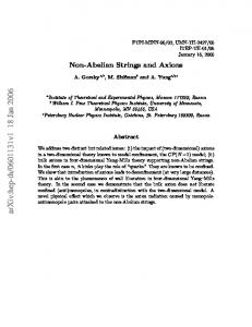
Thus, the vacuum value of ω does not vanish. Looking at Eq. (3.1) one can see that a positive value of ω means that a mass for the fields nl is dynamically generated. To determine the spectrum of the theory one has to expand the effective action Eq. (3.1) around the saddle point and consider field fluctuations in the quadratic approximation. Linear terms vanish. Terms that are cubic and √ higher are suppressed by powers of 1/ N. Two Feynman diagrams in Fig. 1 give rise to the kinetic term for the U(1) gauge field. 8

Figure 1: Feynman diagrams contributing to kinetic term of photon field Gauge invariance requires the answer to be
Πµν = Π(p2 ) p2 gµν − pµ pν .

(3.7)

The meaning of Eq. (3.7) is simple. It represents the kinetic energy of the gauge field written in momentum space. Thus, what was introduced as an auxiliary field becomes a propagating field. Calculation in Appendix B reproduces Witten’s result [14], Π(0) = N/12πΛ2CP , which is interpreted as the inverse of the U(1) charge squared of the nl fields. Massless photon in two dimensions produces the Coulomb potential between two charges at separation R, V (R) =

12πΛ2 R, N

(3.8)

leading to a linear confinement of the n ¯ n pairs. Thus, the spectrum of the theory contains n ¯ n “mesons” rather than free n’s. It is instructive to present an alternative interpretation of this result. In [14] it was shown that nl fields can be interpreted as kinks interpolating between different vacua. The vacuum structure of the CP (N − 1) model was studied in [24]. According to this work the genuine vacuum is unique. There are, however, of the order N quasivacua, which become stable in the limit N → ∞ , since the energy split between the neighboring quasivacua is O(1/N). Thus, one can imagine the n ¯ field interpolating between the true vacuum and the first quasivacuum and the n field returning to the true vacuum as in Fig. 2. The linear confining potential between the kink and antikink is associated with the excess in the quasivacuum energy density compared to that in the genuine vacuum. This two-dimensional confinement of kinks can be interpreted in terms of strings and monopoles of the bulk theory, see [18]. The fine structure of the 9

Figure 2: Configuration of the string with two particles on it. Zero and one represent the true vacuum and the first quasivacuum respectively. CP(N −1) vacua on the non-Abelian string means that N elementary strings are split by quantum effects and have slightly different tensions. Therefore, the monopoles, in addition to the four dimensional confinement, (which ensures that they are attached to the string) acquire a two-dimensional confinement along the string. The monopole and antimonopole connected by a string with larger tension form a mesonic bound state. Consider a monopole-antimonopole pair interpolating between strings 0 and 1, see Fig. 2. The energy of the excited part of the string (labeled as 1) is proportional to the distance as in Eq. (3.8). When it exceeds the mass of two monopoles (which is of order of ΛCP ) then the second monopole-antimonopole pair appear breaking the excited part of the string. This gives an estimate for the typical length of the excited part of the string, R ∼ N/ΛCP . The above condition guarantees that there is enough energy in the “wrong string” to produce a pair of kinks. However, the probability of this process, string breaking, (which can be inferred from the false vacuum decay theory) is proportional to exp(−N), i.e. dies off exponentially at large N.

4

The Coulomb/confinement phase

In order to consider closed non-Abelian strings of length L we compactify the space dimension; in other words, we study CP(N − 1) model (3.1) on a strip of the finite length L with periodic boundary conditions. In Euclidean formulation considering a model at finite length is equivalent to considering the model at finite temperature. The correspondence between the length of the string and the temperature is given by L=β,

(4.1)

where β is the inverse temperature. Thus, the limit of infinite length is the same as the limit of zero temperature. 10

To solve the CP(N − 1) model on a finite strip we use large-N approximation. The CP (N − 1) model at finite temperature in the large-N approximation was solved previously by Affleck [15], see also [16] and [17] for reviews. Although we use a different regularization, our results match those obtained in [15]. There are two important differences, however. The first one is related to the interpretation of the photon mass. In [15] the emergence of the photon mass is interpreted as a phase transition into the deconfinement phase already at L = ∞. We give a different interpretation of the photon mass (see Sec. 4.2); we do not detect any phase transition at L = ∞. We interpret the large L phase (L > 1/ΛCP ) as a Coulomb/confinement phase, much in the same way as at infinite L [14]. The second difference with Ref. [15] is that we find a phase transition at L ∼ 1/ΛCP into a deconfinement phase in the limit N → ∞, see Sec. 5. This is a weak coupling phase. In this phase the global SU(N) is broken and the CP(N − 1) model does not develop a mass gap. The gauge field remains auxiliary and no Coulomb/confining potential is generated. At large but finite N we expect the phase transition to become a rapid crossover. The spontaneous breaking of the global SU(N) symmetry is in a contradiction with the Coleman theorem [23], stating that there can be no massless non-sterile particles in 1 + 1 dimensions. Therefore we expect that the “would be Goldstone” states of the broken phase acquire small masses suppressed in the large-N limit. To solve the CP(N − 1) model we use the mode expansion with the periodic boundary conditions. The open string setup involves the Dirichlet boundary conditions. For example, for open string the expansion (1.1) is modified. It acquires L-independent terms coming from the energy associated with boundaries. We limit ourselves to a closed string in this paper.

4.1

Large-N solution

Our starting point is Eq. (3.1). Integrating out nl fields, one arrives at the same Eq. (3.3) as in the infinite L case. However, now we take into account the gauge holonomy around the compact dimension. Following [15] we choose the gauge A1 = 0 and look for minima of the potential with A0 = const and ω = const. The mode expansion in (3.3) gives for the orientational part of the string energy 11

in (1.3) ( )  2 ∞ Z ∞ 2πk N X dq1 ln q12 + Eorient (L) = + A0 + ω . 2π k=−∞ −∞ L

(4.2)

To calculate (4.2) we follow [26] and use the zeta function regularization. Details of our calculation are presented in Appendix A. Here we give the final result for the string vacuum energy, " # √ ∞ X NLω K1 (kL ω) ω √ Eorient (L) = 1 − ln 2 − 8 cos kLA0 , (4.3) 4π ΛCP kL ω k=1 where K1 is the modified Bessel function of the second kind (also known as the Macdonald function). An important feature of this expression is the appearance of a non-trivial potential for the photon field. We will dwell on this issue in the next subsection. To find the saddle point we extremize the expression (4.3) with respect to ω and A0 , which results in the following equations: √ ∞ √ ∂Eorient 2NL ω X K1 (Lk ω) sin LkA0 = 0 , = (4.4) ∂A0 π k=1 ∞

log

X √ ω K0 (Lk ω) cos LkA0 , = 4 2 ΛCP

(4.5)

k=1

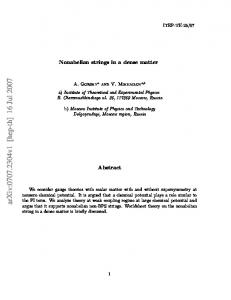
where the logarithmic term in the left-hand side of Eq. (4.5) is the renormalized inverse coupling 1/λ. The logarithmic integral over momentum is regularized in the infrared by ω. Equation (4.4) yields the solution of the form LA0 = π l, where l ∈ Z. However, from the Eq. (4.3) it is clear that the solution with LA0 = 2π l lies lower in energy than the solution with LA0 = (2l − 1)π and is, thus, physical. We take A0 = 0 as a solution of (4.4). Our result for the orientational string energy is shown in Fig. 3, where V˜ = Eorient /L. Equation (4.5) yields a nonvanishing value of ω which we interpret – as in the case of zero temperature – as mass generation for the nl fields. The dependence of the mass on the string length L is shown in Fig. 4 where we put √ ω ≡ m. (4.6) 12

Ž 4ΠV 2.0 1.5 1.0 0.5

2

3

4

5

L

6

-0.5 -1.0

Figure 3: Effective potential (in units of Λ2CP ) as a function of length.

m 1.6 1.5 1.4 1.3 1.2 1.1 1.0

1

2

3

4

5

6

L

Figure 4: Mass (in the units of Λ) of fields nl as a function of L. One can see that the nl field mass increases with decreasing L. In the limit L ≫ 1/ΛCP the modified Bessel functions in (4.3) exhibit exponential fall-off at large L. To determine the leading non-trivial correction to the string energy we can use the “zeroth-order” solution ω ≈ Λ2CP of the equation (4.5) for the vacuum expectation value (VEV) of ω. Clearly this “zeroth-order” solution coincides with the VEV of ω in the infinite volume, see (3.6). For the total string energy we obtain r r   N 2 2 ΛCP −ΛCP L π 1 E(L) = 2πξ + ΛCP L − −N e + · · · . (4.7) 4π 3 L π L In Eq. (4.7) we included the classical string tension 2πξL, its renormalization 13

due to vacuum fluctuations in CP (N − 1) (i.e. (N/4π) Λ2CP L), and the contribution of the translational modes which give the standard L¨ uscher term. This result was quoted in Sec. 1, see Eq. (1.5). We see that the quantum fluctuations of the orientational moduli contribute both to the renormalization of the string tension (the linear in L term in (4.7)) and to the function f (ΛCP L) in (1.3). As was expected, in the theory with a mass gap the contribution of orientational moduli to the L-dependent part of the string energy is exponentially suppressed at large L. Let us note, that the case of an open non-Abelian string was previously considered in [27]. The results of [27] show the presence of long range 1/L effects coming from the orientational sector even at large L where the theory has a mass gap. We disagree with these results and believe that orientational long range forces in the large-L phase are spurious and are associated with the boundary energy somehow induced [27] by the Dirichlet boundary conditions rather than with the string itself.

4.2

The photon mass

The A0 -dependence in the potential (4.3) ensures that the gauge field acquires a mass [15]. It is quite natural to expect that the photon becomes massive at non-zero temperature. Physically this means the Debye screening. Expanding (4.3) at large L we can write down an effective action for the U(1) gauge field, ( ) r r Z 1 2 2 ΛCP −ΛCP L Sgauge = d2 x Fkl − N e cos A0 L + · · · . (4.8) 2 4e π L3 The kinetic term for the gauge field at non-zero temperature is calculated in Appendix B. To calculate the photon mass to the leading order in exp (−ΛCP L) we need the expression for the gauge coupling e2 in the limit L → ∞, namely, N 1 ≈ , (4.9) 2 e 12πΛ2CP see Sec. 3. Expanding (4.8) to the quadratic order in A0 we arrive at p m2A ≈ 12Λ2CP 2πΛCP L e−ΛCP L . (4.10) for the photon mass. Note, that the non-zero photon mass at finite temperature does not break gauge invariance since Lorentz symmetry is explicitly broken, see [15]. 14

The photon becoming massive was the reason for the claim [15] that at non-zero temperature the CP(N − 1) model is in the deconfinement phase. We give a different interpretation for this effect. We treat the quasivacua as the strings of different tension. Kinks and antikinks interpolate between true vacuum and the first quasivacuum. The Debye screening due to a finite photon mass now can be interpreted as a breaking of the confining string between kink and antikink in the thermal medium (through picking up a kink-antikink pair from the thermal bath). Note, that unlike pair-production from the vacuum, this process is not suppressed as exp(−N). The kink-antikink potential has the form V (R) = e2 R e−mA R ,

(4.11)

where R is the kink-antikink separation. It is still linear at small R, while the exponential suppression at large R can be understood as a breaking of the confining string due to creation of a kink-antikink pair from the thermal bath. Therefore, we still interpret the large L phase as a Coulomb/confinement phase. A similar question can be addressed in QCD. Do we have confinement of quarks in QCD? We believe that the answer is positive. However, the confining string can be broken by quark-antiquark production. We suggest a similar interpretation for the CP(N − 1) model at non-zero temperature. If L is very large (very low temperatures) the thermal string breaking can be ignored, however once L reduces below log N/ΛCP the thermal breaking becomes operative.

4.3

Small length limit

As was already mentioned, we will show in the next section that once L decreases below 1/ΛCP our CP(N − 1) model undergoes a phase transition into the deconfinement phase. To prove this we calculate the vacuum energy in the deconfinement phase in the next section and show that it lies below that in the Coulomb/confinement phase. In order to make this comparison we will examine Eqs. (4.3) and (4.5) in the low-L limit. These expressions determine the vacuum energy and the ω expectation value in the Coulomb/confinement phase.

15

Assuming that L2 ω ≪ 1 we can use the following approximation for the sum of the modified Bessel functions (see Eq. (8.526) in [21]) ∞ X n=1

K0 (ny) ≈

π 1 y γ + ln + + O(y 2) , 2y 2 4π 2

where γ ≈ 0.577 is the Euler-Mascheroni constant. from (4.5)  √ √ π ω 1 L ω √ + ln =2 + ln ΛCP 4π 2L ω 2 or approximately

1

(4.12)

Consequently, we get  γ , 2

(4.13)

π √ . (4.14) ΛCP L L ω Now the logarithmic integral which determines the renormalized √ inverse coupling 1/λ is regularized in the infrared by 1/L rather than by ω (which is the case in the large-L limit). This gives us the ω expectation value, ln

√

ω=

=

1 π +··· . L ln (1/ΛCP L)

(4.15)

Equation (4.15) justifies our approximation L2 ω ≪ 1 at L ≪ 1/ΛCP . Note also that at L ≪ 1/ΛCP the coupling constant is small – it is frozen at the scale 1/L (the logarithm in the left-hand side of (4.14) is large), so the theory is at weak coupling. To find the orientational energy in this limit we need to find an approximate expression for the sum of the modified Bessel functions that appears in (4.3), √ ∞ √ 2L ω X K1 (kL ω) SE = . (4.16) Lπ k=1 k

Derivative of the modified Bessel functions satisfies the following relation (see Eq. (9.6.28) in [20]): K1′ (x) = −K0 (x) −

K1 (x) . x

(4.17)

Let us introduce a notation, S1 (x) =

∞ X K1 (kx) k=1

16

k

.

(4.18)

Then ′

(xS1 (x)) = −x

∞ X

K0 (kx)

k=1

(4.12)

≈

−

π x x xγ − ln − + O(x3 ) . 2 2 4π 2

(4.19)

Integrating this expression one finds xS1 (x) ≈ −

xπ x2 x x2 − ln − (2γ − 1) + const + O(x4 ) 2 4 4π 8

(4.20)

The behavior of the modified Bessel function at small values of the argument is given by (see Eq. (9.6.9) in [20]) K1 (x) ∼

1 . x

(4.21)

Thus, the sum S1 (x) can be approximated as follows: ∞ X 1 π2 S1 (x) ≈ = . xk 2 6x k=1

(4.22)

Hence the constant appears to be π 2 /6. Now we are ready to present the approximate expression we seek for, √ √ √ 2 √ π Lω L ω Lω SE = L ωS1 (L ω) ≈ − ω− ln − (2γ − 1) . (4.23) Lπ 3L 2π 4π 4π With this approximation we arrive at the orientational energy Eorient (L) = −

√ π N 1 N +N ω− ωL ln +··· 3 L 2π ΛCP L

(4.24)

Substituting here the VEV of ω, see (4.15), we get Eorient (L) = −

π N π N 1 + +··· . 3 L 2 L ln (1/ΛCP L)

(4.25)

The first term here is the L¨ uscher term proportional to the number of orientational degrees of freedom 2(N −1) ≈ 2N (in the large N limit). It gets corrected by an infinite series of powers of inverse logarithms ln (1/ΛCP L), if we naively extend the Coulomb/confinement phase into the region of small L. We will show in the next section that in fact the theory undergoes a phase transition into a different phase, with a lower energy. 17

5

Deconfinement phase

Classically CP(N −1) model has 2(N −1) massless states which can be viewed as Goldstone states of the broken SU(N) symmetry. Indeed, classically the vector nl satisfies a fixed length condition, |n|2 = r, see (3.1). Thus classically nl acquires a VEV breaking SU(N) symmetry. However, as was shown above, in the strong coupling large L domain the spontaneous symmetry breaking does not occur, in much the same way as in the infinite-L limit, see [14]. At strong coupling the vector nl is smeared all over the vacuum manifold due to strong quantum fluctuations. The theory has a mass gap, moreover the number of the massive n-fields becomes 2N. Effectively the classical constraint |n|2 = r is lifted, see [14]. At small L the theory enters a weak coupling regime so we expect occurrence of the classical picture in the limit N → ∞. To study this possibility we assume that one component of the field nl , say n0 ≡ n can develop a VEV. Then we integrate over all other components of nl (l=1,2,...) keeping the fields n and ω as a background. Note, that a similar method was used in [28] for studying phase transitions in the CP(N − 1) model with twisted masses. Now, instead of (4.24), we get Eorient (L) = ωL |n|2 −

π N N 1 − ωL ln +··· , 3 L 2π ΛCP L

(5.1)

where the ellipses stand for higher terms in L2 ω. Note, that here we drop the contribution associated with the integration over the constant n (the second term in (4.24)) because we introduce n0 as a constant background field (in other words, we drop the term with k = 0 in (4.2)). Minimizing over ω and n we arrive at the equations |n|2 =

1 N ln + ..., 2π ΛCP L

(5.2)

ωn = 0. The solution to these equations with nonzero n0 read |n|2 =

1 N ln , 2π ΛCP L

18

ω = 0.

(5.3)

We see that the mass gap ω is not generated. Substituting this in (5.1) we get that the orientational energy reduces just to the L¨ uscher term, namely Eorient (L) = −

π N . 3 L

(5.4)

This energy is lower than the one in (4.25). Therefore, we conclude that at L ∼ 1/ΛCP the theory undergoes a phase transition into the phase with the broken SU(N) symmetry. This ensures the presence of 2(N − 1) Goldstone states nl , l = 1, ...(N − 1). The photon remains an auxiliary field, no kinetic term is generated for it. As a result, there is no Coulomb/confining linear rising potential between the n-states. The phase with the broken SU(N) is a deconfinemet phase. Since |nl | is positively defined Eq. (5.3) shows that this phase appears at L < 1/ΛCP . The results of numerical calculations are in agreement with our conclusions. The relation between orientational energies in both phases is shown in Fig. (5). One can see that the L¨ uscher term energy is lower and is thus physical.

Ž V 0

0.2

0.4

0.6

0.8

1.0

L

-50

-100

-150

Figure 5: Comparison of orientational energies in both phases. The L¨uscher term always lies lower. We set ΛCP = 1. The phase with the broken symmetry in two dimensions can occur only in the limit N → ∞. As was already explained, if N is large but finite this would contradict the Coleman theorem [23]. Therefore, we expect that at large but finite N the phase transition becomes a rapid crossover. In 19

particular, we expect that the nl fields are not strictly massless. They have small masses suppressed by 1/N. To conclude this section let us note that the CP (N − 1) model compactified on a cylinder with the so-called twisted boundary conditions was studied in [29]. No phase transition was found; moreover, it was shown that the theory has a mass gap which shows no L-dependence and is determined entirely by ΛCP . We believe that our results are not in contradiction with those obtained in [29], because at finite L the boundary conditions matter: they can be crucial. In particular, the twisted boundary conditions can be viewed as a gauging of the global SU(N) group with a constant gauge potential. Then the global SU(N) is explicitly broken. This model should be considered as distinct as compared to the CP(N − 1) model with the periodic boundary conditions studied in this paper.

6

Supersymmetric CP(N − 1) model with no compactification

Non-Abelian strings were first found in N = 2 supersymmetric QCD with the U(N) gauge group and Nf = N quark hypermultiplets [5, 6, 7, 8], see [9, 10, 11, 12] for reviews. In much the same way as for non-supersymmetric case the internal dynamics of orientational zero modes of non-Abelian string is described by two-dimensional CP(N −1) model living on the string world-sheet. The string solution is 1/2-BPS saturated; therefore the two-dimensional model under consideration is N = (2, 2) supersymmetric. In this section we briefly review the large-N solution of N = (2, 2) CP(N − 1) model in infinite space [14]. In the next section we will present the large-N solution of the model on a strip of a finite length L (cylindrical compactification). The bosoinc part of the action of the CP(N − 1) model is given by Z h 1 1 1 Sbos = d2 x |∇i nl |2 + 2 Fij2 + 2 |∂i σ|2 + 2 D 2 4e e 2e i + 2|σ|2|nl |2 + iD(|nl |2 − r0 ) , (6.1)

where the covariant derivative is defined as ∇i = ∂i − iAi and σ is a complex scalar field, the scalar superpartner of Ai . Moreover, r0 is the bare coupling constant. In the limit e2 → ∞ the gauge field Ai and σ become auxiliary 20

fields. D stands for the D component of the gauge multiplet. The factor i is due to the passage to the Euclidean notation. The fermionic part of the action takes the form Z h Sf erm = d2 x ξ¯lR i(∇0 − i∇3 )ξRl + ξ¯lL i(∇0 + i∇3 )ξLl 1¯ 1¯ λR i(∇0 − i∇3 )λR + 2 λ L i(∇0 + i∇3 )λL 2 e e √ i √ + i 2σ ξ¯lR ξLl + i 2¯ nl (λR ξLl − λL ξRl ) + H.c. ,

+

(6.2)

l where the fields ξL,R are the fermion superpartners of nl and λL,R belong to the gauge multiplet. In the limit e2 → ∞ they enforce the following constraints: n ¯ l ξLl = 0 , n ¯ l ξRl = 0 . (6.3)

The field σ is auxiliary and can be eliminated, namely, σ = −√

6.1

i ¯ l ξlL ξR . 2r0

(6.4)

Large-N solution

The N = (2, 2) supersymmetric CP(N − 1) model was solved in the largeN limit by Witten [14], see also [22]. In this section we briefly review this solution. Since both fields nl and ξ l appear quadratically we can integrate them out. This produces two determinants,

(6.5) det−N −∂i2 + iD + 2|σ|2 detN −∂i2 + 2|σ|2

The first determinant comes from the boson nl fields, while the second comes from the fermion ξ l fields. Note that if D = 0 the two contributions obviously cancel each other, and supersymmetry is unbroken. As before, the non-zero values of iD + 2|σ|2 and 2|σ|2 can be interpreted as non-zero values of the mass of nl and ξ l fields, and we put Ak = 0. The final expression for the effective potential is given by (see, for example, [22])   Z iD + 2|σ|2 2|σ|2 2 N 2 2 Veff = d x −(iD + 2|σ| ) ln + iD + 2|σ| ln 2 , (6.6) 4π Λ2CP ΛCP 21

where the logarithmic ultraviolet divergence of the coupling constant is traded for the scale ΛCP . To find a saddle point we minimize the potential with respect to D and σ, which yields the following set of equations: ln

iD + 2|σ|2 = 0, Λ2CP

ln

iD + 2|σ|2 = 0, 2|σ|2

(6.7)

The solution to these equations is D = 0, which shows that supersymmetry is not broken. The VEV of σ is √ 2πk 2σ = ΛCP e N i , k = 0, ..., (N − 1).

(6.8)

(6.9)

We see that σ develops a VEV giving masses to the nl fields and their fermion superpartners ξ l . The phase factor in the right-hand side of (6.9) does not follow from (6.7). It comes from the broken chiral U(1) symmetry. The axial anomaly breaks it down to Z2N . The field σ has the chiral charge 2. This explains the phase factor in (6.9). Once |σ| has a nonzero VEV the anomalous symmetry breaking ensures that the theory has N vacuum states. Clearly this fine structure cannot be seen in the large N approximation since the phase factor is a 1/N effect. In full accord with the Witten index, the solution above has N vacua, each with the vanishing energy. Consider now the vector multiplet. In much the same way as in the non-supersymmetric case, photon becomes a propagating field. To find the renormalized gauge coupling one needs to evaluate two Feynman diagrams shown in the Fig.6. Details of the appropriate calculation are given in Appendix C. The result is 1 N 1 = . (6.10) 2 e 4π Λ2CP Through the coupling to the Im σ (due to the chiral anomaly) now the photon acquires a mass. Moreover, the fermion fields λL,R also become propagating, with the same mass as that of the photon, as required by supersymmetry. The masses of the fields of the vector multiplet are as follows 22

Figure 6: Feynman diagrams contributing to the kinetic term of the photon [14, 22]: mph = mλL,R = mRe σ = mIm σ = 2ΛCP .

(6.11)

Since the photon became massive there is no linear rising Coulomb potential between the charged states. There is no confinement in supersymmetric CP(N − 1) model even in the infinite volume limit. It has N degenerate vacua which are interpreted as N degenerate elementary non-Abelian strings in the four-dimensional bulk theory. In contrast to the non-supersymmetric case, the confined monopoles of the bulk theory, which are seen as kinks interpolating between the CP(N − 1) vacua, are free to move along the string, see [11] for further details.

7

Supersymmetric CP(N − 1) on a cylinder

Now we compactify one space dimension and impose periodic boundary conditions, both for bosons and fermions, in order to preserve N = (2, 2) supersymmetry. We stress that this compactification cannot be considered as thermal. Non-zero temperature requires anti-periodic boundary conditions for fermions, which would break supersymmetry explicitly. The large-N method in the case of N = (2, 2) CP(N − 1) model works similar to that in the non-supersymmetric case. We compactify now the spatial coordinate x1 and start from a slightly modified expression for the determinants in Eq. (6.5). Choosing the A0 = 0 gauge and assuming that A1 is non-zero we write

det−N −∂02 − (∂1 − iA1 )2 + m2b detN −∂02 − (∂1 − iA1 )2 + m2f , (7.1)

where we introduced the following notation: m2b = iD + 2|σ|2, 23

m2f = 2|σ|2 .

(7.2)

The evaluation of each of the determinants is no different from that in the non-supersymmetric case. Again we use the zeta-function method. Using expressions in Appendix C we can derive the effective potential, E =

LN h iD + 2|σ|2 2|σ|2 2 − (iD + 2|σ|2 ) ln + iD + 2|σ| ln 4π Λ2CP Λ2CP

−

8m2b

+

8m2f

∞ X K1 (Lmb k) k=1

Lmb k

∞ X K1 (Lmf k) k=1

Lmf k

cos (LA1 k) i

cos (LA1 k) ,

(7.3)

Here the first line is just the effective potential at L = ∞, while the second and third lines are the finite-L corrections due to bosons and fermions, respectively. To find a stationary point we vary the above expression with respect to A1 , D and σ. The resulting equations are as follows: mb

∞ X k=1

K1 (Lmb k) sin (LA1 k) − mf

∞ X

K1 (Lmf k) sin (LA1 k) = 0 ,

k=1

# ∞ ∞ X X m2b K0 (Lmf k) cos (LA1 k) = 0 , K0 (Lmb k) cos (LA1 k) − 4 2σ − ln 2 + 4 mf "

k=1

k=1

∞

X m2b − ln 2 + 4 K0 (Lmb k) cos (LA1 k) = 0 . ΛCP

(7.4)

k=1

Calculation of the gauge coupling constant at finite L is also modified (see Appendix C). As a result, we arrive at ∞ 1 1 L X K1 (Lmb k)k , = + Ne2 4πm2b 2πmb

(7.5)

k=1

which reduces to 1/4πΛ2CP in the limit L → ∞. Consider now the large L limit, L ≫ 1/ΛCP . Assuming that mb ∼ mf ∼ ΛCP (we confirm this below) we expand the string energy (7.3) keeping the

24

first exponentially small term   m2f m2f LN 2 2 E = −mb ln 2 + iD + mf ln 2 4π ΛCP ΛCP r r r  2 mb −mb L mf −mf L cos A1 L + · · · . e − e − N π L L √ Taking derivatives with respect to D, 2¯ σ and A1 we obtain

(7.6)

2

m2 1 exp (−mb L) N √ − log 2 b + N √ cos A1 L + · · · = 0, 4π ΛCP mb L 2π " ( # ) √ m2f 1 exp (−mb L) exp (−mf L) N √ log 2 + N √ 2σ cos A1 L + · · · = 0, − p 4π mb mb L mf L 2π (

exp (−mb L) exp (−mf L) √ − p mb L mf L

)

sin A1 L + · · · = 0 ,

(7.7)

where the ellipses denote next-to-leading corrections in 1/Lmb and 1/Lmf . The solution of these equations is as follows. The second and third equations are satisfied at D = 0, (7.8) which shows that supersymmetry is not broken. A1 remains undetermined. With D = 0 the first equation determines the σ expectation value, namely, √
N 2|σ|2 1 exp − 2|σ|L q√ log 2 = N √ cos A1 L + · · · . (7.9) 4π ΛCP 2π 2|σ|L

This equation seems to present a puzzle. It shows that the VEV of σ depends on the parameter A1 , which is arbitrary. If this were the case the theory would have a branch of vacua parametrized by the Polyakov line R

e

dx1 A1

= eiA1 L ,

(7.10)

which measures the holonomy around the compact dimension. More exactly, the theory would have N branches of vacua, because Z2N symmetry ensures 25

that the overall phase of σ takes N values 2πk/N, k = 0, ..., (N − 1). This would contradict the Witten index argument which ensures that the number of vacua is equal to N for N = (2, 2) supersymmetric CP(N − 1) model. The resolutionR of this puzzle is that we should quantize the phase variable A1 L (note that dx1 A1 depends only on time) as a function of the noncompact time. In the emerging quantum mechanics the phase A1 L is not fixed; instead, it is smeared all over the circle (in the ground state). As a result, the cos (A1 L) in (7.9) is averaged to zero and the σ VEVs are given by √ 2πk k = 0, ..., (N − 1). (7.11) 2σ = ΛCP e N i ,

This is exactly the same result as for L = ∞. All cosine functions of A1 L in the last equation in (7.4) are averaged to zero, therefore the result in (7.11) is exact and does not depend on L. This result also can be understood by studying the exact twisted superpotential of N = (2, 2) CP(N − 1) model. In the infinite volume it is given by [30, 31, 32] ( ) √ N √ 2σ √ 2σ log W (σ) = − 2σ . (7.12) 4π ΛCP

This superpotential has correct transformation properties with respect to the chiral U(1) symmetry. Namely, integrated over half of the superspace it is invariant under chiral symmetry up to a term which precisely reproduces the chiral anomaly. Now at finite length this superpotential in principle could have corrections proportional to powers of   √ (7.13) exp − 2σL .

However these corrections would spoil the transformation properties of the superpotential with respect to the chiral symmetry. Therefore they are forbidden. As a result at finite L the exact superpotential of the theory is still given by (7.12). Critical points of this superpotential are given by (7.11) and do not depend on L. This matches our result obtained from large-N approximation. In particular, at small L the theory is at weak coupling and can be studied in the quasiclassical approximation. As we already mentioned CP(N − 1) model compactified on a cylinder with twisted boundary conditions was studied in [29]. It is shown in [29] that the mass gap at weak coupling is produced by fractional instantons and does not depend on L both in supersymmetric 26

and non-supersymmetric cases. For our case (periodic boundary conditions) the mass gap shows L-dependence in non-supersymmetric case, while in the supersymmetric case it is L-independent. The quasiclassical origin of this behavior needs to be understood in the weak coupling domain of small L. This is left to a future work. To conclude, in N = (2, 2) supersymmetric CP(N − 1) model we have a single phase with the unbroken supersymmetry and N vacua. Each vacuum has vanishing energy and parametrized by the VEV of σ in Eq. (7.11). Unlike non-supersymmetric problem, this VEV is independent of L.

8

The photon mass

In this section we outline the photon mass calculation. The effective action for the gauge field can be written as [22]   Z 1 2 N σ ∗ 2 Sgauge = d x , F − log F 4e2 kl 4π σ ¯

(8.1)

where the photon mixing with σ is due to the chiral anomaly and 1 (8.2) F ∗ = ǫij F ij 2 is the dual gauge field strength. In the case of infinitely long string the the gauge coupling and the photon mass were found [22], 1 N 1 = , e2 4π Λ2CP

(8.3)

mph = 2ΛCP ,

(8.4)

and respectively. In Sec. 7 we derived the expression for the gauge coupling in the case of finite length, see (7.5). The corresponding expression for the photon mass in the limit of ΛCP L ≫ 1 is   p (8.5) m2ph ≈ (2ΛCP )2 1 − 2πΛCP L e−ΛCP L

where we used the asymptotic expansion of the modified Bessel functions (see Eq. (9.7.2) in [20]), r π −x e . (8.6) K1 (x) ∼ 2x 27

Since K0′ (x) = −K1 (x) we can also determine the photon mass in the opposite limit of ΛCP L ≪ 1, !′ ∞ ∞ X X 1 π K1 (kx)k = − K0 (kx) ≈ 2 − , 2x 2x k=1 k=1 m2ph ≈

9

ΛCP L (2ΛCP )2 ≪ (2ΛCP )2 . π

(8.7)

Conclusions

We studied two-dimensional CP(N − 1) model (both nonsupersymmetric and N = (2, 2)) compactified on a cylinder with circumference L (periodic boundary conditions). We found the large-N solution for any value of L and discussed in detail the large-L and small-L limits. A drastic difference is detected in passing from the nonsupersymmetric to N = (2, 2) supersymmetric case. In the former case in the large-N limit we observe a phase transition at L ∼ Λ−1 CP (which is expected to become a rapid crossover at finite N). At large L the CP(N −1) model develops a mass gap and is in the Coulomb/confinement phase, with exponentially suppressed finite-L effects. At small L it is in the deconfinement phase; the orientational modes contribute to the L¨ usher term. The latter becomes dependent on the rank of the bulk gauge group. In the supersymmetric CP(N − 1) model we have a different picture. Our large-N solution exhibits a single phase independently of the value of LΛCP . For any value of this parameter a mass gap develops and supersymmetry remains unbroken. So does the SU(N) symmetry of the target space (i.e. it is restored). The mass gap turns out to be independent of the string length. The L¨ uscher term is absent due to supersymmetry.

Acknowledgments We are grateful to A. Vainshtein for illuminating insights. A.Y. is also grate¨ ful to M. Anber, T. Sulejmanpasic and M. Unsal for very useful discussions. This work is supported in part by DOE grant de-sc0011842. The work of A.Y. was supported by William I. Fine Theoretical Physics Institute of the University of Minnesota, by Russian Foundation for Basic Research under 28

Grant No. 13-02-00042a and by Russian State Grant for Scientific Schools RSGSS-657512010.2. The work of A.Y. was supported by Russian Scientific Foundation under Grant No. 14-22-00281.

Appendix A: Calculation of Zeta function We define the zeta function of an operator Ω as follows: ζ(s) = T r Ω−s .

(A.1)

The operator of interest is given in Eq. (3.3), Ω = −(∂k − iAk )2 + m2 ,

(A.2)

where instead of ω we write m2 . In the A1 = 0 gauge the expression for the zeta function takes the form !−s  2 ∞ Z ∞ X ˆ 2πk T ζ(s) = dq1 q12 + + A0 + m2 . (A.3) 2π k=−∞ −∞ L Gauge invariance requires invariance under transformation A0 → A0 +2πk0 /L, where k0 is integer. This is manifest in (A.3) since the shift can be absorbed in the sum. We always can look for a solution for A0 in the interval |A0 | < π/L, say A0 = 0. To evaluate the expression in (A.3) we will need the following identities Z ∞ Γ(Z) = dt tz−1 e−t , (A.4) 0

Z

∞ 0

1 dx(x2 )(α−1)/2 (x2 + A2 )β−1 = (A2 )β−1+α/2 B(α/2, 1 − β − α/2) , 2

B(x, y) =

Γ(x)Γ(y) . Γ(x + y)

(A.5)

The definition of the modified Bessel functions of second kind is Z ∞   a ν/2  √   a Kν 2 ab . dx xν−1 exp − − bx = 2 x b 0 29

(A.6)

The definition of the theta function (see Chapter 21 of [25]) is Θ3 (x, τ ) =

∞ X

k2

2πix

q e

=1+2

k=−∞

∞ X

2

q k cos 2kx ,

q = eπiτ ,

(A.7)

k=1

Its Jacobi transformation is Θ3 (x, τ ) = (−iτ )

−1/2

exp



x2 iπτ



Θ3 (x/τ, −1/τ ) .

(A.8)

The evaluation of the zeta function, Eq. (A.3), proceeds as follows: ζ(s)

=

" #1/2−s 2 ∞ Tˆ Γ( 12 )Γ(s − 21 ) X 2πk + A0 + m2 2π Γ(s) L k=−∞

=

 1−2s X ∞ Tˆ Γ( 12 )Γ(s − 21 ) 2π 2π Γ(s) L

(A.5)

k=−∞

=

 1−2s 1 Tˆ Γ( 12 )Γ(s − 21 ) 2π 2π Γ(s) L Γ(z)

×

Z

(A.4)

(A.7)

=

× (A.8),(A.7)

=

(A.6)

=

∞ z−1 −tα2

dt t

e

0

∞ X

e−k

" #1/2−s 2 LA0 k+ + ǫ2 2π

2 t−kβ 2 t

k=−∞

 1−2s 1 Tˆ Γ( 12 )Γ(s − 21 ) 2π 2π Γ(s) L Γ(z)   2 Z ∞ iβ t it z−1 −tα2 dt t e Θ3 , 2 π 0 F

√

π Γ(z) √

π F Γ(z)

Z

∞



1 G2

2 +β 4 t/4

dt tz−3/2 e−tα

0

1+2

∞ X k=1

z− 21

30

2 2 − k tπ

e

cos πkβ 2

!

∞ X 1 1 Γ(z − ) + 4 (πkG)z− 2 Kz− 1 (2πkG) cos πkβ 2 2 2 k=1

× (A.6)

=

 Tˆ L 1 1 2s−2 4π m s−1 ∞

4 X Γ(s)

+

!

k=1



Lmk 2

s−1

#

Ks−1(Lmk) cos LA0 k ,

(A.9)

where we introduced intermediate notations Lm , ǫ= 2π

1 z =s− , 2

 1−2s Tˆ Γ( 21 )Γ(s − 12 ) 2π F = , 2π Γ(s) L

(A.10)

and 2

α =



LA0 2π

2

+



Lm 2π

2

,

β2 =

LA0 , π

G2 = α2 − β 4 /4 .

(A.11)

To find the derivative of the zeta function we will make use of the following properties of Euler’s Γ function: Γ(z + 1) = zΓ(z) ,

Γ(0) = ∞ .

(A.12)

The derivative is evaluated as follows: " ˆ TL 1 2 ln m 1 − 2s−2 ζ ′(s) = − 2s−2 2 4π m (s − 1) m (s − 1) # s−1 ∞  4Γ′ (s) X Lmk Ks−1 (Lmk) cos LA0 k − 2 2s−2 Γ (s)m 2 n=1

s=0

"

∞ X Tˆ Lm2 K1 (kLm) 2 = −1 + ln m + 8 cos LA0 k 4π kLm k=1

#

(A.13)

Following [26] we can write the generating functional, 1 1 ln Z = ζ ′(0) + ln µ2 ζ(0) , 2 2 31

(A.14)

where a normalization constant µ has dimension of mass. Renormalizability requires µ = Muv . Thus, in terms of the zeta function and its derivative the expression for the effective potential becomes V =−


N N ′ M2 2 ζ (0) + ζ(0) ln Muv Lm2 ln uv . − 4π Λ2 Tˆ

(A.15)

Substituting the expressions for the zeta function and its derivative we obtain " # √ ∞ X K1 (kL ω) ω NLω √ 1 − ln 2 − 8 V = cos kLA0 , (A.16) 4π ΛCP kL ω k=1 where we replaced m2 by ω.

Appendix B: Kinetic term in case of bosonic theory To find the U(1) charge of the nl fields one has to consider only the second diagram in Fig. (1). The first diagram is needed only for renormalization. The relevant part of the action written in the Minkowski spacetime takes the form Z   M iSB = i d2 x ∇µ n ¯ l ∇µ nl − m2 |n|2 = i

Z

i h ← → l µ 2 2 µ 2 2 d x ∂µ n ¯ l ∂ nl − m |n| + iA (¯ nl ∂ µ n ) + A |n| , (B.1) 2

← → → − ← − where ∂ µ = ∂ µ − ∂ µ . We then pass to Euclidean space, t = −iτ ,

A0 = iAˆ0 ,

Ai = Aˆi .

The action in Euclidean space is Z i h ← → E SB = d2 xˆ ∂k n ¯ l ∂k nl + m2 |n|2 + iAˆk (¯ nl ∂ k nl ) + Aˆ2 |n|2 . 32

(B.2)

Figure 7: Feynman rules: vertex and the propagator of nl field. Now we can determine the Feynman rules. The results are shown in Fig. (7). Thus for the kinetic term (in the case of an infinitely long string) one can write Z (pi + 2qi )(pj + 2qj ) d2 q . (B.3) Πij = N (2π)2 (m2 + q 2 )(m2 + (p + q)2 )

Introducing the Feynman parameter to combine the denominators Z 1 1 1 = , dx α(α + β) (xβ + α)2 0 and substituting l = q + px in Eq. (B.3) we arrive at Z 2 d l dx [pi pj (1 − 2x)2 − 2x(pi lj + pj li ) + 4li lj ] Πij = N . (2π)2 (l2 + m2 + p2 x(1 − x))2

(B.4)

(B.5)

Terms linear in l vanish. To find the U(1) charge we only need to consider the pi pj structure. Thus, the expression for the charge is 1 = Ne2

Z

d2 l dx (1 − 2x)2 = (2π)2 (l2 + m2 + p2 x(1 − x))2

Z

1 0

dx (1 − 2x)2 . (B.6) 4π m2 + p2 x(1 − x)

Expanding the last expression to the zeroth power in p one finally finds Z 1 1 dx 1 = (1 − 2x)2 = . (B.7) 2 2 Ne 12πm2 0 4πm 33

The case of the finite length string is considered along similar lines. We recall (see [15]) that the limit pµ → 0 is understood as first putting p0 = 0 and then letting p1 go continuously to zero. As a result, only Π00 6= 0. Using the Feynman rules one can derive the following expression: Π00

∞ Z dq N X 4ωk2 = , L k=−∞ 2π (m2 + q 2 + ωk2 )(m2 + (p + q)2 + ωk2 )

(B.8)

where we defined ωk = 2πk/L. Introducing again the Feynman parameter and making the same substitution one arrives at Π00

Z ∞ X Nωk2 1 dx = . 2 2 + ω + p2 x(1 − x))3/2 L (m 0 k k=−∞

(B.9)

We expand this expression and keep only the leading power in p. Then the expression for the charge becomes # " ∞ ∞ X X 1 1 (m2 + ωk2 )−5/2 (m2 + ωk2)−3/2 − m2 = Ne2 4L k=−∞ k=−∞ L2 = 32π 3

"

∞ X

2

2 −3/2

(k + α )

k=−∞

−α

2

∞ X

2

2 −5/2

(k + α )

k=−∞

#

, (B.10)

where α = Lm/2π. We deal with these sums as follows: S1 (z, α)

≡ (A.7)

=

(A.8)

=

(A.6)

=

∞ X

2

2 −z (A.4)

(k + α )

=

k=−∞

1 Γ(z)

Z

∞ z−1 −tα2

dt t 0

e

∞ X

e−k

2t

k=−∞

∞ 1 2 dt tz−1e−tα Θ3 (0, it/π) Γ(z) 0 √ Z ∞ π 2 dt tz−1e−tα Θ3 (0, −π/it) Γ(z) 0 # z− 12 √ " ∞  X kπ π Γ(z − 12 ) Kz− 1 (2kπα) . (B.11) +4 2 Γ(z) α2z−1 α

Z

k=1

34

Thus the expression for the charge can be written as  3   1 L 1 2 S (3/2, α) − α S (5/2, α) = 1 1 Ne2 4L 2π ∞

∞

L2 X L X 1 K (kLm) k − K2 (kLm) k 2 . (B.12) + = 1 2 12πm 2πm k=1 6π k=1

In the limit Lm ≫ 1 the contributions from the modified Bessel functions are exponentially small and thus the expression for the charge reduces to that for the infinitely long string.

Appendix C: Kinetic term in the supersymmetric case In Appendix B we calculated the first diagram (the boson part) in Fig. 6. Now we will calculate the second diagram (the fermion part). The relevant part of the fermion action in the Minkowski spacetime is (   Z 5 √ 1 − γ M 2 µ iSF = i d x ξ¯ iγ ∇µ ξ − i 2σ ξ¯ ξ 2  )  5 √ ∗ 1 + γ ξ , (C.1) + i 2σ ξ¯ 2 where ∇µ = ∂µ − iAµ is the covariant derivative, and the γ matrices are defined as       0 −i 0 i 1 0 0 1 5 γ = , γ = , γ = . i 0 i 0 0 −1 We pass to Euclidean space, t = −iτ ,

A0 = iAˆ0 ,

Ai = Aˆi ,

γˆ 0 = γ 0 ,

γˆ 1 = −iγ 1 ,

γˆ 5 = γ 5 ,

and, since in Euclidean formulation ξ and ξ¯ are independent, we define ξˆ = ξ ,

ξˆ¯ = iξ¯ . 35

Thus, the action in Euclidean space can be presented as follows: " Z S E = − d2 xˆ ξˆ¯ iˆ γ k ∂ˆk ξˆ + ξˆ¯ γˆ k Aˆk ξˆ F

−

√

1 − γˆ 5 2σ ξˆ¯ 2 



ξˆ +

√

1 + γˆ 5 2σ ∗ ξˆ¯ 2 

 # ξˆ .

(C.2)

Examining this expression in components one can find that it matches that of (6.2). Since from now on all calculations will be carried out in Euclidean space we will drop the caret notation. Using (C.2) we find the Feynman rules that are shown in Fig. (8), where we introduced a notation σ = a + ib and

Figure 8: Feynman rules: vertex and the propagator of ξ l field. the mass is m2 = 2a2 + 2b2 . We begin from the case of the infinitely long string. The fermion contribution to the kinetic term is Z d2 q 1 ij Π = − 2 2 2 (2π) (q + m )[(p + q)2 + m2 ] i h √ √ √ √ × Tr γ i (/q + i 2b + 2aγ 5 )γ j (p/ + /q + i 2b + 2aγ 5 ) . (C.3)

The Clifford algebra is, as usual,

{γ i γ j } = 2δ ij . 36

(C.4)

As a result, the trace identities for the γ matrices become Tr(γ i γ j ) = 2δ ij , Tr(γ i γ j γ k γ l ) = 2δ ij δ kl − 2δ ik δ jl + 2δ il δ jk ,

Tr(odd number of γ’s) = 0 .

(C.5)

Thus, the expression for the kinetic term takes the form Z d2 q Tr[γ i /qγ j (p/ + /q) − m2 γ i γ j ] ij Π = − (2π)2 (q 2 + m2 )[(p + q)2 + m2 ] Z d2 q 1 = − (2π)2 (q 2 + m2 )[(p + q)2 + m2 ] ˙ + q)δ ij − 2m2 δ ij ] . × [2q i (p + q)j + 2q j (p + q)i − 2q (p

(C.6)

Notice, that generally speaking Tr(γ i γ j γ 5 ) 6= 0 in two dimensions. However, we find that both such contributions cancel each other. We proceed as in the bosonic theory, introducing the Feynman parameter and making the same substitution. Linear terms drop out, as usual. Furthermore, considering only pi pj structure we obtain Z 2 d ldx 1 − (1 − 2x)2 ij i j ΠF = p p (2π)2 (l2 + m2 + p2 x(1 − x))2 Z 1 dx 1 − (1 − 2x)2 i j = pp . (C.7) 2 2 0 4π m + p x(1 − x) Expanding to zeroth order in p we find fermion contribution to e2 , 1 1 = . 2 NeF 6πm2

(C.8)

Combining this with the result we obtained in the boson theory, we finally arrive at 1 1 = . (C.9) 2 Ne 4πm2

37

In the case of the finite length string the starting expression (C.6) is modified ∞ Z dq 1 X 1 ij Π = − 2 2 L k=−∞ 2π (q + m )[(p + q)2 + m2 ] ˙ + q)δ ij − 2m2 δ ij ] . (C.10) × [2q i (p + q)j + 2q j (p + q)i − 2q (p Again, just as in the boson theory we consider Π00 . After we make the same substitution and introduce the Feynman parameter we obtain Π00

∞ Z 1 m2 X dx = . 2 L k=−∞ 0 (p x(1 − x) + m2 + ωk2 )3/2

(C.11)

Then we expand this expression and keep only the first nonvanishing power in p. Thus, fermionic contribution to the charge is ∞ m2 X 1 (m2 + ωk2)−5/2 = 2 NeF 4L k=−∞

(C.12)

Summarizing, we obtained a sum identical to that in (B.10). Therefore, their evaluation is identical too. Combining the result found in this Appendix with that of the boson theory, we obtain for the charge ∞

1 1 L X K1 (Lmk)k . = + Ne2 4πm2 2πm k=1

38

(C.13)

References [1] O. Aharony and Z. Komargodski, The effective theory of long strings JHEP 1305, 118 (2013) [arXiv:1302.6257]. [2] A. Abrikosov, Sov. Phys. JETP 32, 1442 (1957) [Reprinted in Solitons and Particles, Eds. C. Rebbi and G. Soliani (World Scientific, Singapore, 1984), p. 356]; H. Nielsen and P. Olesen, Nucl. Phys. B61, 45 (1973) [Reprinted in Solitons and Particles, Eds. C. Rebbi and G. Soliani (World Scientific, Singapore, 1984), p. 365]. [3] A. Athenodorou, B Bringoltz, M. Teper Closed Flux Tubes and Their String Description in D=3+1 SU (N ) Gauge Theories JHEP 1102, 030 (2011) [arXiv:1007.4720 [hep-lat]]. [4] M. L¨ uscher, Symmetry Breaking Aspects of the Roughening Transition in Gauge Theories, Nucl. Phys. B 180, 317 (1981). [5] A. Hanany and D. Tong, Vortices, Instantons and Branes, JHEP 0307, 037 (2003) [hep-th/0306150]. [6] R. Auzzi, S. Bolognesi, J. Evslin, K. Konishi and A. Yung, Non-Abelian superconductors: Vortices and confinement in N = 2 SQCD, Nucl. Phys. B 673, 187 (2003) [hep-th/0307287]. [7] Non-Abelian string junctions as confined monopoles, Phys. Rev. D 70, 045004 (2004) [hep-th/0403149]. [8] A. Hanany and D. Tong, Vortex Strings and Four-Dimensional Gauge Dynamics, JHEP 0404, 066 (2004) [hep-th/0403158]. [9] D. Tong, TASI Lectures on Solitons, arXiv:hep-th/0509216. [10] M. Eto, Y. Isozumi, M. Nitta, K. Ohashi and N. Sakai, Solitons in the Higgs phase: The moduli matrix approach, J. Phys. A 39, R315 (2006) [arXiv:hep-th/0602170]. [11] M. Shifman and A. Yung, Supersymmetric Solitons, Rev. Mod. Phys. 79 1139 (2007) [arXiv:hep-th/0703267]; an expanded version in Cambridge University Press, 2009. [12] D. Tong, Quantum Vortex Strings: A Review, Annals Phys. 324, 30 (2009) [arXiv:0809.5060 [hep-th]].

39

[13] M. Shifman and A. Yung, Non-Abelian strings and the L¨ uscher term, Phys. Rev. D 77, 066008 (2008) [arXiv:0712.3512 [hep-th]]. [14] E. Witten, Instantons, the Quark Model, and the 1/n Expansion, Nucl. Phys. B 149, 285 (1979). [15] I. Affleck, The Role of Instantons in Scale Invariant Gauge Theories, Nucl. Phys. B 162, 461 (1980). [16] G. Lazarides, The Effect of Statistical Fluctuations on Confinement and on the Vacuum Structure of the CP(n−1) Models, Nucl. Phys. B 156, 29 (1979). [17] A. Actor, Temperature Dependence of CP N −1 Model and the Analogy with Quantum Chromodynamics, Fortschr. Phys. 33, 333 (1985). [18] A. Gorsky, M. Shifman, A. Yung, Non-Abelian Meissner Effect in YangMills Theories at Weak Coupling, Phys. Rev. D 71, 045010 (2005) [hep-th/0412082]. [19] K. Bardakci, M.B. Halpern, Spontaneous Breakdown and Hadronic Symmetries, Phys. Rev. D 6, 696 (1972) [20] M. Abramowitz, I. Stegun, Handbook of Mathematical Functions: with Formulas, Graphs, and Mathematical Tables. [21] I.S. Gradshteyn, I.M. Ryzhik, Table of Integrals, Series, and Products. [22] M. Shifman and A. Yung, Large-N Solution of the Heterotic N=(0,2) TwoDimensional CP(N-1) Model, Phys. Rev. D 77, 125017 (2008) (E) Phys. Rev. D 81, 089906 (2010), [arXiv:0803.0698 [hep-th]]. [23] S. Coleman, There Are no Goldstone Bosons in Two Dimensions, Commun. Math. Phys. 31, 259 (1973). [24] E. Witten, Theta Dependence in the Large-N Limit of Four-Dimensional Gauge Theories, Phys. Rev. Lett. 81, 2862 (1998). [25] E.T. Whittaker, G.N. Watson, A course of modern analysis (1927). [26] S. W. Hawking, Zeta Function Regularization of Path Integrals in Curved Spacetime, Commun. Math. Phys. 55, 133 (1977). [27] A. Milekhin, CP(N-1) model on finite interval in the large N limit, Phys. Rev. D 86, 105002 (2012) [arXiv:1207.0417 [hep-th]].

40

[28] A. Gorsky, M. Shifman and A. Yung, The Higgs and Coulomb/Confining Phases in “Twisted-Mass” Deformed CP(N-1) Model, Phys. Rev. D 73, 065011 (2006) [hep-th/0512153]. ¨ [29] G. V. Dunne and M. Unsal, Resurgence and Trans-series in Quantum Field Theory: The CP(N-1) Model, JHEP 1211, 170 (2012) [arXiv:1210.2423 [hepth]]. [30] A. D’Adda, A. C. Davis, P. DiVeccia and P. Salamonson, Nucl. Phys. B222 45 (1983). [31] E. Witten, Nucl. Phys. B 403, 159 (1993) [hep-th/9301042]. [32] S. Cecotti and C. Vafa, Comm. Math. Phys. 158 569 (1993).

41