Non-Concurrent Error Detection and Correction in Fault-Tolerant Discrete-Time LTI Dynamic Systems Christoforos N. Hadjicostis
Abstract—This paper develops resource-efficient alternatives to modular redundancy for fault-tolerant discrete-time (DT) linear time-invariant (LTI) dynamic systems. The proposed method extends previous approaches that are based on embedding the state of a given DT LTI dynamic system into the redundant state-space of a DT LTI dynamic system of higher state dimension. These embeddings, as well as the embeddings studied in this paper, preserve the state evolution of the original system in some linearly encoded form and allow error detection and correction to be performed through concurrent parity checks (i.e., parity checks that are evaluated at the end of each time step). The novelty of the approach developed in this paper relies on carefully choosing the redundant dynamics of the fault-tolerant implementation in a way that allows parity checks to capture the evolution of errors in the system and, based on non-concurrent parity checks (e.g., parity checks that are evaluated periodically), uniquely determine the initial value of each error, the time step at which it took place and the state variable it originally affected. The resulting error detection, identification and correction procedures can be performed periodically and can significantly reduce the overhead, complexity and reliability requirements on the checking mechanism.
Index Terms—Fault tolerance, transient faults, non-concurrent error detection and correction, ABFT, linear time-invariant dynamic systems, state variable descriptions, fault-tolerant digital filters.
I. I NTRODUCTION In this paper we explore a design methodology for nonconcurrent error detection, identification and correction in fault-tolerant discrete-time (DT) linear time-invariant (LTI) dynamic systems. The approach is based on mapping the state of the original system into the state space of a larger, redundant (DT LTI) dynamic system in a manner that (i) preserves the properties and state information contained in the original system, and (ii) enforces encoding constraints on the state of the redundant system in a way that allows an external checking mechanism to track how errors propagate in the system. In This material is based upon work supported in part by the National Science Foundation under NSF Career Award No 0092696 and in part by the Air Force Office of Scientific Research under AFOSR DoD URI Award No F49620-011-0365URI. The author is with the Coordinated Science Laboratory and with the Department of Electrical and Computer Engineering at the University of Illinois at Urbana-Champaign. Address for correspondence: 148 Coordinated Science Laboratory, 1308 West Main Street, Urbana, IL 61801-2307. Tel: +1 217 2658259. Fax: +1 217 244-1653. Email:
[email protected].
essence, these properties ensure that the redundant system can be used as a redundant implementation of the original system and can provide fault tolerance by enabling an external mechanism to perform non-concurrent error detection, identification and correction. The approach in this paper is an extension of the techniques in [10], [4], [9] where parity checks are performed concurrently (i.e., at the end of each time step). Its main advantage is that it significantly relaxes the reliability requirements on the checking mechanism by allowing non-concurrent (e.g., periodic) checking. More specifically, the checking mechanism is still required to be fault-free but it can now operate at slower speeds than the rest of the system. In order to achieve non-concurrent error detection and identification, we have to carefully choose the redundant dynamics (i.e., the dynamics of the added “parity” state variables) in a way that allows us to track how errors propagate during the operation of the redundant dynamic system. More specifically, for the encoding scheme to be successful, one has to jointly choose the code (encoding constraints) and the redundant dynamics so that errors that may have appeared several time steps in the past can be detected and identified. In this paper, we describe appropriate redundant dynamics for the real-number equivalent of Bose-Chaudhuri-Hocquenghem (BCH) codes and discuss associated decoding methodologies of low complexity (we also present briefly in an appendix appropriate redundant dynamics for the real-number equivalent of Hamming codes). Our analysis does not explicitly address the effects of finite precision arithmetic, but we provide references that the interested reader can pursue to explore this topic further. The paper is organized as follows. For completeness, Section II provides a brief overview of related Algorithm-Based Fault Tolerance (ABFT) techniques and summarizes the approach and main results in [9]. In Section III, we discuss how transient faults manifest themselves as corrupted state variables, how the corresponding errors propagate over several time steps and how this error propagation affects the parity check calculation. Section IV applies these results to analyze schemes for non-concurrent detection of a single error that is caused by a transient fault during a given time interval. Section V develops additional state variables a more general approach that uses and allows the detection, identification and correction of any combination of or less errors that may occur due to transient faults during a given time interval ( is an integer design parameter). This approach applies BCH coding to a real-number setting and is optimal in the sense that it uses the minimal pos-
sible number of additional state variables; it also allows for efficient detection and identification of the errors via the adaptation of the Peterson-Gorestein-Zeigler (PGZ) decoding algorithm to a real-number setting. We conclude in Section VI with a summary of our main results and a description of future research directions. II. BACKGROUND A fault-tolerant system is able to detect and correct internal faults [11], [18], [25]. The design of fault-tolerant systems is motivated by life-critical systems (such as medical, military or transportation systems), systems that operate in remote or inaccessible environments (where repair is difficult or impossible) and the desire to design reliable systems out of unreliable components (which could be faster, less expensive or consume less power than the corresponding error-free components). Modular redundancy, the traditional approach to fault-tolerant computation, operates by replicating the computational system [27]. A potentially more efficient approach to fault tolerance is the use of arithmetic coding [19], and algorithm-based fault tolerance (ABFT) techniques [10], [12], [13], [24], [26]. These approaches involve three main steps [8]: (i) adding “analytical redundancy” into the representation of the input by using suitable input encodings; (ii) performing a redundant operation on the encoded data in a way that allows for error detection and correction on the obtained, possibly faulty result; and (iii) decoding the corrected encoded result into the output space. By following these three basic guidelines, a variety of computationally intensive algorithms, such as matrix computations [10], [12], FFT computational systems [13], digital convolution [2], and A/D converters [1] have been adapted for fault tolerance. An inherent assumption in arithmetic coding and ABFT approaches is that no faults take place in the decoder unit and that the error detector/corrector is error-free. Both of these assumptions are reasonable if the implementations of the decoder and the corrector are less complex than the implementation of the computational unit or if decoding and correcting occur rarely (which is the case in this paper). In the context of the fault-tolerant DT LTI dynamic systems that are studied in this paper, arithmetic coding and ABFT techniques were applied initially by Abraham in [10], and later by Chatterjee and d’Abreu in [4] and Hadjicostis and Verghese in [9]. Related work also appeared in [26] (where a highlevel fault-tolerant synthesis approach for fault detection in linear operations was studied using the ideas of partitioning and allocation) and in [20] (where faults were stochastically detected based on a Kalman estimate of the internal state of a linear system). In this paper, we extend the techniques in [10], [4], [9] by developing error detecting and correcting schemes that are based on non-concurrent checks (e.g., checks that are performed periodically), thereby relaxing the stringent requirements on the reliability of the error corrector. In the rest of this section we establish the notation and mathematical preliminaries that will be used throughout the paper (more details can be found in [8], [7]). A DT LTI dynamic system has a linear state evolution equation of the form (1)
where is the discrete-time index, is the state vector at time step and is the input at time step . We assume that is -dimensional, is -dimensional, and that and are constant matrices of appropriate dimensions (all vectors and matrices have real numbers as entries). An equivalent state variable description (with a dimensional state vector ) can be obtained through a similarity transformation [14], [15] as follows:
where
is an invertible matrix such that for all . The initial conditions for the transformed system can be obtained as . Systems related in such a way are known as similar systems. In DT LTI dynamic systems, a transient fault during the calculation of the next state at time step will cause an erroneous value in at least one of the state variables in , but will not necessarily persist at the following time steps [8]. Therefore, if the error(s) caused by the transient fault are corrected before the initiation of time step , the system will resume its normal mode of operation. In this paper, we are interested in protecting DT LTI dynamic systems against such transient faults1 and, for simplicity, we assume that the hardware implementations of our DT LTI dynamic systems are constructed so that a single transient fault causes an error in a single state variable [8] (our techniques can be easily modified to account for more general transient fault models). In [8], [7], [9] we discussed the concept of a redundant implementation for a DT LTI dynamic system with state evolution as in eq. (1). A redundant implementation for is a larger DT LTI dynamic system of dimensionality ( , ), state evolution (2) and initial state , and matrices and chosen so that: (i) There exists a decoding matrix such that, under proper initialization and error-free conditions, for all
.
(3)
(ii) There exists an encoding matrix such that, under proper initialization and error-free conditions, for all
.
(4)
One can perform error detection/identification based solely on the state of the redundant system. Specifically, since the construction of system and the choice of initial conditions ensure that , the error detection mechanism can simply verify that the redundant state vector is in the colNote that transient faults that affect the evaluation of the output of the system at time step are actually easier to deal with because they only affect the output of system at time step and have no aftereffects at later time steps [8].
umn space of [8], [7], [9]. A characterization of the class of all possible redundant implementations of the form in eq. (2) that also satisfy the constraints in eqs. (3) and (4) was obtained in [9] in terms of the standard redundant implementation described in the following theorem. Theorem II.1: A DT LTI dynamic system [of dimension , , and state evolution as in eq. (2)] is a redundant implementation of the DT LTI dynamic system in eq. (1) [i.e., it satisfies the constraints in eqs. (3) and (4)] if and only if it is similar to a standard redundant system whose state evolution equation is given by
(5)
Here, and are the matrices in eq. (1), is an matrix that describes the redundant dynamics (the dynamics of the modes that have been added), and is a matrix that describes the coupling from the redundant to the non-redundant modes. Associated with this standard redundant system is the standard decoding matrix , the standard encoding matrix
and the standard parity check
matrix . In this paper, we show that the application of Theorem II.1 in the context of fault tolerance allows us to choose the redundant dynamics (via matrix ) and the coupling (via matrix ), in conjunction with the parity check matrix , in a way that achieves non-concurrent error detection, identification and correction. III. E RROR P ROPAGATION AND PARITY C HECK C ALCULATION In this section we describe how the errors, caused by transient hardware faults, propagate and affect the non-concurrent parity checks. If DT LTI dynamic systems are constructed so that a single hardware fault initially corrupts a single state variable [8], then the effect of a transient fault on the state of the system can be captured by a simple additive error model. More specifically, a transient fault during the execution of time step results in an erroneous state vector
where is the state vector that would have been obtained under error-free conditions, is a column vector with a unique nonzero entry with value “ ” at its th position, and is a real number that denotes the initial value of the error caused by the fault. For simplicity, we assume that the initial additive error value can be any real number (in reality, depending on the type of faults expected in the system, may be restricted to a discrete set of values, such as powers of two). Note that if we perform a (concurrent) parity check at the end of time step (beginning of time step ), the syndrome will be
where denotes the th column of matrix . Clearly, a single error during time step can be concurrently detected if and only if all columns of are nonzero. Furthermore, a single error during time step can be concurrently identified if and only if the columns of are not multiples of each other (ignoring finite precision limitations, errors can be identified by finding the unique column of that is a multiple of the obtained syndrome [9]). The assumption in [10], [4], [9] was that the evaluation of and all actions that may be subsequently performed by the error detecting/correcting mechanism are error-free. This common assumption is reasonable if the complexity of evaluating is considerably less than the complexity of evaluating (e.g., if the size of is much smaller than the size of and/or if requires simpler operations). In this paper we relax these stringent requirements on the error detecting/correcting mechanism by performing non-concurrent error detection, identification and correction. We still assume that the detecting/correcting mechanism is fault-free (which is an assumption that is present in almost all arithmetic coding and ABFT schemes); however, since the checking mechanism can now operate periodically, possibly at much slower speeds than the system itself, it may be reasonable to assume that it is error-free. Non-concurrent checking complicates the problem of error detection/identification because a parity check that is performed time steps after the occurrence of a fault (i.e., at the end of time step ) not only needs to identify the particular variable ( ) that was originally affected and the initial error value ( ), but it also needs to determine the number of time steps that have elapsed since the occurrence of the fault ( ). In addition, the parity check at the end of time step depends on how the initial additive error has propagated in the system. For the rest of this paper, we will use the term “error identification” to imply the identification of the initial value ( ) of the error, the variable ( ) it originally affected and the number of time steps that have elapsed since the occurrence of the fault ( ).
A. Single Error Propagation, Identification and Correction Without loss of generality, we can assume that our system starts operating at time step and that the (first) parity check is performed at the end of time step . Suppose that a single transient fault takes place in the interval . More specifically, the fault takes place during time step , originally affecting the th state variable by an initial (additive) error value . The erroneous state at the end of time step will be
where is the error-free state that the system would be in had there been no error. The parity check that is performed at the end of time step will be given by
where denotes the th column of matrix . In essence, the syndrome will be a multiple of a single column of the syndrome matrix
a total of
transient faults occur during time steps , ..., , originally corrupting state variables , , ..., by initial additive errors , , ..., , respectively. Due to the linearity of the system, the erroneous state is given by ,
where is the error-free state that would have been obtained had no errors taken place. The syndrome at the end of time step is given by
(6) where denotes the identity matrix. For simplicity, we will let for the rest of this paper. In order to detect all single errors in the interval based on the syndrome , we need all columns of to be nonzero. To be able to uniquely identify the state variable that was initially affected, the initial value by which it was corrupted and the time step at which the error took place, we need the columns of not to be multiples of each other. (If two different columns of , namely , , , and , , , are multiples of each other so that , then an additive error of value at state variable during time step is indistinguishable from an additive error of value at state variable during time step .) If all columns of are not multiples of each other, then we can identify the originally affected variable ( ), the value by which it was initially corrupted ( ) and the time step during which the error took place ( ) by finding the unique column of that is a multiple of the obtained syndrome . Note that once the error is detected and identified, error correction is straightforward. All that needs to be done is to subtract the effect of the error on the state at time step . For example, if one has identified a single error that affected the th state variable by an initial additive error value of during time step , then one can recover the true state of the system by setting
where is the erroneous state at time step . This correction ensures that the future behavior of the system will remain unaffected by the transient fault that took place during time step . If desirable, one can also backtrack to fix the errors already made (e.g., for an error that occurred at time step , one could backtrack to correct errors in for in the interval ). B. Multiple Error Propagation, Identification and Correction The analysis of multiple error propagation is very similar to the one for single errors. Suppose that within the interval
Clearly, the obtained syndrome is a linear combination of columns of the syndrome matrix in eq. (6). In order to be able to detect or less errors in the interval , we need all linear combinations of any subset of columns of to be nonzero. (Otherwise, if there exist columns of , e.g. , such that , then the corresponding set of errors cannot be detected.) To be able to uniquely identify the originally affected variables ( , , ..., ), the values by which they were initially corrupted ( , , ..., ) and the time steps during which the errors took place ( , , ..., ), we need all linear combinations of any subset of columns of to be different from a linear combination of any other subset of columns of . (Otherwise, if there exist two different subsets of columns of , e.g. and , that can be linearly combined so that , then the corresponding two sets of errors cannot be distinguished by the syndrome .) Appendix A states more formally the requirements that has to satisfy in order to allow for single or multiple error detection and correction. Assuming that the system is constructed so that detection and identification of (or less) errors is possible, the following procedure describes how the corresponding errors can be detected, identified and corrected. Note that the second step of the procedure is a decoding step (of the type encountered in coding theory [3], [28]) and, in general, it can be highly non-trivial; in our setting this step can be complicated further by possible finite precision limitations of our computational units. Procedure for error correction of (or less) errors: 1) At the end of time step , calculate . 2) Find the unique linear combination of ( ) columns of the syndrome matrix that results in , i.e., find appropriate indices , , ..., and coefficients , , ..., so that . This allows us to identify the unique combination of er-
rors of the form , and , (the th error takes place during time step and originally affects the ( )th state variable by an initial value ), such that :
mod
publication. For a discussion on how a real-number code can be chosen so as to minimize numerical effects, the interested reader can refer to [16]; useful discussions on models for finite precision arithmetic can be found in [5], [6] and an analysis of numerical effects in a signal processing context can be found in [17]. C. Syndrome Matrix Characterization Theorem III.1: The syndrome matrix
can be expressed as (7)
(Recall that the columns of matrix in eq. (6) have been arranged so that the first columns correspond to syndromes due to errors during time step , the next columns correspond to syndromes due to errors during time step , and so forth. Clearly, index defined above indicates the -member set of columns within which column falls; similarly, index indicates the position of within that set.) 3) Declare that errors have taken place as follows: for , the th error took place during time step , originally affecting the ( )th state variable by initially increasing its value by . 4) Correct the state of the system at time step by setting
where is the current (erroneous) state at time step . 5) If desirable, backtrack to correct all erroneous system states: for all in the interval MIN do
where
is the unit step function defined as
Three remaining questions are the following. (i) How can the syndrome matrix be constructed so that any of its columns are linearly independent? (ii) How can we efficiently perform error detection and identification (Step 2 in the procedure above)? (iii) What is the effect of finite precision limitations on the syndromes and on the decoding procedure of Step 2? The first step in answering these questions is taken in the next section where we provide a characterization of the syndrome matrix in terms of the standard redundant system in Theorem II.1. This characterization is used in Section IV to obtain redundant systems that are appropriate for single error detection. In Section V we discuss the systematic construction of redundant systems that are capable of detecting and identifying errors in an optimal and efficient manner. Finite precision issues are not addressed in this paper because this is a rich topic by itself that deserves to be addressed in a separate
is the matrix that describes the redundant dywhere namics of the standard system in eq. (5). Proof: The characterization in Theorem II.1 implies that there exists an transformation (invertible) matrix that satisfies: (i) (ii) where , , , , are as given in Theorem II.1. Clearly, and so that the syndrome matrix in eq. (6) can be written as
From Theorem II.1, we have that can easily calculate as
and we
Plugging these two relationships into the expression for , we get
where
denotes the last
rows of matrix . Since , we have that . This concludes the proof of the theorem. The above proof also includes the proof to the following corollary: Corollary III.1: The matrix product satisfies . It is clear from the structure of the syndrome matrix that the choice of has no effect on non-concurrent error detection and identification; it does influence, nevertheless, Step 5 of the procedure for multiple error correction described in the previous section. Corollary III.2: The syndrome matrix is independent of the choice of the coupling matrix in eq. (5).
In the next two sections, we use the above results to guide our choice of the redundant dynamics (given by ) and the parity check , so that we can achieve non-concurrent detection and identification of single and multiple errors. For simplicity, we set to zero.
Definition V.1: Let trix
.. .
IV. N ON -C ONCURRENT D ETECTION OF S INGLE E RRORS In this section we discuss how nonzero redundant dynamics (nonzero ) can be used in conjunction with a checksum approach to provide non-concurrent detection of a single error in the interval . The approach is optimal in that it only uses one additional state variable to provide single error detection capability (refer to Lemma .3 in Appendix A). Theorem IV.1: Suppose that the system [of state dimension and state evolution as in eq. (1)] is protected using the approach in Section II, i.e., by embedding it into the redundant implementation [of state dimension , , and state evolution as in eq. (2) satisfying the decoding and encoding restrictions of eqs. (3) and (4)]. With one additional state variable ( ), any single error due to a transient fault during the interval will be detected by a parity check at the end of time step if and only if the following two conditions are satisfied: 1) The “matrix” is nonzero ( ); 2) The matrix has no zero entries. Proof: From eq. (7), we know that the syndrome at time step will be a multiple of a single column of the syndrome matrix given by
When , “matrix” is just a constant and is an dimensional row vector. Clearly, the syndrome is guaranteed to be nonzero if and only if the two conditions in the theorem are met. Appendix B discusses how Hamming codes can be employed to achieve non-concurrent detection and identification of a single error during the operation of a DT LTI dynamic system. The next section discusses a more general approach based on the real-number equivalent of Bose-Chaudhuri-Hocquenghem (BCH) codes. V. N ON -C ONCURRENT D ETECTION AND I DENTIFICATION OF M ULTIPLE E RRORS In this section we describe a general approach that can be used to construct schemes capable of non-concurrently detecting and identifying multiple errors. More specifically, the approach allows non-concurrent detection and identification of or less errors due to transient faults in the interval , where and are (positive integer) design parameters. The approach applies Bose-Chaudhuri-Hocquenghem (BCH) coding techniques to a real-number setting and is based on jointly choosing the redundant dynamics (given by matrix ) and the encoding constraints (given by the parity check matrix ). We also discuss how the Peterson-Gorestein-Zeigler (PGZ) algorithm can be adapted to obtain an efficient procedure for error detection and identification.
denote the
.. .
..
.
ma-
.. .
The following theorem states a well-known result about Vandermonde matrices of the form (see, for example, [3], [28]). is inTheorem V.1: The square matrix vertible if and only if for and for . We are now in position to prove the following theorem. Theorem V.2: Suppose that the system [of state dimension and state evolution as in eq. (1)] is protected using the approach in Section II, i.e., by embedding it into the redundant implementation [of state dimension , , and state evolution as in eq. (2) satisfying the decoding and encoding restrictions of eqs. (3) and (4)]. Any or less errors due to transient faults during the interval will be detected and identified by a parity check at the end of time step if the following conditions are satisfied: 1) The corresponding standard system is as given in eq. (5) of Theorem II.1 and satisfies the following conditions: a) The number of additional state variables is . b) The matrix is of the form
where (i) is a
diag diagonal matrix and (ii) is a Vandermonde
matrix. 2) The transformation matrix that is used to transform from the standard redundant system to the redundant system is given by
where the
matrix
is chosen so that
3) The real numbers and are chosen so that a) for ; b) for ; c) for and . Proof: Starting from the standard redundant system in eq. (5) and using the similarity transformation , where
, we obtain a redundant
implementation with the following state evolution:
in Appendix A, this same approach can detect in the interval .)
Note that choice of
, where . According to Lemma III.1 and the , we have the following:
The above theorem provides a methodology for constructing non-concurrent error detection and identification schemes in DT LTI dynamic systems. Since the last requirement (Condition 3) in the theorem can be easily satisfied (e.g., by choosing to be nonzero co-prime integers), the approach is optimal in the sense that it uses the minimum possible number of additional state variables. Note that the end result is reminiscent of the approach developed in [23] for obtaining convolutional codes over a finite field with a designed free-distance, although the motivation, the error model and the error detecting/correcting approaches that are used here are quite distinct. We now discuss how the PGZ algorithm [3], [28] can be modified to efficiently determine the errors based on the syndrome (i.e., Step 2 of the procedure for multiple error correction described in Section III) without resorting to an exhaustive search.2 Our discussion aims to illustrate how efficient decoding techniques can be adapted in this setting; an implementation in a real system would also need to consider the effects of finite precision arithmetic. Suppose that errors have taken place during time steps , , ..., , originally corrupting state variables , , ..., by initial errors , , ..., . The modified syndrome is given by
diag diag
If we let
then the syndrome matrix
or less errors
in eq. (7) can be expressed as where is an -dimensional vector with exactly nonzero entries and . In other words, we have the following non-linear equations:
Suppose that within the interval a total of errors occur during time steps , , ..., , originally corrupting state variables , , ..., by initial errors , , ..., , respectively. The syndrome at time step is then given by
where is an -dimensional column vector with nonzero entries (namely, for ). Clearly, the modified syndrome satisfies
where
Since the choice of (Condition 3 in the theorem) ensures that all variables in the above matrix are unique, we are guaranteed that any or less columns are independent. Furthermore, by Lemma .2 in Appendix A, the above approach can detect and identify any combination of ( ) errors in the interval . (Also note that according to Lemma .1
.. . (8) where , , are the nonzero unknown entries of . In the worst case (when ) we have equations in unknowns (the and the ).
An exhaustive search could do the following: for each combination of columns of the syndrome matrix , form the invertible matrix that has these columns and find the vector . If has or less nonzero entries, then we have essentially found the linear combination of columns of that we are looking for. In the worst case, this exhaustive search will have to go through columns of the matrix
).
tries (all possible combinations of
In order to facilitate the solution of the above equations, we will make use of the following error locator polynomial:
Clearly, this polynomial has roots be expressed as
for
and can
where
.. .
If the constants are known, then the polynomial is completely known, its roots can be calculated and the inverses of these roots will be the desirable . In fact, since we know that these roots are elements from the set , we can actually find all roots in steps by searching through all possibilities. It turns out that the ’s can be determined from the parity checks using Newton’s identities [21], which state that
for
and . For (and ), the Newton identities lead to the following matrix equation [28]:
.. .
.. .
..
.
.. .
.. .
.. .
(9) Therefore, by inverting the matrix , we can solve for the ’s and determine the roots of polynomial in tries. The matrix is guaranteed to be invertible if exactly errors have taken place; if less than errors have taken place, one can eliminate the last row and the last column of and consider the case with errors (and repeat if necessary). Once the values of have been determined, one can solve for using any of the equations in (8) (once
all are known, the problem is linear in ). Note that in the worst case, the algorithm would have to solve eq. (9) times (for , , ..., ); we have to try the different possible roots only once (only after we have found the right number of errors and have constructed the corresponding error locator polynomial). An example of a redundant implementation and the decoding procedure is presented in Appendix C. VI. C ONCLUSIONS In this paper we developed fault-tolerant architectures that can provide non-concurrent error detection, identification and correction to DT LTI dynamic systems. The main advantage of the proposed architectures is that they relax the requirements on the checking mechanism by allowing non-concurrent (e.g., periodic) checking. This was achieved by jointly exploiting the flexibility in the design of the redundant dynamics and the encoding constraints that are enforced by linear embeddings of DT LTI dynamic systems. By applying BCH codes in a realnumber setting and by choosing the redundant dynamics appropriately, we developed schemes that can detect/identify the errors caused by transient faults in the state evolution mechanism of the systems. These schemes are optimal in the sense that they require the minimum number of additional state variables and allow for efficient error detection and identification algorithms. There are a number of interesting open questions that are related to this development: (i) How can the flexibility in the coupling between the redundant state variables and the original state variables (given by matrix in Theorem II.1) be exploited to our advantage? (ii) How can we design systems that are optimal in terms of minimizing the redundant amount of additions and multiplications (instead of minimizing the number of additional state variables)? (iii) What other codes can be adopted to this setting and what is the corresponding choice of redundant dynamics? (iv) What choices of redundant dynamics and encoding constraints lead to architectures and decoding algorithms that are robust to finite precision effects? Where does one draw the line between “large” errors due to faults and “small” errors due to finite precision limitations? In addition, it would be interesting to explore extensions of the ideas presented in this paper to linear systems over finite fields, rings or semirings. It would also be interesting to investigate different techniques for mapping to hardware (e.g., using factored state variables [22]). In particular, we intend to study the implications of this approach to standard filtering architectures (e.g., direct, transposed or lattice forms). VII. ACKNOWLEDGMENTS The author would like to thank the reviewers for thorough reviews and constructive comments. A PPENDIX A. Requirements for Single/Multiple Error Detection and Identification The following lemmas follow easily from the discussion in ). Section III (recall that
Lemma .1: In order to be able to detect (or less) errors in the interval based on the syndrome , we need all combinations of columns of the syndrome matrix in eq. (6) to be linearly independent. Lemma .2: In order to be able to detect and identify (or less) errors in the interval based on the syndrome , we need all combinations of columns of the syndrome matrix in eq. (6) to be linearly independent. Lemma .3: In order to be able to detect errors in the interval based on the syndrome , it is necessary that the number of added (“parity”) state variables satisfies . In order to be able to detect and identify (or less) errors in the interval based on the syndrome , it is necessary that the number of added state variables satisfies .
c) The matrix is the diagonal matrix diag , where is a nonnegative real number such that . transformation matrix that is used to trans2) The form from the standard redundant system to the redundant system is given by
where is chosen so that the matrix is the parity check matrix of a Hamming code. Proof: Starting from the standard redundant system in eq. (5) and using the similarity transformation where
B. Non-Concurrent Identification of Single Errors Here we briefly discuss how extensions of Hamming codes to a real-number setting (of the type discussed in [16]) can be employed to achieve non-concurrent detection and identification of a single error due to a transient fault during the operation of a DT LTI dynamic system. In , a Hamming code has a parity check matrix with binary entries (“ ” and “ ”) so that each column is distinct and nonzero. For example, the parity check matrix of a (systematic) Hamming code is
This can be generalized to any matrix , as long as [28]. The columns of can appear in any order but, for our purposes, we choose so that the submatrix consisting of its last columns forms the identity matrix . In such case, can be written as for some appropriate binary matrix (note that in ). When protecting a DT LTI dynamic system, we will operate in the field of real numbers, but we can use parity check matrices of exactly this form (i.e., with matrix being a binary matrix with distinct nonzero columns different from the columns of the identity matrix ). According to the terminology in [16], this is essentially the real-number equivalent of a Hamming code. Theorem .1: Suppose that the system [of state dimension and state evolution as in eq. (1)] is protected using the approach in Section II, i.e., by embedding it into the redundant implementation [of state dimension , , and state evolution as in eq. (2) satisfying the decoding and encoding restrictions of eqs. (3) and (4)]. Any single error due to a transient fault during the interval can be detected and corrected by a parity check at the end of time step if the following conditions are satisfied: 1) The corresponding standard system is as given in eq. (5) of Theorem II.1 and satisfies the following conditions: a) The number of additional state variables satisfies . b) The matrix is zero.
system
, we obtain a redundant
with the following state evolution equation:
(10) Suppose that the redundant system starts operating at time step and that the first parity check is performed at the end of time step . If a single error occurs, originally corrupting the th state variable of the system by an initial value during time step , the erroneous state at the end of time step will be given by . If we perform the parity check at the end of time step , we will get the syndrome Notice that , where has been chosen so that is the parity check matrix of a Hamming code, and matrix has been chosen to be the diagonal matrix diag with . Clearly, the syndrome will be nonzero, thus enabling single error detection. To identify the parameters , and associated with the error we can use the following algorithm: 1) Let CLIP , where CLIP denotes an element-wise operation that is defined as CLIP
otherwise
The variable that was originally corrupted is then given by the index of the unique column of that is equal to . [In a real system with finite precision limitations, the CLIP operation will need to include an appropriate threshold operation (i.e., CLIP when for some appropriate choice of ).] 2) Assuming that has at least two nonzero entries, the values of and can be found by taking any two nonzero entries in , say the ( )th and ( )th elements ( ) and realizing that
+
Delay
1
q [t]
q [t]
q [t+1]
x[t]
-1/4 ▲
1
2
q [t] 3
+
+
+
1/2 ▲
-1/4 ▲
1/2 ▲
q4[t]
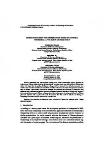
Fig. 1. Implementation of a DT LTI system using delays, adders and multipliers.
Then, Fig. 2. Matrices
and
of the redundant implementation.
(11) (12) A problem arises if has only one nonzero entry (because in such case we cannot simultaneously solve for and ). Notice, however, that such a case implies that the error has affected one of the added (“parity”) state variables. Furthermore, since has been set to zero, these errors will only affect the calculation of the added state variables and will have no influence on the rest of the system [see eq. (10)]. In particular, to correct we can set it to be
where is given by the top entries of (since the original state variables have not been affected).
In this section we borrow an example from [8] to illustrate the redundant implementations and decoding approach that was developed in Section V. More specifically, we consider how to detect and identify two or less errors in the system of Figure 1 (which is implemented using delays, adders and multipliers that are interconnected in a circuit that has delay-free paths of unit length [8]). The state evolution of system is given by
(13)
To be able to detect and identify up to two errors we use four extra state variables ( ). The Vandermonde transformation matrix and the diagonal matrix in the Theorem V.2 are chosen to be diag . Matrix
for all
in
With these choices and with the coupling matrix set to zero for simplicity, we obtain the redundant implementation with state evolution
where matrixes
and
are shown in Figure 2.
The syndrome matrix for non-concurrent error detection and correction in this system is given by
C. Example
with
Note that, as required by Condition 3 of Theorem V.2, the above choices ensure that and all ’s are nonzero, all ’s are unique and that all pairs of in satisfy the following:
is set to
where The modified syndrome matrix is given by
.
Suppose that the system operates in the interval . (We choose for illustration purposes; in principle, can be extended to any finite , as long as our system can handle the finite precision limitations of the arithmetic involved.) As an example, let us consider two transient faults that take place as follows: 1) Fault takes place during time step , originally corrupting the th state variable with an additive initial error of value ; 2) Fault takes place during time step , originally corrupting the th state variable with an additive initial error of value . The syndrome at time step
is given by
and the modified syndrome is given by
(the syndrome does not depend on the actual input sequence that is applied to the system, as long as the faults take place at the same time steps and originally affect the same state variables with the same initial additive errors). The ’s are obtained by considering the solution to the following matrix equation:
Solving the above, we find that and ; therefore, we need to find the roots of the polynomial
by trying all possible roots are and
(
) values, we find that the , which implies that
We conclude that a fault affected the th state variable during time step ( ) and that a fault affected the th state variable during time step ( ). The only remaining question is to determine the magnitudes of the initial errors. To achieve this, we just use
We find that and and conclude that there have been two faults: one affecting the th state variable by an additive error of at time step and one affecting the th state variable by an additive error of at time step .
R EFERENCES [1] P. E. Beckmann and B. R. Musicus. Fault-tolerant round-robin A/D converter system. IEEE Transactions on Circuits and Systems, 38(12):1420– 1429, December 1991. [2] P. E. Beckmann and B. R. Musicus. Fast fault-tolerant digital convolution using a polynomial residue number system. IEEE Transactions on Signal Processing, 41(7):2300–2313, July 1993. [3] R. E. Blahut. Algebraic Codes for Data Transmission. Cambridge University Press, Cambridge, UK, 2002. [4] A. Chatterjee and M. d’Abreu. The design of fault-tolerant linear digital state variable systems: Theory and techniques. IEEE Transactions on Computers, 42(7):794–808, July 1993. [5] A. M. Cohen. Numerical Analysis. Wiley, New York, 1973. [6] G. H. Golub and C. F. Van Loan. Matrix Computations. The John Hopkins University Press, Baltimore, Maryland, 1983. [7] C. N. Hadjicostis. Coding Approaches to Fault Tolerance in Dynamic Systems. PhD thesis, EECS Department, Massachusetts Institute of Technology, Cambridge, Massachusetts, 1999. [8] C. N. Hadjicostis. Coding Approaches to Fault Tolerance in Combinational and Dynamic Systems. Kluwer Academic Publishers, Boston, Massachusetts, 2002.
[9] C. N. Hadjicostis and G. C. Verghese. Structured redundancy for fault tolerance in LTI state-space models and Petri nets. Kybernetika, 35(1):39– 55, January 1999. [10] K.-H. Huang and J. A. Abraham. Algorithm-based fault tolerance for matrix operations. IEEE Transactions on Computers, 33(6):518–528, June 1984. [11] B.W. Johnson. Design and Analysis of Fault-Tolerant Digital Systems. Addison-Wesley, Reading, Massachusetts, 1989. [12] J.-Y. Jou and J. A. Abraham. Fault-tolerant matrix arithmetic and signal processing on highly concurrent parallel structures. Proceedings of the IEEE, 74(5):732–741, May 1986. [13] J.-Y. Jou and J. A. Abraham. Fault-tolerant FFT networks. IEEE Transactions on Computers, 37(5):548–561, May 1988. [14] T. Kailath. Linear Systems. Prentice-Hall, Englewood Cliffs, New Jersey, 1980. [15] D. G. Luenberger. Introduction to Dynamic Systems: Theory, Models, & Applications. John Wiley & Sons, New York, 1979. [16] V. S. S. Nair and J. A. Abraham. Real-number codes for fault-tolerant matrix operations on processor arrays. IEEE Transactions on Computers, 39(4):426–435, April 1990. [17] A. V. Oppenheim and R. W. Schafer with J. R. Buck. Discrete-Time Signal Processing. Prentice Hall, Englewood Cliffs, New Jersey, 1999. [18] D. K. Pradhan. Fault-Tolerant Computer System Design. Prentice Hall, Englewood Cliffs, New Jersey, 1996. [19] T. R. N. Rao and E. Fujiwara. Error-Control Coding for Computer Systems. Prentice-Hall, Englewood Cliffs, New Jersey, 1989. [20] G. R. Redinbo. Generalized algorithm-based fault tolerance: Error correction via Kalman estimation. IEEE Transactions on Computers, 47(6):639–655, June 1998. [21] J. Riordan. An Introduction to Combinatorial Analysis. John Wiley & Sons, New York, 1958. [22] R. A. Roberts and C. T. Mullis. Digital Signal Processing. AddisonWesley, Reading, Massachusetts, 1987. [23] J. Rosenthal and F. V. York. BCH convolutional codes. IEEE Transactions on Information Theory, 45(6):1833–1844, September 1999. [24] A. Roy-Chowdhury and P. Banerjee. Algorithm-based fault location and recovery for matrix computations on multiprocessor systems. IEEE Transactions on Computers, 45(11):1239–1247, November 1996. [25] D.P. Siewiorek and R.S. Swarz. Reliable Computer Systems: Design and Evaluation. A.K. Peters, Natick, Massachusetts, 1998. [26] J.-L. Sung and G. R. Redinbo. Algorithm-based fault tolerant synthesis for linear operations. IEEE Transactions on Computers, 45(4):425–437, April 1996. [27] J. von Neumann. Probabilistic Logics and the Synthesis of Reliable Organisms from Unreliable Components. Princeton University Press, Princeton, New Jersey, 1956. [28] S. B. Wicker. Error Control Systems. Prentice Hall, Englewood Cliffs, New Jersey, 1995. Christoforos N. Hadjicostis (M’95) received S.B. degrees in Electrical Engineering, in Computer Science and Engineering, and in Mathematics, the M.Eng. degree in Electrical Engineering and Computer Science in 1995, and the Ph.D. degree in ElecPLACE trical Engineering and Computer Science in 1999, PHOTO all from the Massachusetts Institute of TechnolHERE ogy, Cambridge, MA. In August 1999 he joined the Faculty at the University of Illinois at UrbanaChampaign where he is currently an Assistant Professor with the Department of Electrical and Computer Engineering and a Research Assistant Professor with the Coordinated Science Laboratory. His research interests include systems and control, fault-tolerant computational architectures, and fault diagnosis and management in large-scale systems and networks. Dr. Hadjicostis received the Faculty Early Development (CAREER) award from the National Science Foundation in February 2001. As a graduate student, he served as president of the MIT Chapter of HKN, received the Harold L. Hazen Teaching Award and the Ernst A. Guillemin Thesis Prize, and received fellowships from the National Semiconductor Corporation and the Grass Instrument Company. Dr. Hadjicostis is a member of Eta Kappa Nu, Sigma Xi, and the IEEE.