Non-Convex Phase Retrieval Algorithms and

Non-Convex Phase Retrieval Algorithms and Performance Analysis

A DISSERTATION SUBMITTED TO THE FACULTY OF THE GRADUATE SCHOOL OF THE UNIVERSITY OF MINNESOTA BY

Gang Wang

IN PARTIAL FULFILLMENT OF THE REQUIREMENTS FOR THE DEGREE OF DOCTOR OF PHILOSOPHY

Prof. Georgios B. Giannakis, Advisor

April, 2018

c Gang Wang 2018

ALL RIGHTS RESERVED

Acknowledgments There are so many people to whom I wish to acknowledge and thank for making my past four years at the University of Minnesota (UMN) the most rewarding and enlightening journey of my life so far, and for this thesis in particular. First and foremost, my deepest gratitude goes to my advisor Prof. Georgios B. Giannakis. I am very grateful to him for such an exciting and fruitful experience during my PhD studies. His advice and feedback on the formalization, investigation, and presentation of original research has been extraordinary to me by all means. His invaluable guidance as well as constant encouragement through dedicating extensive amounts of time has not only made me a better researcher, but also a better person. His vision and enthusiasm about innovative research and beyond, his broad and deep knowledge, and his unbounded energy have constantly been a true inspiration for me. He has also provided me with phenomenal environments for conducting research, and (because of him) I have been very fortunate to be always surrounded by other wonderful students and colleagues. This thesis would have not been possible without his support. I would also like to extend my sincerest appreciation to Profs. Jie Chen and Jian Sun at the Beijing Institute of Technology (BIT), for introducing me to the world of academic research at the very beginning of my graduate studies at BIT, for their true understanding of my concerns throughout the course of my PhD at BIT as well as at UMN, and for many other reasons which cannot be expressed in the space provided here. Due thanks go to Profs. Mostafa Kaveh, Yousef Saad, and Mehmet Akçakaya for agreeing to serve on my committee as well as all their valuable comments and feedback on my research and thesis. Thanks also go to other professors in the Departments of Electrical Engineering and Computer Science whose graduate level courses helped me build the necessary background to embark on this journey. During my PhD studies, I had the opportunity to collaborate with several excellent individuals, i

and I have greatly benefited from their critical thinking, brilliant ideas, and vision. Particularly, I would like to express my gratitude to Prof. Seung-Jun Kim who was patient enough to train me in the first couple of years at UMN, and Prof. Vassilis Kekatos, with whom we had great research collaboration. I would also like to extend my due credit and warmest thanks to Profs. Mehmet Akçakaya, Antonio J. Conejo (OSU), Yonina C. Eldar (Technion), Yousef Saad, and Nikos D. Sidiropoulos (UVA) for their insightful input to our fruitful collaborations. The material in this thesis has also benefited from discussions with current and former members of the SPiNCOM group at UMN: Dr. Brian Baingana, Prof. Juan-Andrés Bazerque, Dimitris Berberidis, Dr. Jia Chen, Tianyi Chen, Dr. Emiliano Dall’Anese, Vassilis Ioannidis, Georgios V. Karanikolas, Donghoon Lee, Prof. Geert Leus, Bingcong Li, Prof. Qing Ling, Meng Ma, Dr. Morteza Mardani, Prof. Antonio G. Marqués, Prof. Gonzalo Mateos, Dr. Athanasios Nikolakopoulos, Prof. Daniel Romero, Alireza Sadeghi, Fatemeh Sheikholeslami, Yanning Shen, Prof. Konstantinos Slavakis, Panagiotis Traganitis, Dr. Yunlong Wang, Liang Zhang, Prof. Yu Zhang, and Prof. Hao Zhu. I am truly grateful to these people for their continuous help. I would also wish to acknowledge the grants that support financially our research. I am not forgetting my friends, some of which I have already mentioned above, both the ones here in Minneapolis, and my old friends that are far away in China, in particular: Yongjian Cai, Kexin Guo, Shuai He, Haoji Hu, Kejun Huang, Mingyi Hong, Meng Li, Cheng Qian, Yunmei Shi, Hanghai Tian, Jiaxiang Yan, Bo Yang, and Ahmed S. Zamzam. Last but not least, I am eternally grateful to my parents, Fengming Wang and Mingju Zhang, who encouraged me and gave me every learning opportunity they could think of. Without you, I would not be standing here today.

Gang Wang, Minneapolis, March 10, 2018.

ii

Dedication This dissertation is dedicated to my family for their unconditional love and support.

iii

Abstract High-dimensional signal estimation plays a fundamental role in various science and engineering applications, including optical and medical imaging, wireless communications, and power system monitoring. The ability to devise solution procedures that maintain high computational and statistical efficiency will facilitate increasing the resolution and speed of lensless imaging, identifying artifacts in products intended for military or national security, as well as protecting critical infrastructure including the smart power grid. This thesis contributes in both theory and methods to the fundamental problem of phase retrieval of high-dimensional (sparse) signals from magnitude-only measurements. Our vision is to leverage exciting advances in non-convex optimization and statistical learning to devise algorithmic tools that are simple, scalable, and easy-to-implement, while being computationally and statistically (near-)optimal. Phase retrieval is approached from a non-convex optimization perspective. To gain statistical and computational efficiency, the magnitude data (instead of the intensities) are fitted based on the least-squares or maximum likelihood criterion, which leads to optimization models that trade off smoothness for ‘low-order’ non-convexity. To solve the resultant challenging nonconvex and non-smooth optimization, the present thesis introduces a two-stage algorithmic framework, that is termed amplitude flow. The amplitude flows start with a careful initialization, which is subsequently refined by a sequence of regularized gradient-type iterations. Both stages are lightweight, and they scale well with problem dimensions. Due to the highly non-convex landscape, judicious gradient regularization techniques such as trimming (i.e., truncation) and iterative reweighting are devised to boost the exact phase recovery performance. It is shown that successive iterates of the amplitude flows provably converge to the global optimum at a geometric rate, corroborating their efficiency in terms of computational, storage, and data resources. The amplitude flows are also demonstrated to be stable vis-à-vis additive noise. Sparsity plays a critical role in many fields - what has led to the upsurge of research referred to as compressive sampling. In diverse applications, the signal is naturally sparse or admits a sparse representation after some known and deterministic linear transformation. This thesis also accounts for phase retrieval of sparse signals, by putting forth sparsity-cognizant amplitude flow variants. Although analysis, comparisons, and corroborating tests focus on non-convex phase retrieval in this thesis, a succinct overview of other areas is provided to highlight the universality of the novel algorithmic framework to a number of intriguing future research directions. iv

Contents Acknowledgments

i

Dedication

iii

Abstract

iv

List of Tables

viii

List of Figures 1

2

ix

Introduction

1

1.1

The Phase Retrieval Problem . . . . . . . . . . . . . . . . . . . . . . . . . . .

1

1.2

Motivation and Context . . . . . . . . . . . . . . . . . . . . . . . . . . . . . .

2

1.2.1

Uniqueness of the phase retrieval problem . . . . . . . . . . . . . . . .

3

1.2.2

Algorithmic developments . . . . . . . . . . . . . . . . . . . . . . . .

4

1.2.3

Applications of phase retrieval . . . . . . . . . . . . . . . . . . . . . .

6

1.3

Thesis Outline and Contributions . . . . . . . . . . . . . . . . . . . . . . . . .

9

1.4

Notational Conventions . . . . . . . . . . . . . . . . . . . . . . . . . . . . . .

11

Phase Retrieval via Amplitude Flow

13

2.1

Non-convex Optimization Models . . . . . . . . . . . . . . . . . . . . . . . .

13

2.2

Truncated Amplitude Flow . . . . . . . . . . . . . . . . . . . . . . . . . . . .

14

2.2.1

Truncated gradient iterations . . . . . . . . . . . . . . . . . . . . . . .

15

2.2.2

Orthogonality-promoting initialization . . . . . . . . . . . . . . . . . .

20

Main Results . . . . . . . . . . . . . . . . . . . . . . . . . . . . . . . . . . .

26

2.3

v

3

4

5

2.4

Numerical Experiments . . . . . . . . . . . . . . . . . . . . . . . . . . . . . .

27

2.5

Proofs . . . . . . . . . . . . . . . . . . . . . . . . . . . . . . . . . . . . . . .

32

2.5.1

Constant relative error by initialization . . . . . . . . . . . . . . . . .

32

2.5.2

Exact recovery from noiseless data . . . . . . . . . . . . . . . . . . . .

35

Phase Retrieval via Iteratively Reweighted Algorithms

43

3.1

Reweighted Amplitude Flow . . . . . . . . . . . . . . . . . . . . . . . . . . .

44

3.1.1

Weighted maximal correlation initialization . . . . . . . . . . . . . . .

44

3.1.2

Adaptively reweighted gradient flow . . . . . . . . . . . . . . . . . . .

48

3.1.3

Parameters of the algorithm . . . . . . . . . . . . . . . . . . . . . . .

50

3.2

Main Results . . . . . . . . . . . . . . . . . . . . . . . . . . . . . . . . . . .

50

3.3


52

3.4

Proofs . . . . . . . . . . . . . . . . . . . . . . . . . . . . . . . . . . . . . . .

54

3.4.1

Initialization performance . . . . . . . . . . . . . . . . . . . . . . . .

54

3.4.2

Exact Phase Retrieval from Noiseless Data . . . . . . . . . . . . . . .

56

Phase Retrieval via Stochastic Optimization

60

4.1

Stochastic Truncated Amplitude Flow . . . . . . . . . . . . . . . . . . . . . .

60

4.1.1

Variance-reducing orthogonality-promoting initialization . . . . . . . .

62

4.1.2

Stochastic truncated gradient iterations . . . . . . . . . . . . . . . . .

65

4.2

Main Results . . . . . . . . . . . . . . . . . . . . . . . . . . . . . . . . . . .

67

4.3


68

4.4

Proofs . . . . . . . . . . . . . . . . . . . . . . . . . . . . . . . . . . . . . . .

72

Phase Retrieval of Sparse Signals

79

5.1

Sparse Phase Retrieval . . . . . . . . . . . . . . . . . . . . . . . . . . . . . .

80

5.2

Sparse Truncated Amplitude Flow . . . . . . . . . . . . . . . . . . . . . . . .

82

5.2.1

Sparse orthogonality-promoting initialization . . . . . . . . . . . . . .

82

5.2.2

Thresholded truncated gradient iterations . . . . . . . . . . . . . . . .

84

5.3

Main Results . . . . . . . . . . . . . . . . . . . . . . . . . . . . . . . . . . .

86

5.4


87

5.5

Proofs . . . . . . . . . . . . . . . . . . . . . . . . . . . . . . . . . . . . . . .

91

vi

6

Summary and Future Directions

99

6.1

Thesis Summary . . . . . . . . . . . . . . . . . . . . . . . . . . . . . . . . .

99

6.2

Future Research . . . . . . . . . . . . . . . . . . . . . . . . . . . . . . . . . . 101 6.2.1

Convolutional phase retrieval . . . . . . . . . . . . . . . . . . . . . . . 101

6.2.2

Learning convolutional neural networks . . . . . . . . . . . . . . . . . 101

6.2.3

Exact power system state recovery . . . . . . . . . . . . . . . . . . . . 102

References

104

Appendix A. Proofs for Chapter 2

118

A.1 Proof of Lemma 1 . . . . . . . . . . . . . . . . . . . . . . . . . . . . . . . . . 118 A.2 Proof of Lemma 2 . . . . . . . . . . . . . . . . . . . . . . . . . . . . . . . . . 120 A.3 Proof of Lemma 3 . . . . . . . . . . . . . . . . . . . . . . . . . . . . . . . . . 122 A.4 Proof of Lemma 5 . . . . . . . . . . . . . . . . . . . . . . . . . . . . . . . . . 127 A.5 Proof of Lemma 6 . . . . . . . . . . . . . . . . . . . . . . . . . . . . . . . . . 131 Appendix B. Proofs for Chapter 3

134

B.1 Proof of Lemma 8 . . . . . . . . . . . . . . . . . . . . . . . . . . . . . . . . . 134 B.2 Proof of Lemma 9 . . . . . . . . . . . . . . . . . . . . . . . . . . . . . . . . . 135 B.3 Proof of Proposition 9 . . . . . . . . . . . . . . . . . . . . . . . . . . . . . . . 138 B.4 Proof of Lemma 15 . . . . . . . . . . . . . . . . . . . . . . . . . . . . . . . . 141 B.5 Proof of Lemma 16 . . . . . . . . . . . . . . . . . . . . . . . . . . . . . . . . 142 Appendix C. Proofs for Chapter 5

145

C.1 Proof of Lemma 10 . . . . . . . . . . . . . . . . . . . . . . . . . . . . . . . . 145 Appendix D. Supporting Lemmas

149

vii

List of Tables 4.1

Computational Complexity of Different Algorithms . . . . . . . . . . . . . . .

viii

61

List of Figures 1.1

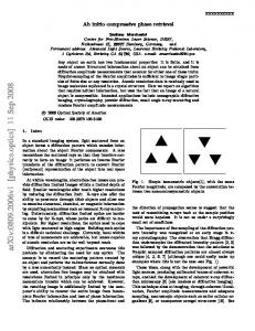
Schematic diagram of the experimental setup for coherent diffraction imaging: A coherent wave diffracts from a sample of Fe/Fe2 O3 , and generates a far-field diffraction pattern which corresponds to the modulus of the Fourier transform of the sample. . . . . . . . . . . . . . . . . . . . . . . . . . . . . . . . . . . . .

1.2

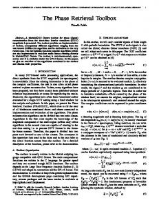
The time-slotted frame diagram of the RSS/CQI feedback system adapted from [96]. . . . . . . . . . . . . . . . . . . . . . . . . . . . . . . . . . . . . . . . .

2.1

7 8

Geometric description of the proposed truncation rule on the i-th gradient component involving aTi x = ψi , where the red dot denotes the solution x and the black one is the origin. Hyperplanes aTi z = ψi and aTi z = 0 (of z ∈ Rn ) passing through points z = x and z = 0, respectively, are shown. . . . . . . .

2.2

17

Empirical success rate from the same truncated spectral initialization under the real Gaussian model. . . . . . . . . . . . . . . . . . . . . . . . . . . . . . . .

21

2.3

Ordered squared normalized inner-product for pairs x and ai . . . . . . . . . .

22

2.4

Relative initialization error versus m/n. Left: Noiseless real Gaussian model; Right: Noisy real Gaussian model with σ 2 = 0.22 kxk2 .

2.5

. . . . . . . . . . . .

24

Relative initialization error using noise-free (solid) and noisy (dotted) data. Left: Real Gaussian model with σ 2 = 0.22 kxk2 ; Right: Complex Gaussian model with σ 2 = 0.22 kxk2 . . . . . . . . . . . . . . . . . . . . . . . . . . . . . . . .

2.6

Relative initialization errors of solving (2.15) via the Lanczos method and solving (2.18) via the power method. . . . . . . . . . . . . . . . . . . . . . . . . . . .

2.7

27 28

Empirical success rate. Left: Real Gaussian model; Right: Complex Gaussian model.

. . . . . . . . . . . . . . . . . . . . . . . . . . . . . . . . . . . . . .

29

2.8

Relative error versus iteration for TAF with m = 2n − 1. . . . . . . . . . . . .

30

2.9

Relative MSE versus SNR for TAF under the amplitude-based noisy data model. 31 ix

2.10 Empirical success rate using the truncated spectral and the orthogonality-promoting initializations.

. . . . . . . . . . . . . . . . . . . . . . . . . . . . . . . . . .

31

2.11 The recovered Milky Way Galaxy images after i) truncated spectral initialization (top); ii) orthogonality-promoting initialization (middle); and iii) 100 TAF gradient iterations refining the orthogonality-promoting initialization (bottom).

42

3.1

Relative initialization error for the real Gaussian model.

47

3.2

Relative error versus γ for the proposed initialization and m = 2n − 1 fixed

. . . . . . . . . . . .

using the real Gaussian model. . . . . . . . . . . . . . . . . . . . . . . . . . . 3.3 3.4 4.1 4.2

Function value

L(z T )

evaluated at the returned RAF estimate

zT

51

for 200 trials

with n = 2, 000 and m = 2n − 1 = 3, 999. . . . . . . . . . . . . . . . . . . .

52

Real Gaussian model. Left: Empirical success rate; Right: NMSE vs. SNR. . . Rigengaps δ of Y¯0 ∈ Rn×n . Left: Real Gaussian model; Right: Complex

53

Gaussian model.

62

. . . . . . . . . . . . . . . . . . . . . . . . . . . . . . . . .

Error evolution of the iterates for solving problem (4.1) with step size η = 1. Left: Noiseless real Gaussian model with m = 2n−1; Right: Noiseless complex Gaussian model with and m = 4n − 4.

4.3

. . . . . . . . . . . . . . . . . . . . .

69

Empirical success rate under the same orthogonality-promoting initialization. Left: Noiseless real Gaussian model; Right: Noiseless complex Gaussian model. 69

4.4

Relative error versus iterations under the same orthogonality-promoting initialization. Left: Noiseless real Gaussian model; Right: Noiseless complex Gaussian model.

4.5

. . . . . . . . . . . . . . . . . . . . . . . . . . . . . . . . .

70

Relative error versus iterations with n = 1, 000 and m/n = 5. Left: Noisy real Gaussian model; Right: Noisy complex Gaussian model. . . . . . . . . . . . .

4.7

70

Empirical success rate. Left: Noiseless real Gaussian model; Right: Noiseless Gaussian model.

4.6

. . . . . . . . . . . . . . . . . . . . . . . . . . . . . . . . .

72

Recovered images after: the variance-reducing orthogonality-promoting initialization stage (top panel), and the STAF refinement stage (bottom panel) on the Milky Way Galaxy image using K = 8 random masks. . . . . . . . . . . . . .

73

5.1

Empirical success rate versus m/n. . . . . . . . . . . . . . . . . . . . . . . .

88

5.2

Empirical success rate versus sparsity level k. . . . . . . . . . . . . . . . . . .

89

5.3

Convergence behavior for noisy data with n = 1, 000, m = 3, 000, and k = 10.

89

5.4

Relative MSE versus SNR for SPARTA with the AWGN model. . . . . . . . .

90

x

5.5

Relative MSE versus iteration count for SPARTA in the complex setting. . . . .

91

B.1 The expectation E[wi ] as a function of ρ over [−1, 1]. . . . . . . . . . . . . . . 144

xi

Chapter 1

Introduction 1.1

The Phase Retrieval Problem

Detecting visible light and radiation of high frequencies relies on energy intensity measurements of the sought radiating field. The field on the other hand is can be characterized by a complex function, comprising its modulus and phase parameters. The intensity is proportional to the square of the modulus, but the phase information is lost at the energy detector [16]. Consider for example an image formation experiment. Suppose that the field in the object (primary) space is denoted by E(p). If an image indexed by i is formed, the field in the image space is given by Ei (p0 ). In addition, at a large enough distance from the imaging plane, the complex functions E(p), and Ei (p0 ) are known to be related through Fourier transform relations, determination of one of which provides the other. In physical scattering experiments however, one can only measure |Ei (p0 )|. In general, the modulus data |Ei (p0 )| provides only geometrical information concerning the object of interest. To recover the image, namely to determine the structure of the object, one has to recover the missing phases of Ei (p0 ) first, which is known as the phase retrieval problem [55]. To set up the phase retrieval problem mathematically, this thesis focuses on the discretized one-dimensional (1D) setting. Suppose we have an object of interest described by x ∈ Cn , and that we would like to measure hai , xi for some known sampling vectors ai ∈ Cn , but only have access to the modulus of the linear transformations, namely yi = |hai , xi|2 ,

i = 1, 2, . . . , m. 1

(1.1)

2 The goal here is to recover the missing phase of the linear transformations hai , xi, which is known as the (generalized) phase retrieval problem. In the original phase retrieval problem, the sampling vectors ai correspond to rows of the discrete Fourier transform (DFT) matrix of suitable dimensions, in which case one is tasked with recovering a signal vector from the modulus of its Fourier transform. It is clear that once the phase becomes available, one can easily find the object x by solving linear equations. Succinctly stated, we are interested in solving systems of quadratic equations of the form find z ∈ Cn subject to yi = |hai , zi|2 ,

(1.2a) i = 1, 2, . . . , m

(1.2b)

where z ∈ Cn is the decision vector, {ai ∈ Cn } are the known sampling vectors, and {yi ∈ R} are the observed data.

1.2

Motivation and Context

The phase problem appears in many fields of science and engineering [47]. X-ray crystallography is one such field which, as is well known, led to the discovery of the double helix structure of DNA [55]. Besides X-ray crystallography, other relevant application domains include optics [86], array and high-power coherent diffractive imaging [25], astronomical imaging [46], ptychography [144], and microscopy [85]. Similar problems are also encountered in areas such as acoustics [7], channel estimation in wireless communications [2, 96], computational biology [114], speech processing [1], quantum mechanics [98], and quantum information [38]. It has been shown that reconstructing a discrete, finite-duration signal from its Fourier transform magnitude is generally NP-complete [102]. Even checking quadratic feasibility (i.e., whether a solution to a given quadratic system of the form (1.2) exists or not) is itself an NP-hard problem [57, Thm. 2.6]. Therefore, despite its simple form and practical relevance across various fields, tackling the quadratic system in (1.2) is challenging and NP-hard in general. The problem in (1.2) constitutes an instance of non-convex quadratic programming. Specifically for real ai and x, problem (1.2) can be understood as a combinatorial optimization since one seeks a series of signs {si = ±1}m i=1 , such that the solution to the system of linear equations √ hai , xi = si ψi , where ψi := yi , obeys the given quadratic system. Evidently, there are a total

3 of 2m different combinations of

{si }m i=1 ,

among which only two lead to x up to a global sign.

The complex case becomes even more complicated, where instead of a set of signs {si }m i=1 , one must determine a collection of unimodular complex scalars {σi ∈ C}m i=1 . Special cases with ai > 0 (entry-wise inequality), x2i = 1, and yi = 0, 1 ≤ i ≤ m, correspond to the so-called stone problem [10, Sec. 3.4.1].

1.2.1

Uniqueness of the phase retrieval problem

We first review some results from the literature that give conditions under which the phase retrieval problem (1.2) has a unique solution (up to a global unimodular constant). In this process, the different models for the sampling vectors ai that have been commonly used will also become clear. To that end, collect all sampling vectors ai in the m × n matrix A := [a1 · · · am ]H , and concatenate all modulus squares yi to form the data vector y := [y1 · · · ym ]T , which collectively lead to the more compact matrix-vector representation y = |Ax|2 , where the modulus operator | · | should be understood entry-wise. Let us start with the uniqueness of Fourier phase retrieval, in which one takes measurements of the form y = |F x|2

(1.3)

where F ∈ Cn×n corresponds to the DFT matrix. It is clear from signal processing that there are trivial ambiguities in the Fourier phase retrieval problem due to e.g., i. phase shift (x[i] → x[i] · ejθ ); ii. spatial shift (x[i] → x[i + i0 ]); and iii. conjugate inversion (x[i] → x[−i]) each or any combination of which conserves Fourier magnitude, namely yields the same modulus data y. Beyond trivial ambiguities, it has been shown that unique reconstruction of signals is impossible using Fourier modulus measurements [58]. To see this, assign each magnitude measurement yi an arbitrary phase θi , and a direct inverse Fourier transform would yield a solution that also adheres to the data (1.3). For the Fourier phase retrieval problem to be uniquely solvable (up to trivial ambiguities), a number of approaches have been suggested, a sample of which are outlined next [108, 61].

4 • Additional constraints on the signal vector. One common assumption is that the signal vector x has bounded support. However, this assumption does not overcome the illposeness of the 1D Fourier phase retrieval, but it is helpful when it comes to retrieving the phase of 2D or 3D signals. Another structural assumption is that x is sparse in the sense that only a small fraction of entries are nonzero. In this case one may also be able to recover x using only a few Fourier measurements, namely a number m < n of equations as in (1.3) [56]. Another possibility is when nonnegative entries of the signal vector are constrained to be nonnegative, which clearly holds true in imaging applications [47, 107]. • Oversampled DFT. An alternative is to have additional redundant measurements. A common strategy is to sample the signal in the continuous domain at a finer scale. That is, instead of using frequencies ωi = 2πi/n, one can use ωi0 = 2πi/m for i = 1, 2, . . . , m, and m ≥ n. Using the argument that the autocorrelation function of any signal is twice the size of the signal itself, it has been proved that phases of real signals can be uniquely retrieved from the Fourier measurements if and only if one oversamples by a factor of two [85]. Let us now turn our attention to the generalized phase retrieval, where one considers general measurement vectors ai that do not necessarily correspond to rows of DFT matrices. To this end, let us first introduce the notion of generic measurements. If A corresponds to a point in a non-empty Zariski open subset of Cm×n /Rm×n , the measurements y = |Ax|2 are said to be generic [37]. When both x and ai are real, it has been shown in [8] that m = 2n − 1 generic measurements are necessary for ensuring injectivity of the mapping z → |Az|2 , and m ≥ 2n − 1 generic measurements are also sufficient for injectivity. For example, m ≥ 2n − 1 Gaussian random measurements are injective with probability one. In the complex case, a line of research has established that the minimum number of generic measurements required for injectivity is smaller than 4n − 4, and likewise, when m ≥ 4n − 4 generic measurements are available, the mapping is injective with probability one [37].

1.2.2

Algorithmic developments

Adopting the maximum likelihood criterion, the task of recovering x from data yi observed in additive white Gaussian noise (AWGN) can be recast as that of minimizing the intensity-based

5 empirical loss [22, 44] m

1 X 2 2 minimize f (z) := y − |ha , zi| . i i z∈Cn 2m

(1.4)

i=1

An alternative is to consider the Poisson likelihood [32] m

1 X minimize h(z) := − yi log(|hai , zi|2 ) + |hai , zi|2 . z∈Cn 2m

(1.5)

i=1

Unfortunately, both (1.4) and (1.5) are non-convex. Minimizing non-convex cost functions, which may exhibit many stationary points, is in general NP-hard [89]. In fact, even checking whether a given point is a local minimum or establishing convergence to a local minimum turns out to be NP-complete [89]. Previous approaches to solving (1.4) or (1.5) fall under two categories: non-convex and convex ones. Popular non-convex solvers include alternating projection such as GerchbergSaxton [48] and Fineup [47], AltMinPhase [91], (Truncated) Wirtinger flow (WF/TWF) [22, 32, 111], and trust-region methods [117]. Convex counterparts, on the other hand, rely on the so-called matrix-lifting technique or Shor’s semidefinite relaxation to obtain the solvers abbreviated as PhaseLift [20], PhaseCut [121], and CoRK [59]. Another line of convex relaxation [51, 49, 6, 54, 41] reformulates phase retrieval as a sparse signal recovery problem, and solves a linear program in the natural parameter vector domain. Although exact signal recovery can be established assuming an accurate enough anchor vector, its empirical performance is often not competitive with state-of-the-art phase retrieval approaches. Additional related approaches can be found in [59, 34, 146, 27, 11, 77, 5, 43, 141, 83, 33, 95, 63, 120, 40, 82, 118, 11, 31, 150, 103, 78, 87]. Interested readers can also access Matlab implementations in [26] for a sample of the aforementioned as well as our proposed phase retrieval solvers. In terms of sample complexity, it has been proven that1 O(n) noise-free measurements suffice for uniquely determining a general signal [44]. It is also self-evident that recovering a general n-dimensional x requires at least O(n) measurements. Convex approaches enable exact recovery from the optimal bound O(n) of noiseless measurements [20]; they are based 1 The notation φ(n) = O(g(n)) or φ(n) & g(n) (respectively, φ(n) . g(n)) means there exists a numerical constant c > 0 such that φ(n) ≤ cg(n), while φ(n) g(n) means φ(n) and g(n) are orderwise equivalent.

6 on solving a semidefinite program with a matrix variable of size n × n, thus incurring worstcase computational complexity on the order of O(n4.5 ) [121] that does not scale well with n. Upon exploiting the problem structure, O(n4.5 ) can be reduced to O(n3 ) [121]. Solving for vector variables, non-convex approaches on the other hand, enjoy significantly improved computational performance. Adopting a spectral initialization commonly employed in matrix completion [69], AltMinPhase establishes exact recovery with sample complexity O(n log3 n) with resampling [91]. The WF iteratively refines the spectral initial estimate by means of gradient-type updates, which can be approximately interpreted as a variant of stochastic gradient descent [22], [111]. The follow-up TWF improves upon WF through a truncation procedure to separate gradient components of excessively extreme (large or small) sizes. Likewise, due to the heavy tails present in the initialization stage, data {yi }m i=1 are pre-screened to yield improved initial estimates in the so-termed truncated spectral initialization method [32]. The WF allows exact recovery from O(n log n) measurements in O(mn2 log(1/)) time/flops to yield an -accurate solution for any given > 0 [22], while TWF advances these to O(n) measurements and O(mn log(1/)) time [32]. It is also worth mentioning that when m ≥ Cn log3 n for some sufficiently large positive constant C, the objective function in (1.4) has been shown to admit benign geometric structure that allows certain iterative algorithms (e.g., trust-region methods) to efficiently find a global minimizer with random initializations [117].

1.2.3

Applications of phase retrieval

In this subsection, we discuss two applications of phase retrieval. The goal here is to demonstrate how the Fourier phase retrieval emerges naturally in diverse imaging applications, and how the generalized phase retrieval (with general measurements) can be instrumental to real-world applications. Optical imaging In optical imaging, researchers constantly wish to increase resolution so that details can be imaged at a finer scale. Eventually, successful imaging of large protein complexes and biological specimens would further advance the understanding of bio-chemical activities at the molecular level. Phaseless imaging has also become critical in emerging national security applications

7

Figure 1.1: Schematic diagram of the experimental setup for coherent diffraction imaging: A coherent wave diffracts from a sample of Fe/Fe2 O3 , and generates a far-field diffraction pattern which corresponds to the modulus of the Fourier transform of the sample. such as monitoring electronic products intended for military or infrastructure use, where the goal is to ensure such products are clear of secret backdoors granting foreign governments cyber access to vital US infrastructure. The limitation of lens-type imaging devices is that the required optical components such as mirrors and lenses are in general very difficult to construct at short wavelengths, so increasing resolution becomes rather difficult for lens-type imaging devices. On the other hand, phaseless imaging that is based on the Fourier phase retrieval offers a promising alternative for recovery of phase structure because it does not require such optical components. Below, we briefly overview the history of algorithmic phase retrieval in optical imaging. The use of algorithmic phase retrieval was first suggested in X-ray diffraction microscopy by Sayre in a seminal contribution back in 1952 [104]. Later in 1978, Fienup developed an approach to empirically recover the phase information of 2D images from the modulus of their Fourier transform leveraging prior knowledge such as non-negativity and known support of signal values [47]. The revival of algorithmic phase retrieval around 2000 was due mainly to the successful experimental recording and reconstruction of a diffraction pattern of a non-crystalline object using the so-called coherent diffraction imaging [84]. Figure 1.1 depicts an illustrative experimental setup2 , where the diffraction patterns are (proportional to) the intensities of the Fourier transform of the object [108]. There techniques have recently been employed to image 2

This figure is adapted from https://www6.slac.stanford.edu/.

8

Figure 1.2: The time-slotted frame diagram of the RSS/CQI feedback system adapted from [96]. small particles in diverse applications, including nano-particles, biomaterials, specimen, and electronic circuits [108, 112]. Wireless channel estimation Another interesting application of algorithmic phase retrieval lies in the estimation of a communication channel. Channel estimation is a critical task in any wireless communication system, and 5G massive multiple-input multiple-output (MIMO) systems, in particular [72] - because the receiver must estimate and feed back to the transmitter a high-dimensional multiple-input singleoutput (MISO) channel vector for each receiving antenna element, posing critical challenges in terms of mobile computation and power resources, as well as communication overhead [96, 143]. To compensate for temporal channel variations, existing and emerging wireless communication systems provide access to basic received signal strength (RSS)/channel quality indicator (CQI) feedback, which has prompted recent works to address the channel estimation problem using RSS/CQI feedback only [96]. Such a channel estimation setup is depicted in Fig. 1.2 for a time-slotted frame structure of the RSS/CQI feedback system. Per time slot k, the transmitter sends a constant-modulus symbol s(k) ∈ C to the receiver with beamforming vector w(k) ∈ Cn , and subsequently transmits data symbols using different beamforming vectors. The MISO channel vector between the n transmitting antennas and the single receiving antenna at time slot k is denoted by the vector

9 h(k) ∈ Cn . Although time-varying in general, for ease of exposition we shall consider static channels over several slots, which means h(k) = h for k = 1, 2, . . . , m. Therefore, the received signal corresponding to s(k) in the presence of noise, is given by z(k) = wH (k)hs(k) + η(k)

(1.6)

where η(k) ∈ C models the additive Gaussian white noise. The goal of channel estimation is to estimate (track in the case of time-varying channels) the channel vector h from a collection of RSS measurements {|z(k)|2 }m k=1 . Again, we arrive at an instance of the phase retrieval problem stated as follows [96]

m

2 1 X minimize ψ(k) − wH (k)h n h∈C 2m

(1.7)

k=1

with ψ(k) := |z(k)| for all k. Interestingly, in wireless communications, the choice of transmit beamforming vectors {w(k)} is completely up to the communication system designer. In other words, the transmitter has the freedom of designing the beamforming vectors to suit its own purposes [96]. One choice is the random Gaussian design, in which {w(k)} are (pseudo)-random Gaussian vectors that are i.i.d. across time and space.

1.3

Thesis Outline and Contributions

The research in this thesis contributes to the advancement of phase retrieval theory and methods, by putting forth a comprehensive algorithmic framework of amplitude flows. The amplitude data are leveraged to form non-convex optimization models, which are different from the intensitybased ones in the existing literature. Our models trade off smoothness for ‘low-order’ nonconvexity, but also smoothness for for (near-)optimal computational and statistical efficiency. To solve the resultant non-convex and non-smooth optimization, the present thesis develops a number of algorithms that provably reconstruct the signal vector using an optimal-order number of Gaussian random measurements, and incur also minimal computational complexity. Algorithms of lower per-iteration complexity are realized based on stochastic non-convex optimization techniques. Phase retrieval theory and methods for sparse signals are also presented. The major difference between the work in this thesis and related non-convex phase retrieval approaches

10 [91, 22, 32] is the use of the amplitude based least-squares cost function as well as novel gradient regularization techniques. Beyond phase retrieval, the amplitude flow algorithms have potential to tackle tasks such as matrix sensing, blind deconvolution, noncoherent channel estimation, power system state estimation, and deep learning. Chapter 2 starts with the amplitude-based least-squares formulation, for which the amplitude flows are introduced. Specifically, a novel initialization procedure that is termed orthogonalitypromoting initialization is first presented, followed by the truncated amplitude flow iterations for refining the initialization. The developed gradient regularization (truncation or trimming) helps improve the exact recovery performance considerably, which may be of independent interest to related non-convex optimization tasks. On the theoretical side, we establish that for Gaussian random designs, the proposed (truncated) amplitude flow algorithms recover the true signals exactly with high probability. This holds true with no assumption on the signal, and as soon as the number of measurements is larger than some constant times the number of unknowns, namely m ≥ c0 n for some large enough constant c0 > 0. Relative to existing non-convex phase retrieval approaches [91, 22, 32], leveraging the amplitude data for loss minimization and carefully designed gradient regularization is among the main contributions of this present thesis, and Chapter 2 in particular. Extensive numerical experiments using computer generated data and real images are presented to corroborate the merits of the proposed amplitude flow approaches and validate the associated theoretical claims. The material of Chapter 2 has been reported in [124, 129, 130, 131]. In the amplitude flow algorithm in Chapter 2, all data samples are retained after regularization, and treated equivalently in terms of how they affect initialization and the corresponding search direction. This may lead to suboptimal performance since data samples in the context of nonconvex optimization may behave differently. Building on this observation, a novel iterative reweighting technique is invoked in the amplitude flow algorithm, which leads to our so-called reweighted amplitude flow algorithm in Chapter 3. Substantial tests are presented to corroborate the merits of the reweighted amplitude flow algorithm. To improve the scalability of phase retrieval approaches, Chapter 4 contributes computationally efficient phase retrieval solvers, that are well suited for large-scale imaging tasks typically in the order of millions. Instead of resorting to the gradient-type approaches in Chapters 2 and 3, Chapter 4 advocates inexpensive stochastic iterations based on non-convex schemes for phase retrieval of high-dimensional signals. Specifically, scalable solvers are put forth for carrying out

11 both the initialization and the refinement stages, each of which only incurs near optimal-order per-iteration complexity. Furthermore, Kaczmarz variants that have been studied in the context of phase retrieval [140] turn out to be special cases of our stochastic amplitude flow algorithms. We also prove that the stochastic non-convex optimization schemes also reconstruct the true signals exactly, and exponentially fast when m ≥ c0 n. Our theory also establishes the exact recovery of Kaczmarz variants. Simulated tests using synthetic data and real images corroborate the scalability and effectiveness of the proposed stochastic non-convex optimization procedures in phase retrieval of signals of millions of unknowns relative to competing approaches. The results of Chapter 4 have been reported in [126, 127]. In real-world applications, especially those related to imaging, the signals are naturally sparse or admit a sparse representation after some known and deterministic linear transformation. Chapter 5 deals with phase retrieval of such sparse signals. To generalize the orthogonalitypromoting initialization of Chapter 2 to phase retrieval of sparse signals, a novel method is developed first for estimating the support of the sparse signal, and it is followed by power iterations solving an eigenvalue problem over the dimensionality-reduced data. To enable sparse recovery, hard-thresholding based gradient iterations are invoked for the amplitude based leastsquares formulation. We demonstrate that when the number of measurements becomes large enough, the support of the underlying signal can be estimated exactly, relying on which exact reconstruction of the underlying sparse signal is also guaranteed with high probability. The results of Chapter 5 are included in [135, 128, 149, 136]. The thesis is summarized, and interesting open problems are included in Chapter 6.

1.4

Notational Conventions

The following notation will be used throughout the subsequent chapters. Lower- (upper-) case boldface letters denote vectors (matrices). Calligraphic letters are reserved for sets, e.g., S. Symbol T (H) as superscript stands for matrix/vector transposition (conjugate transposition). For vectors, k·k2 or k·k represents the Euclidean norm, while k·k0 denotes the `0 pseudo-norm counting the number of nonzero entries. The floor (ceiling) operation bcc (dce) denotes the largest integer no greater (the smallest integer but no smaller) than the given number c > 0; |S| counts the number of entries in S. Let N (µ, Σ) be the vector Gaussian distribution with mean µ and covariance matrix Σ; and the Gauss error function erf(x) is defined as erf(x) :=

12 √ R x −˜x2 (1/ π) −x e d˜ x. For any integer m > 0, we use [m] to denote the set {1, 2, . . . , m}. Finally, the symbol means the positive semi-definiteness of matrices, while the ordered eigenvalues of matrix X ∈ Rn×n are given as λ1 (X) ≥ λ2 (X) ≥ · · · ≥ λn (X).

Chapter 2

Phase Retrieval via Amplitude Flow Consider a system of m quadratic equations yi = |hai , xi|2 ,

i = 1, 2, . . . , m

(2.1)

where the data vector y := [y1 · · · ym ]T and feature vectors ai ∈ Rn or Cn are known, whereas the vector x ∈ Rn or Cn is the wanted unknown. When ai and/or x are complex-valued, the magnitudes of their inner-products hai , xi are given but phase information is lacking; in the real case, only the signs of hai , xi are unknown. Assuming that the system of quadratic equations in (2.1) admits a unique solution x (up to a global unimodular constant), our goal here is to recover x from m quadratic equations, or equivalently, to recover the missing phases of hai , xi.

2.1

Non-convex Optimization Models

Different than existing models in (1.4) and (1.5) that are based on the intensity data, this thesis considers directly the following amplitude data-based empirical loss minimization minimize `(z) := n z∈C

m 2 1 X ψi − |aH i z| 2m

(2.2)

i=1

which is not only non-convex, but also non-smooth due to the modulus terms. Along the lines of suitably initialized non-convex procedures [22, 32], the present chapter develops a linear-time (i.e., the computational time linearly in both dimensions m and n)

13

14 algorithm, referred to as truncated amplitude flow (TAF). Our approach provably recovers an n-dimensional unknown signal x exactly from a near-optimal number of noiseless random measurements, while also featuring near-perfect statistical performance in the noisy setting. TAF operates in two stages: In the first stage, we introduce an orthogonality-promoting initialization that is computable with a few power iterations. Stage two refines the initial estimate by successive updates of truncated generalized gradient iterations. Our initialization is built upon the hidden orthogonality characteristics of high-dimensional random vectors [17], which is in contrast to spectral alternatives originating from the strong law of large numbers (SLLN) [91, 22, 32]. Furthermore, one challenge of phase retrieval lies in reconstructing the signs/phases of hai , xi in the real/complex settings. Our TAF’s refinement stage leverages a simple yet effective regularization rule to eliminate the erroneously estimated phases in the generalized gradient components with high probability. Numerical experiments corroborate that the proposed initialization returns more accurate and robust initial estimates than its spectral counterparts in the noiseless and noisy settings. In addition, our TAF (with gradient truncation) markedly improves upon its “plain-vanilla” version AF.

2.2

Truncated Amplitude Flow

In this section, the two stages of TAF are presented. First, the challenge of handling the nonconvex and non-smooth amplitude-based cost function is analyzed, and it is addressed by a carefully designed gradient regularization rule. Limitations of (truncated) spectral initializations are then pointed out, followed by a simple motivating example to inspire our orthogonalitypromoting initialization method. For concreteness, the analysis will focus on the real Gaussian model with x ∈ Rn , and independent and identically distributed (i.i.d.) sampling vectors ai ∈ Rn ∼ N (0, In ). Numerical experiments using the complex Gaussian model with x ∈ Cn , and i.i.d. ai ∼ CN (0, In ) := N (0, In /2) + jN (0, In /2) will be discussed briefly. To start, let us define the Euclidean distance of any estimate z to the solution set: dist(z, x) := min {kz + xk , kz − xk} for real signals, and dist(z, x) := minφ∈[0,2π) kz − xeiφ k for complex ones [22]. Define also the indistinguishable global phase constant in the real setting as ( φ(z) :=

0,

kz − xk ≤ kz + xk,

π, otherwise.

(2.3)

15 Henceforth, fixing x to be any solution of the quadratic system (2.1), we always assume that φ (z) = 0; otherwise, z is replaced by e−jφ(z) z, but for simplicity of presentation, the constant phase adaptation term e−jφ(z) will be dropped whenever it is clear from the context.

2.2.1

Truncated gradient iterations

T For brevity, collect all amplitudes {ψi }m i=1 to form the data vector ψ := [ψ1 · · · ψm ] . One can

rewrite the amplitude-based cost function in matrix-vector representation as minimize `(z) := n z∈R

m

1 1 X

ψ − |Az| 2 ì (z) = m 2m

(2.4)

i=1

where ì (z) := 21 (ψi −|aTi z|)2 , and with a slight abuse of notation, |Az| := [|aT1 z| · · · |aTm z|]T . Apart from being non-convex, another challenging aspect of the amplitude-based loss function `(z) is that it is non-differentiable, and that it is not clear how to run gradient-type algorithms. In the presence of smoothness or convexity, convergence analysis of iterative algorithms relies either on continuity of the gradient (ordinary gradient methods) [109], or, on the convexity of the objective functional (subgradient methods) [99]. Although subgradient methods have found widespread applicability in non-smooth optimization, they are limited to the class of convex functions [110, Page 4]. Nevertheless, as the loss function is differentiable except for at isolated points rendering each or some of the least-squares zero; and one can use the notion of generalized gradients in such non-convex and non-smooth optimization settings, which define the gradient at a non-differentiable point as one of the limit points of the gradient in a local neighborhood of the non-differentiable point, and considerably broadens the scope of the (sub)gradient to the class of almost everywhere differentiable functions [36]. Formally, consider a continuous but not necessarily differentiable function h(z) ∈ R defined over an open region S ⊆ Rn . We then have the following definition. Definition 1. [35, Def. 1.1] The generalized gradient of a function h at z, denoted by ∂h, is the convex hull of the set of limits of the form lim ∇h(z k ), where z k → z as k → +∞, i.e., ∂h(z) := conv

n

lim ∇h(z k ) : z k → z, z k ∈ / G`

o

k→+∞

where the symbol ‘conv’ signifies the convex hull of a set, and G` denotes the set of points in S at which h fails to be differentiable.

16 Having introduced the notion of a generalized gradient, and with t denoting the iteration count, our approach to solving (2.4) amounts to iteratively refining the initial guess z 0 (returned by the orthogonality-promoting initialization method to be detailed shortly) by means of the ensuing truncated generalized gradient iterations z t+1 = z t − µt ∂`tr (z t ).

(2.5)

Here, µt > 0 is the step size, and the (truncated) generalized gradient ∂`tr (z t ) is given by 1 X aTi z t T t ∂`tr (z ) := ai z − ψi T t ai m |ai z | t+1 t

(2.6)

i∈I

for some index set I t+1 ⊆ {1, 2, . . . , m} to be designed next. The convention

t aT i z T t |ai z |

:= 0 is

adopted, if aTi z t = 0. It is easy to verify that the update in (2.5) with a full generalized gradient in (2.6) monotonically decreases the objective function value in (2.4). Any stationary point z ∗ of `(z) can be characterized by the following fixed-point equation Az ∗ ∗ A Az − ψ =0 |Az ∗ | T

(2.7)

for entry-wise product , which may have many solutions. Clearly, if z ∗ is a solution, then so is −z ∗ . Furthermore, both solutions/global minimizers x and −x satisfy (2.7) due to the fact that Ax − ψ

Ax = 0. |Ax|

Considering any stationary point z ∗ 6= ±x that has been adapted such that φ(z ∗ ) = 0, write h ∗ Az z ∗ = x + (AT A)−1 AT ψ |Az ∗| − Thus, a necessary condition for z ∗ 6= x in (2.8) is

Az ∗ |Az ∗ |

6=

Ax |Ax|

Ax |Ax| .

i

.

(2.8)

Expressed differently, there

must be sign differences between Az ∗ and Ax whenever one gets stuck with an undesirable stationary point z ∗ . Inspired by this observation, it is reasonable to devise solvers that can detect and separate out the generalized gradient components corresponding to mistakenly estimated n T to a z signs |aiT zt | along the iterates {z t }. i

Precisely, if z t and x lie at different sides of the hyperplane aTi z = 0, then the sign of aTi z t

17

Figure 2.1: Geometric description of the proposed truncation rule on the i-th gradient component involving aTi x = ψi , where the red dot denotes the solution x and the black one is the origin. Hyperplanes aTi z = ψi and aTi z = 0 (of z ∈ Rn ) passing through points z = x and z = 0, respectively, are shown.

will be different than that of aTi x; that is,

aT i x |aT i x|

6=

aT i z . |aT i z|

Specifically, one can re-write the i-th

generalized gradient component as aT z ∂ì (z) = aTi z − ψi iT ai |ai z| aT x aTi z aT x i ai + − ψi ai = aTi z − |aTi x| Ti |ai x| |aTi x| |aTi z| aT x aTi z i − ψi ai = ai aTi (z − x) + |aTi x| |aTi z| aT x aTi z i = ai aTi h + − ψi ai , |aTi x| |aTi z| | {z }

(2.9)

4

= ri

where h := z − x. Intuitively, the SLLN asserts that averaging the first term ai aTi h over m instances approaches h, which qualifies it as a desirable search direction. However, certain generalized gradient entries involve erroneously estimated signs of aTi x; hence, nonzero ri terms exert a negative influence on the search direction h by dragging the iterate away from x, and they typically have sizable magnitudes as will be further elaborated in Rmk. 2 shortly. Figure 2.1 demonstrates this from a geometric perspective, where the black dot is the origin,

18 and the red dot the solution x; here, −x is omitted for ease of exposition. Assume without loss of generality that the i-th missing sign is positive, i.e., aTi x = ψi . As will be demonstrated in Thm. 2, with high probability, the initial estimate returned by our orthogonality-promoting method obeys khk ≤ ρkxk for some sufficiently small constant ρ > 0. Therefore, all points lying on or within the circle (or sphere in high-dimensional spaces) in Fig. 2.1 satisfy khk ≤ ρkxk. If aTi z = 0 does not intersect with the circle, then all points within the circle satisfy

aT i z |aT i z|

=

aT i x |aT i x|

qualifying the i-th generalized gradient as a desirable search (descent) direction in (2.9). If, on the other hand, aTi z = 0 intersects the circle, then points lying on the same side of aTi z = 0 with x in Fig. 2.1 admit correctly estimated signs, while points lying on different sides of aTi z = 0 with x would have

aT i z |aT i z|

6=

aT i x . |aT i x|

This gives rise to a corrupted search direction

in (2.9), implying that the corresponding generalized gradient component should be eliminated. However, it is difficult or even impossible to check whether the sign of aTi z t equals that of aTi x. Fortunately, as demonstrated in Fig. 2.1, most spurious generalized gradient components (those corrupted by nonzero ri terms) hover around the watershed hyperplane aTi z t = 0. For this reason, TAF includes only components having z t sufficiently away from its watershed, i.e., I

t+1

:=

T t |ai z | 1 ≥ 1 ≤ i ≤ m T , 1+γ |ai x|

t≥0

(2.10)

for an appropriately selected threshold γ > 0. To be specific, the light yellow color-coded area denoted by ξi1 in Fig. 2.1 signifies the truncation region of z: if z ∈ ξi1 satisfies the condition in (2.10), then the corresponding generalized gradient component ∂ì (z; ψi ) will be thrown out. However, the truncation rule may mis-reject certain ‘good’ gradients if z t lies in the upper part of ξi1 ; ‘bad’ gradients may be missed as well if z t belongs to the spherical cap ξi2 . Fortunately, as we will show in Lemmas 5 and 6, the probabilities of misses and mis-rejections are provably very small, hence precluding a noticeable influence on the descent direction. Although not perfect, it turns out that such a regularization rule succeeds in detecting and eliminating most corrupted generalized gradient components with high probability, therefore maintaining a well-behaved search direction. Further from our numerical experiments, the developed truncation procedure turns out to be useful in avoiding spurious stationary points in the context of nonconvex optimization, as will be justified in Sec. 2.4 by the numerical comparison between our amplitude flow (AF) algorithms with or without the judiciously designed truncation rule. Interestingly, similar ideas including censoring have been developed for large-scale linear

19 regressions [123, 14, 137, 13, 30]. Regarding our gradient regularization rule in (2.10), two observations come in order. Remark 1. The truncation rule in (2.10) includes only relatively sizable aTi z t ’s, hence enforcing the smoothness of the (truncated) objective function `tr (z t ) at z t . Therefore, the truncated generalized gradient ∂`tr (z) employed in (2.5) and (2.6) boils down to the ordinary gradient/Wirtinger derivative ∇`tr (z t ) in the real/complex case. P Remark 2. As will be elaborated in (A.20) and (A.22), the quantities (1/m) m i=1 ψi and p √ maxi∈[m] ψi in (2.9) have magnitudes on the order of π/2kxk and mkxk, respectively. In contrast, Prop. 1 asserts that the first term in (2.9) obeys kai aTi hk ≈ khk ≤ ρkxk for a p sufficiently small ρ π/2. Thus, spurious generalized gradient components typically have large magnitudes. It turns out that our gradient regularization rule in (2.10) also throws out gradient components of large sizes. To see this, for all z ∈ Rn such that khk ≤ ρkxk in (2.27), one can re-express

m X

m X |aTi x| ai aTi z ∂ì (z) = 1− T |a z| i=1 i=1 | {z i }

(2.11)

4

= βi

for some weight βi ∈ [−∞, 1) assigned to the direction ai aTi z ≈ z due to E[ai aTi ] = In . Then ∂ì (z) of an excessively large size corresponds to a large |aTi x|/|aTi z| in (2.11), or equivalently a small |aTi z|/|aTi x| in (2.10), thus causing the corresponding ∂ì (z) to be eliminated according to the truncation rule in (2.10). Our truncation rule deviates from the intuition behind TWF, which throws away gradient components corresponding to large-size {|aTi z t |/|aTi x|} in (2.10). As demonstrated by our analysis in Appendix A.5, it rarely happens that a gradient component having large |aTi z t |/|aTi x| yields an incorrect sign of aTi x under a sufficiently accurate initialization. Moreover, discarding too many samples (those for which i ∈ / T t+1 in TWF [32, Sec. 2.1]) introduces large bias into Pm (1/m) i∈T t+1 ai aTi h, so that TWF does not work well when m/n is close to the informationlimit of m/n ≈ 2. In sharp contrast, the motivation and objective of our truncation rule in (2.10) is to directly sense and eliminate gradient components that involve mistakenly estimated signs with high probability. To demonstrate the power of TAF, numerical tests comparing all stages of (T)AF and (T)WF will be presented throughout our analysis. The basic test settings used are described next. For

20 fairness, all pertinent parameters involved in all compared schemes were set to their default values. Simulated estimates are averaged over 100 independent Monte Carlo (MC) realizations without mentioning this explicitly each time. Performance of different schemes is evaluated in terms of the relative root mean-square error (MSE), i.e., Relative error :=

dist(z, x) kxk

(2.12)

and the success rate among 100 trials, where a success is claimed for a trial if the returned estimate incurs a relative error less than 10−5 [32]. Simulated tests under both noiseless and noisy Gaussian models are performed, corresponding to ψi = |aH i x| + ηi with ηi = 0 and ηi ∼ N (0, σ 2 ), respectively, with i.i.d. ai ∼ N (0, In ) or ai ∼ CN (0, In ). Numerical comparison depicted in Fig. 2.2 using the noiseless real Gaussian model suggests that even when starting with the same truncated spectral initialization, TAF’s refinement outperforms those of TWF and WF, demonstrating the merits of our gradient update rule over TWF/WF. Furthermore, comparing TAF (gradient iterations in (2.5)-(2.6) with truncation in (2.10) initialized by the truncated spectral estimate) and AF (gradient iterations in (2.5)-(2.6) initialized by the truncated spectral estimate) corroborates the power of the truncation rule in (2.10).

2.2.2

Orthogonality-promoting initialization

Leveraging the SLLN, spectral initialization methods estimate x/kxk as the leading eigenvector 1 P T 0 of Y := m i∈T 0 yi ai ai , where T is an index set accounting for possible data truncation. As asserted in [32], each summand (aTi x)2 ai aTi follows a heavy-tail probability density function lacking a moment generating function. This causes major performance degradation especially when the number of measurements is small. Instead of spectral initializations, we shall take another route to bypass this hurdle. To gain intuition into our approach, a motivating example is presented first that reveals fundamental characteristics of high-dimensional vectors. Fixing any nonzero vector x ∈ Rn , generate data ψi = |hai , xi| using i.i.d. ai ∼ N (0, In )

21

Empirical success rate

1

0.8

0.6

0.4

0.2

WF TWF AF TAF

0 1

2

3

4

5

6

7

m/n for x∈ R1,000

Figure 2.2: Empirical success rate from the same truncated spectral initialization under the real Gaussian model. for 1 ≤ i ≤ m. Evaluate the following squared normalized inner-product cos2 θi :=

|hai , xi|2 ψi2 = , kai k2 kxk2 kai k2 kxk2

1≤i≤m

(2.13)

where θi is the angle between vectors ai and x. Consider ordering all {cos2 θi } in an ascending fashion, and collectively denote them as ξ := [cos2 θ[m] · · · cos2 θ[1] ]T with cos2 θ[1] ≥ · · · ≥ cos2 θ[m] . Figure 2.3 plots the ordered entries in ξ for m/n varying by 2 from 2 to 10 with n = 1, 000. Observe that almost all {ai } vectors have a squared normalized inner-product with x smaller than 10−2 , while half of the inner-products are less than 10−3 , which implies that x is nearly orthogonal to a large number of ai ’s. This example corroborates the folklore that random vectors in high-dimensional spaces are almost always nearly orthogonal to each other [17]. This inspired us to pursue an orthogonalitypromoting initialization method. Our key idea is to approximate x by a vector that is most orthogonal to a subset of vectors {ai }i∈I 0 , where I 0 is an index set with cardinality |I 0 | < m that includes indices of the smallest squared normalized inner-products cos2 θi . Since kxk appears in all inner-products, its exact value does not influence their ordering. Henceforth, we assume with no loss of generality that kxk = 1.

22

Squared normalized inner-product

10 0 10 -2 10 -4 10 -6 10 -8

m=2n m=4n m=6n m=8n m=10n

10 -10 10 -12 10 -14 10 0

10 1

10 2

10 3

10 4

Number of points

Figure 2.3: Ordered squared normalized inner-product for pairs x and ai . Using data {(ai ; ψi )}, evaluate cos2 θi according to (2.13) for each pair x and ai . Instrumental for the ensuing derivations is noticing from the inherent near-orthogonal property of high-dimensional random vectors that the summation of cos2 θi over all indices i ∈ I 0 should P be very small; rigorous justification is deferred to Sec. 2.5. Therefore, the sum i∈I 0 cos2 θi is also small, or according to (2.13), equivalently, X |hai , xi|2 x X ai aTi x = kai k2 kxk2 kxk kai k2 kxk 0 0

i∈I

(2.14)

i∈I

is small. Therefore, a meaningful approximation of x can be obtained by minimizing the former with x replaced by the optimization variable z, namely 

 X ai aT 1 i  z. minimize z T  0 2 |I | ka k kzk=1 i 0

(2.15)

i∈I

This amounts to finding the smallest eigenvalue and the associated eigenvector of Y0 := ai aT 1 P i i∈I 0 kai k2 0. Finding the smallest eigenvalue calls for eigen-decomposition or matrix |I 0 | inversion, each typically requiring computational complexity on the order of O(n3 ). Such a computational burden may be intractable when n grows large. Applying a standard concentration result, we show how the computation can be significantly reduced.

23 Since ai /kai k has unit norm and is uniformly distributed on the unit sphere, it is uniformly spherically distributed.1 Spherical symmetry implies that ai /kai k has zero mean and covariance T 1 Pm ai ai matrix In /n [119]. Appealing again to the SLLN, the sample covariance matrix m i=1 kai k2 approaches In /n as m grows. Simple derivations lead to m X ai aT X ai aT X X ai aT m ai aTi i i i = − u I − n 2 2 2 2 ka k ka k ka k n ka k i i i i 0 i=1

i∈I

i∈I 0

(2.16)

i∈I 0

where I 0 is the complement of I 0 in the set [m]. Define S := [a1 /ka1 k · · · am /kam k]T ∈ Rm×n , and form S0 by removing the rows of S whose indices belong to I 0 . Seeking the smallest eigenvalue of Y0 =

1 ST |I 0 | 0

S0 then reduces to computing the largest eigenvalue of the matrix Y0 :=

1 |I 0 |

S0T S0 ,

(2.17)

namely, ˜ 0 := arg max z T Y0 z z

(2.18)

kzk=1

which can be efficiently solved via simple power iterations. 0 from (2.18) is scaled so that its norm matches approximately ˜q When kxk = 6 1, the estimate z q Pm n yi 1 Pm that of x, which is estimated as m i=1 yi , or more accurately Pm i=1 . To motivate kai k2 i=1

these estimates, using the rotational invariance property of normal distributions, it suffices to consider the case where x = kxke1 , with e1 denoting the first canonical vector of Rn . Indeed, D

2 d x E 2 2 2 a , i = |hai , U e1 i| = U T ai , e1 = |hai , e1 i| kxk

(2.19)

d

where U ∈ Rn×n is some unitary matrix, and = means that terms on both sides of the equality have the same distribution. It is then easily verified that m

m

1 X 1 X 2 yi = ai,1 kxk2 ≈ kxk2 m m i=1

1

n

(2.20)

i=1

A random vector z ∈ R is said to be spherical (or spherically symmetric) if its distribution does not change under rotations of the coordinate system; that is, the distribution of P z coincides with that of z for any given orthogonal n × n matrix P .

24 where the last approximation arises from the following concentration result (1/m) E[a2i,1 ]

Pm

2 i=1 ai,1

≈

= 1 using again the SLLN. Regarding the second estimate, one can rewrite its square as P m n m y 1 X n Pm i=1 i2 = Pm . yi · m (1/m) i=1 kai k2 i=1 kai k

(2.21)

i=1

It is clear from (2.20) that the first term on the right hand side of (2.21) approximates kxk2 . The P 2 second term approaches 1 because the denominator (1/m) m i=1 kai k ≈ n appealing to the SLLN again and the fact that ai ∼ N (0, In ). For brevity, we work with the first norm estimate 0

r Pm

i=1 yi

z =

m

It is worth highlighting that, compared to Y :=

1 m

˜0. z

(2.22)

P

i∈T 0

yi ai aTi used in spectral methods,

our constructed matrix Y0 in (2.17) does not depend on the observed data yi explicitly; the dependence is only through the choice of the index set I 0 . The novel orthogonality-promoting initialization thus enjoys two advantages over its spectral alternatives: a1) it does not suffer from heavy-tails of the fourth-order moments of Gaussian ai vectors common in spectral initialization schemes; and, a2) it is less sensitive to noisy data. 1.3

1.3

Spectral Truncated spectral Orthogonality-promoting

1.2 1.1

1.1 1

Relative error

1

Relative error

Spectral Truncated spectral Orthogonality-promoting

1.2

0.9 0.8 0.7

0.9 0.8 0.7

0.6

0.6

0.5

0.5

0.4

0.4

0.3

0.3 2

5

10

m/n for x∈ R1,000

15

20

2

5

10

15

20

m/n for x∈ R1,000

Figure 2.4: Relative initialization error versus m/n. Left: Noiseless real Gaussian model; Right: Noisy real Gaussian model with σ 2 = 0.22 kxk2 . Figure 2.4 compares three different initialization schemes including spectral initialization [91, 22], truncated spectral initialization [32], and the proposed orthogonality-promoting initialization.

25 The relative error of their returned initial estimates versus the measurement/unknown ratio m/n is depicted under the noiseless and noisy real Gaussian models, where x ∈ R1,000 was randomly generated and m/n increases by 2 from 2 to 20. Clearly, all schemes enjoy improved performance as m/n increases in both noiseless and noisy settings. The orthogonality-promoting initialization achieves consistently superior performance over its competing spectral alternatives under both noiseless and noisy Gaussian data. Interestingly, the spectral and truncated spectral schemes exhibit similar performance when m/n becomes sufficiently large (e.g., m/n ≥ 14 in the noiseless setup or m/n ≥ 16 in the noisy one). This confirms that the truncation helps only if m/n is relatively small. Indeed, the truncation discards measurements of excessively large or small sizes emerging from the heavy tails of the data distribution. Hence, its advantage over the non-truncated spectral initialization diminishes as the number of measurements increases, which gradually straightens out the heavy tails. Algorithm 1 Truncated amplitude flow (TAF) m Input: Amplitude data {ψi := |hai , xi|}m i=1 and design vectors {ai }i=1 ; maximum number of iterations T ; by default, take constant step sizes µ = 0.6/1 for the real/complex models, thresholds |I 0 | = d 16 me, and γ = 0.7. 2: Set I 0 as the set of indices corresponding to the |I 0 | largest values of {ψi /kai k}. q

1:

3:

Initialize z 0 to

Pm

i=1

ψi2

m

˜ 0 , where z ˜ 0 is the normalized leading eigenvector of z Y0 :=

1 X ai aTi . kai k2 |I 0 | i∈I 0

4:

Loop: for t = 0 to T − 1 z

t+1

µ X aTi z t T t ai z − ψi T t ai =z − m |ai z | t+1 t

i∈I

where I t+1 5:

n := 1 ≤ i ≤ m |aTi z t | ≥

Output: z T .

1 1+γ ψi

o .

26

2.3

Main Results

The TAF algorithm is summarized in Alg. 1. Default values are set for pertinent algorithmic parameters. Assuming independent data samples (ai ; ψi ) drawn from the noiseless real Gaussian model, the following result establishes the theoretical performance of TAF. Theorem 1 (Exact recovery). Let x ∈ Rn be an arbitrary signal vector, and consider (noise-free) i.i.d.

measurements ψi = |aTi x|, in which ai ∼ N (0, In ), 1 ≤ i ≤ m. Then with probability at least 1 − (m + 5)e−n/2 − e−c0 m − 1/n2 for some universal constant c0 > 0, the initialization z 0 returned by the orthogonality-promoting method in Alg. 1 satisfies dist(z 0 , x) ≤ ρ kxk

(2.23)

with ρ = 1/10 (or any sufficiently small positive constant), provided that m ≥ c1 |I 0 | ≥ c2 n for some numerical constants c1 , c2 > 0, and sufficiently large n. Furthermore, choosing a constant step size µ ≤ µ0 along with a truncation level γ ≥ 1/2, and starting from any initial guess z 0 satisfying (2.23), successive estimates of the TAF solver (tabulated in Alg. 1) obey dist z t , x ≤ ρ (1 − ν)t kxk ,

t = 0, 1, 2, . . .

(2.24)

for some constant 0 < ν < 1, which holds with probability exceeding 1 − (m + 5)e−n/2 − 8e−c0 m − 1/n2 . Typical parameter values for TAF in Alg. 1 are µ = 0.6, and γ = 0.7. The proof of Thm. 2 is relegated to Sec. 2.5. Theorem 2 asserts that: i) TAF reconstructs the solution x exactly as soon as the number of equations is about the number of unknowns, which is theoretically order optimal. Our numerical tests demonstrate that for the real Gaussian model, TAF achieves a success rate of 100% when m/n is as small as 3, which is slightly larger than the information limit of m/n = 2. This is a significant reduction in the sample complexity ratio, which is 5 for TWF and 7 for WF. Surprisingly, TAF also enjoys a success rate of over 50% when m/n is the information limit 2, which has not yet been presented for any existing algorithms. See further discussion in Sec. 2.4; and, ii) TAF converges exponentially fast with convergence rate independent of n. Specifically, TAF requires at most O(log(1/)) iterations to achieve any given solution accuracy > 0 (a.k.a., dist(z t , x) ≤ kxk), with iteration cost O(mn). Since the truncation takes time on the order of O(m), the computational burden of TAF per iteration is

27 dominated by the evaluation of the gradient components. The latter involves two matrix-vector multiplications that are computable in O(mn) flops, namely, Az t yields ut , and AT v t the gradient, where v t := ut − ψ

ut |ut | .

Hence, the total running time of TAF is O(mn log(1/)),

which is proportional to the time taken to read the data O(mn). 1.25

1.2

1.1

Spectral Truncated spectral Orthogonality-promoting Spectral (noisy) Truncated spectral (noisy) Orthogonality-promoting (noisy)

1.2 1.15 1.1

Spectral Truncated spectral Orthogonality-promoting Spectral (noisy) Truncated spectral (noisy) Orthogonality-promoting (noisy)

Relative error

Relative error

1

0.9

0.8

1.05 1 0.95 0.9 0.85

0.7

0.8 0.6 500

2,000

4,000

6,000

8,000

10,000

0.75 100

1,000

Real signal dimension n

2,000

3,000

4,000

5,000

Complex signal dimension n

Figure 2.5: Relative initialization error using noise-free (solid) and noisy (dotted) data. Left: Real Gaussian model with σ 2 = 0.22 kxk2 ; Right: Complex Gaussian model with σ 2 = 0.22 kxk2 . In the noisy setting, TAF is stable under additive noise. Consider the amplitude-based noisy data model ψi = |aTi x| + ηi . It can be shown that the TAF estimates in Alg. 1 satisfy 1 dist(z t , x) . (1 − ν)t kxk + √ kηk , m

t = 0, 1, . . .

(2.25)

with high probability for all x ∈ Rn , provided that m ≥ c1 |I 0 | ≥ c2 n for sufficiently large n and the noise is bounded kηk∞ ≤ c3 kxk with η := [η1 · · · ηn ]T , where 0 < ν < 1, and c1 , c2 , c3 > 0 are some universal constants. The proof can be adapted from those of Thm. 2 above and Thm. 2 in [32].

2.4

Numerical Experiments

In this section, we provide additional numerical tests evaluating performance of the proposed schemes relative to (T)WF 2 . The initial estimate was found using 50 power iterations, and 2

Matlab codes directly downloaded from the authors’ websites: http://statweb.stanford.edu/ ˜candes/TWF/algorithm.html; and http://www-bcf.usc.edu/˜soltanol/WFcode.html.

28 was subsequently refined by T = 1, 000 gradient-type iterations in each scheme. The Matlab implementations of TAF are available at https://gangwg.github.io/TAF/ for reproducibility. 1.4

Lanczos method for (16) Power method for (19) 1.2

Relative error

1

0.8

0.6

0.4

0.2 0

2

4

6

8

10

12

m/n for x2 R1,000

Figure 2.6: Relative initialization errors of solving (2.15) via the Lanczos method and solving (2.18) via the power method. Top panel in Fig. 2.5 presents the average relative error of three initialization methods on a series of noiseless/noisy real Gaussian problems with m/n = 6 fixed, and n varying from 500 to 104 , while those for the corresponding complex Gaussian instances are shown in the bottom panel. Clearly, the proposed initialization method returns more accurate and robust estimates than the spectral ones. Under the same condition for the real Gaussian model, Fig. 2.6 compares the initialization implemented in Alg. 1 obtained by solving the maximum eigenvalue problem in (2.18) with the one obtained by tackling the minimum eigenvalue problem in (2.15) via the Lanczos method [100]. When the number of equations is relatively small (less than about 3n), the former performs better than the latter. Interestingly though, the latter works remarkably well and almost halves the error incurred by the implemented initialization of Alg. 1 as soon as the number of equations becomes larger than 4. To demonstrate the power of TAF, Fig. 2.8 plots the relative error of recovering a real signal in logarithmic scale versus the iteration count under the information-limit of m = 2n − 1 noiseless i.i.d. Gaussian measurements [8]. In this case, since the returned initial estimate is relatively far from the optimal solution (see Fig. 2.4), TAF converges slowly for the first 200 iterations

29 1



1

0.8

0.6

0.4

0.2

WF TWF AF TAF

0 1

2

3

4

5

6

0.8

0.6

0.4

0.2

WF TWF AF TAF

0 7

1

2

m/n for x∈ R1,000

3

4

5

6

7

m/n for x∈ R1,000

Figure 2.7: Empirical success rate. Left: Real Gaussian model; Right: Complex Gaussian model. or so due to elimination of a significant amount of ‘bad’ generalized gradient components. As the iterate gets more accurate and lands within a small-size neighborhood of x, TAF converges exponentially fast to the globally optimal solution. It is worth emphasizing that no existing method succeeds in this case. Figure 2.7 compares the empirical success rate of three schemes under both real and complex Gaussian models with n = 103 and m/n varying by 0.1 from 1 to 7, where a success is claimed if the estimate has a relative error less than 10−5 . For real vectors, TAF achieves a success rate of over 50% when m/n = 2, and guarantees perfect recovery from about 3n measurements; while for complex ones, TAF enjoys a success rate of 95% when m/n = 3.4, and ensures perfect recovery from about 4.5n measurements. To demonstrate the stability of TAF, the relative MSE Relative MSE :=

dist2 (z T , x) kxk2

as a function of the signal-to-noise ratio (SNR) is plotted for different m/n values. We consider the noisy model ψi = |hai , xi| + ηi with x ∼ N (0, I1,000 ) and real independent Gaussian sensing vectors ai ∼ N (0, I1,000 ), in which m/n takes values {6, 8, 10}, and the SNR in dB, given by SNR := 10 log10

Pm |ha , xi|2 i=1 Pm i 2 i=1 ηi

is varied from 10 dB to 50 dB. Averaging over 100 independent trials, Fig. 2.9 demonstrates that the relative MSE for all m/n values scales inversely proportional to SNR, hence justifying the

30 10 0

Relative error (log10)

10 -2 10 -4 10 -6 10 -8 10 -10 10 -12 10 -14 10 -16

0

100

200

300

400

500

600

700

800

900

1000

Iteration

Figure 2.8: Relative error versus iteration for TAF with m = 2n − 1. stability of TAF under bounded additive noise. The next experiment evaluates the efficacy of the proposed initialization method, simulating all schemes initialized by the truncated spectral estimate [32] and the orthogonality-promoting estimate. Evidently, all solvers except for WF admit a significant performance improvement when initialized by the proposed orthogonality-promoting initialization relative to the truncated spectral initialization. Nonetheless, TAF with our developed orthogonality-promoting initialization enjoys superior performance over all simulated approaches. Finally, to examine the effectiveness and scalability of TAF in real-world conditions, we simulate recovery of the Milky Way Galaxy image 3 X ∈ R1080×1920×3 shown in Fig. 2.11. The first two indices encode the pixel locations, and the third the RGB (red, green, blue) color bands. Consider the coded diffraction pattern (CDP) measurements with random masks [21, 22, 32]. Letting x ∈ Rn be a vectorization of a certain band of X and postulating a number K of random masks, one can further write ψ (k) = F D (k) x ,

k = 1, 2, . . . , K

(2.26)

where F denotes the n × n discrete Fourier transform matrix, and D (k) is a diagonal matrix holding entries sampled uniformly at random from {1, −1, j, −j} (also known as phase delays) 3

Downloaded from http://pics-about-space.com/milky-way-galaxy.

31 100

Relative MSE

10

m=6n m=8n m=10n

-1

10-2

10-3

10-4

10-5

10-6 10

15

20

25

30

35

40

45

50

SNR (dB)

Figure 2.9: Relative MSE versus SNR for TAF under the amplitude-based noisy data model. 1.2


1

0.8

0.6

WF (spectral) TWF (spectral) AF (spectral) TAF (spectral) WF (proposed) TWF (proposed) AF (proposed) TAF (proposed)

0.4

0.2

0

-0.2 1

2

3

4

5

6

7

m/n for x∈ R1,000

Figure 2.10: Empirical success rate using the truncated spectral and the orthogonality-promoting initializations. on its diagonal, with j denoting the imaginary unit. Each D (k) represents a random mask placed after the object [21]. With K = 6 masks implemented in our experiment, the total number of quadratic measurements is m = 6n. Per algorithm was run independently on each of the three bands. A number 100 of power iterations were used to obtain an initialization, which was refined by 100 gradient-type iterations. The relative errors after our orthogonality-promoting

32 initialization and after 100 TAF iterations are 0.6807 and 9.8631 × 10−5 , respectively, and the recovered images are displayed in Fig. 2.11. In sharp contrast, TWF returns images of corresponding relative errors 1.3801 and 1.3409, which are far away from the ground truth. Regarding runtimes in our reported experiments, TAF converges slightly faster than TWF, while both are markedly faster than WF. All experiments in this chapter and subsequent chapters were implemented using MATLAB on an Intel CPU @ 3.4 GHz (32 GB RAM) desktop computer.

2.5

Proofs

This section presents the main ideas behind the proof of Thm. 2, and establishes a few necessary lemmas. Technical details are deferred to the Appendix. Relative to WF and TWF, our objective function involves non-smoothness and non-convexity, rendering the proof of exact recovery of TAF nontrivial. In addition, our initialization method starts from a rather different perspective than spectral alternatives, so that the tools involved in proving performance of our initialization deviate from those of spectral methods [91, 22, 32]. The proof of Thm. 2 consists of two parts: Sec. 2.5.1 justifies the performance of the proposed orthogonality-promoting initialization, which essentially achieves any given constant relative error as soon as the number of equations is on the order of the number of unknowns, namely, m n. Section 2.5.2 demonstrates theoretical convergence of TAF to the solution of the quadratic system in (2.1) at a geometric rate, provided that the initial estimate has a sufficiently small constant relative error.

2.5.1

Constant relative error by initialization

This section concentrates on proving guaranteed performance of the proposed orthogonalitypromoting initialization method, as asserted in the following proposition. An alternative approach may be found in [43]. Proposition 1. Fix x ∈ Rn arbitrarily, and consider the noiseless case ψi = |aTi x|, where i.i.d.

ai ∼ N (0, In ) for i = 1, 2, . . . , m. With probability at least 1−(m+5)e−n/2 −e−c0 m −1/n2 for some universal constant c0 > 0, the initialization z 0 returned by the orthogonality-promoting method satisfies dist(z 0 , x) ≤ ρ kxk

(2.27)

33 for ρ = 1/10 or any positive constant, with the proviso that m ≥ c1 |I 0 | ≥ c2 n for some numerical constants c1 , c2 > 0 and sufficiently large n. Due to homogeneity in (2.27), it suffices to consider the case kxk = 1. Assume for the moment that kxk = 1 is known and z 0 has scaled such that kz 0 k = 1 in (2.22). The error qbeen P m 1 between the employed x’s norm estimate m i=1 yi and the unknown norm kxk = 1 will be accounted for at the end of this section. Instrumental in proving Prop. 1 is the following result, whose proof is provided in Appendix A.1. i.i.d.

Lemma 1. Consider the noiseless data ψi = |aTi x|, where ai ∼ N (0, In ) for i = 1, 2, . . . , m. For any unit vector x ∈ Rn , there exists a vector u ∈ Rn with uT x = 0 and kuk = 1 such that 2

1

xxT − z 0 (z 0 )T 2 ≤ kS0 uk F 2 kS0 xk2

(2.28)

˜ 0 , where the unit vector z ˜ 0 is given in (2.18), and S0 is formed by removing the for z 0 = z rows of S := [a1 /ka1 k · · · am /kam k]T ∈ Rm×n if their indices do not belong to the set I 0 specified in Alg. 1. We now turn to prove Prop. 1. The first step consists in upper-bounding the term on the righthand-side of (2.28). Specifically, its numerator is upper bounded, and the denominator lower bounded, as summarized in Lemmas 2 and 3 next; their proofs are provided in Appendix A.2 and Appendix A.3, respectively. Lemma 2. In the setup of Lemma 1, if |I 0 | ≥ c01 n, then

S0 u 2 ≤ 1.01|I 0 |/n

(2.29)

holds with probability at least 1 − 2e−cK n , where c02 and cK are some universal constants. Lemma 3. In the setup of Lemma 1, the following holds with probability at least 1 − (m + 1)e−n/2 − e−c0 m − 1/n2 : i 0 h

S0 x 2 ≥ 0.99|I | 1 + log(m |I 0 |) 2.3n

(2.30)

provided that |I 0 | ≥ c01 n, m ≥ c02 |I 0 |, and m ≥ c03 n for some absolute constants c01 , c02 , c03 > 0, and sufficiently large n.

34 Leveraging the upper and lower bounds in (2.29) and (2.30), one arrives at

S0 u 2 2.4 4 =κ

2 ≤

S0 x 1 + log(m/|I 0 |)

(2.31)

which holds with probability at least 1−(m+3)e−n/2 −e−c0 m −1/n2 , assuming that m ≥ c01 |I 0 |, and m ≥ c02 n, |I 0 | ≥ c03 n for some absolute constants c01 , c02 , c03 > 0, and sufficiently large n. The bound κ in (2.31) is meaningful only when the ratio log(m/|I 0 |) > 1.4, i.e., m/|I 0 | > 4, because the left hand side is expressible in terms of sin2 θ, and therefore, enjoys a trivial upper bound of 1. Henceforth, we will assume m/|I 0 | > 4. Empirically, bm/|I 0 |c = 6 or equivalently |I 0 | = d 16 me in Alg. 1 works well when m/n is relatively small. Note further that the bound κ can be made arbitrarily small by letting m/|I 0 | be large enough. Without any loss of generality, let us take κ := 0.001. An additional step leads to the wanted bound on the ˜ 0 and x; similar arguments are found in [22, Sec. 7.8]. Recall that distance between z ˜ 0 |2 = cos2 θ = 1 − sin2 θ ≥ 1 − κ. |xT z

(2.32)

Therefore, ˜0| dist2 (˜ z 0 , x) ≤ k˜ z 0 k2 + kxk2 − 2|xT z √ ≤ 2 − 2 1 − κ kxk2 ≈ κkxk2 .

(2.33)

Coming back to the case in which kxk is unknown stated prior to Lemma 1, the unit q P m 1 ˜ 0 is scaled by an estimate of kxk to yield the initial guess z 0 = m ˜0. eigenvector z i=1 yi z Using the results in Lemma 7.8 in [22], the following holds with high probability ˜ 0 k = |kz 0 k − 1| ≤ (1/20)kxk. kz 0 − z

(2.34)

Summarizing the two inequalities, we conclude that ˜ 0 k + dist(˜ dist(z 0 , x) ≤ kz 0 − z z 0 , x) ≤ (1/10)kxk.

(2.35)

The initialization thus obeys dist(z 0 , x)/kxk ≤ 1/10 for any x ∈ Rn with high probability

35 provided that m ≥ c1 |I 0 | ≥ c2 n holds for some universal constants c1 , c2 > 0 and sufficiently large n.

2.5.2

Exact recovery from noiseless data

We now prove that with accurate enough initial estimates, TAF converges at a geometric rate to x with high probability (i.e., the second part of Thm. 2). To be specific, with initialization obeying (2.27) in Prop. 1, TAF reconstructs the solution x exactly in linear time. To start, it suffices to demonstrate that the TAF’s update rule (i.e., Step 4 in Alg. 1) is locally contractive within a sufficiently small neighborhood of x, as asserted in the following proposition. Proposition 2 (Local error contraction). Consider the noise-free measurements ψi = aTi x with i.i.d. Gaussian design vectors ai ∼ N (0, In ), 1 ≤ i ≤ m, and fix any γ ≥ 1/2. There exist universal constants c0 , c1 > 0 and 0 < ν < 1 such that with probability at least 1 − 7e−c0 m , the following holds µ dist2 z − ∇`tr (z), x ≤ (1 − ν)dist2 (z, x) m

(2.36)

for all x, z ∈ Rn obeying (2.27) with the proviso that m ≥ c1 n and that the constant step size µ satisfies 0 < µ ≤ µ0 for some µ0 > 0. Proposition 8 asserts that the distance of TAF’s successive iterates to x is monotonically decreasing once the algorithm enters a small-size neighborhood around x. This neighborhood is commonly referred to as the basin of attraction; see related discussions in [22, 111, 32]. In other words, as soon as one lands within the basin of attraction, TAF’s iterates remain in this region and will be attracted to x exponentially fast. To substantiate Prop. 8, recall the local regularity condition, which plays a fundamental role in establishing linear convergence to global optimum of non-convex optimization approaches such as WF/TWF [22, 111, 32]. Consider the update rule of TAF z t+1 = z t −

µ ∇`tr (z t ), m

t = 0, 1, 2, . . .

(2.37)

where the truncated gradient ∇`tr (z t ) (as elaborated in Rmk. 1) evaluated at some point z t ∈ Rn

36 is given by X 1 aTi z t T t t 4 1 ai z − ψi T t ai . ∇`tr (z ) = m m |ai z | t+1 i∈I

The truncated gradient ∇`tr (z) is said to satisfy the local regularity condition, or LRC(µ, λ, ) for some constant λ > 0, provided that

1 ∇`tr (z), h m

2

µ 1 λ ≥ ∇`tr (z) + khk2

2 m 2

(2.38)

holds for all z ∈ Rn such that khk = kz − xk ≤ kxk for some constant 0 < < 1, where the ball kz − xk ≤ kxk is the basin of attraction. Simple linear algebra along with the regularity condition in (2.38) leads to

2 µ µ

dist z − ∇`tr (z), x = z − ∇`tr (z) − x m m

2 1

µ

= khk2 − 2µ h, ∇`tr (z) + ∇`tr (z) m m !

2

2

µ

µ 1 λ

2 2

∇`tr (z) + khk + ∇` (z) ≤ khk − 2µ

tr

2 m 2 m 2

(2.39)

= (1 − λµ) khk2 = (1 − λµ) dist2 (z, x)

(2.40)

for all z obeying khk ≤ kxk. Evidently, if the LRC(µ, λ, ) is proved for TAF, then (2.36) follows upon letting ν := λµ. Proof of the local regularity condition in (2.38) By definition, justifying the local regularity condition in (2.38) entails controlling the norm of the truncated gradient

1 m ∇`tr (z),

i.e., bounding the last term in (2.39). Recall that

aT z 1 1 X aTi z − ψi iT ∇`tr (z) = m m ai z i∈I

!

4

ai =

1 Av m

(2.41)

37 where I := {1 ≤ i ≤ m||aTi z| ≥ |aTi x|/(1 + γ)}, and v := [v1 · · · vm ]T ∈ Rm with aT z vi := aiT z |aTi z| − ψi 1{|aT z|≥|aT x|/(1+γ)} . Now, consider | i | i i 2 |vi |2 = (|aTi z| − |aTi x|)1{|aT z|≥|aT x|/(1+γ)} i i 2 ≤ |aTi z| − |aTi x| ≤ |aTi h|2

(2.42)

where h = z − x. Appealing to [23, Lemma 3.1], fixing any δ 0 > 0, the following holds for any h ∈ Rn with probability at least 1 − e−mδ kvk2 =

m X

vi2 ≤

i=1

02 /2

m X

:

|aTi h|2 ≤ (1 + δ 0 )mkhk2 .

(2.43)

i=1

On the other hand, standard matrix concentration results confirm that the largest singular √ value of A = [a1 · · · am ]T with i.i.d. Gaussian {ai } satisfies σ1 := kAk ≤ (1 + δ 00 ) m for some δ 00 > 0 with probability exceeding 1 − 2e−c0 m as soon as m ≥ c1 n for sufficiently large c1 > 0, where c1 > 0 is a universal constant depending on δ 00 [119, Rmk. 5.25]. Combining (2.41), (2.42), and (2.43) yields

1

∇`tr (z) ≤ 1 kAk kvk

m

m ≤ (1 + δ 0 )(1 + δ 00 )khk ≤ (1 + δ)2 khk ,

δ := max{δ 0 , δ 00 }

(2.44)

which holds with high probability. This condition essentially asserts that the truncated gradient of the objective function `(z) or the search direction is well behaved (the function value does not vary too much). We have related k∇`tr (z)k2 to khk2 through (2.44). Therefore, a more conservative lower 1 bound for h m ∇`tr (z), hi in LRC can be given in terms of khk2 . It is equivalent to show that

the truncated gradient

1 m ∇`tr (z)

ensures sufficient descent, i.e., it obeys a uniform lower bound

along the search direction h taking the form

1 ∇`tr (z), h m

& khk2

(2.45)

38 which occupies the remaining of this section. Formally, this can be stated as follows. Proposition 3. Consider the noiseless measurements ψi = |aTi x|, and fix any sufficiently small constant > 0. There exist universal constants c0 , c1 > 0 such that if m > c1 n, then the following holds with probability exceeding 1 − 4e−c0 m :

1 ∇`tr (z), h ≥ 2 (1 − ζ1 − ζ2 − 2) khk2 m

(2.46)

for all x, z ∈ Rn such that khk / kxk ≤ ρ for 0 < ρ ≤ 1/10 and any fixed γ ≥ 1/2, where the estimates ζ1 ≈ 0.0782, and ζ2 ≈ 0.3894. Before justifying Prop. 3, we introduce the following events. Lemma 4. Fix any γ > 0. For each i ∈ [m], define |aTi z| 1 , Ei := ≥ 1+γ |aTi x| ( ) aT h 2+γ i Di := T ≥ , 1+γ ai x T ai z aTi x and Ki := 6= T |aTi z| |ai x|

(2.47) (2.48) (2.49)

where h = z − x. Under the condition khk / kxk ≤ ρ, the following inclusion holds for all nonzero z, h ∈ Rn Ei ∩ Ki ⊆ Di ∩ Ki .

(2.50)

Proof. From Fig. 2.1, it is clear that if z ∈ ξi2 , then the sign of aTi z will be different than that of aTi x. The region ξi2 can be readily specified by the conditions that aTi z aT x 6= iT T |ai z| |ai x| and

|aTi h| 1 2+γ ≥1+ = . T 1+γ 1+γ |ai x|

Under our initialization condition khk/kxk ≤ ρ, it is self-evident that Di describes two symmetric spherical caps over aTi x = ψi with one being ξi2 . Hence, it holds that Ei ∩ Ki = ξi2 ⊆ Di ∩ Ki .

39 To prove (2.46), consider rewriting the truncated gradient in terms of the events defined in Lemma 4: m aTi z 1 1 X T T ai z − |ai x| T ai 1Ei ∇`tr (z) = m m |ai z| i=1 m m aTi x 1 X 1 X aTi z T − T |aTi x|ai 1Ei . = ai ai h1Ei − T m m |ai z| |ai x| i=1 i=1

(2.51)

Using the definitions and properties in Lemma 4, one further arrives at

1 ∇`tr (z), h m

m

m

i=1

i=1

1 X T 2 1 X T ≥ (ai h) 1Ei − |ai x||aTi h|1Ei ∩Ki m m m m 2 X T 1 X T 2 (ai h) 1Ei − |ai x||aTi h|1Di ∩Ki ≥ m m i=1

i=1

m m 1 X T 2 1+γ 2 X T 2 ≥ (ai h) 1Ei − · (ai h) 1Di ∩Ki m 2+γ m i=1

(2.52)

i=1

where the last inequality arises from the property |aTi x| ≤

1+γ T 2+γ |ai

h| by the definition of Di .

Establishing the regularity condition or Prop. 3, boils down to lower bounding the right-hand side of (2.52), namely, to lower bounding the first term and to upper bounding the second one. By the SLLN, the first term in (2.52) approximately gives khk2 as long as our truncation procedure does not eliminate too many generalized gradient components (i.e., summands in the first term). Regarding the second, one would expect its contribution to be small under our initialization condition in (2.27) and as the relative error khk/kxk decreases. Specifically, under our initialization, Di is provably a rare event, thus eliminating the possibility of the second term exerting a noticeable influence on the first term. Rigorous analyses concerning the two terms are elaborated in Lemma 5 and Lemma 6, whose proofs are provided in Appendix A.4 and Appendix A.5, respectively. Lemma 5. Fix γ ≥ 1/2 and ρ ≤ 1/10, and let Ei be defined in (2.47). For independent random variables W ∼ N (0, 1) and Z ∼ N (0, 1), set ζ1 := 1 − min E 1n 1−ρ + W

ρ

Z

√

1.01 ≥ ρ(1+γ)

o

, E Z 2 1n 1−ρ + W

ρ

Z

√

1.01 ≥ ρ(1+γ)

o

.

(2.53)

40 Then for any > 0 and any vector h obeying khk/kxk ≤ ρ, the following holds with probability 2m

exceeding 1 − 2e−c5

: m

1 X T 2 (ai h) 1Ei ≥ (1 − ζ1 − ) khk2 m

(2.54)

i=1

provided that m > (c6 · −2 log −1 )n for some universal constants c5 , c6 > 0. To have a sense of how large the quantities involved in Lemma 5 are, when γ = 0.7 and ρ = 1/10, it holds that h E 1n 1−ρ + W

ρ

Z

i

√

1.01 ≥ ρ(1+γ)

o

≈ 0.92

and h E Z 2 1n 1−ρ + W

ρ

Z

√

1.01 ≥ ρ(1+γ)

i o

≈ 0.99

hence leading to ζ1 ≈ 0.08. Having derived a lower bound for the first term in the right-hand side of (2.52), it remains to deal with the second one. Lemma 6. Fix γ > 0 and ρ ≤ 1/10, and let Di , Ki be defined in (2.48), (2.49), respectively. For any constant > 0, there exists some universal constants c5 , c6 > 0 such that m

1 X T 2 (ai h) 1Di ∩Ki ≤ (ζ20 + )khk2 m

(2.55)

i=1

2

holds with probability at least 1 − 2e−c5 m provided that m/n > c6 · −2 log −1 for universal p constants c5 , c6 > 0, where ζ20 = 0.9748 ρτ /(0.99τ 2 − ρ2 ) with τ = (2 + γ)/(1 + γ). With our TAF default parameters ρ = 1/10 and γ = 0.7, we have ζ20 ≈ 0.2463. Using (2.52), (2.54), and (2.55), choosing m/n exceeding some sufficiently large constant such that c0 ≤ c5 2 , and denoting ζ2 := 2ζ20 (1+γ)/(2+γ), the following holds with probability exceeding 1 − 4e−c0 m

1 h, ∇`tr (z) m

≥ (1 − ζ1 − ζ2 − 2)khk2

(2.56)

for all x and z such that khk/kxk ≤ ρ for 0 < ρ ≤ 1/10 and any fixed γ ≥ 1/2. This combined with (2.38) and (2.40) proves Prop. 8 for appropriately chosen µ > 0 and λ > 0.

41 To conclude this section, an estimate for the working step size is provided next. Plugging the results of (2.44) and (2.46) into (2.39) suggests that

2 µ 1

µ

(2.57) dist2 z − ∇`tr (z), x = khk2 − 2µ h, ∇`tr (z) + ∇`tr (z) m m m ≤ 1 − µ 2 (1 − ζ1 − ζ2 − 2) − µ(1 + δ)4 khk2 4

= (1 − ν)khk2 ,

(2.58)

and also that 4

λ = 2 (1 − ζ1 − ζ2 − 2) − µ(1 + δ)4 = λ0 in the local regularity condition in (2.38). Clearly, it holds that 0 < λ < 2(1 − ζ1 − ζ2 ). Taking and δ to be sufficiently small, one obtains the feasible range of the step size for TAF µ≤

2 (0.99 − ζ1 − ζ2 ) 4 = µ0 . 1.054

(2.59)

In particular, under default parameters in Alg. 1, µ0 = 0.8388 and λ0 = 1.22, thus concluding the proof of Thm. 2.

42

Figure 2.11: The recovered Milky Way Galaxy images after i) truncated spectral initialization (top); ii) orthogonality-promoting initialization (middle); and iii) 100 TAF gradient iterations refining the orthogonality-promoting initialization (bottom).

Chapter 3

Phase Retrieval via Iteratively Reweighted Algorithms Building upon but going well beyond the scope of previous non-convex paradigms, the present chapter puts forth a novel iterative linear-time procedure, that we term (iteratively) reweighted amplitude flow (RAF) here. Our methodology is capable of solving noiseless random quadratic equations exactly, and constructing an estimate of (near)-optimal statistical accuracy from noisy modulus observations. Exactness and accuracy hold with high probability and without any extra assumption on the signal x to be recovered, provided that the ratio m/n of the number of measurements to that of the unknowns exceeds some large constant. The new twist here is to leverage judiciously designed yet conceptually simple (iterative) (re)weighting regularization techniques to enhance existing initializations and also gradient refinements. An informal depiction of our RAF methodology is given in two stages below, with rigorous details deferred to Sec. 3.2. S1) Weighted maximal correlation initialization: Obtain an initialization z 0 maximally correlated with a carefully selected subset S $ M := {1, 2, . . . , m} of feature vectors ai , whose contributions toward constructing z 0 are judiciously weighted by suitable parameters {wi0 > 0}i∈S ; and

43

44 S2) Iteratively reweighted “gradient-like” iterations: Loop over 0 ≤ t ≤ T : z

t+1

m µt X t =z − wi ∇`(z t ; ψi ) m t

(3.1)

i=1

for some time-varying weights wit ≥ 0 that are adapted in time, each depending on the current iterate zt and the datum (ai ; ψi ). Two attributes of our novel methodology are worth highlighting. First, albeit being a variant of the orthogonality-promoting initialization [129], the initialization here [cf. S1)] is distinct in the sense that different importance is attached to each selected datum (ai ; ψi ), or more precisely, to each selected directional vector ai . Likewise, the gradient flow [cf. S2)] weighs judiciously the search direction suggested by each datum (ai ; ψi ). In this manner, more accurate and robust initializations as well as more stable overall search directions in the gradient flow stage can be obtained even based only on a relatively limited number of data samples. Moreover, with particular choices of weights wit ’s (for example, when they take 0 or 1 values), our methodology subsumes as special cases TAF [129], and RWF [147].

3.1

Reweighted Amplitude Flow

This section explains the intuition and the basic principles behind each stage of RAF.

3.1.1

Weighted maximal correlation initialization

For general non-convex iterative heuristics to succeed in finding the global optimum is to seed them with an excellent starting point [69]. In fact, several smart initialization strategies have been advocated for iterative phase retrieval algorithms; see e.g., the spectral [91], [22], truncated spectral [32], and orthogonality-promoting [129] initializations. One promising approach among them is the one proposed in [129], which is robust to outliers [43], and also enjoys better phase transitions than the spectral procedures [81]. To hopefully achieve perfect signal recovery at the information-theoretic limit however, its numerical performance may still need further enhancement. On the other hand, it is intuitive that improving the initialization performance (over state-of-the-art schemes) becomes increasingly challenging as the number of acquired data samples approaches the information-theoretic limit of m = 2n − 1.

45 In this context, we develop a more flexible initialization scheme based on the correlation property (as opposed to orthogonality), in which the added benefit relative to the initialization procedure in [129] is the inclusion of a flexible weighting regularization technique to better balance the useful information exploited in all selected data. In words, we introduce carefully designed weights to the initialization procedure developed in [129]. Similar to other approaches, our strategy entails estimating both the norm kxk and the direction x/kxk. Leveraging the SLLN and the rotational invariance of Gaussian ai sampling vectors (the latter suffices to assume x = kxke1 , with e1 being the first canonical vector in Rn ), it is clear that m X

ψi2

m m X 2 X = hai , kxke1 i = a2i,1 kxk2 ≈ mkxk2

i=1

i=1

whereby kxk can be estimated as

(3.2)

i=1

Pm

2 i=1 ψi /m.

This estimate proves very accurate even with a

very limited number of data samples, because it is unbiased and tightly concentrated. The challenge thus lies in accurately estimating the direction of x, or seeking a unit vector maximally aligned with x, which is a bit tricky. To gain intuition for our initialization strategy, let us first present a variant of the initialization in [129], whose robust counterpart to outlying measurements has been recently discussed in [43]. Note that the larger the modulus ψi of the inner-product between ai and x is, the known design vector ai is deemed more correlated to the unknown solution x, hence bearing useful directional information of x. Inspired by this fact and m based on available data {(ai ; ψi )}m i=1 , one can sort all (absolute) correlation coefficients {ψi }i=1

in an ascending order, to yield ordered coefficients denoted by 0 < ψ[m] ≤ · · · ≤ ψ[2] ≤ ψ[1] . Sorting m records takes time proportional to O(m log m). Let S $ M represent the set of selected feature vectors ai to be used for computing the initialization, which is to be designed next. Fix a priori the cardinality |S| to some integer on the order of m, say |S| := b3m/13c. It is then natural to define S to collect the ai vectors that correspond to one of the largest |S| correlation coefficients {ψ[i] }1≤i≤|S| , each of which can be thought of as pointing to (roughly) the direction of x. Approximating the direction of x thus boils down to finding a vector to maximize its correlation with the subset S of selected directional vectors ai . Succinctly, the wanted approximation vector can be efficiently found as the solution of maximize kzk=1

1 X 2 1 X hai , zi = z T ai aTi z |S| |S| i∈S

i∈S

(3.3)

46 Upon scaling the solution of (3.3) by the norm estimate

Pm

2 i=1 ψi /m

in (3.2) to match the size

of x, we obtain what we will henceforth refer to as maximal correlation initialization. As long as |S| is chosen on the order of m, the maximal correlation method outperforms the spectral ones in [22, 91, 32], and has comparable performance to the orthogonality-promoting method [129]. Its empirical performance around the information-theoretic limit however, is still not the best that we can hope for. Observe that all directional vectors {ai }i∈S selected for forming P the matrix Y := (1/|S|) i∈S ai aTi in (3.3) are treated the same in terms of their contributions to constructing the (direction of the) initialization. Nevertheless, according to our starting principle, this ordering information carried by the selected ai vectors has not been exploited by the initialization scheme in (3.3) (see also [129], [43]). In words, if for selected data i, j ∈ S, the correlation coefficient of ψi with ai is larger than that of ψj with aj , then ai is deemed more correlated (with x) than aj is, hence bearing more useful information about the wanted direction of x. This prompts one to weight more (i.e., attach more importance to) the selected ai vectors corresponding to larger ψi values. Given the ordering information ψ[|S|] ≤ · · · ≤ ψ[2] ≤ ψ[1] available from the sorting procedure, a natural way to achieve this goal is by weighting each ai vector with simple functions of ψi , say e.g., taking the weights wi0 := ψiγ , ∀i ∈ S, with the 0 ≤ · · · ≤ w 0 ≤ w 0 . In a nutshell, parameter γ ≥ 0 chosen to maintain the wanted ordering w|S| [2] [1]

a more flexible initialization scheme, that we refer to as weighted maximal correlation, can be summarized as follows ˜0 := arg max z T z kzk=1

1 X ψiγ ai aTi z. |S|

(3.4)

i∈S

The upshot of (3.4) is that the objective can be efficiently minimized in time proportional to O(n|S|) by means of the power method or the Lanczos algorithm [101]. The new initialization ˜ 0 from (3.4) with the estimate of its norm, to obtain z 0 := can be obtained after scaling z P 2 ( m z 0 . By default, we take γ := 1/2 in all reported numerical implementations, i=1 ψi /m)˜ p yielding wi0 := |hai , xi| for all i ∈ S. Regarding the initialization procedure in (3.4), we next highlight two features, while details and theoretical performance guarantees are provided in Sec. 3.2: F1) The weights {wi0 } in the maximal correlation scheme enable leveraging useful information that each feature vector ai may bear regarding the direction of x.

47 1.5

Relative error

1.4

Reweight. max. correlation Spectral initialization Trunc. spectral in TWF Orthogonality promoting Trunc. spectral in RWF

1.3

1.2

1.1

1

0.9 1,000

2,000

3,000

4,000

5,000

n: signal dimension (m=2n-1)

Figure 3.1: Relative initialization error for the real Gaussian model. F2) Taking wi0 := ψiγ for all i ∈ S and 0 otherwise, (3.4) can be equivalently rewritten as ˜ 0 := arg max z T z kzk=1

m 1 X

m

wi0 ai aTi z

(3.5)

i=1

which subsumes existing initialization schemes with particular weight selections; e.g., the “plain-vanilla” spectral initialization in [91, 22] is recovered by choosing S := M, and wi0 := ψi2 , for i = 1, . . . , m. Figure 3.1 depicts the performance of the proposed initialization relative to several state-ofthe-art strategies. It is clear that our initialization is: i) consistently better than the state-of-the-art; and, ii) stable as the signal dimension n grows, which is in sharp contrast to the instability encountered by the spectral ones [91, 22, 32]. It is also worth stressing that about 5% empirical advantage is shown over the best in [129] at the challenging information-theoretic benchmark, which is nontrivial, and constitutes one of the main advantages of RAF. This numerical advantage becomes increasingly pronounced as m/n of the number of equations to the unknowns grows. This suggests that our proposed initialization procedure may be combined with other iterative phase retrieval approaches to improve their numerical performance.

48

3.1.2

Adaptively reweighted gradient flow

For independent data adhering to the real Gaussian model, the direction that TAF moves along in stage S2) presented earlier is given by the following (generalized) gradient [129], [35] aT z 1 X 1 X T ∇`(z; ψi ) = ai z − ψi Ti ai m m |ai z| i∈T

(3.6)

i∈T

where the dependence on the iterate count t is neglected for notational brevity. Unfortunately, the (negative) gradient of the average in (3.6) may not point towards the true x, unless the current iterate z is already very close to x. As a consequence, moving along such a descent direction may not drag z closer to x. To see this, consider an initial guess z0 that has already been in a basin of attraction (i.e., a region within which there is only a unique stationary point) of x. Certainly, there are summands (aTi z − ψi aTi z/|aTi z|)ai in (3.6), that could give rise to “bad/misleading” search directions due to the erroneously estimated signs aTi z/|aTi z| = 6 aTi x/|aTi x| in (3.6) [129]. Those gradients as a whole may drag z away from x, and hence out of the basin of attraction. Such an effect becomes increasingly severe as the number m of acquired examples approaches the information-theoretic limit of 2n − 1, thus rendering past approaches less effective in this case. Although this issue is somewhat remedied by TAF with a truncation procedure, its efficacy is limited due to misses of bad gradients and mis-rejections of meaningful ones at the information-theoretic limit. To address this challenge, our reweighted gradient flow effecting suitable search directions from almost all acquired data samples {(ai ; ψi )}m i=1 will be adopted in a (timely) adaptive fashion; that is, z t+1 = z t − µt ∇`rw (z t ; ψi ),

t = 0, 1, . . .

(3.7)

The reweighted gradient ∇`rw (z) evaluated at the current point z t is given as m

∇`rw (z) :=

1 X wi ∇`(z; ψi ) m

(3.8)

i=1

for suitable weights {wi }m i=1 to be designed shortly. To that end, we observe that the truncation criterion T := {1 ≤ i ≤ m : |aTi z|/|aTi x| ≥ α} with some given parameter α > 0 suggests to include only gradients associated with |aTi z| of relatively large sizes. This is because gradients of sizable |aTi z|/|aTi x| offer reliable and

49 meaningful directions pointing to the true x with large probability [129]. As such, the ratio |aTi z|/|aTi x| can be viewed as a confidence score on the reliability or meaningfulness of the corresponding gradient ∇`(z; ψi ). Recognizing that confidence can vary, it is natural to distinguish the contributions that different gradients make to the overall search direction. An easy way is to attach large weights to the reliable gradients, and small weights to the spurious ones. Assume without loss of generality that 0 ≤ wi ≤ 1 for all 1 ≤ i ≤ m; otherwise, lump the normalization factor achieving this into the learning rate µt . Building upon this observation and leveraging the gradient reliability confidence score |aTi z|/|aTi x|, the weight per gradient ∇`(z; ψi ) in our proposed RAF algorithm is wi :=

1 1+

βi /(|aTi

z|/|aTi x|)

,

i = 1, 2, . . . , m

(3.9)

where {βi > 0}m i=1 are some pre-selected parameters. Regarding the weighting criterion in (3.9), three remarks are in order. t Remark 3. The weights {wit }m i=1 are time adapted to the iterate z . One can also interpret the

reweighted gradient flow z t+1 in (3.7) as performing a single gradient step to minimize the P t t smooth reweighted loss (1/m) m i=1 wi `(z; ψi ) with starting point z ; see also [29] for related ideas successfully exploited in the iteratively reweighted least-squares approach to compressive sampling. Remark 4. The larger the confidence score |aTi z|/|aTi x| is, the larger the corresponding weight wi will be. More importance will be then attached to reliable gradients than to spurious ones. Gradients from almost all data are accounted for, which is in contrast to [129], where withdrawn gradients do not contribute the information they carry. Remark 5. At the points {z} where aTi z = 0 for some datum i ∈ M, the i-th weight will be wi = 0. In other words, the squared losses `(z; ψi ) in (2.2) that are non-smooth at points z will be eliminated, to prevent their contribution to the reweighted gradient update in (3.7). This simplifies the convergence analysis of RAF considerably because it does not have to cope with the non-smoothness of the objective function in (2.2). Having elaborated on the two stages, RAF can be readily summarized in Alg. 2.

50 Algorithm 2 Reweighted Amplitude Flow (RAF) t Input: Data {(ai ; ψi }m i=1 ; maximum number of iterations T ; step sizes µ = 2/6 and weighting parameters βi = 10/5 for real/complex Gaussian models; subset cardinality |S| = b3m/13c, and exponent γ = 0.5. 2: Construct S to include indices associated with the |S| largest entries among {ψi }m i=1 . qP m 2 ˜ 0 with z ˜ 0 being the unit-norm principal eigenvector of 3: Initialize z 0 := i=1 ψi /m z

1:

m

1 X 0 wi ai aTi , where wi0 := m i=1

ψiγ , i ∈ S ⊆ M 0, otherwise.

Loop: for t = 0 to T − 1

4:

z

t+1

m aT z t µt X t T t wi ai z − ψi iT t ai =z − m |ai z | t

(3.10)

i=1

where wit := Output: z T .

5:

3.1.3

t |aT i z |/ψi T t |ai z |/ψi +βi

for all 1 ≤ i ≤ m.

Parameters of the algorithm

To optimize the empirical performance and facilitate numerical implementations, the choice of pertinent RAF parameters is outlined here. For the four RAF parameters, our theory and experiments are based on: i) |S|/m ≤ 0.25; ii) 0 ≤ βi ≤ 10 for all 1 ≤ i ≤ m; and, iii) 0 ≤ γ ≤ 1. For convenience, a constant step size µt ≡ µ > 0 is suggested, but other step size rules such as backtracking line search with the reweighted objective would work as well. As will be formalized in Sec. 3.2, RAF converges if the constant µ is not too large, with the upper bound depending in part on the selection of {βi }m i=1 . In the numerical tests presented in Secs. 3.1 and 3.3, we take |S| := b3m/13c, βi ≡ β := 10, γ := 0.5, and µ := 2 (larger step sizes can be afforded for larger m/n values).

3.2

Main Results

Our main results stated next establish exact recovery under the real Gaussian model, whose proof is postponed to Sec. 3.4 for readability. Our RAF methodology however, can be generalized readily to the complex Gaussian and CDP models.

51 1.08

n=1,000 n=2,000 n=3,000 n=4,000 n=5,000

Relative error

1.06

1.04

1.02

1

0.98

0.96 0

0.2

0.4

0.6

0.8

1

. value

Figure 3.2: Relative error versus γ for the proposed initialization and m = 2n − 1 fixed using the real Gaussian model. Theorem 2 (Exact recovery). Consider m noiseless measurements ψ = |Ax| for an arbitrary signal x ∈ Rn . If m ≥ c0 |S| ≥ c1 n with |S| being the pre-selected subset cardinality in the initialization step and the learning rate µ ≤ µ0 , then with probability at least 1 − c3 e−c2 m , the RAF estimates z t in Alg. 2 obey dist(z t , x) ≤

1 (1 − ν)t kxk, 10

t = 0, 1, . . .

(3.11)

where c0 , c1 , c2 , c3 > 0, 0 < ν < 1, and µ0 > 0 are certain numerical constants depending on the choice of algorithmic parameters |S|, β, γ, and µ. According to Thm. 2, a few interesting properties of RAF are worth highlighting. To start, RAF recovers the true solution exactly with high probability whenever the ratio m/n of the number of equations to the unknowns exceeds some numerical constant. Expressed differently, RAF achieves the information-theoretic optimal order of sample complexity, which is consistent with the state-of-the-art including TWF [32], TAF [129], and RWF [147]. Notice that the error contraction in (3.11) also holds at t = 0, namely dist(z 0 , x) ≤ kxk/10, therefore providing theoretical performance guarantees for the proposed initialization strategy (cf. Step 3 of Alg. 2). Moreover, starting from this initial estimate, RAF converges exponentially fast to the true solution x. In other words, to reach any -relative solution accuracy (i.e., dist(z T , x) ≤ kxk),

52 30

! log10 (f (zT ))

25

20

15

10

5

0 0

20

40

60

80

100

120

140

160

180

200

Realization number

Figure 3.3: Function value L(z T ) evaluated at the returned RAF estimate z T for 200 trials with n = 2, 000 and m = 2n − 1 = 3, 999. it suffices to run at most T = O(log 1/) RAF iterations in Step 4 of Alg. 2. This in conjunction with the per-iteration complexity O(mn) (namely, the complexity of one reweighted gradient update in (B.26)) confirms that RAF solves exactly a quadratic system in time O(mn log 1/), which is linear in O(mn), the time required by the processor to read the entire data {(ai ; ψi )}m i=1 . Given the fact that the initialization stage can be performed in time O(n|S|) and |S| < m, the overall linear-time complexity of RAF is order-optimal.

3.3


Our theoretical findings about RAF have been corroborated with comprehensive numerical experiments, a sample of which are presented next. Performance of RAF is evaluated relative to (T)WF [22, 32], RWF [147], and TAF [129]. Each scheme obtained its initial guess based on 200 power or Lanczos iterations, followed by a sequence of T = 2, 000 (which can be set smaller as m/n grows away from the limit of 2) gradient-type iterations. For reproducibility, the Matlab code of RAF is publicly available at https://gangwg.github.io/RAF/. To show the power of RAF in the high-dimensional regime, the function value L(z) in (2.2) evaluated at the returned estimate z T (cf. Step 5 of Alg. 2) after 200 MC realizations is plotted (in negative logarithmic scale) in Fig. 3.3, where the number of simulated noiseless

53 100

m=3n m=4n m=5n

1

0.8 10-2

0.6

NMSE


10-1

0.4

10-4

RAF TAF TWF RWF WF

0.2

0 1

2

3

4

10-3

10-5

10-6

5

1,000

m/n for x2 R

5

10

15

20

25

30

35

40

45

SNR (dB) for x2 R1,000

Figure 3.4: Real Gaussian model. Left: Empirical success rate; Right: NMSE vs. SNR. measurements was set to be the information-theoretic limit, namely m = 2n − 1 = 3, 999 for n = 2, 000. It is evident that our proposed RAF approach returns a solution of function value L(z T ) smaller than 10−25 in all 200 independent realizations even at this challenging information-theoretic limit condition. To the best of our knowledge, RAF is the first algorithm that empirically reconstructs any high-dimensional (say e.g., n ≥ 1, 500) signals exactly from an optimal number of random quadratic equations. The left panel in Fig. 3.4 further compares the empirical success rate of five schemes with the signal dimension being fixed at n = 1, 000 while m/n increasing by 0.1 from 1 to 5. As clearly depicted by the plots, our RAF (color coded red) enjoys markedly improved performance over its competing alternatives. Moreover, it also achieves 100% signal recovery as soon as m is about 2n, where the others do not show perfect recovery. To numerically demonstrate the stability and robustness of RAF in the presence of additive noise, the right panel in Fig. 3.4 examines NMSE := dist2 (z T , x)/kxk2 as a function of the SNR for m/n taking values {3, 4, 5}. The 2 2 noise model ψi = |hai , xi| + ηi with η := [ηi ]m i=1 ∼ N (0, σ Im ) was simulated, where σ was

set such that certain SNR := 10 log10 (kAxk2 /mσ 2 ) values were achieved. For all choices of m (as small as 3n which is nearly minimal), the numerical experiments illustrate that the NMSE scales inversely proportional to the SNR, which corroborates the stability of our RAF approach.

54

3.4

Proofs

To prove Thm. 2, this section establishes a few lemmas and the main ideas, whereas technical details are postponed to the Appendix to facilitate readability. It is clear from Alg. 2 that the weighted maximal correlation initialization (cf. Step 3) and the reweighted gradient flow (cf. Step 4) distinguish themselves from those procedures in (T)WF [22, 32], TAF [129], and RWF [147]. Hence, new proof techniques to cope with the weighting in both the initialization and the gradient flow, as well as the non-smoothness and non-convexity of the amplitude-based least-squares functional are required. The proof of Thm. 2 consists of two parts: Sec. 3.4.1 below asserts guaranteed theoretical performance of the proposed initialization, which essentially achieves any given constant relative error as soon as m ≥ c1 n for some constant c1 > 0. It is worth mentioning that we reserve c and its subscripted versions for absolute constants, even though their values may vary with the context. Under the sample complexity of order O(n), Sec. 3.4.2 further shows that RAF converges to the true signal x exponentially fast whenever the initial estimate lands within a relatively small-size neighborhood of x defined by dist(z 0 , x) ≤ (1/10)kxk.

3.4.1

Initialization performance

This section is devoted to establishing analytical guarantees for the novel initialization procedure, which is summarized in the following proposition. Proposition 4. For an arbitrary x ∈ Rn , consider the noiseless measurements ψi = |aTi x|, 1 ≤ i ≤ m. If m ≥ c0 |S| ≥ c1 n, then with probability exceeding 1 − c3 e−c2 m , the initial guess z 0 obtained by the weighted maximal correlation method in Step 3 of Alg. 2 satisfies dist(z 0 , x) ≤ ρkxk

(3.12)

for ρ = 1/10 (or any sufficiently small positive number). Here, c0 , c1 , c2 , c3 > 0 are some absolute constants. Since the norm kxk = 1 is assumed known, the weighted maximal correlation initialization ˜ 0 (the scaling factor is the exactly known norm 1 in in Step 3 finds the initial estimate z 0 = z

55 this case) as the principal eigenvector of Y :=

1 T 1 X γ B B= ψi ai aTi |S| |S|

(3.13)

i∈S

γ/2 where B := ψi ai i∈S is an |S| × n matrix, and S $ {1, 2, . . . , m} includes the indices of the |S| largest entities among all modulus data {ψi }m i=1 . The following result is a modification of [129, Lemma 1], which is key to proving Prop. 4. Lemma 7. Consider m noiseless measurements ψi = |aTi x|, 1 ≤ i ≤ m. For an arbitrary x ∈ Rn of unit norm, the next result holds for all unit-norm vectors u ∈ Rn perpendicular to x; that is, for all u ∈ Rn satisfying uT x = 0 and kuk = 1, we have kBuk2 1 kxxT − z 0 (z 0 )T k2F ≤ 2 kBxk2

(3.14)

1 T T z B Bz. |S|

(3.15)

˜ 0 is given by where z 0 = z ˜ 0 := arg max z

kzk=1

Let us start with the proof of Prop. 4. The first step consists in upper-bounding the quantity on the right-hand-side of (3.14). This involves upper bounding its numerator, and lower bounding its denominator, tasks summarized in Lemmas 8 and 9, whose proofs are deferred to Appendices B.1 and B.2, accordingly. Lemma 8. In the setting of Lemma 7, if |S|/n ≥ c4 , then the inequality p kBuk2 ≤ 1.01 2γ /πΓ(γ+1/2)|S|

(3.16)

holds with probability at least 1 − 2e−c5 n , where Γ(·) is the Gamma function, and c4 , c5 are certain universal constants. Lemma 9. In the setting of Lemma 7, the following holds with probability exceeding 1 − e−c6 m kBxk2 ≥ 0.99|S| 1 + log(m/|S|) ≥ 0.99 × 1.14γ |S| 1 + log(m/|S|) provided that m ≥ c0 |S| ≥ c1 n for some absolute constants c0 , c1 , c6 > 0.

(3.17)

56 Taking together, the upper bound in (3.16) and the lower bound in (3.17), one arrives at C kBuk2 4 ≤ =κ 2 kBxk 1 + log(m/|S|) where C := 1.02 × 1.14−γ

(3.18)

p 2γ /πΓ(γ+1/2), and (3.18) holds with probability at least 1 −

2e−c5 n − e−c6 m , with the proviso that m ≥ c0 |S| ≥ c1 n. Since m = O(n), one can rewrite the probability as 1 − c3 e−c2 m for certain constants c2 , c3 > 0. To have a sense of the size of C, taking our default value γ = 0.5 for instance gives rise to C = 0.7854.

3.4.2

Exact Phase Retrieval from Noiseless Data

It has been demonstrated that the initial estimate z 0 obtained by means of the weighted maximal correlation initialization strategy has at most a constant relative error to x, i.e., dist(z 0 , x) ≤ (1/10)kxk. We demonstrate in the following that starting from such an initial estimate, the RAF iterates (in Step 4 of Alg. 2) converge at a linear rate to x; that is, dist(z t , x) ≤ (1/10)ct kxk for some constant 0 < c < 1 depending on the step size µ > 0, the weighting parameter β, and the data {(ai ; ψi )}m i=1 . This constitutes the second part of the proof of Thm. 2. Toward this end, it suffices to show that the iterative update of RAF is locally contractive within a relatively small neighboring region of the true x. Instead of directly coping with the moments in the weights, we establish a conservative result based on [129] and [147]. Recall first that our gradient flow uses the reweighted gradient m

aT z 1 X T wi ai z − |aTi x| iT ai ∇`rw (z) := m |ai z|

(3.19)

i=1

with wi =

1 1 + β/(|aTi z|/|aTi x|)

,

1≤i≤m

in which the dependence on the iterate index t is ignored for notational brevity. Proposition 5 (Local error contraction). For an arbitrary x ∈ Rn , consider m noise-free measurements ψi = |aTi x|, 1 ≤ i ≤ m. There exist some numerical constants c1 , c2 , c3 > 0, and 0 < ν < 1 such that the following holds with probability exceeding 1 − c3 e−c2 m : dist2 (z − µ∇`rw (z), x) ≤ (1 − ν)dist2 (z, x)

(3.20)

57 for all x, z ∈ Rn obeying dist(z, x) ≤ (1/10)kxk, provided that m ≥ c1 n and the constant step size µ ≤ µ0 , where the numerical constant µ0 depends on the parameter β > 0 and data {(ai ; ψi )}m i=1 . Proposition 5 suggests that the distance of RAF’s successive iterates to the global optimum x decreases monotonically once the algorithm’s iterate z t enters a small neighboring region around x. Expressed differently, RAF’s iterates will stay within the region and will be attracted towards x exponentially fast as soon as they land within the basin of attraction. To substantiate Prop. 5, recall the useful analytical tool of the local regularity condition [22], which plays a key role in establishing linear convergence of iterative procedures to the global optimum in [22], [32], [129]. For RAF, the reweighted gradient ∇`rw (z) in (3.19) is said to obey the local regularity condition (LRC), denoted as LRC(µ, λ, ) for some constant λ > 0, if the next inequality h∇`rw (z), hi ≥

µ λ k∇`rw (z)k2 + khk2 2 2

(3.21)

holds for all z ∈ Rn such that khk = kz − xk ≤ kxk for some constant 0 < < 1. Letting h := z − x, manipulations in conjunction with (3.21) confirms that dist2 (z − µ∇`rw (z), x) = kz − µ∇`rw (z) − xk2 = khk2 − 2µ hh, ∇`rw (z)i + kµ∇`rw (z)k2 (3.22) λ µ k∇`rw (z)k2 + khk2 + kµ∇`rw (z)k2 ≤ khk2 − 2µ 2 2 = (1 − λµ) khk2 = (1 − λµ) dist2 (z, x)

(3.23)

for all points z adhering to khk ≤ kxk. It is evident that if LRC(µ, λ, ) can be established for RAF, our goal of proving the local error contraction in (3.20) follows straightforwardly upon setting ν := λµ. Proof of the local regularity condition in (3.21) The first step to proving the local regularity condition in (3.21) is to control the size of the reweighted gradient ∇`rw (z); that is, to upper bound the last term in (3.22). To start, rewrite the

58 reweighted gradient in a compact matrix-vector representation m

1 X T aT z 4 1 ∇`rw (z) = wi ai z − |aTi x| iT ai = dg(w)Av m m |ai z|

(3.24)

i=1

where dg(w) ∈ Rn×n is a diagonal matrix holding entries of w := [w1 · · · wm ]T ∈ Rm on aT z

its main diagonal, and v := [v1 · · · vm ]T ∈ Rm with vi := aTi z − |aTi x| |aTi z| . Based on the i

definition of the induced matrix 2-norm (namely, the spectral norm), it is easy to check that

1

1 1 + δ0

√ kvk k∇`rw (z)k = dg(w)Av ≤ kdg(w)k · kAk · kvk ≤

m m m

(3.25)

where we have used the inequalities kdg(w)k ≤ 1 due to wi ≤ 1 for all 1 ≤ i ≤ m, and √ kAk ≤ (1 + δ 0 ) m for some constant δ 0 > 0 according to [119, Thm. 5.32], provided that m/n is sufficiently large. The task therefore remains to bound kvk in (3.25), which is addressed next. To this end, notice that kvk2 ≤

m X

m 2 X 2 |aTi z| − |aTi x| ≤ aTi z − aTi x ≤ (1 + δ 00 )2 mkhk2

i=1

(3.26)

i=1

for some numerical constant δ 00 > 0, where the last can be obtained using [23, Lemma 3.1], and which holds with probability at least 1 − e−c2 m as long as m > c1 n holds true. Combing (3.25) with (3.26) and taking δ > 0 larger than the constant (1 + δ 0 )(1 + δ 00 ) − 1, the size of ∇`rw (z) can be bounded as k∇`rw (z)k ≤ (1 + δ)khk

(3.27)

which holds with probability 1 − e−c2 m , with a proviso that m/n exceeds some numerical constant c7 > 0. This result indeed asserts that the reweighted gradient of L(z) or the search direction employed in our RAF algorithm is well behaved, implying that the function value along the iterates does not change too much. In order to prove the LRC, it suffices to show that ∇`rw (z) ensures sufficient descent, that is, there exists a numerical constant c > 0 such that along the search direction ∇`rw (z) the

59 following uniform lower bound holds h∇`rw (z), hi ≥ ckhk2

(3.28)

which will be addressed next. Formally, this can be summarized in the following proposition, whose proof is deferred to Appendix B.3. Proposition 6. For the noise-free measurements ψi = |aTi x|, 1 ≤ i ≤ m, and any fixed sufficiently small constant > 0. There exist some numerical constants c1 , c2 , c3 > 0 such that the following holds with probability at least 1 − c3 e−c2 m hh, ∇`rw (z)i ≥ ζ3 khk2

(3.29)

for all x, z ∈ Rn obeying khk ≤ (1/10)kxk, provided that m/n > c1 , and that β ≥ 0 is small enough. Here, ζ3 :=

1−ζ1 − 1+β(1+η)

− 2(ζ2 + ) −

2(0.1271−ζ2 +) . 1+β/k

Taking the results in (3.29) and (3.27) together back to (3.21), we deduce that the LRC holds for µ and λ obeying the inequality ζ3 ≥

λ µ (1 + δ)2 + . 2 2

(3.30)

For instance, taking β = 2, k = 5, η = 0.5, and = 0.001, we have ζ1 = 0.8897 and ζ2 = 0.0213, which confirms h`rw (z), hi ≥ 0.1065khk2 . Setting further δ = 0.001 leads to 0.1065 ≥ 0.501µ + 0.5λ

(3.31)

which concludes the proof of the LRC in (3.21). The local error contraction in (3.20) follows directly after substituting the LRC into (3.23), hence validating Prop. 5.

Chapter 4

Phase Retrieval via Stochastic Optimization Based on the amplitude-based formulation (2.2) again, this chapter puts forth a lightweight algorithm, referred to as stochastic truncated amplitude flow (STAF). STAF offers an iterative algorithm that builds upon but considerably broadens the scope of TAF [129]. Specifically, it operates in two stages: Stage one employs a stochastic variance reduced gradient algorithm to obtain an orthogonality-promoting initialization, whereas the second stage applies stochastic truncated amplitude-based iterations to refine the initial estimate. Our approach is shown able to recover any n-dimensional signal x from a nearly minimal number of magnitude-only measurements in linear time. Relative to TAF, STAF is well suited for large-scale applications. Besides achieving order-optimal sample and computational complexities, STAF enjoys O(n) periteration complexity in both initialization and refinement stages, which not only improves upon state-of-the-art alternatives that can afford O(n2 ), but it is also order optimal. This makes STAF applicable and appealing to common large-scale imaging phase retrieval settings. Comparisons between convex and non-convex solvers in terms of sample complexity and computational complexity to acquire an -accurate solution are presented in Table 4.1.

4.1

Stochastic Truncated Amplitude Flow

In this section, TAF is first reviewed, and its limitations for large-scale applications are highlighted. To cope with these limitations, simple, scalable, and fast stochastic gradient descent 60

61 Table 4.1: Computational Complexity of Different Algorithms Algorithm PhaseLift [23] PhaseCut [121] AltMinPhase [91] WF [22] TAF [129], TWF [32] This chapter

Sample complexity m O(n) O(n) O n log n(log2 n + log(1/) O(n log n) O(n) O(n)

Computational complexity O n3 / O n3 / O n2 log n(log2 n + log2 (1/) O n3 log n log(1/) O n2 log(1/) O n2 log(1/)

(SGD)-type algorithms for both the initialization and gradient refinement stages are developed in this chapter. The orthogonality-promoting initialization in Chapter 2 amounts to the following principal component analysis (PCA) problem ˜ 0 := arg max z T Y0 z z kzk=1

where Y0 :=

1 |I 0 |

DD T =

(4.1)

1 X ai aTi kai k2 |I 0 | i∈I 0

0

for some index subset I ⊂ [m]. When the signal dimension n is modest, problem (4.1) can be solved exactly by a full singular value decomposition (SVD) of D [52]. Yet it has running time of O(min{n2 |I 0 |, n|I 0 |2 }) (or simply O(n3 ) because |I 0 | is required to be on the order of n), which grows prohibitively in large-scale applications. A common alternative is the power method that is tabulated in Alg. 3, and was also employed by [129, 22, 32] to find an initialization [52]. Power method, on the other hand, involves a matrix-vector multiplication Y0 ut per iteration, thus incurring per-iteration complexity of O(n|I 0 |) or O(n2 ) by passing through the selected data {ai }i∈I 0 . Furthermore, to produce an -accurate solution, it incurs runtime of [100]: O

1 n|I 0 | log(1/) δ

(4.2)

depending on the eigengap δ > 0, which is defined as the gap between the largest and the second largest eigenvalues of Y0 normalized by the largest one [52]. It is clear that when the eigengap δ

62 is small, the runtime of O n|I 0 | log(1/)/δ required by the power method would be equivalent

to many passes over the entire data, and this could be prohibitively for large datasets [106]. Hence, the power method may not be appropriate for computing the initialization in large-scale applications, particularly those involving small eigengaps. Algorithm 3 Power method 1 DD T . |I 0 | vector u0 ∈ Rn randomly.

1:

Input: Matrix Y0 =

2:

Initialize a unit For t = 0 to T − 1 do t ut+1 = Y0 ut .

3:

kY0 u k

End for ˜ 0 = uT . 5: Output: z

4:

0.2

0.09

0.18

0.08 0.07

Empirical eigengap

Empirical eigengap

0.16 0.14 0.12 0.1 0.08 0.06

0.06 0.05 0.04 0.03 0.02

0.04

0.01

0.02 0

0 1

2

3

4

10,000

m/n for x∈ R

5

6

1

2

3

4

5

6

m/n for x∈C10,000

Figure 4.1: Rigengaps δ of Y¯0 ∈ Rn×n . Left: Real Gaussian model; Right: Complex Gaussian model.

4.1.1

Variance-reducing orthogonality-promoting initialization

This section first presents some empirical evidence showing that small eigengaps appear commonly in the orthogonality-promoting initialization approach. Figure 4.1 plots empirical eigengaps of Y0 ∈ Rn×n under the real and complex Gaussian models over 100 Monte Carlo realizations under default parameters of TAF, where n = 10, 000 is fixed, and m/n the number of equations and unknowns increases by 0.2 from 1 to 6. As shown in Fig. 4.1, the eigengaps of Y0 resulting from the orthogonality-promoting initialization in [129, Alg. 1] are rather small

63 particularly for small m/n close to the information limit 2. Using power iterations in Alg. 3 of runtime O n|I 0 | log(1/)/δ in (4.2) thus entails many passes over the entire data due to a small eigengap factor of 1/δ, which may not perform well in the presence of large dimensions that are common to imaging applications [106]. On the other hand, instead of using the deterministic power method, stochastic and incremental algorithms have been advocated in [93, 106]. These algorithms perform a much cheaper update per iteration by choosing some it ∈ I 0 either uniformly at random or in a cyclic manner, and update the current iterate using only ait . They are shown to have per-iteration complexity of O(n), which is very appealing to large-scale applications. Building on recent advances in accelerating stochastic optimization schemes [64], a variance-reducing principal component analysis (VR-PCA) algorithm can be found in [106]. VR-PCA performs cheap stochastic iterations, yet its total runtime is O n(I 0 + 1/δ 2 ) log(1/) which depends only logarithmically on the solution accuracy > 0. This is in sharp contrast to the standard SGD variant, whose runtime depends on 1/ due to the large variance of stochastic gradients [93]. For the considered large-scale phase retrieval in most imaging applications, this chapter advocates using VR-PCA to solve the orthogonality-promoting initialization problem in (4.1). We refer to the resulting algorithm as the variance-reducing orthogonality-promoting initialization (VR-OPI), which is summarized in Alg. 4 next. Specifically, VR-OPI is a double-loop algorithm with a single execution of the inner loop referred to as an iteration and one execution of the outer loop referred to as an epoch. In practice, the algorithm consists of S epochs, while each epoch runs T (typically taken to be the data size |I 0 |) iterations. Note that the full gradient evaluated per execution of the outer loop combined with the stochastic gradients inside the inner loop can be shown capable of reducing the variance of stochastic gradients [64]. The following results adapted from [106, Thm. 1] establish linear convergence rate of VR-OPI. Proposition 7 ([106]). Let v 1 ∈ Rn be an eigenvector of Y0 associated with the largest eigenvalue λ1 . Assume that maxi∈[m] kai k2 ≤ r := 2.3n (which holds with probability at least 1−me−n/2 ), the two largest eigenvalues of Y0 are λ1 > λ2 > 0 with eigengap δ = (λ1 −λ2 )/λ1 , √ and that h˜ u0 , v 1 i ≥ 1/ 2. With any 0 < , ξ < 1, constant step size η > 0, and epoch length T chosen such that η≤

c0 ξ 2 δ, r2

T ≥

c1 log(2/ξ) , ηδ

T η 2 r2 + rη

p T log(2/ξ) ≤ c2

(4.3)

64 Algorithm 4 Variance-reduced orthogonality-promoting initialization (VR-OPI) 1:

Input: Data matrix D = {ai }i∈I 0 , step size η = 20/m, as well as the number of epochs

S = 100, and the epoch length T = |I 0 | (by default). ˜ 0 ∈ Rn randomly. 2: Initialize a unit vector u 3: For s = 0 to S − 1 do P ˜ s) w = 10 a (aT u i∈I 0 i i |I |

4:

5: 6: 7:

˜ s. u1 = u For t = 0 to T − 1 do Pick it ∈ I 0 uniformly at random ˜s + w ν t+1 = ut + η ait aTit ut − aTit u t+1 ut+1 = kνν t+1 k . End For ˜ s+1 = uT . u End For ˜ 0 = uS . Output: z

for certain universal constants c0 , c1 , c2 > 0, successive estimates of VR-OPI (summarized in Alg. 4) after S = dlog(1/)/log(2/ξ)e epochs satisfy |h˜ uS , v1 i|2 ≥ 1 −

(4.4)

with probability exceeding 1 − dlog eξ. Typical parameter values are η = 20/m, S = 100, and T = |I 0 |. The proof of Prop. 7 can be found in [106]. Even though PCA in (4.1) is non-convex, the SGD based VR-OPI algorithm converges to the globally optimal solution under mild conditions [106]. Moreover, fixing any ξ ∈ (0, 1), conditions in (4.3) hold true when T is chosen to be on the order of 1/(ηδ), and η to be sufficiently smaller than δ/r2 . Expressed differently, if VR-OPI runs T = Θ(r2 /δ 2 ) iterations per epoch for a total number S = Θ log(1/) of epochs, then the returned VR-OPI estimate is -accurate with probability at least 1 − dlog2 (1/)eξ. Since each epoch takes O n(T + |I 0 |) time to implement, the total runtime is of r2 O n |I 0 | + 2 log(1/) δ

(4.5)

q which validates the exponential convergence of VR-OPI. Additionally, when δ/r ≥ Ω 1 |I 0 | ,

65 the total runtime reduces to O n|I 0 | log(1/) up to log-factors. It is worth emphasizing that the required runtime is proportional to the time required to scan the selected data once, which is in stark contrast to the runtime of O n|I 0 | log(1/)/δ when using power method [52]. Simulated tests in Sec. 4.3 corroborate the effectiveness of VR-OPI over the popular power method in processing data involving large dimensions m and/or n.

4.1.2

Stochastic truncated gradient iterations

Driven by the need of efficiently processing large-scale phaseless data in imaging applications, a stochastic solution algorithm is put forth for minimizing the amplitude-based cost function in (2.2). To ensure good performance, the gradient regularization rule in (2.10) is also accounted for to lead to our truncated stochastic gradient iterations. It is worth mentioning that the Kaczmarz method [65] was also used for solving a system of phaseless quadratic equations in [140]. However, Kaczmarz variants of block or randomized updates converge to at most a neighborhood of the optimal solution x. Distance between the Kaczmarz estimates and x is bounded in terms of the dimension m and the size of the amplitude data vector ψ measured by the `1 - or `∞ -norm. Nevertheless, the obtained bounds of the form mkψk1 or mkψk∞ are rather loose (m typically very large), and less attractive than the geometric convergence to the global solution x to be established for also stochastic iterations based STAF. Adopting the intensity-based Poisson likelihood function (1.4), an incremental version of TWF was developed in [71], which provably converges to x in linear time. Albeit achieving improved empirical performance and faster convergence over TWF in terms of the number of passes over the entire data to produce an -accurate solution [32], the number of measurements it requires for exact recovery is still relatively far from the information-theoretic limits. Specifically for the real Gaussian ai designs, ITWF requires about m ≥ 3.2n noiseless measurements to guarantee exact recovery relative to 4.5n for TWF [32]. Recall that TAF achieves exact recovery from about 3n measurements [129]. Furthermore, gradient iterations can be trapped in saddle points when dealing with non-convex optimization. In contrast, stochastic or perturbed gradient iterations are able to escape saddle points, and converge globally to at least a local minimum [80, 79]. Hence, besides the appealing computational advantage, stochastic counterparts of TAF may further improve the performance over TAF, as also asserted by the comparison between ITWF and TWF. In the following, we present two STAF variants: Starting with an initial estimate z 0 found using VR-OPI in Alg. 4, the first variant successively updates z 0 through amplitude-based

66 stochastic gradient iterations with a constant step size µ > 0 chosen on the order of 1/n, while the second operates much like the Kaczmarz method, yet both suitably account for the truncation rule in (2.10). Recalling the amplitude-based cost function minimize `(z) = n z∈R

m X i=1

m 2 1X ì (z) := ψi − |aTi z| 2

(4.6)

i=1

our approach to solving (4.6) amounts to iteratively refining the initial estimate z 0 by means of truncated stochastic gradient iterations. This is in contrast to (T)WF and TAF, which rely on (truncated) gradient-type iterations [22, 32, 129]. STAF processes one datum at a time and evaluates the generalized gradient of one component function ìt (z) for some index it ∈ {1, 2, . . . , m} per iteration t ≥ 0. Specifically, STAF successively updates z 0 using the following truncated stochastic gradient iterations for all t ≥ 0: z t+1 = z t − µt ∇ìt (z t )1{|aT zt |/|aT x|≥1/(1+γ)}

(4.7)

aT z t ∇ìt (z t ) = aTit z t − ψit iTt t ait |ait z |

(4.8)

it

with

it

where µt is either set to be a constant µ > 0 on the order of 1/n, or taken as the time-varying one as in Kaczmarz’s iteration, namely, µt = 1/kait k2 [65]. The index it is sampled uniformly at random or with given probabilities from {1, 2, . . . , m}, or it simply cycles through the entire set [m]. In addition, fixing the truncation threshold to γ = 0.7, the indicator function 1{|aT zt |/|aT x|≥1/(1+γ)} in (4.7) takes the value 1, if |aTit z t |/|aTit x| ≥ 1/(1 + γ) holds true; and it

it

0 otherwise. It is worth stressing that this truncation rule provably rejects ‘bad’ search directions with high probability. Moreover, this regularization maintains only gradient components of large enough |aTi z t | values, hence saving the objective function (2.2) from being non-differentiable at z t and simplifying the theoretical analysis. Numerical tests demonstrating the performance improvement using the stochastic truncated iterations will be presented in Sec. 4.3.

67 Algorithm 5 Stochastic truncated amplitude flow (STAF) Input: Data {(ai , ψi )}m i=1 ; maximum number of iterations T = 500m; by default, step sizes µ = 0.8/n or µ = 1.2/n in the real/complex models, truncation thresholds |I 0 | = d 61 me, and γ = 0.7. 2: Evaluate I 0 to consist of indices associated with the |I 0 | largest values among {ψi /kai k}. q P m 1 2 ˜ 0 , where z ˜ 0 is obtained via Alg. 4 with 3: Initialize z 0 as i=1 ψi z m 1:

Y0 :=

1 X ai aTi . kai k2 |I 0 | i∈I 0

For t = 0 to T − 1 do

4:

aT z t z t+1 = z t − µait aTit z t − ψit iTt t 1 T t ψit |ai z |≥ 1+γ |ait z | t

(4.9)

where it is sampled uniformly at random from {1, 2, . . . , m}, or, z t+1 = z t −

aTit z t ait T t 1 T t ψit a z − ψ i t i t |ai z |≥ 1+γ kait k2 |aTit z t | t

(4.10)

where it is sampled at random from {1, 2, . . . , m} with probability proportional to kait k2 . End for Output: z T .

5: 6:

4.2

Main Results

The proposed STAF scheme is summarized as Alg. 5, with either constant step size µ > 0 in the truncated stochastic gradient iterations in (4.9), or with time-varying step size µt = 1/kait k2 in the truncated Kaczmarz iterations in (4.10). Equipped with an initialization obtained using VR-OPI, both STAF variants will be shown to converge at an exponential rate to the globally optimal solution with high probability, as soon as m/n the number of equations and unknowns exceeds some numerical constant. Assuming m independent data samples {(ai ; ψi )} drawn from the real Gaussian model, the following establishes theoretical performance of STAF in the absence of noise. Theorem 3 (Exact recovery). Consider the noiseless measurements ψi = |aTi x| with an

68 arbitrary signal x ∈ Rn , and i.i.d. {ai ∼ N (0, In )}m i=1 . If µt is either set to be a constant µ > 0 as per (4.9), or it is time-varying µt = 1/kait k2 as per (4.10) with the corresponding index sampling scheme, and also m ≥ c0 n

and

µ ≤ µ0 /n

(4.11)

then with probability at least 1−c1 m exp(−c2 n), the stochastic truncated amplitude flow (STAF) estimates (tabulated in Alg. 5 with default parameters) satisfy ν t EP t dist2 (z t , x) ≤ ρ 1 − kxk2 , n

t = 0, 1, . . .

(4.12)

for ρ = 1/10 and some numerical constant ν > 0, where the expectation is taken over the path sequence P t := {i0 , i1 , . . . , it−1 }, and c0 , c1 , c2 , µ0 > 0 are certain universal constants. The mean-square distance between the iterate and the global solution is reduced by a factor of (1 − ν/n)m after one pass through the entire data. Heed that the expectation EP t [·] in (4.12) is taken over the algorithmic randomness P t rather than the data. This is important since in general the data may be modeled as deterministic. Although only performing stochastic iterations in (4.9) and (4.10), STAF still enjoys linear convergence rate. This is in sharp contrast to typical SGD methods, where variance reduction techniques controlling the variance of the stochastic gradients are required to achieve linear convergence rate [64, 106], as in Alg. 4. Moreover, the largest constant step size that STAF can afford is estimated to be µ0 = 0.8469, giving rise to a convergence factor of ν0 = 0.0696 in (4.12). When truncated Kaczmarz iterations are implemented, ν is estimated to be 1.0091 much larger than the one in the constant step size case. Our experience with numerical experiments also confirm that the Kaczmarz-based STAF in (4.10) converges faster than the constant step-size based one in (4.9), yet it is slightly more sensitive when additive noise is present in the data.

4.3


This section presents extensive numerical experiments evaluating performance of STAF using synthetic data and real images. STAF was thoroughly compared with existing alternatives including TAF [129], (T)WF [22, 32], and ITWF [71]. The initialization in each scheme was found based on a number of (power/stochastic) iterations equivalent to 100 passes over

69 the entire data, which was subsequently refined by a number of iterations corresponding to 1, 000 passes; unless otherwise stated. Two performance evaluation metrics were used: the relative root MSE and the empirical successful recovery rate among 100 independent runs. The Matlab implementations of STAF can be downloaded from https://gangwg.github.io/ STAF/. 10 0

10 0 10 -2

10 -2 10 -4

Error

Error

10 -4

10 -6

10 -6 10 -8 10 -10

10

-8

10 -12

Power method VR-OPI 10

-10

0

10

20

30

40

50

60

70

80

90

10

100

Power method VR-OPI

-14

0

Number of data passes (x∈R10,000)

10

20

30

40

50

60

70

80

90

100

Number of data passes (x∈C10,000)

Figure 4.2: Error evolution of the iterates for solving problem (4.1) with step size η = 1. Left: Noiseless real Gaussian model with m = 2n − 1; Right: Noiseless complex Gaussian model with and m = 4n − 4.

1



1

0.8

0.6

0.4

STAF TAF WF TWF ITWF

0.2

0 1

2

3

4

5

m/n for x∈R1,000

6

0.8

0.6

0.4


0.2

0 7

1

2

3

4

5

6

7

m/n for x∈C1,000

Figure 4.3: Empirical success rate under the same orthogonality-promoting initialization. Left: Noiseless real Gaussian model; Right: Noiseless complex Gaussian model. The first experiment compares VR-OPI in Alg. 4 with the power method in Alg. 3 to solve

70 10 0

10 0

WF

10 -4

WF



10 -2

10 -6 10 -8

STAF

10 -10

TWF TAF ITWF

10 -12

10 -5

TWF

TAF 10 -10

ITWF STAF

10 -14 10 -16

0

50

100

150

200

250

10 -15

300

0

50

100

150

200

Iteration

250

300

350

400

450

500

Iteration

Figure 4.4: Relative error versus iterations under the same orthogonality-promoting initialization. Left: Noiseless real Gaussian model; Right: Noiseless complex Gaussian model.

1



1

0.8

0.6

0.4


0.2

0 1

2

3

4

5

m/n for x∈R1,000

6

0.8

0.6

0.4


0.2

0 7

1

2

3

4

5

6

7

m/n for x∈C1,000

Figure 4.5: Empirical success rate. Left: Noiseless real Gaussian model; Right: Noiseless Gaussian model. the orthogonality-promoting initialization optimization in (4.1). The comparison is carried out in terms of the number of data passes to achieve the same solution accuracy, in which one pass through the selected data amounts to a number |I 0 | of gradient evaluations of component functions. First, synthetic data based experiments are conducted using the real/complex Gaussian models with n = 10, 000 under the known sufficient conditions for uniqueness, i.e., m = 2n − 1 in the real case, and m = 4n − 4 in the complex case. Figure 4.2 plots the error evolution of the iterates ut for the power method and VR-OPI, where the error in logarithmic scale is defined

71 as log10 (1 − kD T ut k2 /kD T v 0 k2 ) with the exact principal eigenvector v 0 computed from the SVD of Y0 = DD T in (4.1). Apparently, the inexpensive stochastic iterations of VR-OPI achieve certain solution accuracy with considerably fewer gradient evaluations or data passes in both real and complex settings. This is important for tasks of large |I 0 |, or equivalently large dimension m (since |I 0 | = 5m/6 by default), because one less data pass implies |I 0 | fewer gradient evaluations and thus results in considerable savings in computational resources. The second experiment evaluates the refinement stage of STAF relative to its competing alternatives including those of (T)WF, TAF, and ITWF in a variety of settings. For fairness, all schemes were here initialized using the same orthogonality-promoting initialization found using 100 power iterations, and subsequently applied a number of iterations corresponding to T = 1, 000 data passes. Figure 4.3 depicts the empirical success rate of all considered schemes with m/n varying by 0.1 from 1 to 7. Figure 4.4 compares the convergence speed of various schemes in terms of the number of data passes to produce solutions of a given accuracy. Starting with the same initialization, STAF outperforms its competing alternatives under both real/complex Gaussian models. In particular, SGD-based STAF improves in terms of exact recovery and convergence speed over the state-of-the-art gradient-type TAF, corroborating the benefit of using SGD-type solvers to cope with saddle points and local minima of non-convex optimization [71]. The previous experiment showed improved performance of STAF under the same initialization. Now, we present numerical results comparing different schemes equipped with their own initialization, namely, WF with spectral initialization [22], (I)TWF with truncated spectral initialization [32], as well as TAF with orthogonality-promoting initialization using power iterations [129], and STAF with VR-OPI. Figure 4.5 demonstrates merits of STAF over its competing alternatives in exact recovery performance on the noiseless real (left) and complex (right) Gaussian model. Specifically in the real case, STAF guarantees exact recovery from about 2.3n magnitude-only measurements, which is close to the information-theoretic limit of m = 2n − 1. In comparison, existing alternatives require a few times more measurements to achieve exact recovery. STAF also performs well in the complex case. To demonstrate the robustness of STAF against additive noise, we perform stable phase 2 retrieval under the noisy real/complex Gaussian model ψi = |aH i x| + ηi , with ηi ∼ N (0, σ I)

i.i.d., and σ 2 = 0.12 kxk2 . The noisy data for magnitude-square based algorithms were generated as yi = ψi2 . Curves in Fig. 4.6 clearly show near-perfect statistical performance and fast

72 convergence of STAF. 10 0

10 0

WF



WF

TWF TAF

ITWF 10 -1

TAF TWF ITWF

10 -1

STAF STAF 0

10

20

30

Iteration

40

50

0

10

20

30

40

50

Iteration

Figure 4.6: Relative error versus iterations with n = 1, 000 and m/n = 5. Left: Noisy real Gaussian model; Right: Noisy complex Gaussian model. Finally, to demonstrate the effectiveness and scalability of STAF on real data, the Milky Way Galaxy image in Fig. 2.11 is considered again. We collected the physically realizable measurements called coded diffraction patterns (CDP) using random masks [21]. CDP measurements in this experiment were generated using K = 8 random masks for a total of m = nK measurements. In this part, since the FFT can be implemented in O(n log n) instead of O(n2 ) operations, the advantage of using STAF with optimal per-iteration complexity is less pronounced. Hence, instead of processing one quadratic measurement per iteration, a block STAF version processes per iteration n2 measurements associated with one random mask. That is, STAF samples randomly the index k ∈ {1, 2, . . . , K} of masks in (2.26), and updates the iterate using all diffraction patterns corresponding to the k-th mask. In this case, STAF is able to leverage the efficient implementation of FFT, and converges fast. Figure 4.7 displays the recovered images, where the top is obtained after 100 data passes of VR-OPI iterations, and the bottom is produced by 100 data passes of STAF iterations refining the initialization. Apparently, the recovered images corroborate the effectiveness of STAF in real-world conditions.

4.4

Proofs

In this section, we provide the proofs for the main theorem and propositions of this chapter.

73

Figure 4.7: Recovered images after: the variance-reducing orthogonality-promoting initialization stage (top panel), and the STAF refinement stage (bottom panel) on the Milky Way Galaxy image using K = 8 random masks.

Proof for Theorem 3 Recall from [129, Thm.1] that when m/n exceeds some universal constant c0 > 0, the estimate z 0 returned by the orthogonality-promoting initialization obeys the following with high probability dist(z 0 , x) ≤ (1/10)kxk.

(4.13)

Along the lines of (T)WF and TAF, to prove Thm. 3, it suffices to show that successive STAF iterates z t are on average locally contractive around the planted solution x, as asserted in the following proposition. See the Appendix for proof details.

74 Proposition 8 (Local error contraction). Consider the noiseless measurements ψi = |aTi x| with an arbitrary signal x ∈ Rn , and i.i.d. ai ∼ N (0, In ) for i = 1, 2, . . . , m. Under the default algorithmic parameters given in Alg. 5, there exist universal constants c00 , c01 , c02 > 0, and ν > 0, such that with probability at least 1−c02 m exp(−c01 n), the following holds simultaneously for all z t satisfying (4.13) ν Eit dist2 (z t+1 , x) ≤ 1 − dist2 (z t , x) n

(4.14)

provided that m ≥ c00 n. Proposition 8 demonstrates monotonic decrease of the MSE: Once entering a reasonably small-size neighborhood of x, successive iterates of STAF will be dragged toward x at a linear rate. Upon establishing the local error contraction property in (4.14), taking expectation on both sides of (4.14) over it−1 , and applying Prop. 8 again, yields a similar relation for the previous iteration. Continuing this process to reach the initialization z 0 and appealing to the initialization result in (4.13) collectively, leads to (4.12), hence completes the proof of Thm. 3.

Proof of Proposition 8 To prove Prop. 8, let us first define the truncated gradient of `(z) as follows ∇`tr (z) =

m X

aTi

i=1

aT z z − ψi iT |ai z|

ai 1

1 t |aT i z |≥ 1+γ ψi

(4.15)

which corresponds to the truncated gradient employed by TAF [129]. Instrumental in proving the local error contraction in Prop. 8, the following lemma adopts a sufficient decrease result from 3. The sufficient decrease is a key step in establishing the local regularity condition [22, 32, 129], which suffices to prove linear convergence of iterative optimization algorithms. Now let us turn to the term on the left hand side of (4.14), which after plugging in the update of z t+1 in (4.9) or (4.10), boils down to

2 aT z t

dist2 (z t+1 , x) = ht − µt aTit z t − ψit iTt t ait 1 T t ψit |a z |≥ |ait z | it 1+γ T t a z = kht k2 − 2µt aTit z t − ψit iTt t aTit ht 1 T t ψit |ai z |≥ 1+γ |ait z | t

75

+ µ2t aTit z t −

aT z t 2 ψit iTt t kait k2 1 T t ψit |ai z |≥ 1+γ |ait z | t

(4.16)

where µt = µ > 0 with it ∈ [m] sampled uniformly at random in (4.9), or µt = 1/kait k2 with it ∈ [m] selected with probability proportional to kait k2 in (4.10). Consider first the constant step size case in (4.9). Take the expectation of both sides in (4.16) with respect to the selection of index it (rather than the data randomness) to obtain 2

Eit dist (z

t+1

m aT z t 2µ X T t t 2 ait z − ψit iTt t aTit ht 1 T t ψit , x) = kh k − |ai z |≥ 1+γ m |ait z | t it =1

+

µ2 m

m X it =1

aTit z t − ψit

aTit z t 2 kait k2 1 T t ψit . |ai z |≥ 1+γ |aTit z t | t

(4.17)

Now the task reduces to upper bounding the terms on the right hand side of (4.17). Note from (4.15) that by means of ∇`tr (z t ), the second term in (4.17) can be re-expressed as follows −

m aT z t 2µ

2µ X T t ait z − ψit iTt t aTit ht 1 T t ψit = − ∇`tr (z t ), ht |ai z |≥ 1+γ m m |ait z | t it =1

≤ −4µ (1 − ζ1 − ζ2 − 2) khk2 (4.18) where the inequality follows from Prop. 3. Regarding the last term in (4.17), since for the i.i.d. real Gaussian ai ’s, maxit ∈[m] kait k ≤ 2.3n holds with probability at least 1 − me−n/2 [129], and also 1 ψi ≤ 1, then the next holds with high probability t t |aT i z |≥ 1+γ t

m m 2 aT z t 2 µ2 X T t 2.3nµ2 X ait z − ψit Tit t kait k2 1 T t ψit ≤ |aTit z t | − |aTit x| |ai z |≥ 1+γ m m |ait z | t it =1

≤

it =1 m 2.3nµ2 X

m

2 aTit z t − aTit x

it =1

2.3nµ2 t T T ≤ (h ) A Aht m ≤ 2.3(1 + δ)µ2 nkht k2

(4.19)

in which the second inequality comes from (|aTit z t | − |aTit x|)2 ≤ (aTit z t − aTit x)2 , and the

76 last arises due to the fact that λmax (AT A) ≤ (1 + δ)m holds with probability at least 1 − c02 exp(−c01 nδ 2 ), provided that m ≥ c00 nδ −2 for some universal constant c00 , c01 , c02 > 0 [119, Thm. 5.39]. Substituting (4.18) and (4.19) into (4.17) establishes that Eit dist2 (z t+1 , x) ≤ 1 − 4µ (1 − ζ1 − ζ2 − 2) + 2.3(1 + δ)µ2 n kht k2

(4.20)

holds with probability exceeding 1 − c2 m exp(−c1 n) provided that m ≥ c0 n, where c0 ≥ c00 δ −2 . To obtain legitimate estimates for the step size, fixing , δ > 0 to be sufficiently small constants, say e.g., 0.01, then using (4.20), µ can be chosen such that 4(0.98 − ζ1 − ζ2 ) − 2.42µn > 0 yielding 0 0, SPARTA incurs total computational cost of O(k 2 n log n log(1/)), which improves upon the state-of-the-art by at least a factor of k. This computational advantage is paramount in large-scale imaging applications, where the basis factor n log n is large, typically on the order of millions. In addition, SPARTA can be shown robust to additive noise of bounded support. Extensive simulated tests demonstrate markedly improved exact recovery performance (in the absence of noise), robustness to noise, and runtime speedups relative to the state-of-the-art algorithms.

5.1

Sparse Phase Retrieval

Succinctly stated, the sparse phase retrieval task amounts to reconstructing a sparse x ∈ Rn (or Cn ) given a system of phaseless quadratic equations taking the form [88] ψi = |hai , xi|,

i = 1, 2, . . . , m,

subject to kxk0 ≤ k

(5.1)

m where {ψi }m i=1 are the observed modulus data, and {ai }i=1 are known sensing (feature) vectors.

The sparsity level k n is assumed known a priori for theoretical analysis purposes, while numerical implementations with unknown k values will be tested as well. Alternatively, the data can be given in modulus squared (i.e., intensity) form as {yi = |hai , xi|2 }m i=1 . It has been established that m = 2k generic (e.g., random Gaussian) measurements as in (5.1) are necessary and sufficient for uniquely determining a k-sparse solution in the real case, and m ≥ 4k − 2 are sufficient in the complex case [3]. In the noisy scenario, stable compressive phase retrieval requires at least as many measurements as the corresponding compressive sensing problem since one is tasked with even less (no phase) information. Hence, stable sparse phase retrieval requires at least O(k log(n/k)) measurements as in compressive sensing [60]. Indeed, it has been recently demonstrated that O(k log(n/k)) generic measurements also suffice for stable phase retrieval of a real sparse signal [44].

81 Given {(ai , ψi )}m i=1 and assuming also the existence of a unique k-sparse solution (up to a global sign), our objective is to develop simple yet effective algorithms to provably reconstruct any k-sparse n-dimensional signal x from a small number (far less than n) of phaseless quadratic equations as in (5.1). Similar to the non-convex model (2.2), recovering a k-sparse solution from a set of quadratic equations can be recast as minimizing the ensuing amplitude-based empirical loss function m 2 1 X minimize `(z) := ψi − |aTi z| . 2m kzk0 =k

(5.2)

i=1

Clearly, both the objective function and the `0 -norm constraint in (5.2) are nonconvex, which render the optimization problem NP-hard in general [94], and thus computationally intractable. It is worth emphasizing that (thresholded) Wirtinger alternatives dealt with the smooth counterpart of (5.2) based on squared magnitudes {yi = |aTi z|2 }m i=1 , which was numerically and experimentally shown to be less effective than the amplitude-based one even when no sparsity is exploited [129, 144]. Although focusing on a formulation similar to (but different than) (5.2), sparse AltMinPhase first estimates the support of the underlying signal, and performs standard phase retrieval of signals with dimension k. More importantly, sparse AltMinPhase relying on alternating minimization with re-sampling entails solving a series of least-squares problems, and performs matrix inversion at every iteration. Numerical tests suggest that a very large number of measurements are required to estimate the support exactly. Once wrong, sparse AltMinPhase confining the phase retrieval task on the estimated support would be impossible to recover the underlying sparse signal. On the other hand, motivated by the iterative hard thresholding (IHT) algorithms for compressive sensing [15, 90], an adaptive hard thresholding procedure that maintains only certain largest entries per iteration during the gradient refinement stage turns out to be effective [18]. Yet both sparse AltMinPhase and ThWF were based on the simple spectral initialization, which was recently shown to be less accurate and robust than the orthogonality-promoting initialization [129]. Broadening the TAF approach and the sparse phase retrieval solver ThWF, the present chapter puts forth a novel iterative solver for (5.2) that proceeds in two stages: S1) a sparse orthogonality-promoting initialization is obtained by solving a PCA-type problem with a few simple power iterations on an estimated support of the underlying sparse signal; and, S2) successive refinements of the initialization are effected by means of a series of truncated gradient

82 iterations along with a hard thresholding per iteration to set all entries to zero, except for the k ones of largest magnitudes. The two stages are presented in order next.

5.2

Sparse Truncated Amplitude Flow

In this section, the initialization stage and the gradient refinement stage of SPARTA will be described in detail. Assume also without loss of generality that kxk2 = 1, which will be justified and generalized shortly.

5.2.1

Sparse orthogonality-promoting initialization

When x is a priori known to be k-sparse with k n, one may expect to recover x from a significantly smaller number ( n) of measurements. The orthogonality-promoting initialization (and spectral based alternatives) requiring m to be on the order of n would fail in the case of phase retrieval for sparse signals given a small number of measurements [91, 22, 32, 129]. By accounting for the sparsity prior information with the `0 regularization, the same rationale as the orthogonality-promoting initialization in (2.15) would lead to minimize z T Y z kzk2 =1

subject to kzk0 = k.

(5.3)

The problem at hand is NP-hard due to the combinatorial constraint. Additionally, it can not be readily converted to a (sparse) PCA problem since the number of data samples available is much smaller than the signal dimension n, thus hardly validating the non-asymptotic result in eq:hard. Although at much higher computational complexity than power iterations, semidefinite relaxation could be applied [39]. Instead of coping with (5.3) directly, we shall take another route and develop our sparse orthogonality-promoting initialization approach to obtain a meaningful sparse initialization from the given limited number of measurements. Exact support recovery Along the lines of sparse AltMinPhase and sparse PCA [4], our approach is to first estimate the support of the underlying signal based on a carefully-designed rule; next, we will rely on power iterations to solve (4.1) restricted on the estimated support, thus ensuring a k-sparse estimate

83 ˜ 0 ∈ Rn ; and, subsequently we will scale z ˜ 0 by the x norm estimate z k-sparse orthogonality-promoting initialization

pPm

i=1 yi /m

to yield a

z0.

Starting with the support recovery procedure, assume without loss of generality that x is supported on S ⊆ [n] := {1, . . . , n} with |S| = k n. Consider the random variables Zi,j := ψi2 a2i,j , j = 1, . . . , n. Recalling that for standardized Gaussian variables, we have E[a4i,j ] = 3, E[a2i,j ] = 1, the rotational invariance property of Gaussian distributions confirms for all 1 ≤ j ≤ n that E[Zi,j ] = E (aTi x)2 a2i,j = E a4i,j x2j + (aTi,/j x/j )2 a2i,j = 3x2j + kx/j k22 = 2x2j + kxk22

(5.4)

where x/j ∈ Rn−1 is obtained by deleting the j-th entry from x ∈ Rn ; and likewise for ai,/j ∈ Rn−1 . If j ∈ S, then xj 6= 0 yielding E[Zi,j ] = kxk22 + 2x2j in (5.4). If on the other hand j∈ / S, it holds that xj = 0, which leads to E[Zi,j ] = kx/j k22 = kxk22 . It is now clear that there is a separation of 2x2j in the expected values of Zi,j for j ∈ S and j ∈ / S. As long as the gap 2x2j is sufficiently large, the support set S can be recovered exactly in this way. Specifically, when all E[Zi,j ] values are available, the set of indices corresponding to the k-largest E[Zi,j ] values recover exactly the support of x. In practice, {E[Zi,j ]} are not available. One has solely access to a number of their independent realizations. Appealing to the strong law of large numbers, the P sample average approaches the ensemble one, namely, Zî,j := (1/m) m Zi,j → E[Zi,j ] as i=1

m increases. Hence, the support can be estimated as Sˆ := 1 ≤ j ≤ n indices of top-k instances in {Zî,j }nj=1

(5.5)

which will be shown to recover S exactly with high probability provided that O(k 2 log n) measurements are taken and the minimum nonzero entry xmin := minj∈S |xj | is on the order of √ (1/ k)kxk2 . The latter is postulated to guarantee such a separation between quantities having their indices belonging or not belonging to the support set. It is worth stressing that k 2 log n n when k n, hence largely reducing the sampling size and also the computational complexity.

84 Orthogonality-promoting initialization When the estimated support in (5.5) turns out to be exact, i.e., Sˆ = S, one can rewrite ψi = |aTi x| = |aTi,SˆxSˆ|, i = 1, . . . , m, where ai,Sˆ ∈ Rk includes the j-th entry ai,j of ai if and only ˆ and likewise for x ˆ ∈ Rk . Instead of seeking directly an n-dimensional initialization if j ∈ S; S

as in (5.3), one can apply the orthogonality-promoting initialization steps on the dimensionality reduced data {(ai,Sˆ, ψi )}m i=1 to produce a k-dimensional vector ˜S0ˆ z

:=

1

arg max z Tˆ kzSˆk2 =1 |I 0 | S

X ai,SâT ˆ i,S i∈I 0

kai,Sˆk22

zSˆ

(5.6)

˜ 0 by zero-padding z ˜ 0ˆ at and subsequently reconstruct a k-sparse n-dimensional initialization z S ˆ Similarly, in the case of kxk2 6= 1, z ˜ 0 in (5.6) is rescaled entries with indices not belonging to S. pPm ˜ 0 . We also note that our proposed by the norm estimate of x to obtain z 0 = i=1 yi /m z algorithm can recover the underlying sparse signal when Sˆ = 6 S, as long as z 0 is sufficiently close to x regardless of support mismatch, which is described further in Lemma 12.

5.2.2

Thresholded truncated gradient iterations

Upon obtaining a sparse orthogonality-promoting initialization z 0 , our approach to solving (5.2) boils down to iteratively refining z 0 by means of a series of k-sparse hard thresholding based truncated gradient iterations, namely, z t+1 := Hk z t − µ∇`tr (z t ) ,

t = 0, 1, . . .

(5.7)

where t is the iteration index, µ > 0 a constant step size, and Hk (u) : Rn → Rn denotes a k-sparse hard thresholding operation that sets all entries in u to zero except for the k entries of largest magnitudes. If there are multiple such sets comprising the k-largest entries, a set can be chosen either randomly or according to a predefined ordering of the elements. Similar to [129], the truncated (generalized) gradient ∇`tr (z t ) is ∇`tr (z t ) :=

1 X T t aT z t ai z − ψi Ti t ai m |ai z | t+1 i∈I

(5.8)

85 Algorithm 6 SPARse Truncated Amplitude flow (SPARTA) Input: Data {(ai ; ψi )}m i=1 and sparsity level k; maximum number of iterations T = 1, 000; step size µ = 1, truncation thresholds |I 0 | = d 16 me, and γ = 1. Pm 2 n 2 2: Set Sˆ to include indices corresponding to the k-largest instances in i=1 ψi |ai,j | /m j=1 . 1:

3:

k Evaluate I 0 to consist of indices of the top-|I 0 | values in {ψi /kai,Sˆk2 }m i=1 with ai,Sˆ ∈ R ˆ and compute the principal eigenvector removing entries of ai ∈ Rn not belonging to S; 0 k ˜ ˆ ∈ R of matrix z S T 1 X ai,Sâi,Sˆ Y := kai,Sˆk22 |I 0 | 0 i∈I

based on 100 power qPiterations. m 0 2 ˜ 0 , where z ˜ 0 ∈ Rn is obtained by augmenting z ˜ 0ˆ in Step 3 4: Initialize z as i=1 ψi /m z S ˆ with zeros at entries with their indices not in S. 5: Loop: For t = 0 to T − 1 µ X T t aTi z t t+1 t z = Hk z − ai z − ψi T t ai m |ai z | i∈I t+1 where I t+1 = 1 ≤ i ≤ m |aTi z t | ≥ ψi (1 + γ) , and Hk (u) : Rn → Rn sets all entries of u to zero except for the k-ones of largest magnitudes. 6: Output: z T .

where the index set is defined to be |aT z t | n 1 o I t+1 := 1 ≤ i ≤ m iT ≥ 1+γ |ai x|

(5.9)

for some γ > 0 to be determined shortly, where {|aTi x| = ψi } are the given modulus data. It is clear now that the difficulty of minimizing our nonconvex objective function reduces to that of correctly estimating the signs of aTi x by aTi z t /|aTi z t | at each iteration. The truncation rule in (5.9) was shown capable of eliminating most “bad” gradient components involving erroneously estimated signs, i.e., aTi z t /|aTi z t | = 6 aTi x/|aTi x|. This rule improved performance of TAF [129] considerably. Recall that our objective function in (5.2) is also non-smooth at points z ∈ Rn obeying aTi z = 0. Evidently, the gradient regularization rule in (5.9) keeps only the gradients of component functions (i.e., the summands in (5.2)) that bear large enough |aTi z t | values; this rule thus maintains aTi z t away from 0 and protects the cost function in (5.2) from

86 being non-smooth at points satisfying aTi z = 0. As a consequence, the (truncated) generalized gradient employed in (5.8) reduces to the (truncated) gradient at such points, which also simplifies theoretical convergence analysis.

5.3

Main Results

The proposed sparse phase retrieval solver is summarized in Alg. 6. Theorem 4 (Exact recovery). Fix x ∈ Rn to be any k-sparse (k n) vector of the minimum √ nonzero entry on the order of (1/ k)kxk2 , namely, x2min = (C1 /k)kxk22 for some number C1 > 0. Consider the m noiseless measurements ψi = |aTi x| from i.i.d. ai ∼ N (0, In ), 1 ≤ i ≤ m. If m ≥ C0 k 2 log(mn), Step 3 of SPARTA (tabulated in Alg. 6) recovers the support of x exactly with probability at least 1 − 6/m. Furthermore, there exist numerical constants µ, µ > 0 such that with a fixed step size µ ∈ [µ, µ], and a truncation threshold γ = +∞, successive estimates of SPARTA obey dist(z t , x) ≤

1 (1 − ν)t kxk2 , 10

t = 0, 1, . . .

(5.10)

which holds with probability exceeding 1 − c1 me−c0 k − 7/m provided that m ≥ C2 |I 0 | ≥ C0 k 2 log(mn). Here, c0 , c1 , C0 , C2 , and 0 < ν < 1 are some numerical constants. Proof of Thm. 4 is deferred to Sec. 5.5 with supporting lemmas presented in the Appendix. We typically take parameters |I 0 | = d 16 me, and µ = 1, which will also be validated by our analytical results on the feasible region of the step size. The constant C0 depends on C1 , ν on µ and C1 , and µ and µ rely on both C1 and C0 . In the case of phase retrieval of unstructured signals, existing algorithms such as TAF ensures exact recovery when the number of measurements m is about the number of unknowns n, i.e., m & n. Hence, it would be more meaningful to study the sample complexity bound for phase retrieval of sparse signals when m . n. To this end, the sample complexity bound m ≥ C0 k 2 log(mn) in Thm. 4 can often be rewritten as m ≥ C00 k 2 log n for some constant C00 > C0 and large enough n. Regarding Thm. 4, three observations are in order. Remark 6. SPARTA recovers exactly any k-sparse signal x of minimum nonzero entries on √ the order of (1/ k)kxk2 when there are about k 2 log n magnitude-only measurements, which

87 coincides with the number of measurements required by the state-of-the-art algorithms such as CPRL [92], sparse AltMinPhase [91], and ThWF [18]. Remark 7. SPARTA converges at a linear rate to the globally optimal solution x with convergence rate independent of the signal dimension n. In other words, for any given solution accuracy > 0, after running at most T = log(1/) SPARTA iterations (5.7), the returned estimate z T is at most kxk2 away from the global solution x. Remark 8. SPARTA enjoys a low computational complexity of O(k 2 n log n), and incurs a total runtime of O(k 2 n log n log(1/)) to produce an -accurate solution. The runtime is proportional to the time O(k 2 n log n) taken to read the data {(ai , ψi )}m i=1 . To see this, recall that the support recovery incurs computational complexity O(k 2 n log n + n log n), power iterations incur complexity O(k 2 n log n), and thresholded truncated gradient iterations have complexity O(k 2 n log n); hence, leading to a total complexity on the order of k 2 n log n. Given the linear convergence rate, SPARTA takes a total runtime of O(k 2 n log n log(1/)) to achieve any fixed solution accuracy > 0. Besides exact recovery guarantees in the case of noiseless measurements, it is worth mentioning that SPARTA exhibits robustness to additive noise, especially when the noise has bounded values. Numerical results using SPARTA for noisy sparse phase retrieval will be presented in the ensuing section.

5.4


Simulated tests examining performance of SPARTA against truncated amplitude flow (TAF) [129] (which does not exploit the sparsity) and thresholded Wirtinger flow (ThWF) [18] are presented in this section. The initialization in each scheme was obtained based upon 100 power iterations, and was subsequently refined by T = 1, 000 gradient iterations. In all reported experiments, the true k-sparse signal vector x ∈ Rn or Cn was generated first using x ∼ N (0, In ) or CN (0, In ), followed by setting (n − k) of its n entries to zero uniformly at random. For reproducibility, the Matlab implementation of SPARTA is available at https://gangwg.github.io/ SPARTA/. The first experiment evaluates the exact recovery performance of various approaches, where the true signals are real. We fixed the signal dimension to n = 1, 000, and the sparsity level at k = 10, while m/n increases from 0.1 to 3 by 0.1. Curves in Fig. 5.1 clearly demonstrate

88 markedly improved performance of SPARTA over state-of-the-art alternatives. Even when the exact number of nonzero elements in x, namely, k is unknown, setting k in Alg. 6 as an upper √ limit on the theoretically affordable sparsity level (e.g., d n e when m is about n according to Thm. 4) works well too (see the magenta curve, denoted SPARTA0). Comparison between TAF and SPARTA shows the advantage of exploiting sparsity in sparse phase retrieval settings.


1

0.8

0.6

0.4

0.2

TAF TWF SPARTA0 SPARTA

0 0

0.5

1

m/n for x ∈ R

1.5

1,000

2

2.5

3

with k=10 fixed

Figure 5.1: Empirical success rate versus m/n. The second experiment examines how SPARTA recovers real signals of various sparsity levels given a fixed number of measurements. Figure 5.2 depicts the empirical success rate versus the sparsity level k, where k equals the exact number of nonzero entries in x. The results suggest that with a total of m = n phaseless quadratic equations, TAF representing the state-of-the-art for phase retrieval of unstructured signals fails, as shown by the blue curve. Although ThWF works in some cases, SPARTA significantly outperforms ThWF, and it ensures exact recovery √ of sparse signals with up to about 25 < n ≈ 32 nonzero entries (due to existence of polylog factors in the sample complexity), hence justifying our analytical results. The next experiment validates the robustness of SPARTA against additive noise present in the data. Postulating the noisy Gaussian data model ψi = |aTi x| + ηi [91], we generated i.i.d. Gaussian noise according to ηi ∼ N (0, 0.12 ), i = 1, . . . , m. From Fig. 5.1, it is clear that to achieve exact recovery, SPARTA requires about m = 6k 2 = 600 measurements, TAF about 3n = 3, 000 measurements, and ThWF much more than 3, 000. In this case, parameters were taken as n = 1, 000, m = 3, 000, and k = 10, with the number of measurements large

89 TAF TWF SPARTA


1

0.8

0.6

0.4

0.2

0 0

25

50

k for x 2 R

1,000

75

100

with m=n fixed

Figure 5.2: Empirical success rate versus sparsity level k. 100

Relative error

TAF TWF SPARTA 10-1

10-2

10-3 100

101

102

103

Iteration

Figure 5.3: Convergence behavior for noisy data with n = 1, 000, m = 3, 000, and k = 10. enough to guarantee that ThWF and TAF also work. It is worth mentioning that SPARTA can work with a far smaller number of measurements than m = 3, 000. As seen from the plots, SPARTA performs only a few gradient iterations to achieve the most accurate solution among the three approaches, while its competing TAF and ThWF require nearly an order more number of iterations to converge to less accurate estimates. To demonstrate the stability of SPARTA against additive noise, the relative MSE is plotted as

90 a function of the SNR values in dB. Our experiments are based on the additive Gaussian noise model ψi = |aTi x| + ηi with a 10-sparse signal x ∈ R1,000 and the noise η := [η1 · · · ηm ]T ∼ P |hai ,xi|2/σ 2 values are N (0, σ 2 Im ), where σ 2 is chosen such that certain SNR := 10 log10 m i=1 achieved. The ratio m/n takes values {1, 2, 3}, and the SNR in dB is varied from 5 dB to 55 dB. Averaging over 100 Monte Carlo realizations, Fig. 5.4 demonstrates that the relative MSE for all m/n values scales inversely proportional to SNR, hence corroborating the stability of SPARTA in the presence of additive noise. 10-1

10

m=n m=2n m=3n

-2

Relative MSE

10-3 10-4 10-5 10-6 10-7 10-8 5

10

15

20

25

30

35

40

45

50

55

SNR (dB)

Figure 5.4: Relative MSE versus SNR for SPARTA with the AWGN model. The last experiment tested the efficacy of SPARTA in the complex-valued setting, where the underlying 10-sparse signal x ∈ C20,000 was generated using x ∼ CN (0, I20,000 ) := N (0, I20,000 /2) + jN (0, I20,000 /2), and ai ∼ CN (0, I20,000 ) for 1 ≤ i ≤ 1, 000. The relative MSE versus iteration count was plotted in Fig. 5.5, which validates the scalability and effectiveness of SPARTA in recovering complex signals. In terms of runtime, SPARTA recovers exactly a 20, 000-dimensional complex-valued signal from 1, 000 magnitude-only measurements in a few seconds. Regarding computation times, SPARTA converges much faster (both in time and in the number of iterations required to achieve certain solution accuracy) than ThWF and TAF in all reported experiments.

91 Relative MSE vs. iteration count


100

10-5

10-10

10-15

10-20 0

20

40

60

80

100

120

Iteration

Figure 5.5: Relative MSE versus iteration count for SPARTA in the complex setting.

5.5

Proofs

The proof of Thm. 4 will be provided in this section. To that end, we will first evaluate the performance of our sparse orthogonality-promoting initialization. The following result demonstrates that if the number of measurements is sufficiently large (on the order of k 2 within polylog factors), Step 3 of Alg. 6 reconstructs the support of x exactly with high probability. Lemma 10. Consider any k-sparse signal x ∈ Rn with support S and minimum nonzero entries √ xmin := minj∈S |xj | on the order of (1/ k)kxk2 . If the sensing vectors {ai }m i=1 are i.i.d standard Gaussian, i.e., ai ∼ N (0, In ), Step 3 in Alg. 6 recovers S exactly with probability at least 1 − 6/m provided m ≥ C0 k 2 log(mn) for some absolute constant C0 > 0. Upon obtaining the support of the underlying sparse signal, SPARTA subsequently employs the orthogonality-promoting initialization on the reduced-dimension data {(ψi , ai,Sˆ )}. Based on results in [129, Prop. 1], the estimate v um uX 0 zSˆ := t ψi2 /m˜ zS0ˆ i=1

obtained from Step 3 in Alg. 6 satisfies dist(zS0ˆ , xSˆ ) ≤ (1/10)kxSˆ k2 with high probability provided that m/k is sufficiently large and k large enough as well. Putting together this result,

92 Lemma 10, and Step 4 in Alg. 6 leads to the following lemma, which formally summarizes the theoretical performance of our proposed sparse orthogonality-promoting initialization. qP m 2 ˜ 0 obtained through the sparse ˜ 0 be given by Step 4, and z Lemma 11. Let z 0 = i=1 ψi /m z orthogonality-promoting initialization Step 3 in Alg. 6. With probability at least 1 − (m + 6) exp(−k/2) − 7/m, the following holds dist(z0 , x) ≤ (1/10)kxk2

(5.11)

provided that m ≥ C00 k for some absolute constant C00 > 0. The proof can be directly adapted from [129, Prop. 1], and hence it is omitted. Lemma 12. Take a constant learning parameter µ ∈ (µ, µ). There exists an event of probability at least 1 − c1 m−c0 k , such that on this event, starting from an initial estimate z 0 satisfying dist(z 0 , x) ≤ (1/10)kxk2 , successive estimates by Step 5 with γ = +∞ in Alg. 6 obey dist(z t , x) ≤ (1/10)(1 − ν)t kxk2 ,

t = 0, 1, . . .

(5.12)

if m ≥ C000 (3k) log(n/(3k)). Here, µ, µ0 , c0 , c1 , C000 > 0 are certain universal constants. It is worth noting that Step 5 of Alg. 6 guarantees linear convergence to the globally optimal solution x as long as the initial guess z 0 lands within a small neighborhood of x, regardless of whether z 0 estimates exactly the support of x or not. Proof of Lemma 12. To start, let us establish a bit of notation, which will be used only in this section. Define for all t ≥ 0: m

t+1

d

µ X T t aT z t := z − ai z − ψi iT t ai m |ai z | t

i=1

which represents the estimate prior to the hard thresholding operation in (5.7). With S and Sˆt denoting the support set of x and z t , respectively, the reconstruction error x − z t+1 is therefore supported on the set Θt+1 := S ∪ Sˆt+1 ; and likewise, x − z t is supported on Θt := S ∪ Sˆt . In addition, define the difference between sets Θt and Θt+1 as Θt \ Θt+1 , which consists of all elements of Θt that are not elements of Θt+1 . It is then clear that |S| = |Sˆt | = k, |Θt | ≤ 2k,

93 and |Θt \ Θt+1 | ≤ 2k as well as |Θt ∪ Θt+1 | ≤ 3k for all t ≥ 0. When using these sets as subscript, for instance, dΘt , we mean vectors formed by deleting all but those elements from the vector other than those in the set. The proof of Lemma 12 will be mainly based on results in [129], and [15], [90]. The former helps establishing the so-termed local regularity condition that will be key to proving linear convergence of iterative optimization algorithms to the globally optimal solutions of nonconvex optimization problems [22], while the latter two offer a standard approach to dealing with the nonlinear hard thresholding operator involved in our proposed SPARTA algorithm. Specifically, based on the triangle inequality of the vector 2-norm, one arrives at

t+1

xΘt+1 − z t+1

= xΘt+1 − dt+1 + dt+1 − zΘ t+1 2 Θt+1 2 Θt+1 Θt+1

+ z t+1

≤ xΘt+1 − dt+1 − dt+1 Θt+1 2 Θt+1 Θt+1 2

(5.13)

where in the last inequality the first term denotes the distance of xΘt+1 to the estimate dt+1 Θt+1 before hard thresholding, and the second denotes the distance between dt+1 and its best kΘt+1 t+1 t+1 t+1 approximation zΘ t+1 because zΘt+1 has cardinality equal to k. The optimality of zΘt+1 implies t+1 t+1 t+1 kzΘ t+1 − dΘt+1 k2 ≤ kxΘt+1 − dΘt+1 k2 .

Plugging the latter inequality back into (5.13) yields

xΘt+1 − z t+1

≤ 2 xΘt+1 − dt+1

. t+1 t+1 Θ Θ 2 2

(5.14)

Define the estimation error ht := x − z t . Rewriting and substituting t+1

d

m m µ X aTi z t aTi x T µ X T t T =z − ai z − ai x ai + − |ai x|ai m m |aTi z t | |aTi x| i=1 i=1 t

(5.15)

into (5.14) leads to m m

1 t+1 µ X T t µ X aTi z t aTi x T

t

khΘt+1 k2 ≤ hΘt+1 − ai h ai,Θt+1 − − |a x|a t+1 i,Θ i T T t 2 m m 2 |ai z | |ai x| i=1 i=1 m m

µ X µ X

= htΘt+1 − ai,Θt+1 aTi,Θt+1 htΘt+1 − ai,Θt+1 aTi,Θt \Θt+1 htΘt \Θt+1 m m i=1

i=1

94 m X

µ aTi z t aTi x T

− − T |ai x|ai,Θt+1 T t m 2 |ai z | |ai x| i=1 m

µ X

t

T t ≤ hΘt+1 − ai,Θt+1 ai,Θt+1 hΘt+1 m 2 i=1 m

µ X

+ ai,Θt+1 aTi,Θt \Θt+1 htΘt \Θt+1 m 2 i=1 m

µ X aT z t

aTi x T

i + − |a x|a t+1 i,Θ i T T t m 2 |ai z | |ai x| i=1

(5.16)

where the equality follows from re-expressing aTi ht = aTi,Θt htΘt = aTi,Θt+1 htΘt+1 + aTi,Θt \Θt+1 htΘt \Θt+1 since ht = x − z t is supported on Θt . The last inequality is readily obtained with triangle inequality of the `2 -norm. The task now remains to establish upper bounds for the three terms appearing on the right hand side of (5.16), which will be the subject for the rest of this section. Toward this end, let us recall the concept of the so-called restricted isometry property (RIP) condition in compressive sampling [24]. For each integer s = 1, 2, . . . , k, define the isometry constant 0 < δs < 1 of a matrix Φ ∈ Rm×n as the smallest quantity such that the following holds for all k-sparse vectors v ∈ Rn [24, 90]: (1 − δk )kvk22 ≤ kΦvk22 ≤ (1 + δk )kvk22 .

(5.17)

For Gaussian matrix A ∈ Rm×n whose entries are i.i.d. standard normal variables, then √1 A m

0

satisfies the RIP with constant δ3k ≤ with probability at least 1 − e−c0 m , provided that

m ≥ C10 −2 (3k) log(n/(3k)) for certain universal constants c00 , C10 > 0 [24], [90, Eq. (1.2)]. Furthermore, if K $ {1, 2, . . . , n} is a set of 3k indices or fewer, the following properties of A hold true [90, Prop. 3.1]: P1) kATK uk2 ≤

p (1 + δ3k )mkuk2 , for all u ∈ Rm ;

P2) (1 − δ3k )mkvk2 ≤ kATK AK vk2 ≤ (1 + δ3k )mkvk2 , for all at most 3k-sparse vectors v ∈ Rn ; P3) kATB AD k2 ≤ δ3k , where B and D are disjoint sets of combined cardinality not exceeding

95 3k; P4) kATB∪D AB∪D − Ik2 ≤ δ3k . Having elaborated on the properties of RIP matrices, we are ready to derive bounds for the three terms on the right hand side of (5.16). Regarding the first term, it is easy to check that m m

µ X µ X

t T t T t = h − a a h I − a a h t+1 t+1

Θt+1

i,Θ i,Θ i,Θt+1 Θt+1 i,Θt+1 Θt+1 m m 2 2 i=1 i=1 m

µ X

≤ I − ai,Θt+1 aTi,Θt+1 htΘt+1 2 m 2 i=1

(5.18) ≤ max 1 − µλ, µλ − 1 htΘt+1 2

where λ, λ > 0 are the largest and smallest eigenvalue of (1/m)

Pm

T i=1 ai,Θt+1 ai,Θt+1 ,

respec-

tively. Specifically, the two inequalities in (5.18) are obtained based on the definition of the induced 2-norm (i.e., the spectral norm) of matrices. Next, we estimate the eigenvalues λ and λ. Using P2, it clearly holds that λ = λmax

m 1 X

m

ai,Θt+1 aTi,Θt+1 ≤ 1 + δ2k

(5.19)

i=1

due to |Θt+1 | ≤ 2k. For the same reason, it further holds that λ = λmin

m 1 X

m

ai,Θt+1 aTi,Θt+1 ≥ 1 − δ2k .

(5.20)

i=1

Taking the results in (5.19) and (5.20) into (5.18) yields m

µ X

t

ai,Θt+1 aTi,Θt+1 htΘt+1

hΘt+1 − m 2 i=1

t ≤ max 1 − µ(1 − δ2k ), µ(1 + δ2k ) − 1 hΘt+1 2 .

(5.21)

For the second term in (5.16), since |Θt+1 ∪ Θt | ≤ 3k, the next holds with high probability m m

1 X

1 X

T t T ai,Θt+1 ai,Θt \Θt+1 hΘt \Θt+1 ≤ ai,Θt+1 ai,Θt \Θt+1 htΘt \Θt+1 2

m m 2 2 i=1

i=1

96 m

1 X

≤ I − ai,Θt+1 ∪Θt aTi,Θt+1 ∪Θt htΘt \Θt+1 2 m 2 i=1

(5.22) ≤ δ3k htΘt \Θt+1 2 in which the first inequality arises again from the definition of the matrix 2-norm. Deriving the second inequality involves the approximate orthogonality result in P3, while the last result can be obtained by appealing to P4. Consider now the last term in (5.16). For convenience, define ATΘt+1 := [a1,Θt+1 · · · am,Θt+1 ] aT z t

t ]T with v t := ( i − with |Θt+1 | ≤ 2k, and also v t := [v1t · · · vm i |aT z t | i

aT i x )|aTi |aT i x|

x| for i =

1, . . . , m. Upon rearranging terms, the induced matrix 2-norm definition implies that m T t

1 X

ai z 1 aTi x T

AT t+1 v t − |a x|a t+1 =

i,Θ i Θ 2 m m 2 |aTi z t | |aTi x| i=1

1

1

≤ √ ATΘt+1 √ v t . m m 2 2

(5.23)

Property P1 confirms that the largest singular value of ATΘt+1 ∈ Rm×2k satisfies smax (ATΘt+1 ) ≤ √ (1 + δ2k ) m with high probability. Therefore, the following holds with high probability m T t

1 X aTi x T 1 ai z

− |a x|a t+1

≤ (1 + δ2k ) √ v t 2 .

i,Θ i T T t m m 2 |ai z | |ai x| i=1

(5.24)

For convenience, define the event Ki :=

aTi z aTi x = 6 |aTi z| |aTi x|

.

Then, it follows that m T t X

1 ai z aTi x 2 T 2

v t 2 = 1 − |ai x| 2 m m |aTi z t | |aTi x| i=1 m

1 X T ≤4· |ai x| · |aTi ht | · 1Ki m i=1

(5.25)

97 ≤

40 √ 1 1 + 1 · 1 + 9 10

r

21

ht 2 2 20

(5.26)

where the first inequality follows upon substituting |aTi x| ≤ |aTi ht | on the event Ki , and using t aT aT x 2 i z − |aiT x| ≤ 4. The last inequality can be obtained by appealing to Lemma 19 in the |aT z t | i

i

Appendix adapted from [112, Lemma 7.17], which holds for all (2k)-sparse vectors h ∈ Rn . This result has also been employed in the recent sparse phase retrieval approach reported in [62]. Here, we set 0 = 1/10 in (D.3), and 1 > 0 can take any sufficiently small values. Plugging the inequality in (5.26) into (5.24) leads to m T t

1 X

ai z aTi x T

|a x|a − t+1

i,Θ i T T t m 2 |ai z | |ai x| i=1 s r

40 √ 1 21

ht ≤ (1 + δ2k ) · 1 + 1 · 1 + 2 9 10 20

t := (1 + δ2k )ζ h 2

(5.27)

where the constant is defined as r ζ :=

40 √ 1 1 + 1 · 1 + 9 10

r

21 . 20

Substituting the three bounds in (5.21), (5.22), and (5.27) into (5.16), we obtain

t+1

h ≤ 2 max{1− µ(1− δ2k ), µ(1 + δ2k ) −1} ht t+1 Θ 2 2

t

t

+ 2µδ3k hΘt \Θt+1 2 + 2µ(1 + δ2k )ζ h 2 √ ≤ 2 2 max max{1 − µ(1− δ2k ), µ(1+ δ2k ) − 1} ,

µδ3k kht k2 + 2µ(1 + δ2k )ζ ht 2 h√ ≤ 2 2 max max{1 −µ(1− δ2k ), µ(1 +δ2k ) −1} , i µδ3k + µ(1 + δ2k )ζ ht 2

:= ρ ht 2

(5.28)

98 where the second inequality follows from √

t

h t+1 + ht t t+1 ≤ 2 ht Θ \Θ Θ 2 2 2 over disjoint sets Θt+1 and Θt \ Θt+1 . To ensure linear convergence, it suffices to choose a constant step size µ > 0 such that √ ρ = 2 2 max max{1 − µ(1 − δ2k ), µ(1 + δ2k ) − 1} , µδ3k + µ(1 + δ2k )ζ < 1. For sufficiently small δ3k > 0 and 1 > 0, one has ν := 1 − ρ ∈ (0, 1), which justifies the linear convergence result in (5.10). Theorem 4 can be directly deduced by combining Lemmas 10, 11, and 12. In fact, Lemma 10 guarantees exact support recovery so that the orthogonality-promoting initialization can be effectively performed on the equivalent dimension-reduced data samples. Lemma 11, on the other hand, guarantees that the sparse initialization attained based on the dimensional-reduced data lands within a small neighborhood of the globally optimal solution with high probability. Starting from any point within the basin of attraction, Lemma 12 confirms that successive iterates of SPARTA will be dragged toward the globally optimal solution at a linear rate provided that the step size and the truncation threshold are appropriately selected.

Chapter 6

Summary and Future Directions Leveraging recent advances in non-convex optimization and statistical signal processing, this thesis contributes to phase retrieval performance analysis and methods of high-dimensional (sparse) signals. In this final chapter, we provide a summary of the main results discussed in this thesis, and also point out a few possible directions for future research.

6.1

Thesis Summary

Building on a high-dimensional stochastic geometry property, a novel orthogonality-promoting initialization is developed in Chapter 2 for phase retrieval of unstructured signals, whose intuition and justification deviates from existing spectral alternatives. To obtain this novel initialization, the power method is invoked. The initialization is subsequently refined by means of a series of gradient-type iterations for minimizing the amplitude-based LS cost function. To further improve the exact recovery performance, a simple yet effective gradient regularization technique is put forth, which is shown to be capable of rejecting spurious search directions that may drag the iterates toward bad solutions. In addition, under random Gaussian sampling vectors, the developed amplitude flow algorithms are proved to converge exponentially fast to the global optimum as soon as the number of noiseless measurements becomes larger than some constant times the number of unknowns. This holds true with no assumption on the signal vector to be recovered. Extensive corroborating numerical tests using both computer generated data and real-world images validate the exact recovery performance analysis, and also demonstrate the merits of the novel approaches relative to the prior art. 99

100 In the context of contemporary statistical learning or inference through non-convex optimization, different data examples may contribute differently to the search direction. Building on Chapter 2, Chapter 3 advocates a time-adaptive reweighting technique to further boost the performance of the amplitude flow algorithm, which can judiciously exploit all possible useful information from all data samples. Meanwhile, a weighting technique is also combined with the orthogonality-promoting initialization of Chapter 2. Albeit conceptually simple and easy-to-implement, this idea of reweighting often leads to considerably improved exact recovery performance. Theory on exact phase recovery is also established for the reweighted variants, which is followed by extensive corroborating simulations. In our era of data deluge, gradient-type amplitude flow algorithms in Chapters 2 and 3 may not scale well to phase retrieval of signals with high dimensionality, due in part to the matrix-vector multiplication per iteration. To endow the amplitude flow variants with scalability, stochastic optimization based iterations are pursued in Chapter 4 for tackling the amplitude-based LS formulation, which incurs per-iteration complexity solely on the order of the number of unknowns, while still maintaining optimal-order total complexity. Geometric convergence of the stochastic amplitude flow approach for exact phase recovery is demonstrated as well. Simulated tests are provided to corroborate the effectiveness and scalability of the stochastic amplitude flow variants. In many real-world imaging applications however, the signals to be recovered are often naturally sparse or admit sparse representations after certain known and deterministic linear transformations. Leveraging this prior information, both the sample and computational complexity of phase retrieval algorithms can be considerably reduced. Toward this end, the developed amplitude flow algorithm for phase retrieval of general signals is extended to that of sparse signals in Chapter 5. We start with a novel technique for estimating the support of the true sparse signal, which is followed by the proposed initialization on the dimensionality-reduced data samples. Subsequently, a sequence of hard-thresholded iterations are implemented to refine the sparse initialization. On the theoretical side, exact recovery of the support as well as the true sparse signal is established provided that enough measurements are available. Our approach is also numerically demonstrated to exhibit superior performance relative to competitive approaches, and also to be robust to additive noise of bounded support.

101

6.2

Future Research

The results in this thesis open up interesting directions for a number of future research topics including phase retrieval against outliers, matrix recovery, non-coherent channel estimation, power system monitoring, and deep learning. Next, we outline a couple of them that we are currently pursuing.

6.2.1

Convolutional phase retrieval

In real-world applications, the sampling matrix A ∈ Cm×n is often structured. For example, in diverse wireless communications applications such as channel estimation [122, 139], and non-coherent optical and underwater acoustic communication [115], the measurements available are usually generated through convolving the signal x ∈ Cn with a given filter a ∈ Cm , namely ψ = |a ~ x|

(6.1)

where ~ is the cyclic convolution modulo m. If A ∈ Cm×m denotes the circulant matrix generated by a, the convolutional phase retrieval problem boils down to solving a set of phaseless linear equations ψ = |Ax|.

(6.2)

Recently, this problem has been investigated using ordinary gradient descent with the plainvanilla spectral initialization [97]. It is certainly of interest to address the convolutional phase retrieval task based on the amplitude flow approaches developed in this thesis together with additional gradient regularization techniques. We envision application of the novel amplitude flow approaches in wireless communications as well as in massive MIMO [96].

6.2.2

Learning convolutional neural networks

Deep convolutional neural network (CNN) architectures have recently emerged as popular and powerful tools for automatic knowledge extraction from raw data. These learning machines have led to major breakthroughs in a variety of applications including visual object classification, speech recognition, and natural language processing [74]. The critical challenge there is that training neural networks must deal with extremely high-dimensional non-convex optimization problems, and it is not clear how to guarantee optimality of the learned solutions [113].

102 Consider a simple rectified linear unit (ReLU)-based convolutional neural network with one input layer, one output layer, and a single hidden layer with a single filter. Formally, if the input sample, e.g., an image, is denoted by x ∈ Rn , the filter by w ∈ Rd , and the output weight vector by v ∈ Rk , the neural network input-output relationship in this case is a nonlinear function f : Rn → R given by fw,v (x) := v T σ(w ~ x)

(6.3)

where the ReLU activation σ(t) := max(t, 0) is understood entry-wise when applied to a vector. Suppose we have access to a training dataset of m feature and label pairs (xi , yi ). The goal is to infer the best weight vectors w and v such that the mapping fw,v best fits the training data. When using the LS fitting loss, we wish to solve a non-convex optimization problem of the form [113, 42]

m

minimize `(w, v) :=

w∈Rd , v∈Rk

1 X (yi − fw,v (xi ))2 . 2m

(6.4)

i=1

Evidently, the optimization (6.4) constitutes a natural generalization of the amplitude-based LS phase retrieval problem in (2.2), or more precisely, of that corresponding to the convolutional phase retrieval (6.1). Evidently, the differences are the use of the ReLU activation versus the absolute-value function as well as an additional weight vector v in (6.4). This suggests possible extensions of our developed amplitude flow algorithms and performance analysis to provable training of shallow CNNs.

6.2.3

Exact power system state recovery

The North American electric grid, the largest machine on earth, is recognized as the greatest engineering achievement of the 20th century [142]. Accurately monitoring the grid’s operating condition is critical to several control and optimization tasks, including optimal power flow, reliability analysis, voltage regulation, attack detection, and future network expansion planning [50, 67, 68, 66, 132, 9, 148, 145]. Compliant with the well-known AC power flow model [50], the measurements available through the supervision control and data acquisition (SCADA) system are nonlinearly related with the power system state of interest, namely the complex voltage vector v := [v1 v2 · · · vn ]H . Suppose that a total of m measurements have been acquired for recovering v, what is referred to as the power system state estimation (PSSE) task, and they are collected in the vector z ∈ Rm .

103 Mathematically, the i-th measurement in z obeys the model zi := v ∗ Ai v + ηi ,

i = 1, 2, . . . , m

(6.5)

where the terms ηi ∈ R capture the modeling inaccuracies, and the measurement matrices n×n are known and deterministic depending on the system topology and grid Ai = AH i ∈ C

parameters. The critical goal of AC power system state estimation is to recover v based on the available data {(zi ; Ai )}m i=1 . The task of AC power system state estimation can be formulated as an empirical loss minimization m

minimize `(x) := n x∈C

1 X (zi − x∗ Ai x)2 . 2m

(6.6)

i=1

Due to the quadratic terms inside the LS however, the quartic objective functional `(x) is nonconvex, whose general instance is NP-hard [94]. Hence, it is computationally intractable to compute the LS estimate of v in general. Although several efforts have been devoted to find approximate PSSE solutions [151, 70, 133, 138, 134, 133, 125], they do not come with exact recovery guarantees even in the absence of noise. The measurement matrices Ai however, are known to be highly sparse (of very few nonzero entries), and also low rank (of at most 2). Under certain practical assumptions on the system operating condition as well as on the measurements acquired, we shall target a link between quadratic data in (6.5) and intensity data in (2.1), such that the developed amplitude flow algorithms and performance analysis are amenable to PSSE. Our goal is to devise efficient and scalable PSSE solvers from the vantage point of non-convex optimization that provide exact recovery guarantees under nominal grid operating conditions.

References [1] S. Agarwal, J. Lim, L. Zelnik-Manor, P. Perona, D. Kriegman, and S. Belongie, “Beyond pairwise clustering,” in Proc. IEEE Comput. Soc. Conf. on Comput. Vis. Pattern. Recognit., vol. 2, 2005, pp. 838–845. [2] A. Ahmed, B. Recht, and J. Romberg, “Blind deconvolution using convex programming,” IEEE Trans. Inf. Theory, vol. 60, no. 3, pp. 1711–1732, Mar. 2014. [3] M. Akcakaya and V. Tarokh, “Sparse signal recovery from a mixture of linear and magnitude-only measurements,” IEEE Signal Process. Lett., vol. 22, no. 9, pp. 1220–1223, Sep. 2015. [4] A. A. Amini and M. J. Wainwright, “High-dimensional analysis of semidefinite relaxations for sparse principal components,” Ann. Stat., vol. 37, no. 5B, pp. 2877–2921, Oct. 2009. [5] A. Andoni, D. Hsu, K. Shi, and X. Sun, “Correspondence retrieval,” in Conf. on Learn. Theory, 2017, pp. 105–126. [6] S. Bahmani and J. Romberg, “A flexible convex relaxation for phase retrieval,” Electronic J. Stat., vol. 11, no. 2, pp. 5254–5281, 2017. [7] R. Balan, “On signal reconstruction from its spectrogram,” in Annual Conf. on Inf. Sciences and Syst., Princeton, NJ, USA, 2010, pp. 1–4. [8] R. Balan, P. Casazza, and D. Edidin, “On signal reconstruction without phase,” Appl. Comput. Harmon. Anal., vol. 20, no. 3, pp. 345–356, May 2006. [9] M. Bazrafshan, N. Gatsis, A. F. Taha, and J. A. Taylor, “Coupling load-following control with OPF,” IEEE Trans. Smart Grid (to appear), 2018. 104

105 [10] A. Ben-Tal and A. Nemirovski, Lectures on Modern Convex Optimization: Analysis, Algorithms, and Engineering Applications.

SIAM, 2001, vol. 2.

[11] T. Bendory, Y. C. Eldar, and N. Boumal, “Non-convex phase retrieval from STFT measurements,” IEEE Trans. Inf. Theory, vol. 64, no. 1, pp. 467–484, Jan. 2018. [12] V. Bentkus, “An inequality for tail probabilities of martingales with differences bounded from one side,” J. Theor. Probab., vol. 16, no. 1, pp. 161–173, Jan. 2003. [13] D. Berberidis, G. Wang, G. B. Giannakis, and V. Kekatos, “Online censoring for largescale regressions,” in IEEE Asilomar Conference on Signals, Systems and Computers, Nov 2014, pp. 14–18. [14] D. K. Berberidis, V. Kekatos, G. Wang, and G. B. Giannakis, “Adaptive censoring for large-scale regressions,” in IEEE Intl. Conf. Acoustics, Speech and Signal Process., South Brisbane, QLD, Australia, 2015, pp. 5475–5479. [15] T. Blumensath and M. E. Davies, “Iterative hard thresholding for compressed sensing,” Appl. Comput. Harmon. Anal., vol. 27, no. 3, pp. 265–274, Nov. 2009. [16] R. Burge, M. Fiddy, A. Greenaway, and G. Ross, “The phase problem,” in Proc. R. Soc. Lond. A, vol. 350, no. 1661, Aug. 1976, pp. 191–212. [17] T. Cai, J. Fan, and T. Jiang, “Distributions of angles in random packing on spheres,” J. Mach. Learn. Res., vol. 14, no. 1, pp. 1837–1864, Jan. 2013. [18] T. Cai, X. Li, and Z. Ma, “Optimal rates of convergence for noisy sparse phase retrieval via thresholded Wirtinger flow,” Ann. Stat., vol. 44, no. 5, pp. 2221–2251, 2016. [19] S. Cambanis, S. Huang, and G. Simons, “On the theory of elliptically contoured distributions,” J. Multivar. Anal., vol. 11, no. 3, pp. 368–385, Sep. 1981. [20] E. J. Candès and X. Li, “Solving quadratic equations via PhaseLift when there are about as many equations as unknowns,” Found. Comput. Math., vol. 14, no. 5, pp. 1017–1026, 2014. [21] E. J. Candès, X. Li, and M. Soltanolkotabi, “Phase retrieval from coded diffraction patterns,” Appl. Comput. Harmon. Anal., vol. 39, no. 2, pp. 277–299, Sep. 2015.

106 [22] ——, “Phase retrieval via Wirtinger flow: Theory and algorithms,” IEEE Trans. Inf. Theory, vol. 61, no. 4, pp. 1985–2007, Apr. 2015. [23] E. J. Candès, T. Strohmer, and V. Voroninski, “PhaseLift: Exact and stable signal recovery from magnitude measurements via convex programming,” Appl. Comput. Harmon. Anal., vol. 66, no. 8, pp. 1241–1274, Nov. 2013. [24] E. J. Candès and T. Tao, “Decoding by linear programming,” IEEE Trans. Inf. Theory, vol. 51, no. 12, pp. 4203–4215, Dec. 2005. [25] A. Chai, M. Moscoso, and G. Papanicolaou, “Array imaging using intensity-only measurements,” Inverse Probl., vol. 27, no. 1, p. 015005, Dec. 2011. [26] R. Chandra, Z. Zhong, J. Hontz, V. McCulloch, C. Studer, and T. Goldstein, “PhasePack: A phase retrieval library,” in Asilomar Conf. on Signals, Syst., and Comput., Pacific Grove, CA, Oct. 29 - Nov. 1, 2017. [27] H. Chang, S. Marchesini, Y. Lou, and T. Zeng, “Variational phase retrieval with globally convergent preconditioned proximal algorithm,” SIAM J. Imaging Sci., vol. 11, no. 1, pp. 56–93, Jan. 2018. [28] S.-H. Chang, P. C. Cosman, and L. B. Milstein, “Chernoff-type bounds for the Gaussian error function,” IEEE Trans. Commun., vol. 59, no. 11, pp. 2939–2944, Jul. 2011. [29] R. Chartrand and W. Yin, “Iteratively reweighted algorithms for compressive sensing,” in IEEE Intl. Conf. Acoustics, Speech and Signal Process., Las Vegas, NV, USA, 2008, pp. 3869–3872. [30] J. Chen, G. Wang, and J. Sun, “Power scheduling for Kalman filtering over lossy wireless sensor networks,” IET Control Theory Appl., vol. 11, no. 4, pp. 531–540, Feb. 2017. [31] Y. Chen and E. J. Candès, “The projected power method: An efficient algorithm for joint alignment from pairwise differences,” arXiv:1609.05820, 2016. [32] ——, “Solving random quadratic systems of equations is nearly as easy as solving linear systems,” Comm. Pure Appl. Math., vol. 70, no. 5, pp. 822–883, Dec. 2017.

107 [33] Y. Chen, Y. Chi, J. Fan, and C. Ma, “Gradient descent with random initialization: Fast global convergence for nonconvex phase retrieval,” arXiv:1803.07726, 2018. [34] Y. Chen, Y. Chi, and A. J. Goldsmith, “Exact and stable covariance estimation from quadratic sampling via convex programming,” IEEE Trans. Inf. Theory, vol. 61, no. 7, pp. 4034–4059, Jul. 2015. [35] F. H. Clarke, “Generalized gradients and applications,” T. Am. Math. Soc., vol. 205, pp. 247–262, 1975. [36] ——, Optimization and Nonsmooth Analysis.

SIAM, 1990, vol. 5.

[37] A. Conca, D. Edidin, M. Hering, and C. Vinzant, “An algebraic characterization of injectivity in phase retrieval,” Appl. Comput. Harmon. Anal., vol. 38, no. 2, pp. 346–356, Mar. 2015. [38] J. V. Corbett, “The Pauli problem, state reconstruction and quantum-real numbers,” Rep. Math. Phys., vol. 57, pp. 53–68, 2006. [39] A. d’Aspremont, L. El Ghaoui, M. I. Jordan, and G. R. G. Lanckriet, “A direct formulation for sparse PCA using semidefinite programming,” SIAM Rev., vol. 49, no. 3, pp. 434–448, Jul. 2007. [40] D. Davis, D. Drusvyatskiy, and C. Paquette, “The nonsmooth landscape of phase retrieval,” arXiv:1711.03247, 2017. [41] O. Dhifallah, C. Thrampoulidis, and Y. M. Lu, “Phase retrieval via linear programming: Fundamental limits and algorithmic improvements,” arXiv:1710.05234, 2017. [42] S. S. Du, J. D. Lee, Y. Tian, B. Poczos, and A. Singh, “Gradient descent learns one-hiddenlayer CNN: Don’t be afraid of spurious local minima,” arXiv:1712.00779, 2017. [43] J. C. Duchi and F. Ruan, “Solving (most) of a set of quadratic equalities: Composite optimization for robust phase retrieval,” arXiv:1705.02356, 2017. [44] Y. C. Eldar and S. Mendelson, “Phase retrieval: Stability and recovery guarantees,” Appl. Comput. Harmon. Anal., vol. 36, no. 3, pp. 473–494, May 2014.

108 [45] T. S. Ferguson, “A representation of the symmetric bivariate Cauchy distribution,” Ann. Math. Stat., vol. 33, no. 4, pp. 1256–1266, 1962. [46] C. Fienup and J. Dainty, “Phase retrieval and image reconstruction for astronomy,” Image Recovery: Theory and Application, pp. 231–275, 1987. [47] J. R. Fienup, “Reconstruction of an object from the modulus of its Fourier transform,” Opt. Lett., vol. 3, no. 1, pp. 27–29, Jul. 1978. [48] R. W. Gerchberg and W. O. Saxton, “A practical algorithm for the determination of phase from image and diffraction,” Optik, vol. 35, pp. 237–246, Nov. 1972. [49] R. Ghods, A. S. Lan, T. Goldstein, and C. Studer, “PhaseLin: Linear phase retrieval,” arXiv:1802.00432, 2018. [50] G. B. Giannakis, V. Kekatos, N. Gatsis, S.-J. Kim, H. Zhu, and B. Wollenberg, “Monitoring and optimization for power grids: A signal processing perspective,” IEEE Signal Process. Mag., vol. 30, no. 5, pp. 107–128, Sep. 2013. [51] T. Goldstein and S. Studer, “PhaseMax: Convex phase retrieval via basis pursuit,” IEEE Trans. Inf. Theory (to appear); also arXiv:1610.07531, 2018. [52] G. H. Golub and C. F. Van Loan, Matrix Computations. Johns Hopkins University Press, 2012, vol. 3. [53] P. Hand and V. Voroninski, “Compressed sensing from phaseless Gaussian measurements via linear programming in the natural parameter space,” arXiv:1611.05985, 2016. [54] ——, “An elementary proof of convex phase retrieval in the natural parameter space via the linear program PhaseMax,” arXiv:1611.03935, 2016. [55] H. A. Hauptman, “The phase problem of X-ray crystallography,” Rep. Prog. Phys., vol. 54, no. 11, p. 1427, Nov 1991. [56] M. H. Hayes, “The reconstruction of a multidimensional sequence from the phase or magnitude of its Fourier transform,” IEEE Trans. Acoustics, Speech, and Signal Process., vol. 30, no. 2, pp. 140–154, Apr. 1982.

109 [57] C. J. Hillar and L.-H. Lim, “Most tensor problems are NP-hard,” J. ACM, vol. 60, no. 6, p. 45, 2013. [58] E. Hofstetter, “Construction of time-limited functions with specified autocorrelation functions,” IEEE Trans. Inf. Theory, vol. 10, no. 2, pp. 119–126, Apr. 1964. [59] K. Huang, Y. C. Eldar, and N. D. Sidiropoulos, “Phase retrieval from 1D Fourier measurements: Convexity, uniqueness, and algorithms,” IEEE Trans. Signal Process., vol. 64, no. 23, pp. 6105–6117, Dec. 2016. [60] M. Iwen, A. Viswanathan, and Y. Wang, “Robust sparse phase retrieval made easy,” Appl. Comput. Harmon. Anal., vol. 42, no. 1, pp. 135–142, Jan. 2017. [61] K. Jaganathan, Y. C. Eldar, and B. Hassibi, “Phase retrieval: An overview of recent developments,” Opt. Compressive Sens.; also in arXiv:1510.07713, 2015. [62] G. Jagatap and C. Hedge, “Phase retrieval using structured sparsity: A sample efficient algorithmic framework,” arXiv:1705.06412, 2017. [63] G. Jagatap, Z. Chen, C. Hegde, and N. Vaswani, “Sub-diffraction imaging using fourier ptychography and structured sparsity,” in Proc. IEEE Int. Conf. on Acoust., Speech, and Signal Process., Calgary, Alberta, CA, April 15-20 2018. [64] R. Johnson and T. Zhang, “Accelerating stochastic gradient descent using predictive variance reduction,” in Adv. Neural Inf. Process. Syst., 2013, pp. 315–323. [65] S. Kaczmarz, “Angenherte auflsung von systemen linearer gleichungen,” Bulletin International de l’Acadmie Polonaise des Sciences et des Lettres. Classe des Sciences Mathmatiques et Naturelles. Srie A, Sciences Mathmatiques, vol. 37, pp. 355–357, 1937. [66] V. Kekatos, G. Wang, A. J. Conejo, and G. B. Giannakis, “Stochastic reactive power management in microgrids with renewables,” IEEE Trans. Power Syst., vol. 30, no. 6, pp. 3386–3395, Nov. 2015. [67] V. Kekatos, G. Wang, H. Zhu, and G. B. Giannakis, “PSSE redux: Convex relaxation, decentralized, robust, and dynamic approaches,” Advances in Electric Power and Energy; Power Systems Engineering, M. El-Hawary Editor; also arXiv:1708.03981, 2017.

110 [68] V. Kekatos, L. Zhang, G. B. Giannakis, and R. Baldick, “Voltage regulation algorithms for multiphase power distribution grids,” IEEE Trans. Power Syst., vol. 31, no. 5, pp. 3913–3923, Sep. 2016. [69] R. H. Keshavan, A. Montanari, and S. Oh, “Matrix completion from a few entries,” IEEE Trans. Inf. Theory, vol. 56, no. 6, pp. 2980–2998, Jun. 2010. [70] S.-J. Kim, G. Wang, and G. B. Giannakis, “Online semidefinite programming for power system state estimation,” in Proc. IEEE Conf. on Acoustics, Speech and Signal Process., Florence, Italy, May 2014, pp. 6024–6027. [71] R. Kolte and S. A. Ozgur, “Phase retrieval via incremental truncated Wirtinger flow,” arXiv:1606.03196, 2016. [72] E. G. Larsson, O. Edfors, F. Tufvesson, and T. L. Marzetta, “Massive MIMO for next generation wireless systems,” IEEE Commun. Mag., vol. 52, no. 2, pp. 186–195, Feb. 2014. [73] B. Laurent and P. Massart, “Adaptive estimation of a quadratic functional by model selection,” Ann. Stat., vol. 28, no. 5, pp. 1302–1338, 2000. [74] Y. LeCun, Y. Bengio, and G. Hinton, “Deep learning,” Nature, vol. 521, no. 7553, pp. 436–444, May 2015. [75] H. Y. Lee, G. J. Parka, and H. M. Kim, “A clarification of the Cauchy distribution,” Commun. Stat. Appl. Methods, vol. 21, no. 2, pp. 183–191, Mar. 2014. [76] X. Li and V. Voroninski, “Sparse signal recovery from quadratic measurements via convex programming,” SIAM J. Appl. Math., vol. 45, no. 5, pp. 3019–3033, Sep. 2013. [77] Y. Li, C. Ma, Y. Chen, and Y. Chi, “Nonconvex matrix factorization from rank-one measurements,” arXiv:1802.06286, 2018. [78] ——, “Nonconvex matrix factorization from rank-one measurements,” arXiv:1802.06286, 2018. [79] S. Lu, M. Hong, and Z. Wang, “A nonconvex splitting method for symmetric nonnegative matrix factorization: Convergence analysis and optimality,” IEEE Trans. Signal Process., vol. 65, no. 12, pp. 3120–3135, Jun. 2017.

111 [80] ——, “On the sublinear convergence of randomly perturbed alternating gradient descent to second order stationary solutions,” arXiv:1802.10418, 2018. [81] Y. M. Lu and G. Li, “Phase transitions of spectral initialization for high-dimensional nonconvex estimation,” arXiv:1702.06435, 2017. [82] C. Ma, K. Wang, Y. Chi, and Y. Chen, “Implicit regularization in nonconvex statistical estimation: Gradient descent converges linearly for phase retrieval, matrix completion and blind deconvolution,” arXiv:1711.10467, 2017. [83] J. Ma, J. Xu, and A. Maleki, “Optimization-based AMP for phase retrieval: The impact of initialization and l 2 -regularization,” arXiv:1801.01170, 2018. [84] J. Miao, P. Charalambous, J. Kirz, and D. Sayre, “Extending the methodology of X-ray crystallography to allow imaging of micrometre-sized non-crystalline specimens,” Nature, vol. 400, no. 6742, pp. 342–344, Jul. 1999. [85] J. Miao, I. Ishikawa, Q. Shen, and T. Earnest, “Extending X-ray crystallography to allow the imaging of noncrystalline materials, cells, and single protein complexes,” Annu. Rev. Phys. Chem., vol. 59, pp. 387–410, May 2008. [86] R. P. Millane, “Phase retrieval in crystallography and optics,” J. Opt. Soc. Am. A, vol. 7, no. 3, pp. 394–411, 1990. [87] M. Mondelli and A. Montanari, “Fundamental limits of weak recovery with applications to phase retrieval,” arXiv:1708.05932, 2017. [88] M. L. Moravec, J. K. Romberg, and R. G. Baraniuk, “Compressive phase retrieval,” in Proc. SPIE, vol. 6701, 2007, pp. 670 120–1. [89] K. G. Murty and S. N. Kabadi, “Some NP-complete problems in quadratic and nonlinear programming,” Math. Program., vol. 39, no. 2, pp. 117–129, 1987. [90] D. Needell and J. A. Tropp, “CoSaMP: Iterative signal recovery from incomplete and inaccurate samples,” Appl. Comput. Harmon. Anal., vol. 26, no. 3, pp. 301–321, May 2009.

112 [91] P. Netrapalli, P. Jain, and S. Sanghavi, “Phase retrieval using alternating minimization,” IEEE Trans. Signal Process., vol. 63, no. 18, pp. 4814–4826, Sep. 2015. [92] H. Ohlsson, A. Y. Yang, R. Dong, and S. S. Sastry, “CPRL–An extension of compressive sensing to the phase retrieval problem,” in Adv. Neural Inf. Process. Syst., Stateline, NV, 2012, pp. 1367–1375. [93] E. Oja, “Simplified neuron model as a principal component analyzer,” J. Math. Biol., vol. 15, no. 3, pp. 267–273, Nov. 1982. [94] P. M. Pardalos and S. A. Vavasis, “Quadratic programming with one negative eigenvalue is NP-hard,” J. Global Optim., vol. 1, no. 1, pp. 15–22, 1991. [95] E. J. R. Pauwels, A. Beck, Y. C. Eldar, and S. Sabach, “On fienup methods for sparse phase retrieval,” IEEE Trans. Signal Process., vol. 66, no. 4, pp. 982–991, Feb. 2018. [96] T. Qiu, X. Fu, N. D. Sidiropoulos, and D. P. Palomar, “MISO channel estimation and tracking from received signal strength feedback,” IEEE Trans. Signal Process., vol. 66, no. 7, pp. 1691–1704, Apr. 2018. [97] Q. Qu, Y. Zhang, Y. C. Eldar, and J. Wright, “Convolutional phase retrieval via gradient descent,” arXiv:1712.00716, 2017. [98] H. Reichenbach, Philosophic Foundations of Quantum Mechanics. Courier Corporation, 1944. [99] R. Rockafellar and R. J.-B. Wets, Variational Analysis.

Berlin-Heidelberg: Springer

Verlag, 1998. [100] Y. Saad, Iterative Methods for Sparse Linear Systems.

SIAM, 2003.

[101] ——, Numerical Methods for Large Eigenvalue Problems: Revised Edition.

SIAM,

2011. [102] H. Sahinoglou and S. D. Cabrera, “On phase retrieval of finite-length sequences using the initial time sample,” IEEE Trans. Circuits and Syst., vol. 38, no. 8, pp. 954–958, Aug. 1991.

113 [103] S. Sanghavi, R. Ward, and C. D. White, “The local convexity of solving systems of quadratic equations,” Results Math., pp. 1–40, Jun. 2016. [104] D. Sayre, “The squaring method: A new method for phase determination,” Acta Crystallographica, vol. 5, no. 1, pp. 60–65, 1952. [105] P. Schniter and S. Rangan, “Compressive phase retrieval via generalized approximate message passing,” IEEE Trans. Signal Process., vol. 63, no. 4, pp. 1043–1055, Feb. 2015. [106] O. Shamir, “Fast stochastic algorithms for SVD and PCA: Convergence properties and convexity,” in Proc. of Intl. Conf. on Mach. Learn., New York City, NY, 2016. [107] Y. Shechtman, A. Beck, and Y. C. Eldar, “GESPAR: Efficient phase retrieval of sparse signals,” IEEE Trans. Signal Process., vol. 62, no. 4, pp. 928–938, Feb. 2014. [108] Y. Shechtman, Y. C. Eldar, O. Cohen, H. N. Chapman, J. Miao, and M. Segev, “Phase retrieval with application to optical imaging: A contemporary overview,” IEEE Signal Process. Mag., vol. 32, no. 3, pp. 87–109, May 2015. [109] N. Z. Shor, “A class of almost-differentiable functions and a minimization method for functions of this class,” Cybern. Syst. Anal., vol. 8, no. 4, pp. 599–606, Jul. 1972. [110] N. Z. Shor, K. C. Kiwiel, and A. Ruszcay`nski, Minimization Methods for Nondifferentiable Functions.

Springer-Verlag New York, Inc., 1985.

[111] M. Soltanolkotabi, “Algorithms and theory for clustering and nonconvex quadratic programming,” Ph.D. dissertation, Stanford University, 2014. [112] ——, “Structured signal recovery from quadratic measurements: Breaking sample complexity barriers via nonconvex optimization,” arXiv:1702.06175, 2017. [113] M. Soltanolkotabi, A. Javanmard, and J. D. Lee, “Theoretical insights into the optimization landscape of over-parameterized shallow neural networks,” arXiv:1707.04926, 2017. [114] M. Stefik, “Inferring DNA structures from segmentation data,” Artificial Intelli., vol. 11, no. 1-2, pp. 85–114, Aug. 1978.

114 [115] M. Stojanovic, J. A. Catipovic, and J. G. Proakis, “Phase-coherent digital communications for underwater acoustic channels,” IEEE J. Ocean. Eng., vol. 19, no. 1, pp. 100–111, Jan. 1994. [116] T. Strohmer and R. Vershynin, “A randomized Kaczmarz algorithm with exponential convergence,” J. Fourier Anal. Appl., vol. 15, no. 2, pp. 262–278, 2009. [117] J. Sun, Q. Qu, and J. Wright, “A geometric analysis of phase retrieval,” arXiv:1602.06664, 2016. [118] Y. S. Tan and R. Vershynin, “Phase retrieval via randomized Kaczmarz: Theoretical guarantees,” arXiv:1706.09993, 2017. [119] R. Vershynin, “Introduction to the non-asymptotic analysis of random matrices,” arXiv:1011.3027, 2010. [120] I. Waldspurger, “Phase retrieval with random Gaussian sensing vectors by alternating projections,” aXiv:1609.03088, 2016. [121] I. Waldspurger, A. d’Aspremont, and S. Mallat, “Phase recovery, maxcut and complex semidefinite programming,” Math. Program., vol. 149, no. 1, pp. 47–81, 2015. [122] P. Walk, H. Becker, and P. Jung, “OFDM channel estimation via phase retrieval,” in IEEE Asilomar Conf. on Signals, Syst. and Comput., Pacific Grove, CA, 2015, pp. 1161–1168. [123] G. Wang, D. Berberidis, V. Kekatos, and G. B. Giannakis, “Online reconstruction from big data via compressive censoring,” in IEEE Global Conf. Signal and Inf. Process., Atlanta, GA, 2014, pp. 326–330. [124] G. Wang and G. B. Giannakis, “Solving random systems of quadratic equations via truncated generalized gradient flow,” in Adv. Neural Inf. Process. Syst., Barcelona, Spain, 2016, pp. 568–576. [125] G. Wang, G. B. Giannakis, and J. Chen, “Robust and scalable power system state estimation via composite optimization,” IEEE Trans. Smart Grid (submitted); see also arXiv:1708.06013, 2017.

115 [126] ——, “Scalable solvers of random quadratic equations via stochastic truncated amplitude flow,” IEEE Trans. Signal Process., vol. 65, no. 8, pp. 1961–1974, Apr. 2017. [127] ——, “Solving large-scale systems of random quadratic equations via stochastic truncated amplitude flow,” in 25th European Signal Process. Conf., Kos Island, Greece, 2017, pp. 1420–1424. [128] G. Wang, G. B. Giannakis, J. Chen, and M. Akçakaya, “SPARTA: Sparse phase retrieval via truncated amplitude flow,” in IEEE Intl. Conf. Acoustics, Speech and Signal Process., New Orleans, LA, USA, 2017. [129] G. Wang, G. B. Giannakis, and Y. C. Eldar, “Solving systems of random quadratic equations via truncated amplitude flow,” IEEE Trans. Inf. Theory, vol. 64, no. 2, pp. 773–794, Feb. 2018. [130] G. Wang, G. B. Giannakis, Y. Saad, and J. Chen, “Solving most systems of random quadratic equations,” in Adv. in Neural Inf. Process. Syst., Long Beach, CA, USA, 2017, pp. 1865–1875. [131] ——, “Phase retrieval via reweighted amplitude flow,” IEEE Trans. Signal Process., 2018 (to appear); also arXiv:1705.10407, 2018. [132] G. Wang, V. Kekatos, A. J. Conejo, and G. B. Giannakis, “Ergodic energy management leveraging resource variability in distribution grids,” IEEE Trans. Power Syst., vol. 31, no. 6, pp. 4765–4775, Nov. 2016. [133] G. Wang, A. S. Zamzam, G. B. Giannakis, and N. D. Sidiropoulos, “Power system state estimation via feasible point pursuit,” in IEEE Global Conf. Signal and Inf. Process., Washington, D.C., USA, 2016. [134] ——, “Power system state estimation via feasible point pursuit: Algorithms and CramérRao bound,” IEEE Trans. Signal Process., vol. 66, no. 6, pp. 1649–1658, Mar. 2018. [135] G. Wang, L. Zhang, G. B. Giannakis, M. Akçakaya, and J. Chen, “Sparse phase retrieval via truncated amplitude flow,” IEEE Trans. Signal Process., vol. 66, no. 2, pp. 479–491, Jan. 2018.

116 [136] G. Wang, L. Zhang, G. B. Giannakis, and J. Chen, “Sparse phase retrieval via iteratively reweighted amplitude flow,” in 26th European Signal Process. Conf., Rome, Italy, 2018 (submitted). [137] G. Wang, J. Chen, and J. Sun, “Stochastic stability of extended filtering for non-linear systems with measurement packet losses,” IET Control Theory & Appl., vol. 7, no. 17, pp. 2048–2055, Nov. 2013. [138] G. Wang, S.-J. Kim, and G. Giannakis, “Moving-horizon dynamic power system state estimation using semidefinite relaxation,” in Proc. IEEE PES General Meeting, Washington, DC, Jul. 2014, pp. 1–5. [139] H. Wang and M. Kaveh, “Coherent signal-subspace processing for the detection and estimation of angles of arrival of multiple wide-band sources,” IEEE Trans. Acoust., Speech, and Signal Process., vol. 33, no. 4, pp. 823–831, Mar. 1985. [140] K. Wei, “Solving systems of phaseless equations via Kaczmarz methods: A proof of concept study,” Inverse Probl., vol. 31, no. 12, p. 125008, 2015. [141] Z. Wei, W. Chen, C.-W. Qiu, and X. Chen, “Conjugate gradient method for phase retrieval based on the Wirtinger derivative,” JOSA A, vol. 34, no. 5, pp. 708–712, May 2017. [142] W. A. Wulf, “Great achievements and grand challenges,” The Bridge, vol. 30, no. 3/4, pp. 5–10, Fall 2010. [Online]. Available: http://www.greatachievements.org/ [143] P. Xia and G. B. Giannakis, “Design and analysis of transmit-beamforming based on limited-rate feedback,” IEEE Trans. Signal Process., vol. 54, no. 5, pp. 1853–1863, May 2006. [144] L.-H. Yeh, J. Dong, J. Zhong, L. Tian, M. Chen, G. Tang, M. Soltanolkotabi, and L. Waller, “Experimental robustness of Fourier ptychography phase retrieval algorithms,” Opt. Express, vol. 23, no. 26, pp. 33 214–33 240, Dec. 2015. [145] A. S. Zamzam, N. D. Sidiropoulos, and E. Dall’Anese, “Beyond relaxation and NewtonRaphson: Solving AC OPF for multi-phase systems with renewables,” IEEE Trans. Smart Grid, to appear 2018.

117 [146] H. Zhang, Y. Chi, and Y. Liang, “Provable non-convex phase retrieval with outliers: Median truncated Wirtinger flow,” in Intl. Conf. on Mach. Learn., New York City, NY, USA, 2016, pp. 1022–1031. [147] H. Zhang, Y. Zhou, Y. Liang, and Y. Chi, “Reshaped Wirtinger flow and incremental algorithm for solving quadratic system of equations,” arXiv:1605.07719, 2016. [148] L. Zhang, V. Kekatos, and G. B. Giannakis, “Scalable electric vehicle charging protocols,” IEEE Trans. Power Syst., vol. 32, no. 2, pp. 1451–1462, Mar. 2017. [149] L. Zhang, G. Wang, G. B. Giannakis, and J. Chen, “Compressive phase retrieval via reweighted amplitude flow,” IEEE Trans. Signal Process (submitted); also arXiv:1712.02426, 2017. [150] Y. Zhou, H. Zhang, and Y. Liang, “Geometrical properties and accelerated gradient solvers of non-convex phase retrieval,” in Annual Allerton Conf. on Commun., Control, and Comput., Monticello, Illinois, September 27-30 2016, pp. 331–335. [151] H. Zhu and G. B. Giannakis, “Power system nonlinear state estimation using distributed semidefinite programming,” IEEE J. Sel. Topics Signal Process., vol. 8, no. 6, pp. 1039– 1050, Dec. 2014.

Appendix A

Proofs for Chapter 2 A.1

Proof of Lemma 1

By homogeneity of (2.27), it suffices to work with the case where kxk = 1. It is easy to check that

2 1 1 0 4 1

xxT − z ˜ 0 (˜ ˜ 0 |2 z 0 )T F = kxk4 + k˜ z k − |xT z 2 2 2 ˜ 0 |2 = 1 − |xT z = 1 − cos2 θ

(A.1)

˜ 0 . Then one can write where 0 ≤ θ ≤ π/2 is the angle between the spaces spanned by x and z ˜ 0 + sin θ(˜ x = cos θ z z 0 )⊥ ,

(A.2)

˜ 0 and has a nonnegative inner product where (˜ z 0 )⊥ ∈ Rn is a unit vector that is orthogonal to z with x. Likewise, ˜ 0 + cos θ(˜ x⊥ := − sin θ z z 0 )⊥ ,

(A.3)

in which x⊥ ∈ Rn is a unit vector orthogonal to x. ˜ 0 is the solution to the maximum eigenvalue problem Since z ˜ 0 := arg max z T Y0 z z kzk=1

118

(A.4)

119 for Y0 :=

1 ST |I 0 | 0

˜ 0 = λ1 z ˜ 0 , where λ1 > 0 is the S0 , it is the leading eigenvector of Y0 , i.e., Y0 z

largest eigenvalue of Y0 . Premultiplying (A.2) and (A.3) by S0 yields ˜ 0 + sin θ S0 (˜ S0 x = cos θ S0 z z 0 )⊥ ,

(A.5a)

˜ 0 + cos θ S0 (˜ S0 x⊥ = − sin θ S0 z z 0 )⊥ .

(A.5b)

Pythagoras’ relationship now gives

2

2

S0 x 2 = cos2 θ S0 z ˜ 0 + sin2 θ S0 (˜ z 0 )⊥ ,

2

2

S0 x⊥ 2 = sin2 θ S0 z ˜ 0 + cos2 θ S0 (˜ z 0 )⊥ ,

(A.6a) (A.6b)

where the cross-terms vanish because (˜ z 0 )T S0T S0 (˜ z 0 )⊥ = |I 0 |(˜ z 0 )T Y0 (˜ z 0 )⊥ = λ1 |I 0 |(˜ z 0 )T (˜ z 0 )⊥ = 0 following from the definition of (˜ z 0 )⊥ . We next construct the following expression:

2

2

2

2 ˜ 0 + sin2 θ S0 (˜ sin2 θ S0 x − S0 x⊥ = sin2 θ cos2 θ S0 z z 0 )⊥

2

2

˜ 0 + cos2 θ S0 (˜ z 0 )⊥ − sin2 θ S0 z

2

2

2 ˜ 0 − S0 z ˜ 0 + sin2 θ S0 (˜ = sin2 θ cos2 θ S0 z z 0 )⊥

2 − cos2 θ S0 (˜ z 0 )⊥

2

2

2 ˜ 0 − cos2 θ S0 (˜ = sin4 θ S0 (˜ z 0 )⊥ − S0 z z 0 )⊥ (A.7) ≤ 0. ˜ 0 maximizes the term z ˜0T Y0 z ˜0 = Regarding the last inequality, since z

1 ˜T z |I 0 | 0

˜0 acS0T S0 z

˜ 0 k2 ≤ 0 holds for any unit cording to (A.4), then in (A.7) the first term kS0 (˜ z 0 )⊥ k2 − kS0 z vector (˜ z 0 )⊥ ∈ Rn . In addition, the second term − cos2 θkS0 (˜ z 0 )⊥ k2 ≤ 0, thus yielding sin2 θkS0 xk2 − kS0 x⊥ k2 ≤ 0. For any nonzero x ∈ Rn , it holds that

S0 x⊥ 2 sin θ = 1 − cos θ ≤

.

S0 x 2 2

2

(A.8)

120 Upon letting u = x⊥ , the last inequality taken together with (A.1) concludes the proof of (2.28).

A.2

Proof of Lemma 2

Assume kxk = 1. Let s ∈ Rn be sampled uniformly at random on the unit sphere, which has zero mean and covariance matrix In /n. Let also U ∈ Rn×n be a unitary matrix such that U x = e1 , where e1 is the first canonical vector in Rn . It is then easy to verify that the following holds for any fixed threshold 0 < τ < 1 [43]: E[ssT |(sT x)2 > τ ] = U E[U T ssT U |(sT U U T x)2 > τ ]U T (i)

˜T |(˜ = U E[˜ ss sT e1 )2 > τ ]U T

˜T |˜ = U E[˜ ss s21 > τ ]U T # " ˜T\1 |˜ E[˜ s21 |˜ s21 > τ ] E[˜ s1 s s21 > τ ] =U UT ˜\1 |˜ ˜T\1 |˜ E[˜ s1 s s21 > τ ] E[˜ s\1 s s21 > τ ] " # E[˜ s21 |˜ s21 > τ ] 0T (ii) = U UT ˜T\1 |˜ 0 E[˜ s\1 s s21 > τ ] (iii)

= E[˜ s22 |˜ s21 > τ ]In + E[˜ s21 |˜ s21 > τ ] − E[˜ s22 |˜ s21 > τ ] xxT

4

= C1 In + C2 xxT

(A.9)

1−τ n−1 ,

C2 := E[˜ s21 |˜ s21 > τ ] − C1 > 0, and s\1 ∈ Rn−1

with the constants C1 := E[˜ s22 |˜ s21 > τ ]
τ , or equivalently, s\1 |s21 > τ . It is then clear that s\1 |s21 > τ is bounded, and thus subgaussian; furthermore, the next hold E[s\1 |s21 > τ ] = 0 T E s\1 |s21 > τ s\1 |s21 > τ = C1 In−1

(A.10a) (A.10b)

121 where (A.10b) is obtained as a submatrix of the first term in (A.9) since the second term C2 e1 eT1 is removed. Considering a unit vector x⊥ such that xT x⊥ = eT1 x⊥ = 0, there exists a unit vector T d ∈ Rn−1 such that x⊥ = 0 dT . Thus, it holds that

2 T

2

S0 x⊥ 2 =

S0 0 dT = S0,\1 d where S0,\1 ∈ R|I

(A.11)

0 |×(n−1)

is obtained through deleting the first column in S0 , which is denoted by S0,1 ; that is, S0 = S0,1 S0,\1 . The rows of S0,\1 may therefore be viewed as independent realizations of the conditional random vector sT\1 |s21 > τ , with the threshold τ being the |I 0 |-largest value in {yi /kai k2 }m i=1 . Standard concentration inequalities on the sum of random positive semi-definite matrices composed of independent non-isotropic subgaussian rows [119, Rmk. 5.40] confirm that

1 T

(1 − τ )σ

|I 0 | S0,\1 S0,\1 − C1 In−1 ≤ σC1 ≤ n − 1

(A.12)

holds with probability at least 1 − 2e−cK n as long as |I 0 |/n is sufficiently large, where σ is a numerical constant that can take arbitrarily small values, and cK > 0 is a universal constant. Without loss of generality, let us work with σ := 0.005 in (A.12). Then for any unit vector d ∈ Rn−1 , the following inequality holds with probability at least 1 − 2e−cK n : 1 T T 0.01 |I 0 | d S0,\1 S0,\1 d − C1 ≤ n

(A.13)

for n ≥ 3. Therefore, one readily concludes that

S0 x⊥ 2 = (x⊥ )T S T Sx⊥ ≤ 1.01|I 0 | n

(A.14)

holds with probability at least 1 − 2e−cK n , provided that |I 0 | n exceeds some constant. Note that cK depends on the maximum subgaussian norm of rows of S, and we assume without loss of generality cK ≥ 1/2. Hence, kS0 uk2 in (2.28) is upper bounded simply by letting u = x⊥ in (A.14).

122

A.3

Proof of Lemma 3

We next pursue a meaningful lower bound for kS0 xk2 in (2.30). When x = e1 , one has P|I 0 | |I 0 | kS0 xk2 = kS0 e1 k2 = i=1 s¯2i,1 , where {¯ si,1 }i=1 are entries of the first column of S0 . It is further worth mentioning that all squared entries of any spherical random vector obey the Beta distribution with parameters α = 21 , and β = n−1 ¯2i,j ∼ Beta 12 , n−1 for all 2 , i.e., s 2 i, j [19, Lemma 2]. Although they have closed-form probability density functions (pdfs) that may facilitate deriving a lower bound, we take another route detailed as follows. A simple yet useful inequality is established first. p1 q1

Lemma 13. Given m fractions obeying 1 >

≥

p2 q2

≥ ··· ≥

pm qm

> 0, in which pi , qi > 0,

∀i ∈ [m], the following holds for all 1 ≤ k ≤ m k X pi i=1

qi

≥

k X p[i] q[1]

(A.15)

i=1

m where p[i] denotes the i-th largest one among {pi }m i=1 , and hence, q[1] is the maximum in {qi }i=1 .

Proof. For any k ∈ [m], according to the definition of q[i] , it holds that p[1] ≥ p[2] ≥ · · · ≥ p[k] , so

p[1] q[1]

≥

p[2] q[1]

≥ ··· ≥

p[k] q[1] .

Considering q[1] ≥ qi , ∀i ∈ [m], and letting ji ∈ [m] be p

p

p

≥ q [i] holds for any i ∈ [k]. Therefore, the index such that pji = p[i] , then qjji = q[i] ji i n ok [1] n om Pk p[i] Pk p[i] Pk pji p[i] comprise a subset of terms in pqii . i=1 qji ≥ i=1 q[1] . Note that qji i=1 qji = i=1 Pi=1 k pi On the other hand, according to our assumption, i=1 qi is the largest among all sums of k P P P P p p summands; hence, ki=1 pqii ≥ ki=1 q[i] yields ki=1 pqii ≥ ki=1 q [i] concluding the proof. j [1]

i

Without loss of generality and for simplicity of exposition, let us assume that indices of ai ’s have been re-ordered such that a21,1 ka1 k2

≥

a22,1 ka2 k2

≥ ··· ≥

a2m,1 kam k2

,

where ai,1 denotes the first element of ai . Therefore, writing kS0 e1 k2 =

(A.16) P|I 0 | i=1

a2i,1 /kai k2 , the

next task amounts to finding the sum of the |I 0 | largest out of all m entities in (A.16). Applying

123 the result (A.15) in Lemma 13 gives 0

|I | X a2i,1 i=1

kai k2

0

≥

|I | X

a2[i],1

i=1

maxi∈[m] kai k2

,

(A.17)

n om in which a2[i],1 stands for the i-th largest entity in a2i,1 . i=1 Observe that for i.i.d. random vectors ai ∼ N 0, In , the property P(kai k2 ≥ 2.3n) ≤ e−n/2 holds for large enough n (e.g., n ≥ 20), which can be understood upon substituting ξ := n/2 into the following standard result [73, Lemma 1] p P kai k2 − n ≥ 2 ξ + 2ξ ≤ e−ξ . In addition, one readily concludes that P maxi∈[m] kai k ≤

√

(A.18)

2.3n ≥ 1 − me−n/2 . We will

henceforth build our subsequent proofs on this event without stating this explicitly each time encountering it. Therefore, (A.17) can be lower bounded by 0

0

0

|I | |I | |I | X a2[i],1

2 X 2 a2i,1 1 X

Sx = a[i],1 ≥ ≥ 2 2 2.3n kai k maxi∈[m] kai k i=1 i=1 i=1

(A.19)

which holds with probability at least 1 − me−n/2 . The task left for bounding kSxk2 is to P|I 0 | derive a meaningful lower bound for i=1 a2[i],1 . Roughly speaking, because the ratio |I 0 |/m P|I 0 | is small, e.g., |I 0 |/m ≤ 1/5, a trivial result consists of bounding (1/|I 0 |) i=1 a2[i],1 by its P 2 sample average (1/m) m i=1 a[i],1 . The latter can be bounded using its ensemble mean, i.e., P 2 2 E[a2i,1 ] = 1, ∀i ∈ [I 0 ], to yield (1/m) m i=1 a[i],1 ≥ (1 − )E[ai,1 ] = 1 − , which holds with high probability for some numerical constant > 0 [23, Lemma 3.1]. Therefore, one has a P|I 0 | candidate lower bound i=1 a2[i],1 ≥ (1 − )|I 0 |. Nonetheless, this lower bound is in general too loose, and it contributes to a relatively large upper bound on the wanted term in (2.28). To obtain an alternative bound, let us examine first the typical size of the maximum in n om 2 . Observe obviously that the modulus |ai,1 | follows the half-normal distribution having ai,1 i=1 p 2 the pdf p(r) = 2/π · e−r /2 , r > 0, and it is easy to verify that E[|ai,1 |] =

p 2/π.

(A.20)

124 Then integrating the pdf from 0 to +∞ yields the corresponding accumulative distribution function (cdf) expressible in terms of the error function P (|ai,1 | > ξ) = 1 − erf (ξ/2), i.e., √ Rξ 2 erf (ξ) := 2/ π · 0 e−r dr. Appealing to a lower bound on the complimentary error function erfc (ξ) := 1 − erf (ξ) from [28, Thm. 2], one establishes that P (|ai,1 | > ξ) = 1 − erf (ξ/2) ≥ (3/5)e−ξ

2 /2

. Additionally, direct application of probability theory and Taylor expansion confirms

that P max |ai,1 | ≥ ξ = 1 − [P (|ai,1 | ≤ ξ)]m i∈[m] m 2 ≥ 1 − 1 − 0.6e−ξ /2 ≥ 1 − e−0.6me Choosing now ξ :=

√

−ξ2 /2

.

(A.21)

2 log n leads to

P max |ai,1 | ≥

p 2 log n ≥ 1 − e−0.6m/n ≥ 1 − o(1)

i∈[m]

(A.22)

which holds with the proviso that m/n is large enough, and the symbol o(1) represents a small constant probability. Thus, provided that m/n exceeds some large constant, the event maxi∈[m] a2i,1 ≥ 2 log n occurs with high probability. Hence, one may expect a tighter lower bound than (1 − 0 )|I 0 |, which is on the same order of m under the assumption that |I 0 |/m is about a constant. Although a2i,1 obeys the Chi-square distribution with k = 1 degrees of freedom, its cdf is rather complicated and does not admit a nice closed-form expression. A small trick is hence taken in the sequel. Assume without loss of generality that both m and |I 0 | are even. Grouping two consecutive a2[i],1 ’s together, introduce a new variable ϑ[i] := a2[2k−1],1 + a2[2k],1 , ∀k ∈ [m/2], hence yielding a sequence of ordered numbers, i.e., ϑ[1] ≥ ϑ[2] ≥ · · · ≥ ϑ[m/2] > 0. Then, one can equivalently write the wanted sum as 0

|I | X i=1

|I 0 |/2

a2[i],1 =

X

ϑ[i] .

(A.23)

i=1

On the other hand, for i.i.d. standard normal random variables {ai,1 }m i=1 , let us consider grouping randomly two of them and denote the corresponding sum of their squares by χk :=

125 a2ki ,1 + a2kj ,1 , where ki 6= kj ∈ [m], and k ∈ [m/2]. It is self-evident that the χk ’s are identically distributed obeying the Chi-square distribution with k = 2 degrees of freedom, having the pdf 1 r p (r) = e− 2 , 2

r ≥ 0,

(A.24)

and the following complementary cdf (ccdf) ∞

Z P(χk ≥ ξ) := ξ

ξ 1 −r e 2 dr = e− 2 , 2

∀ξ ≥ 0.

(A.25)

Ordering all χk ’s, summing the |I 0 |/2 largest ones, and comparing the resultant sum with the one in (A.23) confirms that |I 0 |/2

|I 0 |/2

X

X

χ[i] ≤

i=1

i=1

0

ϑ[i] =

|I | X

a2[i],1 ,

∀|I 0 | ∈ [m].

(A.26)

i=1

Upon setting P(χk ≥ ξ) = |I 0 |/m, one obtains an estimate of χ|I 0 |/2 , the (|I 0 |/2)-th m/2

largest value in {χk }k=1 as follows χ ˆ|I 0 |/2 := 2 log m |I 0 | .

(A.27)

Furthermore, applying the Hoeffding-type inequality [119, Prop. 5.10] and leveraging the convexity of the ccdf in (A.25), one readily establishes that 1 2 −ξ 0 2 P χ ˆ|I 0 |/2 − χ|I 0 |/2 > ξ ≤ e− 4 mξ e (|I |/m) ,

∀ξ > 0.

(A.28)

Taking without loss of generality ξ := 0.05χ ˆ|I 0 |/2 = 0.1 log m |I 0 | gives P χ|I 0 |/2 < 0.95χ ˆ|I 0 |/2 ≤ e−c0 m

(A.29)

for some universal constants c0 , cχ > 0, and sufficiently large n such that |I 0 |/m & cχ > 0. The remaining part in this section assumes that this event occurs. Choosing ξ := 4 log n and substituting this into the ccdf in (A.25) leads to P (χ ≤ 4 log n) = 1 − 1/n2 .

(A.30)

126 |I 0 |/2

P

χ[i] ≥

Pm/2

χi 1E˜i is Chi-square distributed, and hence Pm/2 could be unbounded, so we choose to work with the truncation i=1 χi 1E˜i , where the 1E˜i ’s are Notice that each summand in

i=1

i=1

independent copies of 1E˜, and 1E˜ denotes the indicator function for the ensuing events n o E˜ := χ ≥ χ ˆ|I 0 |/2 ∩ {χ ≤ 4 log n} . Apparently, it holds that

P|I 0 |/2 i

h

χ[i] ≥

i=1

Z

Pm/2 i=1

(A.31)

χi 1E˜i . One further establishes that

4 log n

1 −r/2 re dr 2 χ ˆ 0 |I |/2 −χˆ /2 = χ ˆ|I 0 |/2 + 2 e |I 0 |/2 − (4 log n + 2) e−2 log n

E χi 1E˜i : =

=

The task of bounding

i (4 log n + 2) 2|I 0 | h 1 + log m |I 0 − . m n2

P|I 0 | i=1

a2[i],1 in (A.26) now boils down to bounding

(A.32) Pm/2 i=1

χi 1E˜i from its

expectation in (A.32). A convenient way to accomplish this is using the Bernstein inequality [119, Prop. 5.16], that deals with bounded random variables. That also justifies introducing the upperbound truncation on χ in (A.31). Specifically, define h i ϑi := χi 1E˜i − E χi 1E˜i ,

1 ≤ i ≤ m/2.

(A.33)

m/2

Thus, {ϑi }i=1 are i.i.d. centered and bounded random variables following from the meansubtraction and the upper-bound truncation. Further, according to the ccdf (A.25) and the m/2

definition of sub-exponential random variables [119, Def. 5.13], the terms {ϑi }i=1 are subexponential. Then, the following m/2 X ϑi ≥ τ

(A.34)

i=1

holds with probability at least 1 − 2e−cs min(τ /Ks ,τ

2 /K 2 s

) , in which c > 0 is a universal constant, s

and Ks := maxi∈[m/2] kϑi kψ1 represents the maximum subexponential norm of the ϑi ’s. Indeed, Ks can be found as follows [119, Def. 5.13]: Ks : = sup p−1 (E [|ϑi |p ])1/p p≥1

127

i h 0 |I | m − 1/n2 ≤ 4 log n − 2 log m |I 0 | 2|I 0 | log n2 |I 0 | m m 4|I 0 | ≤ log n. m ≤

(A.35)

Choosing τ := 8|I 0 |/(cs m) · log2 n in (A.34) yields m/2

X

h i χi 1E˜i ≥ |I 0 | 1 + log m |I 0 | − 8|I 0 |/(cs m) · log2 n

i=1

− m (2 log n + 1)/n2 h i ≥ (1 − s )|I 0 | 1 + log m |I 0 |

(A.36)

for some small constant s > 0, which holds with probability at least 1−me−n/2 −e−c0 m −1/n2 as long as m/n exceeds some numerical constant and n is sufficiently large. Therefore, combining (A.19), (A.26), and (A.36), one concludes that the following holds with high probability 0

|I | X

a2i,1 0 i |I 0 | h

S0 x 2 = ≥ (1 − s ) 1 + log m |I | . 2.3n kai k2 i=1

(A.37)

Taking s := 0.01 without loss of generality concludes the proof of Lemma 3.

A.4

Proof of Lemma 5

Let us first prove the argument for a fixed pair h and x, such that h and z are independent of {ai }m i=1 , and then apply a covering argument. To start, introduce a Lipschitz-continuous counterpart for the discontinuous indicator function [32, A.2]

χE (θ) :=

    1,

√

|θ| ≥

1.01 1+γ , √

1 100(1 + γ)2 θ2 − 100, 1+γ ≤ |θ| <    0, 1 |θ| < 1+γ

1.01 1+γ ,

(A.38)

n T a z with Lipschitz constant O(1). Recall Ei = aTi x ≥ 1Ei for any x ∈ Rn and h ∈ Rn , thus yielding

i

128 T o ai z 1 1+γ , so it holds that 0 ≤ χE aT x ≤ i

T m m a z 1 X T 2 1 X T 2 ai h 1Ei ≥ ai h χE Ti m m ai x i=1 i=1 m 1 X T 2 aTi h = ai h χE 1 + T . m ai x i=1

(A.39)

By homogeneity and rotational invariance of normal distributions, it suffices to prove the case where x = e1 and khk/kxk = khk ≤ ρ. According to (A.39), lower bounding the first term T h Pm a in (2.52) can be achieved by lower bounding i=1 (aTi h)2 χE 1 + aiT x instead. To that end, 2 2 i aT h aT h let us find the mean of aTi h χE 1 + aiT x . Note that aTi h and χE 1 + aiT x are i

i

dependent. Introduce an orthonormal matrix Uh that contains hT /khk as its first row, namely, " Uh :=

hT /khk eh U

# (A.40)

e h ∈ R(n−1)×n such that Uh is orthonormal. Moreover, define for some orthogonal matrix U ˜ := Uh h, and a ˜ i := Uh ai ; and let a ˜ i,\1 denote the first entry and the remaining h ˜i,1 and a ˜ Then, for any h such that khk ≤ ρ, we have ˜ i ; likewise for h. entries in the vector a aTi h E h) χE 1 + T a x i T aTi h ai h T ˜ 2 2 ˜ = E (˜ ai,1 h1 ) χE 1+ T +E (˜ ai,\1 h\1 ) χE 1+ T ai x a x i h i T ai h aTi h 2 2 T ˜ 2 ˜ = h1 E a ˜i,1 χE 1 + + E (˜ ai,\1 h\1 ) E χE 1 + ai,1 ai,1 aT h

2 aT h ˜ 2E a =h ˜2i,1 χE 1 + i + ˜ h\1 E χE 1+ i 1 ai,1 ai,1 !# ( " T a h \1 ˜ 2 +kh ˜ \1 k2 min E a2 χE 1 + h1 + i,\1 ≥ h , 1 i,1 ai,1 !#) " aTi,\1 h\1 E χE 1 + h1 + ai,1

(aTi

2

129 ai,2 ai,2 2 2 ρ , E χE 1 − ρ + ρ ≥ khk min E ai,1 χE 1 − ρ + ai,1 ai,1 = (1 − ζ1 )khk2

(A.41)

˜ \1 and aT h, the second ˜ Ti,\1 h where the second equality follows from the independence between a i inequality holds for ρ ≤ 1/10 and γ ≥ 1/2, and the last equality comes from the definition of ζ1 d aT h T 2 in (A.33). Notice that % := (ai h) χE 1 + aiT x ≤ (aTi h)2 = khk2 a2i,1 is a subexponential i

variable, and thus its subexponential norm k%kψ1 := supp≥1 [E(|%|p )]1/p is finite. Direct application of the Berstein-type inequality [119, Prop. 5.16] confirms that for any > 0, the following m 2 1 X T 2 aTi h aTi h T ai h χE 1 + T ≥ E ai h χE 1 + T − khk2 m ai x ai x i=1 ≥ (1 − ζ1 − ) khk2

(A.42)

2

holds with probability at least 1 − e−c5 m for some numerical constant c5 > 0 provided that ≤ k%kψ1 by assumption. To obtain uniform control over all vectors z and x such that kz − xk ≤ ρ, the net covering argument is applied [119, Def. 5.1]. Let S be an -net of the unit sphere, L be an -net of [0, ρ], and define N := {(z, h, t) : (z0 , h0 , t0 ) ∈ S × S × L } .

(A.43)

Since the cardinality |S | ≤ (1 + 2/)n [119, Lemma 5.2], then |N | ≤ (1 + 2/)2n ρ/ ≤ (1 + 2/)2n+1

(A.44)

due to the fact that ρ/ < 2/ < 1 + 2/ for 0 < ρ < 1. Consider now any (z, h, t) obeying khk = t ≤ ρ. There exists a pair (z0 , h0 , t0 ) ∈ N such that kz − z0 k, kh − h0 k, and |t − t0 | are each at most . Taking the union bound yields m aTi h0 1 X T 2 ai h0 χE 1 + T m ai x i=1 m ai,2 1 X T 2 ≥ ai h0 χE 1 − t0 + t0 m ai,1 i=1

130 ≥ (1 − ζ1 − ) kh0 k2 ,

∀ (z0 , h0 , t0 ) ∈ N

(A.45)

2

with probability at least 1 − (1 + 2/)2n+1 e−c5 m ≥ 1 − e−c0 m , which follows by choosing m such that m ≥ c6 · −2 log −1 n for some constant c6 > 0. Recall that χE (τ ) is Lipschitz continuous, thus m 1 X 2 2 aTi h aT h0 T T ai h χE 1 + T − ai h0 χE 1 + T m ai x ai x i=1 m 2 1 X T 2 . ai h − aTi h0 m i=1

m 1 X T ai hhT − h0 hT0 ai = m

. c7

i=1 m X

T hh − h0 hT0

i=1

≤ 2.5c7 kh − h0 k khk ≤ 2.5c7 ρ

(A.46)

for some numerical constant c7 and provided that < 1/2 and m ≥ c6 · −2 log −1 n, where the first inequality arises from the Lipschitz property of χE (τ ), the second uses the results in Lemma 1 in [32], and the third from Lemma 2 in [32]. Putting all results together confirms that with probability exceeding 1 − 2e−c0 m , we have m 1 X T 2 aTi h ai h χE 1 + T ≥ [1 − ζ1 − (1 + 2.5c7 ρ) ] khk2 m ai x i=1 for all vectors khk / kxk ≤ ρ, concluding the proof.

(A.47)

131

A.5

Proof of Lemma 6

Similar to the proof in Sec. A.4, it is convenient to work with the following auxiliary function instead of the discontinuous indicator function

χD (θ) :=

  1,  

−100

  

1+γ 2+γ

2

0,

|θ| ≥ 2+γ 1+γ √ 2+γ 2 θ + 100, 0.99 · 2+γ 1+γ ≤ |θ| < 1+γ √ |θ| < 0.99 · 2+γ 1+γ

(A.48)

n T o a h 2+γ which is Lipschitz continuous in θ with Lipschitz constant O(1). For Di = aiT x ≥ 1+γ , i T a h it holds that 0 ≤ 1Di ≤ χD aiT x for any x ∈ Rn and h ∈ Rn . Assume without loss of i

generality that x = e1 . Then for γ > 0 and ρ ≤ 1/10, it holds that T m m a h 1 X n 1 X o 1 |aT h| 2+γ ≤ χD iT i m m ai x ≥ 1+γ i=1 i=1 |aT x| i T m a h 1 X = χD i m ai,1 i=1 ! m aTi,\1 h\1 1 X = χD h1 + m ai,1 i=1 m X

a 1 i,2

h\1 = χD h1 + m ai,1 i=1

m 1 X ≤ 1 √ h1 + ai,2 kh\1 k ≥ 0.99· 2+γ m ai,1 1+γ

(i)

(A.49)

i=1

where the last inequality arises from the definition of χD . Note that ai,2 /ai,1 obeys the standard Cauchy distribution, i.e., ai,2 /ai,1 ∼ Cauchy(0, 1) [45]. Transformation properties of Cauchy distributions assert that h1 +

ai,2 ai,1 kh\1 k

∼ Cauchy(h1 , kh\1 k) [75]. Recall that the cdf of a

Cauchy distributed random variable w ∼ Cauchy (µ0 , α) is given by [45] 1 F (w; µ0 , α) = arctan π

w − µ0 α

1 + . 2

(A.50)

It is easy to check that when kh\1 k = 0, the indicator function 1Di = 0 due to |h1 | ≤ √ ρ < 0.99(2 + γ)/(1 + γ). Consider only kh\1 k = 6 0 next. Define for notational brevity

w := ai,2 /ai,1 , α := kh\1 k, as well as µ0 := h1 /α and w0 :=

√

132 2+γ 0.99 α(1+γ) . Then,

E[1{|µ0 +w|≥w0 } ] = 1 − F (w0 ; µ0 , 1) − F (−w0 ; µ0 , 1) 1 arctan(w0 − µ0 ) − arctan(−w0 − µ0 ) =1− π 2w0 (i) 1 = arctan π w02 − µ20 − 1 (ii)

1 2w0 · 2 π w0 − µ20 − 1 √ (iii) 1 2 0.99ρ(2 + γ)/(1 + γ) ≤ · π 0.99(2 + γ)2 /(1 + γ)2 − ρ2 ≤

≤ 0.0646

(A.51)

for all γ > 0 and ρ ≤ 1/10. In deriving (i), we used the property arctan(u) + arctan(v) = u+v (mod π) for any uv 6= 1. Concerning (ii), the inequality arctan(x) ≤ x for arctan 1−uv x ≥ 0 is employed. Plugging given parameter values and using kh\1 k ≤ khk ≤ ρ confirms (iii). Next, 1{|µ0 +w|≥w0 } is bounded; and it is known that all bounded random variables are subexponential. Thus, upon applying the Bernstein-type inequality [119, Cor. 5.17], the next 2

holds with probability at least 1−e−c5 m for some numerical constant c5 > 0 and any sufficiently small > 0: m

m

X 1 X ( ) ≤ 1 1 |aT h| 1 √ h1 + ai,2 kh\1 k ≥ 0.99 2+γ 2+γ i m m ≥ ai,1 1+γ i=1 i=1 |aTi x| 1+γ h i ≤ (1 + )E 1 √ ai,2 2+γ h1 + kh\1 k ≥ 0.99 1+γ ai,1

√ 1+ 2 0.99ρ(2 + γ)/(1 + γ) ≤ · . π 0.99(2 + γ)2 /(1 + γ)2 − ρ2

(A.52)

On the other hand, it is easy to establish that the following holds true for any fixed h ∈ Rn : E (aTi h)4 = E a4i,1 khk4 = 3 khk4

(A.53)

which has also been used in Lemma 1 [32] and Lemma 6.1 [117]. Furthermore, recalling √ our working assumption kai k ≤ 2.3n and khk ≤ ρkxk, the random variables (aTi h)4 are bounded, and thus they are subexponential [119]. Appealing again to the Bernstein-type

133 inequality for subexponential random variables [119, Prop. 5.16] and provided that m/n > c6 · −2 log −1 for some numerical constant c6 > 0, we have m

1 X T 4 ai h ≤ 3(1 + ) khk4 m

(A.54)

i=1

2

which holds with probability exceeding 1 − e−c5 m for some universal constant c5 > 0 and any sufficiently small > 0. Combining results (A.52), (A.54), leveraging the Cauchy-Schwartz inequality, and considering Di ∩ Ki only consisting of a spherical cap, the following holds for any ρ ≤ 1/10 and γ > 0: v v u u m m m X X u 2 4 u 1 1 X 1 1 T T ) u t ai h 1Di ∩Ki ≤ ai h t · 1( |aT h| 2+γ i m m 2 m ≥ i=1 i=1 i=1 |aTi x| 1+γ s √ q 1+ 0.99ρ(2 + γ)/(1 + γ) 4 · ≤ 3(1 + ) khk π 0.99(2 + γ)2 /(1 + γ)2 − ρ2 ∆

= (ζ20 + 0 ) khk2

(A.55)

p where ζ20 := 0.9748 ρτ /(0.99τ 2 − ρ2 ) with τ := (2+γ)/(1+γ), which holds with probability 2

at least 1 − 2e−c0 m . The latter arises upon choosing c0 ≤ c5 2 in 1 − 2e−c5 m , which can be accomplished by taking m/n sufficiently large.

Appendix B

Proofs for Chapter 3 B.1

Proof of Lemma 8 |S|

Let {b∗i }i=1 denote rows of B ∈ R|S|×n , which are obtained by scaling rows of AS := γ/2

{a∗i }i∈S ∈ R|S|×n by weights {wi = ψi }i∈S [cf. (3.13)]. Since x = e1 , we have ψ = |Ae1 | = |A1 |, while the index set S depends solely on the first column of A, and is independent of the other columns of A. Using this, partition accordingly AS := [AS1 ASr ], where AS1 ∈ R|S|×1 denotes the first column of AS , and ASr ∈ R|S|×(n−1) collects the remaining ones. Likewise, partition B = [B1 Br ] with B1 ∈ R|S|×1 and Br ∈ R|S|×(n−1) . By this argument, rows of AS are mutually independent, and Gaussian distributed with mean 0 and covariance γ/2

matrix In−1 . Furthermore, the weights ψi

= |a∗i e1 |γ/2 = |ai,1 |γ/2 , ∀i ∈ S are also independent

of the entries in AS . As a consequence, rows of Br are mutually independent, and one can explicitly write its i-th row as br,i = |a∗[i] e1 |γ/2 a[i],\1 = |a[i],1 |γ/2 a[i],\1 , where a[i],\1 ∈ Rn−1 is obtained after removing the first entry of a[i] . It is easy to verify that E[br,i ] = 0, and p p E[br,i b∗r,i ] = Cγ In−1 , where the constant Cγ := 2γ /πΓ(γ+1/2)kxkγ = 2γ/πΓ(γ+1/2), and Γ(·) is the Gamma function. Given x∗ x⊥ = e∗1 x⊥ = 0, one can write x⊥ = [0 r ∗ ]∗ with any unit vector r ∈ Rn−1 ; hence, kBx⊥ k2 = kB[0 r ∗ ]∗ k2 = kBr rk2

(B.1)

with independent sub-Gaussian rows br,i = |aj,1 |γ/2 aj,\1 if 0 ≤ γ ≤ 1. Standard concentration

134

135 results on the sum of random positive semi-definite matrices composed of independent nonisotropic sub-Gaussian rows [119, Rmk. 5.40.1] assert that

1 ∗

Br Br − Cγ In−1 ≤ δ

|S|

(B.2)

holds with probability at least 1 − 2e−c5 n provided that |S|/n is larger than some positive constant. Here, δ > 0 is a numerical constant that can take arbitrarily small values, and c5 > 0 is a constant depending on δ. With no loss of generality, take δ := 0.01Cγ in (B.2). For any unit vector r ∈ Rn−1 , the following holds with probability at least 1 − 2e−c5 n

1 ∗ ∗

r Br Br r − Cγ r ∗ r ≤ δr ∗ r = δ

|S|

(B.3)

kBr rk2 = r ∗ Br∗ Br r ≤ 1.01Cγ |S|.

(B.4)

or

Taking (B.4) back to (B.1) confirms that kBx⊥ k2 ≤ 1.01Cγ |S|

(B.5)

holds with probability at least 1 − 2e−c5 n if |S|/n exceeds some constant. Note that c5 depends on the maximum sub-Gaussian norm of the rows bi in Br , and we assume without loss of generality c5 ≥ 1/2. Therefore, one confirms that the numerator kBuk2 in (3.14) is upper bounded after replacing x⊥ with u in (B.5).

B.2

Proof of Lemma 9

This section is devoted to obtaining a meaningful lower bound for the denominator kBxk2 in (3.17). Note first that 2

kBxk =

|S| X i=1

kb∗i xk2

=

|S| X i=1

γ ψ[i] |a∗[i] x|2

=

|S| X i=1

|a∗[i] x|2+γ .

136 Taking without loss of generality x = e1 , the term on the right side of the last equality reduces to |S| X

2

kBxk =

|a[i],1 |2+γ .

(B.6)

i=1

Since a[i],1 follows the standardized normal distribution, the probability density function (pdf) of random variables |a[i],1 |2+γ can be given in closed form as r p(t) =

2 1+γ 1 2+γ 2 1 − 2+γ , · t e− 2 t π 2+γ

t>0

(B.7)

which is rather complicated and whose cumulative density function (cdf) does not come in closed form in general. Therefore, instead of dealing with the pdf in (B.7) directly, we shall take a different route by deriving a lower bound that is a bit looser yet suffices for our purpose. Since |a[|S|],1 | ≤ · · · ≤ |a[2],1 | ≤ |a[1],1 |, then it holds for all 1 ≤ i ≤ |S| that |a[i],1 |2+γ ≥ |a[|S|],1 |γ a2[i],1 , which yields

2

kBxk =

|S| X i=1

2+γ

|a[i],1 |

≥ |a[|S|],1 |

γ

|S| X

a2[i],1 .

(B.8)

i=1

We will next demonstrate next that deriving a lower bound for kBxk2 suffices to derive a lower bound for the summation on the right hand side (B.8). The latter can be achieved by appealing to a result in [129, Lemma 3], which for completeness is included in the following. Lemma 14. For an arbitrary unit-norm vector x ∈ Rn , let ψi = |a∗i x|, 1 ≤ i ≤ m be m noiseless measurements. Then with probability at least 1 − e−c2 m , the following holds |S| X

a2[i],1 ≥ 0.99|S| 1 + log(m/|S|)

(B.9)

i=1

provided that m ≥ c0 |S| ≥ c1 n for some numerical constants c0 , c1 , c2 > 0. Combining the results in Lemma 14 and (B.8), one further deduces that 2

kBxk ≥ |a[|S|],1 |

γ

|S| X i=1

a2[i],1 ≥ |a[|S|],1 |γ · 0.99|S| 1 + log(m/|S|) .

(B.10)

137 The task remains to estimate the size of |a[|S|],1 |, which we recall is the |S|-th largest among the m independent realizations {ψi = |ai,1 |}m i=1 . Taking γ = −1 in (B.7) gives the pdf of the half-normal distribution

r p(t) =

whose corresponding cdf is

2 − 1 t2 e 2 , π

t>0

√ F (τ ) = erf(τ / 2).

(B.11)

(B.12)

√ Setting F (τ|S| ) := 1 − |S|/m or using the complementary cdf |S|/m := erfc(τ / 2) based on the complementary error function gives rise to an estimate of the size of the |S|-th largest (or equivalently, the (m − |S|)-th smallest) entry in the m realizations, namely τ|S| =

√

2 erfc−1 (|S|/m)

(B.13)

where erfc−1 (·) represents the inverse complementary error function. In the sequel, we show that the deviation of the |S|-th largest realization ψ|S| from its expected value τ|S| in (B.13) is bounded with high probability. For random variable ψ = |a| with a obeying the standard Gaussian distribution, consider the event ψ ≤ τ|S| − δ for a fixed constant δ > 0. Define the indicator random variable χ := 1{ψ≤τ|S| −δ} , whose expectation can be obtained by substituting τ = τ|S| − δ into the pdf in (B.12) as √

E[χi ] = erf(τ|S| −δ/ 2).

(B.14)

Considering now the m independent copies {χi = 1{ψi ≤τ|S| −δ} }m i=1 of χ, the following holds P(ψ|S| ≤ τ|S| − δ) = P

m X

χi ≤ m− |S|

i=1 m 1 X |S| =P (χi − E[χi ]) ≤ 1− −E[χi ] m m i=1

Clearly, since random variables χi are bounded, they are subgaussian [119]. For notational √

brevity, let t := 1 − |S|/m − E[χi ] = 1 − |S|/m − erf(τ|S| −δ/ 2). Appealing to a large deviation

138 inequality for sums of independent sub-Gaussian random variables, one establishes that P(ψ|S|

m 1 X |S| 2 ≤ τ|S| − δ) = P (χi −E[χi ]) ≤ 1 − − E[χi ] ≤ e−c5 mt m m

(B.15)

i=1

where c5 > 0 is some absolute constant. On the other hand, using the definition of the error function and properties of integration gives rise to 2 t = 1 − |S|/m − erf(τ|S| −δ/ 2) = √ π √

Z

√ τ|S|/ 2

−s2

√

e

r ds ≥

(τ|S| −δ)/ 2

2

2 − τ|S| δe 2 ≥ π

r

2 δ. (B.16) π

Taking the results in (B.15) and (B.16) together, one concludes that fixing any constant δ > 0, the following holds with probability at least 1 − e−c2 m : ψ|S| ≥ τ|S| − δ ≥

√

2 erfc−1 (|S|/m) − δ

where c2 := 2/π · c5 δ 2 . Furthermore, choosing without loss of generality δ := 0.01τ|S| above leads to ψ|S| ≥ 1.4 erfc−1 (|S|/m). Substituting the last inequality into (B.10), and under our working assumption |S|/m ≤ 0.25, one readily obtains that kBxk2 ≥ [1.4 erfc−1 (|S|/m)]γ · 0.99|S| 1 + log(m/|S|) ≥ 0.99 · 1.14γ |S| 1 + log(m/|S|) which holds with probability exceeding 1 − e−c2 m for some constant c2 > 0, thus concluding the proof of Lemma 9.

B.3

Proof of Proposition 9

To proceed, let us introduce the following events for all i = 1, 2, . . . , m: Di := (a∗i x)(a∗i z) < 0 ∗ |ai z| 1 Ei := ≥ |a∗i x| 1+η

(B.17) (B.18)

139 for some fixed constant η > 0, in which the former corresponds to the gradients involving wrongly estimated signs, namely

a∗i z |a∗i z|

6=

a∗i x |a∗i x| ,

and the second will be useful for deriving error

bounds. Based on the definition of Di and with 1Di denoting the indicator function of the event Di , we have m a∗i z 1 X ∗ ∗ (a∗i h) h`rw (z), hi = wi ai z − |ai x| ∗ m |ai z| i=1 m X 1 a∗i z ∗ ∗ ∗ = (a∗i h) wi ai h + ai x − |ai x| ∗ m |ai z| i=1

m m 1 X 1 X ∗ 2 wi (ai h) + 2wi a∗i x (a∗i h)1Di = m m i=1

i=1

m m 1 X 1 X wi (a∗i h)2 − 2wi a∗i x a∗i h 1Di . ≥ m m i=1

(B.19)

i=1

In the following, we will derive a lower bound for the term on the right hand side of (B.19). P ∗ 2 Specifically, a lower bound for the first term (1/m) m i=1 wi (ai h) and an upper bound for Pm the second term (1/m) 2wi |a∗ x a∗ h|1D will be obtained, based on Lemmas 15 and 16, i

i=1

i

i

with their proofs postponed to Appendix B.4 and Appendix B.5, respectively. Lemma 15. Fix fixed η, β > 0, and any sufficiently small constant > 0, the following holds 2m

with probability at least 1 − 2e−c5 m

1 X 1 − ζ1 − khk2 wi (a∗i h)2 ≥ m 1 + β(1 + η)

(B.20)

i=1

with wi = 1/[1 + β/(|a∗i z|/|a∗i x|)] for all 1 ≤ i ≤ m, provided that m/n > (c6 · −2 log −1 ) for certain numerical constants c5 , c6 > 0. Now we turn to the second term in (B.19). For ease of exposition, let us first introduce the following events Bi := |a∗i x| < |a∗i h| ≤ (k + 1)|a∗i x| Oi := (k + 1)|a∗i x| < |a∗i h|

(B.21) (B.22)

140 for all 1 ≤ i ≤ m and some fixed constant k > 0. The second term can be bounded as follows m m 1 X 1 X ∗ 2 2wi a∗i x a∗i h 1Di ≤ wi (ai x) + (a∗i h)2 1{(a∗i z)(a∗i x) 0, which holds with probability at least 1 − 2e−c5 if m > (c6 ·

B.5

,

−2 log −1 )n.

Proof of Lemma 16

The proof is adapted from [147, Lemma 9]. We first prove the bound (B.24) for any fixed h obeying khk ≤ kxk/10, and subsequently develop a uniform bound at the end of this section. The bound (B.25) can be derived directly after subtracting the bound in (B.24) with k from that bound with k = 0, followed by an application of the Bernstein-type sub-exponential tail bound [119]. We only discuss the first bound (B.24). Because of the discontinuity hence non-Lipschitz of the indicator functions, let us approximate them by a sequence of auxiliary Lipschitz functions. Specifically, with some constant % > 0, define for all 1 ≤ i ≤ m the ensuing continuous functions

χi (s) :=

  s,   1

s > (1 + k)2 (a∗i x)2

  

otherwise.

%

[s−(k+1)2 (a∗i x)2 ] +(k+1)2 (a∗i x)2 ,

0,

(1−%)(k+1)2 (a∗i x)2 ≤ s ≤ (k+1)2 (a∗i x)2

(B.30)

Clearly, all χi (s)’s are random Lipschitz functions with constant 1/%. Furthermore, it is easy to verify that |a∗i h|2 1{(k+1)|a∗i x| 3m + 96m0 kxk42 ≤ 1/(0 )2 i=1 m

Pr max ψi2 > 00 kxk22 ≤ 2m exp(−00 /2). i=1

Take := log(mn) in (C.4), 0 :=

√

(C.5a) (C.5b)

m and 00 := 4 log(mn) in (C.5). Then, with probability at

least 1 − 4/m, the next holds for all j ∈ / S and m > C 0 q m √ √ 2p 1 X 2 2 log(mn) 3m + 96m mkxk22 ψi (ai,j − 1) ≤ m m i=1 2 8 log(mn) kxk22 + m r log(mn) ≤8 kxk22 m

(C.6)

for some absolute constant C 0 > 0 depending on n. On the other hand, the rotational invariance property of Gaussian distributions confirms that [23] d

ψi2 = |aTi x|2 = |aTi,S xS |2 = a2i,j kxk22 d

in which the symbol = means that terms involved on both sides of the equality enjoy the same distribution. Since the χ2 variables a2i,j are sub-exponential, an application of Bernstein’s inequality produces the tail bound m 1 X Pr a2i,j − 1 ≥ ≤ exp(−m2 /8) m

(C.7)

i=1

for any ∈ (0, 1), which can also be easily verified with a direct tail probability calculation p from the tail probability of standard Gaussian distribution. Choosing := 16 log(m)/m with m > C 0 gives rise to m

1 X 2 ψi,j ≤ m i=1

r log m 1+4 kxk22 m

(C.8)

which holds true with probability at least 1 − 1/m for all j ∈ [m]. Putting results in (C.6) and

148 (C.8) together leads to m

1 X 2 2 max ψi ai,j ≤ m j ∈S⊆[m] / i=1

r log(mn) kxk22 1 + 12 m

(C.9)

which holds with probability exceeding 1 − 5/m for large enough m. The last inequality taken collectively with (C.3) suggests that there exists an event E0 on which with probability at least 1 − 6/m, the following holds min j∈S

m 1 X 2 2 C1 kxk22 ψi ai,j ≥ 1 + m k i=1 r log(mn) kxk22 > 1 + 12 m m 1 X 2 2 ≥ max ψi ai,j j ∈S / m i=1

provided that m ≥ C0 k 2 log(mn) such that C0 ≥ 144/C12 with x2min = (C1 /k)kxk22 .

(C.10)

Appendix D

Supporting Lemmas Lemma 17 ([12]). For i.i.d. zero-mean random variables X1 , X2 , . . . , Xm , if there exists some nonrandom constant b > 0 such that Xi ≤ b for 1 ≤ i ≤ m, and E[Xi2 ] = v 2 , then the following holds

y2 y Pr(X1 + · · · + Xm ≥ y) ≤ min exp − 2 , c0 − c0 Φ 2σ σ

(D.1)

for σ 2 := m max(b2 , v 2 ), and the cumulative distribution function of the standard normal distribution Φ(·), where one can take c0 = 25. Lemma 18 ([73]). Let X1 , X2 , . . . , Xm be i.i.d. Gaussian random variables with zero mean and variance 1, and b1 , b2 , . . . , bm be nonnegative. The following inequality holds for any > 0 m m X X 1 √ m 2 Pr bi (Xi2 −1) ≥ 2 b2i +2 max bi ≤ exp(−). i=1

i=1

i=1

(D.2)

Lemma 19. [112, Lemma 7.17] For any k-sparse x ∈ Rn supported on S, assume noise-free measurements ψi = |aTi x| generated from i.i.d. Gaussian sampling vectors ai ∼ N (0, In ), i = 1, 2, . . . , m. Fixing any 1 > 0, and for all (2k)-sparse h ∈ Rn , the following holds with probability at least 1 − 3e−c5 m r √ m 1 X aTi z aTi x T 1 + 1 21 T − |a x|(a h) ≤ 2 + ρ0 khk22 1 i i m 1 − ρ0 20 |aTi z| |aTi x|

(D.3)

i=1

for all z ∈ Rn obeying kz − xk2 ≤ ρ0 kxk2 , provided that m > c6 (2s) log(n/(2s)) for some fixed numerical constants c5 , c6 > 0. Here, ρ0 = 1/10. 149

Non-Convex Phase Retrieval Algorithms and

Non-Convex Phase Retrieval Algorithms and

Suggest Documents

Coordinate Descent Algorithms for Phase Retrieval - arXiv

Benchmarking Iterative Projection Algorithms for Phase Retrieval

FAST ALGORITHMS FOR NONCONVEX COMPRESSIVE SENSING ...

Phase retrieval

Norm retrieval and phase retrieval by projections

Phase-retrieval algorithms for a complicated ... - Semantic Scholar

Algorithms for phase retrieval with a - CS, Technion

Application of iterative phase-retrieval algorithms to ARPES orbital ...

Comparison of single distance phase retrieval algorithms by ...

Phase retrieval algorithms: a personal tour - The Institute of Optics

Comparison of single distance phase retrieval algorithms by ...

A unified evaluation of iterative projection algorithms for phase retrieval

Quantization-Aware Phase Retrieval

Phase retrieval by hyperplanes

Arabic Word Stemming Algorithms and Retrieval

Phase PLL Algorithms

Stable Gabor Phase Retrieval and Spectral Clustering

Information Storage and Retrieval Through Quantum Phase

Phase retrieval and saddle-point optimization

Ab initio compressive phase retrieval

The Phase Retrieval Toolbox - ltfat

Astigmatic phase retrieval - OSA Publishing

Entanglement, quantum phase transitions and quantum algorithms

Entanglement, quantum phase transitions and quantum algorithms