Non Iterative Inversion Method for Electrical Resistance ... - CiteSeerX

3rd World Congress on Industrial Process Tomography, Banff, Canada

Non Iterative Inversion Method for Electrical Resistance, Capacitance and Inductance Tomography for Two Phase Materials A Tamburrino1, G Rubinacci1, M Soleimani2, W R B Lionheart2 1

2

Department of Engineering University of Cassino Italy, Email: [email protected] Department of Mathematics UMIST, Manchester, UK, Email: [email protected]

ABSTRACT This paper focuses on the application of a recently proposed non-iterative inversion method for three different imaging techniques for two phases materials. Specifically, two techniques concern the retrieval of the resistivity of a conductor (electrical resistance tomography and magnetic induction tomography) and one technique concerns the retrieval of the permittivity of a dielectric material (electrical capacitance tomography). All have in common a monotonicity property that is the mathematical basis for the non-iterative inversion method. This quantitative non-iterative inversion method requires a modest computational effort. Specifically, it requires the solution of a number of forward problems increasing linearly with the number of pixels (voxels) used to discretize the unknown. Keywords Monotonocity property, Shape identification, Two phase material

1

INTRODUCTION

In this paper we discuss three different types of the electromagnetic imaging techniques for reconstructing the shape of an homogeneous inclusion into an homogeneous material. The practical application of this method is to reconstruction of two phase materials. This two phase problem is of interest, for example, to oil and air separation in electrical capacitance tomography. The three techniques referred through the paper are electrical resistance tomography or ERT (Polydorides, 2002), magnetic induction tomography or MIT (Griffiths, 1999) and electrical capacitance tomography or ECT (Yang, 2002). The first two techniques are used for conductive materials, whereas the last one is used for dielectric materials. For ERT, we assume as measured data the (dc) resistance matrix between electrodes in contact with the material. For ECT we assume as measured data the (dc) capacitance matrix between electrodes producing a field penetrating the dielectric material, and for MIT we assume as measured data the impedance matrix between coils inducing eddy current in the conductive body under test. Although these techniques are different (the forward models and the relevant quantities are different), the related inverse problems can be treated in a unified manner. The paper is organized as follows: in section 2, 3 and 4 we briefly recall ERT, ECT and MIT highlighting their common basis from the inverse problem perspective. In section 5 we describe the inversion algorithm (Tamburrino 2002; Rubinacci 2002a, Rubinacci 2002b, Rubinacci 2002c) and in section 6 we present numerical examples obtained by using finite element methods.

2

ERT

Electrical resistance tomography (ERT) is used to reconstruct the conductivity distribution inside a material. The ERT data is a set of the measurements of the DC resistances between pairs of electrodes in contact with the conductor under investigation. The mathematical model of ERT, assuming a linear material of conductivity σ and the complete electrode model (Sommersalo 1992, Paulson 1992), which includes a contact resistance zk between the electrodes and the conductor, is given by ∇ ⋅ ( σ ∇ φ ) = 0 inVc

φ + zk σ

∂φ = vk on Ek , k = 1,K , N ∂ν

(1)

∂φ = 0 on ∂Vc \ U k Ek ∂ν where vk is the potential applied to the k-th electrode, Vc is the conductive domain, σ is the conductivity, φ is the scalar potential, Ek is the surface of k-th electrode, N is the number of electrodes

σ

233

3rd World Congress on Industrial Process Tomography, Banff, Canada and v is the outward normal vector. The current ik flowing into the conductor through the k-th electrode is given by ∂φ Ik = ∫ σ ds ∂ ν Ek Thanks to the linearity of the model, the relation between electrodes currents and voltages is given by a matrix multiplication v=Ri, where R is the resistance matrix, an (N-1)×(N-1) symmetric matrix, v and i are the columns vectors of electrodes voltages and currents, respectively (assuming that one electrode is grounded). We notice that usual measurements protocol does not directly measure the elements of the resistance matrix. In these cases, the resistance matrix can be easily recovered from the measured data (assuming that N(N-1)/2 measurements are available).The main property of the resistance matrix, from the perspective of the inversion method, is the monotonicity (Tamburrino 2002)

η1 ( x ) ≥ η2 ( x ) in Vc ⇒ R1 ≥ R2

(2)

where Rk is the resistance matrix associated to the conductivity 1/ ηk ( ηk is the resistivity of the material). For two phases problem, (2) can be recast as Dβ ⊆ Dα ⊆ Vc ⇒ Rα ≥ R β (3) where R γ , for γ ∈ {α , β } is the resistance matrix related to a resistivity ηγ defined as ηi ∀x ∈ Dγ ηγ ( x ) =  , ηb ∀x ∈ Vc / Dγ

ηb is the resistivity of the first phase that we call the background phase, and ηi > ηb is the resistivity of the second phase that we call inclusion or anomalous phase. We stress that the monotonicity (2) and (3) hold for the actual resistance matrix and for the numerically computed resistance matrix.

3

ECT

The objective of Electrical capacitance tomography (ECT) image reconstruction is to find the permittivity distribution from capacitance measurements (Yang 2002). The mathematical model is given by ∇.(ε ∇φ ) = 0 in Vd

φ = vk on Ek

(4)

φ = 0 on ∂Vd \ U k Ek

where Vd is the region containing the field (possibly is an infinite region), ε is dielectric permittivity Ek is the k-th electrode, held at the potential vk, usually attached on the surface of an insulator. The electric charge on the k-th electrode is given by ∂φ Qk = ∫ ε ds ∂ν Ek where v is the inward normal on the k-th electrode. As the model is linear, the relation between electrodes charges and voltages is given by a matrix multiplication, q = Cv , where C is the capacitance matrix, a (N-1)x(N-1) symmetric matrix, v and q are the columns vectors of electrodes voltages and charges, respectively (assuming that one electrodes is grounded). Usually, measurements protocols measure directly the element of the capacitance matrix. The capacitance matrix satisfies the monotonicity property ε1 ( x ) ≥ ε 2 ( x ) in Vd ⇒ C1 ≥ C2

(5)

where Ck is the capacitance matrix associated to the permittivity ε k . For two phases problem, (5) can be recast as Dβ ⊆ Dα ⊆ Vc ⇒ Cα ≥ Cβ where Cγ , for γ ∈ {α , β } , is the capacitance matrix related to a permittivity ε γ defined as ε i ∀x ∈ Dγ εγ ( x) =  ε b ∀x ∈ Vd \ Dγ

234

(6)


Here ε b is the permittivity of the first phase that we call the background phase, and ε i > ε b is the permittivity of the second phase.

4

MIT

The goal of MIT is the reconstruction of the resistivity of a conductor through eddy current induced by a set of coils. Specifically, we assume as data the change of the coil impedance due to the induced eddy currents. The mathematical model (in terms of the reduced vector potential A) is given by n  1  (7) ∇ ×  ∇ × A  + jω σ A = ∑ I k J k k =1  µ  together with suitable interface and regularity (at infinity) conditions. Here, µ is the magnetic permeability, ω is angular frequency, σ is the electrical conductivity, I k is the total current flowing in the k-th coil, J k is the current density distribution in the k-th coil (i.e. the current density when I k = 1 ), and n is the number of coils. It is possible to show that (Rubinacci 2002b, Rubinacci 2002c)

( )

Re {Z 0 ( jω ) − Zη ( jω )} = ω 2 Pη(2) + O ω 4 , ω → 0

where ω is the angular frequency, Z 0 is the impedance matrix when the conductor is not present and Zη is the impedance matrix when a conductor of resistivity η is present. The main property of the second order moment Pη(2) is its monotonicity (Rubinacci 2002b, Rubinacci 2002c)

η1 ( x ) ≥ η2 ( x ) in Vc ⇒ P1( ) ≥ P2( 2

2)

(8)

where Pk( ) is the second order moment associated to the conductivity 1/ ηk . For two phases problem, (8) can be recast as 2

Dβ ⊆ Dα ⊆ Vc ⇒ Pα( ) ≥ Pβ( 2

2)

(9)

( 2)

where Pγ , for γ ∈ {α , β } is the second order moment related to a resistivity ηγ defined as ηi ∀x ∈ Dγ . ηγ ( x ) =  ηb ∀x ∈ Vc / Dγ

The monotonicity (8) and (9) have been proved for a numerical model, however, it is possible to show that they hold also for the actual second order moment.

5

INVERSION ALGORITHM

The inversion method here presented for two-phase problems, is a quantitative non-iterative inversion method (Tamburrino 2002; Rubinacci 2002a, Rubinacci 2002b, Rubinacci 2002c) requiring the solution of a number of direct problems growing as O(N), where N is the number of voxels used to dicretize the unknown. In the following we briefly summarize the inversion method with reference to the ERT. The extension to MIT and ECT will be discussed at the end of this section. The inversion method is based on the following property of the unknown-data mapping

Dβ ⊆ Dα ⊆ Vc ⇒ Rα − R β is a positive semi-definite matrix

(10)

Reversing (10) we obtain the proposition at the basis of the inversion method:

Rα − R β not a positive semi-definite matrix ⇒ Dβ ⊆ Dα .

(11)

Proposition (11) is a criterion allowing us to exclude the possibility that Dβ is contained in Dα by using the knowledge of the resistance matrices Rα and R β . Notice that (11) does not exclude that

Dα and Dβ are overlapped, i.e. does not exclude the case Dβ ∩ Dα ≠ ∅ where ∅ is the void set.

235


% is noise free ( R % corresponds to the Let us initially assume that the measured resistance matrix R anomaly in V), that the conductive domain Vc is divided into S “small” non-overlapped parts Ω1,…, ΩN and that the anomalous region V is union of some Ωk’s. The proposition (11) yields in a rather natural way to the inversion method. In fact, to understand if a given Ωk is part of V (given the knowledge of

% ) we need to compute the largest positive and the smallest negative eigenvalues of the matrix R % − R , where R is the resistance matrix corresponding to an anomalous region in Ωk. If the R k k % − R is not a positive semi-definite matrix and, product of these two eigenvalues is negative, then R k

% and R it follows that Ω ⊆V . Since Ωk is either contained in V or therefore, from (11) applied to R k k external to V (we are assuming that V is union of some Ωk’s), it follows that Ωk cannot be included in V. It is worth noting that the criterion (11) is a sufficient condition to exclude Ωk from V. Therefore, the % − R is positive semi-definite reconstruction V% obtained as the union of those Ωk such that R k

includes V, i.e. V ⊆ V% . In addition, we notice that the test matrices R1 ,K , R N can be precomputed and easily stored since

they are Ne×Ne symmetric matrices, where Ne is the number of electrodes (apart from the reference electrode) that, generally, is a number not exceeding few dozens. In addition, the computational cost

% − R is moderate. The method is non-iterative to compute the largest and smallest eigenvalues of R k in the sense that we can decide if Ωk is part of V independently from Ωi for i≠k. In any realistic situation V is not a union of Ωk‘s; let V* be the best approximation of V made as union

* % can be expressed of Ωk‘s. If R is the resistance matrix associated to V*, then the measured data R

% = R + n where n represent the error when we replace V with V*. If, in addition, R % is affected as R by the measurement noise, then n also includes the measurement noise. We notice that, due to the *

% = R * + n and presence of n, we cannot apply (11) to V* and Ωk because we have at our disposal R

% − R = R − R + n will provide a perturbed version of the not R . The eigenvalues of R k k *

*

eigenvalues of R − R k . To overcome this problem, we first compute the sign index sk for Ωk , which *

is defined as

∑λ

k, j

sk =

j

(12)

∑λ

k, j

j

and, then, we obtain a family of reconstruction {Vε }ε , where ε ≤ 1 , defined by Vε =ˆ

U

k | sk > ε

Ωk

(13)

We notice that sk ≤ 1 by definition, and that in the previous case (error-free data and V union of some

Ωk’s) the reconstruction correspond to Vε

ε =1

.

Once that we have the family {Vε }ε , we select the final reconstruction of V as the one giving the best % − R , ⋅ is a matrix fit on the measured data, i.e. the reconstruction is V% = Vε% where ε% = arg min R ε −1≤ ε ≤1

norm and R ε is the resistance matrix that correspond to an anomaly in Vε . We notice that the matrices

{R ε }ε

%. cannot be pre computed since they depend on the data R

However, the computation of the matrix R ε involves only sparse operations that can be efficiently performed. In addition, the family

236

{Vε }ε

is a finite family (the number of distinct elements is

3rd World Congress on Industrial Process Tomography, Banff, Canada approximately given by N) because Vε is constant for sk < ε ≤ sk +1 . Therefore, in the worst case it is required the solution of a number of direct problems given, approximately, by N. Finally, we mention that a similar procedure can be used to improve the reconstruction V% by removing some Ωk with another test (Tamburrino 2002). The number of direct problems required for this second step is of the order of 2M (in the worst case) where M is the number of Ωk‘s that are part of V% . This inversion method can be applied to ECT and MIT without major modification, since for ECT and MIT satisfy a monotonicity property that is formally identical to (2), as discussed in section 3 and 4 (see (5) and (8)). However, the monotonicity satisfied in MIT involves P ( ) whereas we measure the impedance matrix δ Z ( jω ) at the angular frequencies ω1 ,K , ωL . Therefore, we need a preliminary step to 2

apply the non-iterative inversion method aimed to extract P ( section 4, it is possible to prove that

2)

from the measured data. As discussed in

( )

Re {−δ Z ( jω )} = ω 2 P (2) + ω 4 P (4) + O ω 6 for ω → 0 .

(14)

Therefore, to extract P ( ) from the data, we neglect the terms of order six and higher, and we compute 2 2 2 P% ( ) , the estimate of P ( ) , by minimizing Ψ ij ( p2 , p4 ) = ∑ k ωk− np ( −δ R% ( jω ) ) − p2ωk2 − p4ωk4  i.e. we set 2

(P ) % ( 2)



ij

= p2,ij , where

(p

2, ij

, p4,ij

)

ij



% ( jω ) is the measured (therefore noisy) minimizes Ψ ij . In (14) δ Z

{

}

% ( jω ) =ˆ Re δ Z% ( jω ) and the term ω − np is used to properly weight the impedance variation matrix, δ R k

data collected at different frequencies. np is usually a small integer. We found that in (14) it is possible to neglect the term of order six and higher as the electromagnetic field penetrates inside the conductor, as usually is the case to image the interior part of the material. 2 After from this preprocessing required to extract P% ( ) from the available data, we can use the noniterative inversion algorithm by replacing the resistance matrix with its second order moment equivalent.

6

RESULTS

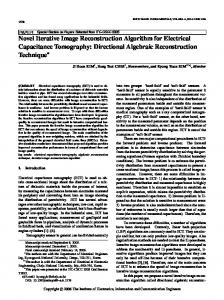
The numerical simulation for shape identification has been carried out for a 32 electrodes ERT in 3D, for a 14 electrodes ECT system in 2D and an 8 coils MIT system in 3D, is shown. The simulation data for image reconstruction generated by FEM software and in all cases an addition 2.5% Gaussian noise was added. Figure 1 shows the shape reconstruction in a numerical example. In three cases for ERT (figure 1. A), MIT (figure 1 B) and ECT (figure 1C), the shape identification of an inclusion object (in left) has been successfully done by monotonocity based algorithm. The forward model in ERT, EIDORS3D, was first order 3D nodal tetrahedral elements (Polydorides 2002), in MIT 3D first order edge FEM and with tetrahedral elements and in ECT 2D and using triangle elements. In MIT the trans impedance data was needed in multi frequency mode, in this numerical example we used 350Hz, 550Hz, 700Hz, 900Hz.

7

CONCLUSION

The monotonocity underlying resistance, capacitance and magnetic induction tomography potentially offers a fast, stable, non-iterative and non-linear reconstruction algorithm for two-phase mixtures. In this reconstruction technique there is no need for assumption of the smoothness on material properties; it is only required that (obviously) the material properties of the two phases are different.

8

ACKNOWLEDGEMENTS

This work was supported in part by Italian MIUR and EURATOM/ENEA/CREATE, and the UK EPSRC

237


(b)

(a)

(c) Figure 1: Shape identification, (a) ERT, left: desired shape, right: the solution, (b) MIT with 8 coils arranged radially in a plane, left: desired shape and right: the solution, (c ) ECT , left: the shape with inclusion , right: reconstructed shape

9

REFERENCES

GRIFFITHS H., (2001), Magnetic induction tomography, Meas. Sci. Technol vol.12, no.8, pp.11261131. PAULSON K., BRECKON W., PIDCOCK M., (1992), Electrode Modelling Impedance Tomography, Siam J. of Appl. Math., vol 52, no. 4, pp. 1012-1022.

in

Electrical

POLYDORIDES N., LIONHEART W.R.B., (2002), A Matlab toolkit for three-dimensional electrical impedance tomography: a contribution to the Electrical Impedance and Diffuse Optical Reconstruction Software project, Meas. Sci. Technol. 13 pp 1871-1883. SOMMERSALO E., CHENEY M., ISAACSON D., (1992), Existence and uniqueness for electrode models for electrical current computed tomography, Siam J. of Appl. Math., vol 52, no. 4, pp. 1023-1040. RUBINACCI G., TAMBURRINO A., VENTRE S., VILLONE F., (2002a), Shape identification in conductive materials by electrical resistance tomography, in E’NDE, Electromagnetic Non-destructive Evaluation (VI), F. Kojima et al. (Eds.), pp. 13-20, IOS Press. RUBINACCI G., TAMBURRINO A., VILLONE F., (2002b), Shape identification of conductive anomalies by a new ECT data inversion algorithm Proc. of the 4th International Conference Computation in Electromagnetics (CEM 2002), Bournemouth (UK).

RUBINACCI G., TAMBURRINO A., (2002c), A non-iterative ECT data inversion algorithm, Proc. of the 8th International Workshop on Electromagnetic Nondestructive Evaluation (ENDE 2002), June 2002, Saarbruecken, Germany. TAMBURRINO A., RUBINACCI G., (2002), A new non-iterative inversion method in electrical resistance tomography, Inverse Problems, vol. 18. YANG W.Q., PENG L.H., (2003), Image reconstruction algorithms for electrical capacitance tomography, Meas. Sci. Technol. (Review Article), 14, pp R1-R13.

238