{louis,georges,alan}@bic.mni.mcgill.ca http://www.bic.mni.mcgill.ca ... subjects, where sulcal misregistration is reduced by 20% (from 5.0mm to 4.0mm) and 11% ...
Non-linear Cerebral Registration with Sulcal Constraints D. Louis Collins, Georges Le Goualher, and Alan C. Evans McConnell Brain Imaging Centre, Montr´eal Neurological Institute, McGill University, Montr´eal, Canada {louis,georges,alan}@bic.mni.mcgill.ca http://www.bic.mni.mcgill.ca Abstract. In earlier work [1], we demonstrated that cortical registration could be improved on simulated data by using blurred, geometric, image-based features (Lvv ) or explicitly extracted and blurred sulcal traces on simulated data. Here, the technique is modified to incorporate sulcal ribbons in conjunction with a chamfer distance objective function to improve registration in real MRI data as well. Experiments with 10 simulated data sets demonstrate a 56% reduction in residual sulcal registration error (from 3.4 to 1.5mm, on average) when compared to automatic linear registration and an 28% improvement over our previously published non-linear technique (from 2.1 to 1.5mm). The simulation results are confirmed by experiments with real MRI data from young normal subjects, where sulcal misregistration is reduced by 20% (from 5.0mm to 4.0mm) and 11% (from 4.5 to 4.0mm) over the standard linear and nonlinear registration methods, respectively.
1
Introduction
In medical imaging processing research, correct automatic labelling of each voxel in a 3-D brain image remains an unsolved problem. Towards this goal, we have developed a program called animal (Automatic Nonlinear Image Matching and Anatomical Labelling) [2] which, like many other non-linear registration procedures, is based on the assumption that different brains are topologically equivalent and that non-linear deformations can be estimated and applied to one data set in order to bring it into correspondence with another. These non-linear deformations are then used (i) to estimate non-linear morphometric variability in a given population [3], (ii) to automatically segment MRI data [2], or (iii) to remove residual alignment errors when spatially averaging results among individuals. Our previous validation of animal showed that it worked well for deep structures [2], but sometimes had difficulty aligning sulci and gyri. In a follow-up paper presented at VBC96 [1], we described an extension of the basic non-linear registration method that used additional image-based features to help align the cortex. Simulations showed that Lvv -based features and blurred sulcal traces significantly improved cortical registration, however these results were not confirmed with real MRI data. In this paper, we demonstrate the use of automatically extracted and labelled sulci as extra features in conjunction with a chamfer W.M. Wells et al. (Eds.): MICCAI’98, LNCS 1496, pp. 974–984, 1998. c Springer-Verlag Berlin Heidelberg 1998
Non-linear Cerebral Registration with Sulcal Constraints
975
distance objective function [4,5]. Experimental results presented here (for both simulated and real data) show significant improvement over our previous work. In contrast to existing methods for cortical structure alignment that depend on manual intervention to identify corresponding points [6,7] or curves [8-12], the procedure presented here is completely automatic. While other 3D voxelbased non-linear registration procedures exist (e.g.,[12-20] none of these have looked specifically at the question of cortical features for cortical registration. The method presented here explicitly uses sulcal information in a manner similar to surface-matching algorithms described in [10,21,22] to improve cortical registration. However, our method is entirely voxel-based, completely automatic, and does not require any manual intervention for sulcal identification or labelling. The paper is organized as follows: Section 2 describes the brain-phantom used to create simulated data, the acquisition parameters for real MRI data, the non-linear registration method, and the features used in the matching process; Section 3 presents experiments on simulated MRI data with known deformations in order to compare our standard linear and non-linear registration procedures with the new technique and to determine a lower-bound for the registration error. Section 3 with experiments on 11 real MRI data sets, comparing the old and new registration methods. The paper concludes with a discussion and presents directions for further research.
2 2.1
Methods Input Data
Two sets of experiments are presented below where the first involves simulations to validate the algorithm and the second, real MRI data from normal subjects. Simulated Data: Simulations are required validate any image processing procedure since it is difficult, if not impossible to establish ground truth with in-vivo data. Here, we simulate MRI volumes [23] from different anatomies by warping a high resolution brain phantom [24] with a random (but known) deformation. Since both the deformation and structural information are known a priori, we can directly compute an objective measure of algorithm performance. Simulated MRIs: Magnetic resonance images are simulated by MRISIM [23], a program that predicts image contrast by computing NMR signal intensities from a discrete-event simulation based on the Bloch equations of a given pulse sequence. A realistic high-resolution brain phantom was used to map tissue intensities into MR images. The simulator accounts for the effects of various image acquisition parameters by incorporating partial volume averaging, measurement noise and intensity non-uniformity. The images in Fig. 1 were simulated using the same MR parameters as those described below (c.f., 2.1) for the real MRI acquisitions.
976
D.L. Collins, G. Le Goualher, and A.C. Evans
Simulated deformations: Most non-linear registration algorithms compute a continuous spatial mapping from the coordinate system of a given subject’s MRI to that of a target MRI volume. It is assumed that this mapping incorporates all morphological differences between subject and target anatomies. We turn this paradigm around to simulate different anatomies, based on a single target volume. Random spatial deformations were generated and applied to the brain phantom to build a family of homologous, but morphologically different brain phantoms. An MRI volume was simulated for each member of the family. Random spatial deformations were generated by defining a set of twenty landmarks within the target brain volume. A second deformed set of landmarks was produced by adding a random displacement to each of the landmark coordinates. Since previous work in our laboratory has shown anatomical variability to be on the order of 4-7mm [25], a Gaussian random number generator with a standard deviation of 5mm was used to produce each component of the displacement vector. The two resulting point sets (original and deformed) were then used to define a continuous 3-D thin-plate spline transformation function. Ten such deformations were generated and used to resample the original target data and produce 10 spatially warped source data sets for testing. The average deformation magnitude was 7.7mm with a maximum of 19.7mm. Figure 1 shows transverse slices (after linear stereotaxic registration) through the original and three of the ten warped volumes used in the experiments below. While these images demonstrate extreme deformations, they form a good test for animal.
Fig. 1. Simulated data This figure shows transverse slices at the level of the ventricles for four of the ten simulated test volumes, after resampling with the linear transformation recovered by animal. While these volumes are perhaps deformed more than one would find on average in the normal population, subjects representing an extreme of normal anatomical variability could be shaped like these examples. Note that while only 2-D images are shown in the figures, all calculations are computed in 3-D on volumetric data.
Non-linear Cerebral Registration with Sulcal Constraints
977
MRI Acquisition: In order to validate the animal algorithm with real data, eleven subjects were scanned on a Philips Gyroscan ACS 1.5 Tesla superconducting magnet system at the Montreal Neurological Institute using a T1-weighted 3-D spoiled gradient-echo acquisition with sagittal volume excitation (TR=18, TE=10, flip angle=30o , 1mm isotropic voxels, 140-180 sagittal slices). Without loss of generality, one of the 11 MRI volumes was chosen to serve as the target and the other 10 were registered to it. 2.2
Processing Pipeline
A number of processing steps are required to register two data sets together. We have combined preprocessing steps (image intensity non-uniformity correction [26], tube masking), linear registration (animal in linear mode [27]) and resampling into stereotaxic space, cortical surface extraction (msd [28,29]), tissue classification (insect [30]), automatic sulcal extraction (seal [31]) and non-linear registration (animal in nonlinear mode [2]) into a processing pipeline. After running this basic pipeline, a subject’s MRI volume can be visualized in stereotaxic space with its corresponding tissue labels, anatomical structure labels, cortical surface and sulcal ribbons — all in 3D. The following sections describe the registration and sulcal extraction procedures in more detail. Registration Algorithm: Registration is completed automatically in a two step process. The first [27] accounts for the linear part of the transformation by using correlation between Gaussian-blurred features (described below) extracted from both volumes. After automatic linear registration, there remains a residual non-linear component of spatial mis-registration among brains that is due (mostly) to normal anatomical morphometric variability. In the second step, the animal program estimates the 3D deformation field [2,3] required to account for this variability. The deformation field is built by sequentially stepping through the target volume in a 3D grid pattern. At each grid-node i, the deformation vector required to achieve local registration between the two volumes is found by optimization of 3 translational parameters (txi ,tyi ,tzi ) that maximize the objective function evaluated only in the neighbourhood region surrounding the node. The algorithm is applied iteratively in a multi-scale hierarchy, so that image blurring and grid size are reduced after each iteration, thus refining the fit. (The algorithm is described in detail in [2,32]). Features: The objective function maximized in the optimization procedure measures the similarity between features extracted from the source and target volumes. We use blurred image intensity and blurred image gradient magnitude, calculated by convolution of the original data with zeroth and first order 3D isotropic Gaussian derivatives in order to maintain linearity, shift-invariance and rotational-invariance in the detection of features. Since both linear and nonlinear registration procedures are computed in a multi-scale fashion, the original
978
D.L. Collins, G. Le Goualher, and A.C. Evans
MR data was blurred at two different scales: fwhm=8, and 4mm, with the fwhm= (2.35σ) of the Gaussian kernel acting as a measure of spatial scale. The enhanced version of animal uses geometrical landmarks such as sulci to improve cortical alignment. We have previously detailed a method called seal (Sulcal Extraction and Automatic Labeling) to automatically extract cortical sulci (defined by the 2D surface extending from the sulcal trace at the cortical surface to the depth of the sulcal fundus) from 3D MRI [33,31]. Each sulcus is extracted in a two step process using an active model similar to a 2D Snake that we call an active ribbon. First, the superficial cortical trace of the sulcus is modeled by a 1D snake-spline [34], that is initialized to loci of negative curvature of the cortical surface. Second, this snake is then submitted to a set of forces derived from (1) tissue classification results, (2) differential characteristics of the image intensities near the cortex and (3) a distance-from-cortex term to force the snake to converge to the sulcal fundus. The set of successive iterative positions of the 1D snake define the sulcal axis. These loci are then used to drive a 2D active ribbon which forms the final representation of the sulcus. When applied to an MRI brain volume, the output of this automatic process consists of a set of Elementary Sulcal Surfaces (ESS) that represent all cortical sulcal folds. A number of these ESSs may be needed to represent a sulcus as defined by an anatomist. Simply blurring the voxel masks that represent the sulci at scales of fwhm=16 and 8mm so that they could be directly incorporated into the standard animal procedure for correlative matching was found not to improve cortical registration for real MRI data [1]. Here, in order to incorporate the geometric sulcal information represented by the ESS, the sulcal ribbons are voxelated. Like Sandor et. al.[10], we use a chamfer distance function to drive sulci together. This methods brings sulci that are initially far apart into registration. 2.3
Error Measures
In order to quantitatively evaluate the methods and compare them with previously published results [1], a 3D root-mean-squared (rms) minimum distance measure, Dsurf , was computed for the ESS of selected sulci1 that were identified manually by a medically-trained expert on the phantom volumes and on the real MRI volumes. The 3D rms minimum distance measure is defined on a point-wise basis, computing the root mean square (over all nodes in the ESS defining the 1
The following 16 sulci were traced bilaterally using a visualization tool that shows a 3D surface rendering of the cortex and orthogonal slices through the brain volume: (a) central sulcus and (b) the Sylvian fissure; (c) the superior, (d) the middle, and (e) the inferior frontal sulci; (f) the vertical (a.k.a. ascending) and (g) the horizontal rami of the Sylvian fissure, as well as (h) the incisura (located between these other two rami); (i) the olfactory sulcus as well as (j) the sulcus lateralis, (k) the sulcus medialis, (l) the sulcus intermedius, and (m) the sulcus transversus (all found along the orbitofrontal surface of the brain); (n) the precentral and (o) the postcentral sulci; and finally (p) the intraparietal sulcus.
Non-linear Cerebral Registration with Sulcal Constraints
979
sulcus) of the minimum distance between each node in the transformed source sulcus and closest point on the target sulcus surface.
3
Experiments and Results
Two series of three experiments were completed varying only the features used by animal where the first series was completed for simulated data, and the second series, for real MRI data. In each experiment, 10 MRI volumes were registered to the chosen target volume. The 3 different experiments were defined as follows: (1) animal in standard non-linear mode, (2) animal+selected sulci, (3) animal+all sulci after using selected sulci. In method 2, the problem of establishing correspondence is addressed by using ten extracted sulci (superior and middle frontal, Sylvian, olfactory and central, on both hemispheres) as features in addition to the blurred MRI intensity volume already used by animal, The third method is an attempt to improve the second, by adding all sulci automatically extracted by seal into the registration process after completing the animal+selected sulci registration. A linear transformation is also presented for comparisons. Figures 2 and 3 summarize the results qualitatively for simulated and real data, respectively. Tables 1 and 2 present quantitative results for the measure described above. TABLE 1 lin Central 3.2;1.5 Postcentral 4.2;2.3 Middle Frontal 3.2;1.0 Superior Frontal 3.4;1.9 Sylvian 4.0;1.3 Olfactory 3.2;4.2 average (n=16) 3.4;2.3
simulations ∇ ∇+5 1.2;1.4 0.7;0.3 2.2;2.4 1.3;1.5 1.4;1.2 0.7;0.6 1.8;2.1 1.6;2.1 3.0;1.2 2.4;0.9 1.7;2.8 1.5;2.9 2.1;2.1 1.6;1.7
TABLE 2 ∇ + all 0.7;0.4 1.3;1.5 0.7;0.6 1.7;2.1 2.4;1.0 1.6;2.8 1.5;1.7
lin 4.7;1.3 6.4;1.7 6.2;3.5 6.2;3.8 5.2;1.6 2.1;1.7 5.0;3.2
real ∇ 4.1;1.4 6.1;2.0 5.4;3.2 5.6;3.6 5.0;1.4 1.6;1.9 4.5;3.1
MRI ∇+5 2.5;1.2 5.0;1.7 4.5;3.1 4.4;3.9 3.6;0.9 1.3;1.6 4.0;3.1
∇ + all 2.5;1.2 5.0;1.8 4.7;3.2 4.4;4.0 3.7;1.0 1.4;1.8 4.0;3.1
Quantitative results for simulations and real data. Mean and standard deviation of Dsurf minimum distance results (mean(Dsurf );std(Dsurf )) for linear (lin), ANIMAL (∇), ANIMAL+selected sulci (∇+5), ANIMAL with all sulci (∇+all) registration methods. Average is computed for both left and right hemispheres for 16 sulci on 10 subjects. All measures in millimeters.
3.1
Simulations
Standard ANIMAL: In the first experiment (Fig. 2-b) we can see that the global brain shape is properly corrected and that the main lobes are mostly aligned since the central and Sylvian sulci are better aligned than in the linear registration. Even though previous experiments in [2] have shown that basal ganglia structures (e.g., thalamus, caudate, putamen, globus pallidus) and ventricular structures are well registered (with overlaps on the order of 85% to 90%) for both simulated and real data, the simulations presented here indicate that the
980
D.L. Collins, G. Le Goualher, and A.C. Evans
standard animal technique cannot always register cortical structures by using only blurred image intensities and gradient magnitude features. ANIMAL+selected sulci: In Fig. 2-c, 10 extracted sulci (superior and middle frontal, Sylvian, olfactory and central, on both hemispheres) were used as additional features in animal to address problems in establishing correspondence. Visual inspection of Fig. 2-c shows that the previous misalignments in the motorsensory area have been corrected, and alignment for neighbouring structures has improved greatly. Indeed, when evaluated on the central sulcus, the Dsurf measure improves dramatically: 3.2mm for linear; 2.0mm for standard non-linear; 0.7mm for animal with labelled sulci. The standard deviation of Dsurf decreases as well, indicating tighter grouping around the target sulci. The 0.54mm average Dsurf reduction is highly significant (p < 0.0001, T = 157, d.o.f. = 320, paired T -test over all sulci and all subjects). ANIMAL+selected sulci+all sulci: In this experiment, the animal+selected sulci transformation is used as input where all sulci extracted by seal are used as features in an attempt to further improve cortical alignment in regions that are not close to the previously selected sulci. The improvement is evident qualitatively in Fig. 2-d and quantitatively in Table 1 where the average Dsurf , evaluated over all sulci and all subjects drops from 1.6mm for the standard animal to 1.5mm when using all sulci. While this improvement is small, it is statistically significant (p < 0.0001, T = 88.5, d.o.f. = 320, paired T -test). 3.2
Real MRI Data
Standard ANIMAL: When applied to real data, the image in Fig. 3-b shows that that the standard animal non-linear registration is not enough to align cortical structures. In fact, it does not appear to be much better than the linear registration. This is confirmed by the quantitative results in Table 2, where the average Dsurf value for the standard animal registrations is only slightly better than that for linear registrations. ANIMAL+selected sulci: The use of 5 paired sulci improves cortical registration significantly in the neighbourhood of the chosen sulci as shown in Fig. 3c. The central sulcus (purple), superior frontal (orange), middle frontal (red), olfactory (black) and Sylvian (red) (arrows) are well defined, and this is confirmed by improved Dsurf values in Table 2, when compared to the standard animal registrations. Unfortunately, the effect appears to be relatively local in that alignment of neighbouring sulci are only somewhat improved (e.g., postcentral sulcus). This is probably because there is no explicit representation of the other sulci in the registration, so they do not participate in the fitting process. However, using some labelled sulci yields a 0.50mm average Dsurf reduction (from 4.5 to 4.0mm) that is highly significant (p < 0.0001, T = 157, d.o.f. = 320, paired T -test). ANIMAL+selected sulci+all sulci: When the previous result is used as input for a registration using all sulci as features, then some of the other sulci (e.g., postcentral) come into alignment, however others may be attracted to non-homologous sulci, since no explicit labelling of sulci is used in this step.
Non-linear Cerebral Registration with Sulcal Constraints
4
981
Discussion and Conclusion
The simulation results indicate clearly that the registrations computed by animal improve substantially when using the extra cortical features. The random deformations used to simulate different anatomies (section 2.1) only model one aspect of anatomical variability, namely the second-order morphological difference between subjects (i.e., a difference in position for a given structure after mapping into a standardized space). The simulations do not account for different topologies of gyral and sulcal patterns. For example, it cannot change the region corresponding to Heschl’s gyrus, to contain double gyri when the phantom has only a single. Still, the value of these simulations is not diminished since they can be used to determine a lower-bound on the registration error — corresponding to the optimal case when a 1-to-1 mapping exists between two subjects. The experiments with real data indicate that the use of automatically extracted and labelled sulci in conjunction with a chamfer distance function can significantly improve cortical registration. One must keep in mind that the Dsurf measure includes possible sulcal mis-identification and sulcal extraction errors (from seal) in addition to animal’s mis-registration error. We are working on quantifying the performance of seal in order to improve the error measure. Further improvements to the registration algorithm will require a slight change in fitting strategy to account for different cortical topologies apparent in real MRI data. We envision using a number of different targets simultaneously, where each target will account for a particular type of sulcal pattern [35]. The current version of animal now allows the use of a chamfer-distance objective function to align sulci, however nothing in the implementation is sulcispecific. Indeed, any geometric structure that can be voxelated can be incorporated into the matching procedure to further refine the fit. We are currently evaluating the incorporation of explicitly extracted cortical surfaces [28,29] into the registration process. Acknowledgments: The authors would like to express their appreciation for support from the Human Frontier Science Project Organization, the Canadian Medical Research Council (SP-30), the McDonnell-Pew Cognitive Neuroscience Center Program, the U.S. Human Brain Map Project (HBMP), NIMH and NIDA. This work forms part of a continuing project of the HBMP-funded International Consortium for Brain Mapping (ICBM) to develop a probabilistic atlas of human neuroanatomy. We also wish to acknowledge the manual labelling of sulcal traces completed by Rahgu Venegopal.
References 1. D. Collins, G. LeGoualher, R. Venugopal, Z. Caramanos, A. Evans, and C. Barillot, “Cortical constraints for non-linear cortical registration,” in Visualization in Biomedical Computing (K. H¨ oene, ed.), (Hamburg), pp. 307–316, Sept 1996. 2. D. Collins, C. Holmes, T. Peters, and A. Evans, “Automatic 3D model-based neuroanatomical segmentation,” Human Brain Mapping, vol. 3, no. 3, pp. 190–208, 1995.
982
D.L. Collins, G. Le Goualher, and A.C. Evans
3. D. L. Collins, T. M. Peters, and A. C. Evans, “An automated 3D non-linear image deformation procedure for determination of gross morphometric variability in human brain,” in Proceedings of Conference on Visualization in Biomedical Computing, SPIE, 1994. 4. G. Borgefors, “Distance transformations in arbitrary dimensions,” Computer Graphics, Vision and Image Processing, vol. 27, pp. 321–345, 1984. 5. G. Borgefors, “On digital distance transforms in three dimensions,” Computer Vision Image Understanding, vol. 64, pp. 368–76, 1996. 6. A. C. Evans, W. Dai, D. L. Collins, P. Neelin, and T. Marrett, “Warping of a computerized 3-D atlas to match brain image volumes for quantitative neuroanatomical and functional analysis,” in Proceedings of the International Society of Optical Engineering: Medical Imaging V, vol. 1445, (San Jose, California), SPIE, 27 February – 1 March 1991. 7. F. Bookstein, “Thin-plate splines and the atlas problem for biomedical images,” in Information Processing in Medical Imaging (A. Colchester and D. Hawkes, eds.), vol. 511 of Lecture Notes in Computer Science, (Wye, UK), pp. 326–342, IPMI, Springer-Verlag, July 1991. 8. Y. Ge, J. Fitzpatrick, R. Kessler, and R. Margolin, “Intersubject brain image registration using both cortical and subcortical landmarks,” in Proceedings of SPIE Medical Imaging, vol. 2434, pp. 81–95, SPIE, 1995. 9. S. Luo and A. Evans, “Matching sulci in 3d space using force-based deformation,” tech. rep., McConnell Brain Imaging Centre, Montreal Neurological Institute, McGill University, Montreal, Nov 1994. 10. S. Sandor and R. Leahy, “Towards automated labelling of the cerebral cortex using a deformable atlas,” in Information Processing in Medical Imaging (Y. Bizais, C. Barillot, and R. DiPaola, eds.), (Brest, France), pp. 127–138, IPMI, Kluwer, Aug 1995. 11. D. Dean, P. Buckley, F. Bookstein, J. Kamath, and D. Kwon, “Three dimensional mr-based morphometric comparison of schizophrenic and normal cerebral ventricles,” in Proceedings of Conference on Visualization in Biomedical Computing, Lecture Notes in Computer Science, p. this volume, Springer-Verlag, Sept. 1996. 12. R. Bajcsy and S. Kovacic, “Multiresolution elastic matching,” Computer Vision, Graphics, and Image Processing, vol. 46, pp. 1–21, 1989. 13. R. Dann, J. Hoford, S. Kovacic, M. Reivich, and R. Bajcsy, “Three-dimensional computerized brain atlas for elastic matching: Creation and initial evaluation,” in Medical Imaging II, (Newport Beach, Calif.), pp. 600–608, SPIE, Feb. 1988. 14. M. Miller, Y. A. G.E. Christensen, and U. Grenander, “Mathematical textbook of deformable neuroanatomies,” Proceedings of the National Academy of Sciences, vol. 90, no. 24, pp. 11944–11948, 1990. 15. J. Zhengping and P. H. Mowforth, “Mapping between MR brain images and a voxel model,” Med Inf (Lond), vol. 16, pp. 183–93, Apr-Jun 1991. 16. K. Friston, C. Frith, P. Liddle, and R. Frackowiak, “Plastic transformation of PET images,” Journal of Computer Assisted Tomography, vol. 15, no. 1, pp. 634–639, 1991. 17. G. Christensen, R. Rabbitt, and M. Miller, “3D brain mapping using a deformable neuroanatomy,” Physics in Med and Biol, vol. 39, pp. 609–618, 1994. 18. J. Gee, L. LeBriquer, and C. Barillot, “Probabilistic matching of brain images,” in Information Processing in Medical Imaging (Y. Bizais and C. Barillot, eds.), (Ile Berder, France), IPMI, Kluwer, July 1995.
Non-linear Cerebral Registration with Sulcal Constraints
983
19. J. Gee, “Probabilistic matching of deformed images,” Tech. Rep. Technical report MS-CIS-96, Department of Computer and Information Science, University of Pennsylvania, Philadelphia, 1996. 20. G. Christensen, R. Rabbitt, and M. Miller, “Deformable templates using large deformation kinematics,” IEEE Transactions on Image Processing, 1996. 21. P. Thompson and A. Toga, “A surface-based technique for warping 3-dimensional images of the brain,” IEEE Transactions on Medical Imaging, vol. 15, no. 4, pp. 383–392, 1996. 22. C. Davatzikos, “Spatial normalization of 3d brain images using deformable models,” J Comput Assist Tomogr, vol. 20, pp. 656–65, Jul-Aug 1996. 23. R. Kwan, A. C. Evans, and G. B. Pike, “An extensible MRI simulator for postprocessing evaluation,” in Proceedings of the 4th International Conference on Visualization in Biomedical Computing, VBC ‘96:, (Hamburg), pp. 135–140, September 1996. 24. D. Collins, A. Zijdenbos, V. Kollokian, J. Sled, N. Kabani, C. Holmes, and A. Evans, “Design and construction of a realistic digital brain phantom,” IEEE Transactions on Medical Imaging, 1997. submitted. 25. C. Sorli´e, D. L. Collins, K. J. Worsley, and A. C. Evans, “An anatomical variability study based on landmarks,” tech. rep., McConnell Brain Imaging Centre, Montreal Neurological Institute, McGill University, Montreal, Sept 1994. 26. J. G. Sled, A. P. Zijdenbos, and A. C. Evans, “A non-parametric method for automatic correction of intensity non-uniformity in MRI data,” IEEE Transactions on Medical Imaging, vol. 17, Feb. 1998. 27. D. L. Collins, P. Neelin, T. M. Peters, and A. C. Evans, “Automatic 3D intersubject registration of MR volumetric data in standardized talairach space,” Journal of Computer Assisted Tomography, vol. 18, pp. 192–205, March/April 1994. 28. D. MacDonald, D. Avis, and A. C. Evans, “Multiple surface identification and matching in magnetic resonance images,” in Proceedings of Conference on Visualization in Biomedical Computing, SPIE, 1994. 29. D. MacDonald, Identifying geometrically simple surfaces from three dimensional data. PhD thesis, McGill University, Montreal, Canada, December 1994. 30. A. P. Zijdenbos, A. C. Evans, F. Riahi, J. Sled, J. Chui, and V. Kollokian, “Automatic quantification of multiple sclerosis lesion volume using stereotaxic space,” in Proceedings of the 4th International Conference on Visualization in Biomedical Computing, VBC ‘96:, (Hamburg), pp. 439–448, September 1996. 31. G. L. Goualher, C. Barillot, and Y. Bizais, “Three-dimensional segmentation and representation of cortical sulci using active ribbons,” in International Journal of Pattern Recognition and Artificial Intelligence, 11(8):1295-1315 1997. 32. D. Collins and A. Evans, “Animal: validation and applications of non-linear registration-based segmentation,” International Journal and Pattern Recognition and Artificial Intelligence, vol. 11, pp. 1271–1294, Dec 1997. 33. G. L. Goualher, C. Barillot, Y. Bizais, and J.-M. Scarabin, “Three-dimensional segmentation of cortical sulci using active models,” in SPIE Medical Imaging, vol. 2710, (Newport-Beach, Calif.), pp. 254–263, SPIE, 1996. 34. F. Leitner, I. Marque, S. Lavalee, and P. Cinquin, “Dynamic segmentation: finding the edge with snake splines,” in Int. Conf. on Curves and Surfaces, pp. 279–284, Academic Press, June 1991. 35. M. Ono, S. Kubik, and C. Abernathey, Atlas of Cerebral Sulci. Stuttgart: Georg Thieme Verlag, 1990.
984
D.L. Collins, G. Le Goualher, and A.C. Evans central post−central intraparietal
pre−central
sup frontal inf frontal mid frontal
lateralis intermedias medialis
a−linear
olfactory
c−ANIMAL+5sulci
Sylvian ascending incisura horizontal transversus
b−ANIMAL
d−ANIMAL+all sulci
Fig. 2. Simulations: ANIMAL-only vs ANIMAL+sulci Left-side view of the cortical traces of 16 sulci from 10 simulated volumes overlaid on an average cortical surface after mapping into stereotaxic space with the different transformations indicated. These simulations show that extracted and labelled sulci improve the standard animal registrations.
central post−central intraparietal
pre−central
sup frontal inf frontal mid frontal
lateralis intermedias medialis
a−linear
c−ANIMAL+5sulci
olfactory
Sylvian ascending incisura horizontal transversus
b−ANIMAL
d−ANIMAL+all sulci
Fig. 3. Real data: ANIMAL-only vs ANIMAL+sulci Left-side view of the cortical traces of 16 sulci from 10 real subjects overlaid on an average cortical surface after mapping into stereotaxic space. It is easy to see that the standard registration technique does not deal well with cortical structures, however addition sulcal constraints improve cortical registration significantly for real data near sulci participating in the registration process (arrows).