Non-Linear Graph-Based Codes for Source Coding - UPCommons

2009 IEEE Information Theory Workshop

Non-Linear Graph-Based Codes for Source Coding David Matas1 , Meritxell Lamarca1,2, and Javier Garcia-Frias2 1

Signal Theory and Communications Department, Technical University of Catalonia Email: (dmatas, xell)@gps.tsc.upc.edu 2 Department of Electrical and Computer Engineering, University of Delaware Email: (lamarca, jgarcia)@ee.udel.edu

Abstract—We introduce a new family of graph-based source codes that can be regarded as a nonlinear generalization of LDPC codes, and apply them to the compression of asymmetric binary memoryless sources. Simulation results and the application of density evolution show that the proposed family presents a performance very close to the theoretical limits, clearly outperforming schemes based on linear codes.

I. I NTRODUCTION Nonlinear source codes are potentially more powerful than linear ones, since they include the latter as a particular case. The fact that non-linear codes may have different distance properties for different codewords can be exploited to guarantee better distance profiles for the most likely information sequences, whereas linear codes always possess identical distances profiles for all codewords. In spite of this potential advantage, there has been relatively little work in the literature on non-linear codes, since linear codes are known to be asymptotically optimum for infinite codeword length. In this paper we introduce a new family of non-linear binary codes based on graphs. The proposed scheme can be seen as a non-linear generalization of LDPC codes, which includes them as a particular case while maintaining many of the desirable features of LDPC codes. Namely, i) the proposed non-linear codes can be graphically represented by means of a factor graph, ii) they can be decoded using belief propagation, and iii) their performance can be predicted using density evolution (DE), and thus they can be easily designed when long codewords are considered. The proposed codes are aimed at efficiently compressing asymmetric binary memoryless sources (i.e., at a given time the source generates a 0 (1) with probability p(0) (p(1) = 1 − p(0)). Obviously, the number of 0s and 1s will be unbalanced for the most likely information sequences, so it makes sense to employ a source code that provides different distance properties for information sequences that have different number of 0s. As we will see in the sequel, this can be easily done by using the proposed non-linear code structure. In addition, the proposed architecture provides a natural way to map unbalanced input sequences into compressed sequences with similar number of 0s and 1s, which is known to be one of the features of a good source code. This work has been partially funded by the Spanish Science and Technology Commissions and by FEDER funds from the European Commission: TEC2007-68094-C02-02, CSD2008-00010.

978-1-4244-4983-5/09/$25.00 © 2009 IEEE

The duality between source coding and channel coding has been exploited in the literature to propose the use of turbo and LDPC codes for lossless [1], [2] and lossy source coding [3], [4], as well as for joint source-channel coding [5], [6], [7], [8]. The application of these codes to compression of correlated sources has been particularly successful [9], [10]. The use of non-linear codes for lossless and lossy compression has been recently proposed in the literature [11], [12], but most of this work focuses on codes that are difficult to analyze and generalize. Differently, for any given compression rate the family of non-linear codes proposed here can be easily analyzed and optimized by applying density evolution [13]. II. S YSTEM

SET- UP

We consider the problem of almost lossless source coding of an asymmetric memoryless binary source with p(1) > p(0), but it is worth mentioning that the dual case, p(0) > p(1), can be easily studied by either inverting the source or by replacing the AND operators used in the sequel by OR operators. We consider fixed-length block source codes, where a sequence of K information bits, b1 b2 . . . bK , is compressed into a codeword of N < K bits, so that a code with compression rate R = N/K is obtained. III. L OW- DENSITY PRODUCT

CHECK

(LDP R C)

CODES

A. Code definition We first introduce a novel family of non-linear codes that results when each coded bit, pj , is obtained as the product (AND) of a few information bits bi . Thus, we generate a codeword of length N as Y pj = bi , j = 1 . . . N, i∈Sj

where Sj is the set of dpj indices (1 ≤ dpj ≤ K) that defines which information bits are used to generate pj . Note that this is a nonlinear code, due to the use of the AND binary operator. The ability of this code to compress sources with p(1) > p(0) is clear. In this case, a good source code should map a sequence with more 1s than 0s into a shorter one where the number of 1s and 0s is more balanced (ideally the same). It must also do so in a manner that allows the recovery of the original sequence. Since pj = 1 if and only if bi = 1 ∀i ∈ Sj , the AND operation applied to dpj inputs has the capability of compressing dpj 1s into a single 1. Notice that when p(1) > p(0), the AND operator also has the desired property

318

x

of increasing the number of 0s in the codeword: it yields a 1 at the output with probability p(1)dpj < p(1). The encoding process can be described in a compact form by defining a K × N matrix P whose (i, j) entry is 1 if the information bit bi is employed in the computation of the coded bit pj , and 0 otherwise. Using this compact notation, we will represent the encoding process as p = b  P, p = [p1 . . . pN ] , b = [b1 . . . bK ] .

(1)

apriori source information

Hence, matrix P fully characterizes the code, which can be represented by a factor graph as depicted in Fig. 1. Compared to the graph of an LDPC code, the only difference is that the check nodes have been replaced by product nodes.

b1

=

p1

. . .

=

P

=

. . bK .

. . .

. . .p =

N

=

information bits

Figure 1.

product nodes

coded bits

Factor graph of the proposed LDPrC codes.

Following the same convention as in other graph-based codes, we will say that dpj is the degree of the product node associated to pj , and we will also denote the number of products where an information bit bi participates as the degree L of the corresponding bit node dN bi . If all bit and product nodes L NL have the same degree, dpj = dp ∀j and dN ∀i, we bi = db will say that the LDPrC code is regular, and its compression L rate is N/K = dN b /dp . B. Decoding The proposed codes are constructed using a sparse P. Hence, if the codeword is long enough and the matrix has been properly designed, there will be few cycles in the graph and belief propagation will provide a quite accurate approximation of maximum-a-posteriori decoding. The message passing equations for the variable nodes will be the same as in LDPC codes, whereas new equations must be derived for the product nodes. To derive the message passing equations in a product node, consider the case of a two-input AND operator z = xy depicted in Fig. 2. As represented in the figure, let us denote by L×→v and Lv→× the LLR messages that go from the product node × to variable node v (being v either z, x or y) and p(v=1) . Then, we can write viceversa, where LLR(v) = log p(v=0) the decoding equations for this product node of degree two as   1 + 2eLx→× +Lz→× L×→y = log (2) 1 + 2eLx→×
L×→z = Lx→× + Ly→× − log 1 + eLx→× + eLy→× (3)

For product nodes of higher degree, the messages can be computed recursively from the expressions above.

Lx→× L×→z

L×→x L×→y

y Figure 2.

z Lz→× Ly→×

LLR messages exchanged in a product node.

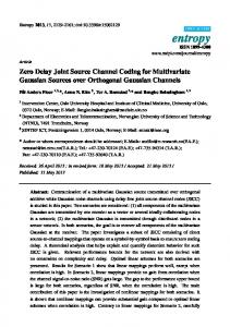
Notice that the behavior of product nodes is very different from that of a check node in standard LDPC codes, and the LLRs propagate in a very different manner: Whereas in standard LDPC codes infinite reliability in all edges results in infinitely reliable outgoing messages, this does not happen in product nodes. Indeed, for the previous product with two inputs, • If Lz→× = +∞ then L×→y = +∞ irrespective of the value of Lx→× . • If Lz→× = −∞ and Lx→× = −∞, then L×→y = 0. In Q other words, knowledge that a certain product node pj = i∈Sj bi is 1 immediately provides perfect knowledge of all information bits that participate in the product (all operands must be 1). In addition, if a certain product node is 0 and one of the operands is also known to be 0, then no information on the remaining operands can be derived from this node. As illustrated in Section III-D, this feature leads to error floors and limits the performance of LDPrC codes. C. Code performance analysis We expect the concentration theorem to apply for LDPrC codes. Thus, if edges between the different node layers are randomly set, and provided that the codeword is long enough, the code performance should only depend on the degree profile of each node type. Hence, density evolution should be able to predict the code performance. Note, however, that the standard DE procedure must be modified to take into account the fact that now, due to the code non-linearity, the performance depends on the information message, and thus it is not enough to just consider the all-zero message. In our analysis, we assume that the performance only depends on the message weight and on the code degree profile. This results in a code design in which we optimize the performance for the asymmetric source (i.e., typical sequence with p(0)K 0’s and (1 − p(0))K 1’s when K → ∞). As we will see in the following section, the DE equations, which are presented in the appendix, accurately predict the code performance. This is a major difference with respect to previously proposed non-linear codes in the literature: to the best of our knowledge, no non-linear code has been proposed whose analysis and design with nearly optimum decoding can be predicted systematically. D. Simulation results Fig. 3 depicts the bit error rate (BER) performance as a function of the source entropy for regular LDPrC codes with L compression rate 12 , K = 200000 and degrees (dN b , dp ) of (2,4), (3,6) and (4,8), and compares it with that of regular LDPC codes with the same degrees and length. Both DE

319

LDPC parity checks. Using the same compact notation as in Section III, we have p = b  P, p = [p1 . . . pαN ] , b = [b1 . . . bK ]   c = bG, c = c1 . . . c(1−α)N , b = [b1 . . . bK ] ,

=

. . . dL bi

=

G

dcj

. . .

=

=

=

=

. . . = L dN bi

P

. . . dpj

=

αN

. . . =

information bits

−2

Figure 4.

p(0) nonlinear (2,4) MC nonlinear (2,4) DE nonlinear (3,6) MC nonlinear (3,6)DE nonlinear (4,8) MC nonlinear (4,8) DE linear (2,4) MC linear (2,4) DE linear (3,6) MC linear (3,6) DE linear (4,8) MC linear (4,8) DE

10

BER

(1 − α)N

. . .

0

−4

10

−6

10

0.25

0.3

0.35

0.4 0.45 0.5 Source entropy (bits)

0.55

0.6

0.65

product nodes

coded bits

Factor graph of the proposed LDPC-LDPrC codes.

B. Decoding and code performance analysis

−8

0.2

(5)

check nodes

10

10

(4)

where G is the sparse matrix that characterizes the LDPC code and the codeword is then built as [p c]. Therefore, matrices G and P fully characterize the hybrid LDPC-LDPrC code. Fig. 4 depicts the factor graph of the new code, which now includes bit, product, and parity-check nodes. Note that the information NL bit nodes have now two degrees dL bi and dbi , corresponding to the linear and non-linear code parts, respectively.

apriori source information

analysis and Montecarlo (MC) simulations after 50 iterations are plotted. For comparison purposes, the value p(0) corresponding to the source entropy under consideration is also depicted, since this would be the error probability if the decoder did not converge and decisions on the information bits were made based on the a priori source information (since p(1) > p(0), all bits would be assumed to be 1 so that BER = p(0)). Note that in all cases DE accurately predicts the code performance. Two aspects are worth mentioning. First, curves for LDPrC codes always have very small slope. This is due to the specific behavior of AND nodes indicated in Section III-B, which causes a structural error floor that is independent of the codeword length. For instance, consider an information L bit, bi , connected to dN product nodes. If each of these bi product nodes is connected to at least one information bit taking value 0 (excluding bi ), then the value of bi cannot be recovered. Hence, if bi = 0 an error will be made at the decoder (since the decision would be based purely on the a priori information and p(1) > p(0)). This could be a drawback for these codes, but the curves show a very interesting second aspect: the BER for source entropies close to or even greater than the code compression rate of 12 are well below p(0) and easily outperform linear codes. This is a distinctive feature of LDPrC codes, which can be exploited to design more complex structures, such as those described in Section IV, with excellent convergence thresholds.

0.7

Figure 3. BER vs source entropy for LDPrC codes. Linear LDPC codes of the same rate and degrees are also depicted. MC simulations and DE results are compared.

IV. H YBRID LDPC-LDP R C CODES

LDPC-LDPrC codes are designed using sparse matrices G and P. Thus, if the codeword is long enough, belief propagation will provide an accurate approximation of maximum-aposteriori decoding. As in the case of LDPrC codes, LDPC-LDPrC codes can be analyzed using a modified version of density evolution. The appendix provides the DE analysis of the hybrid LDPC-LDPrC codes (and also of LDPrC codes, as those are obtained setting α = 1). As evidenced in the simulation results presented in the following section, code performance is accurately predicted by DE, which can thus be used as an efficient tool for the design of LDPC-LDPrC codes that approach the theoretical limits.

A. Code definition

C. Simulation results

The structural error floor of LDPrC codes can be substantially reduced if the information bit nodes are also connected to some parity check nodes that allow to recover the bits that can not be retrieved from product nodes. Hence, in this section we consider the parallel concatenation of a non-linear LDPrC code with a high rate linear LDPC code aimed at correcting the error floor at the output of the non-linear code. We consider the case where a fraction α of coded bits is generated following equation (1) and the reminder fraction, 1 − α, are standard

We focus our attention into a very simple case of the generic architecture proposed in Section IV-A that can be described with very few parameters. Specifically, we consider the case where the degree of the information bit nodes is regular, dL b L and dN for the LDPC and the LDPrC codes, respectively. b Then, for a given code rate r = N/K and parameter α, the average degree of the product and the check nodes must be L L equal to dp = dN b /rα, dc = db /r(1 − α). Since these may result to be fractional, we will set the products/checks to have

320

degrees equal to the closest lower and upper integers. Note that these codes are totally characterized by the set of parameters L L (N, K, dN b , db , α). Fig. 5 depicts the performance of the regular LDPC-LDPrC L with compression rate 12 , α = 0.7, dN = 3 and dL b b = 2, and compares it with the best regular LDPC code with the same rate (the (3,6) code). The performance for MC simulations and DE analysis is depicted for 1,5,10, 20 and 100 decoder iterations, using in the case of MC a codeword of length K = 200000. It is remarkable that DE analysis and MC simulations match very well. The difference between them for low BER values can be attributed to the presence of cycles in the graph and to the finite codeword length. Notice that the LDPrC code clearly outperforms the linear LDPC code. Fig. 6 depicts the performance of several LDPC-LDPrC codes, with K = 200000, compression rate 12 and diverse L values of α, dN and dL b b . Note that all of them outperform the linear regular (3,6) LDPC code. Since the performance of LDPC codes improves when irregular degree profiles are employed, we also expect performance gains by using irregular degrees in LDPC-LDPrC codes, thanks to the degrees of freedom introduced by the non-linear product stage and their good BER properties for high entropies.

check node. Similarly, denote as {pn→pd }n=0,1 the pdf of the message sent to a product node from a bit node whose corresponding information bit is n. Then, assuming these pdfs to be known (we will explain later in section VI.C how to compute them), we can compute the pdf for the message arriving to an information bit node after the decoder has updated the check node and the product node messages using the equations described next in sections VI.A and VI.B. A. Check nodes The message passed from a check node of degree d to an information bit node is computed as a function of the messages coming from the other d − 1 information bit nodes and the value of the coded bit. Let us denote the pdf of this message when l out of the d − 1 information bits are equal to 0 (and d − 1 − l to 1) and the coded bit associated to this check node (l,d) has value o as {po,ck }o=0,1 . This pdf can be computed as a function of {pn→ck }n=0,1 using the LLR update equation for the check nodes and the procedure indicated in [14]. The pdf of the message arriving at an information bit node after the check node updating can be computed taking into (l,d) account all individual pdfs {po,ck }o=0,1 and their probability of occurrence. This pdf is given by the following equations, depending on whether the information bit node is 0 or 11 :

V. C ONCLUSION We have proposed a very promising family of non-linear source codes that generalizes LDPC codes by incorporating AND nodes into the factor graph. Simulation results confirm that the resulting performance is much better than that of linear codes, and very close to the theoretical limits. The behavior of the proposed structure can be accurately predicted using an extension of density evolution. Thus, we expect to be able to apply density evolution to design even better LDPCLDPrC codes by incorporating irregular degree profiles and stage concatenation. VI. A PPENDIX : D ENSITY

EVOLUTION

The equations for the DE analysis must be modified to take into account the transmission of a codeword other than the all-zero sequence. In the sequel, we summarize the equations that must be used to model the probability density function (pdf) of the messages exchanged between information bit nodes and check and product nodes depending on whether the corresponding bit node is 0 or 1. Let us first define {λi }i=1,...,Dp , {βi }i=1,...,Dc , {γi }i=1,...,DbN L , {δj }j=1,...,DbL } as the fraction of edges that belong respectively to a degree-i product node, degree-i check node, and the fraction of edges going to product/check nodes that belong to an information bit of degrees i/j for the non-linear/linear part. The variables Dp , Dc , DbN L and DbL are the corresponding maximum degrees. Let us also define the probability mass function of a binomial distribution as k m−k B(p, m, k) = (m and denote p0 = p(0) to k ) p (1 − p) simplify notation. Denote as {pn→ck }n=0,1 the pdf of the message sent from a bit node whose corresponding information bit is n to a

pck 0

=

Dc X

d−1 X

d−1 X (l,d) (l,d) βd { B(p0 , d−1, l)p0,ck + B(p0 , d−1, l)p1,ck } d=1 l=1 l=1 d−1−l even d−1−l odd

(6) for the information bit nodes equal to 0 and pck 1 =

Dc X d=1

βd {

d−1 X

d−1 X (l,d) (l,d) B(p0 , d−1, l)p1,ck + B(p0 , d−1, l)p0,ck }

l=1 d−1−l even

l=1 d−1−l odd

(7) for the information bit nodes equal to 1. B. Product nodes The message passed from a product node of degree d to an information bit node is computed as a function of the messages coming from the other d − 1 information bit nodes and the value of the coded bit. Let us denote the pdf of this message when l out of the d − 1 information bits are equal to 0 (and d − 1 − l to 1) and the coded bit associated to this product (l,d) node has value o as {po,pd }o=0,1 . This pdf can be computed as a function of {pn→pd }n=0,1 , as described in [14], using the LLR update equation for the product nodes indicated in (2). As done for the check nodes, all the possible individual pdfs with its corresponding probability of occurrence are combined to compute the pdf of the message arriving at a bit node from a product node. Depending on whether the information bit node is 0 or 1, it can be expressed as1 Dp X (0,d) ∗ ppd = p + λd (1 − p0 )d−1 p0,pd (8) 0 d=1

1 In the sums below, impossible combinations of 0s and 1s have to be excluded. This leads to different pdfs for information bit nodes with value 0 and 1.

321

0

10

for the information bit nodes that are 0 and Dp X (0,d) ∗ ppd = p + λd (1 − p0 )d−1 p1,pd 1

linear

it.1 it.5

it.10

−2

10

(9)

non−linear

it.1 it.5

it.10 it.20

it.20

BER

d=1

for the information bit nodes that are 1, where the common term defined in both equations corresponds to p∗ =

Dp X

λd

d=1

d−1 X

−4

10

−6

(l,d)

B(p0 , d − 1, l)p0,pd

10

(10)

it.100

l=1

it.100 −8

C. Information bit nodes

10

The last step in DE is the updating of the pdfs at the output of an information bit node. Let us first define the a priori pdf of the LLR of the information bits as pap (which is a 0 delta function centered at log( 1−p p0 )), and define the following operator: ~k p = p ∗ · · · ∗ p , (11) | {z }

0.4

0.41

0.42

0.43 0.44 Source entropy (bits)

0.45

0.46

0.47

Figure 5. BER vs entropy for the hybrid regular LDPC-LPDrC code with dNL = 3, dL b b = 2, α = 0.7 and the (3,6) regular LDPC code. MC simulations (dashed lines) with K=200000 bits and DE results (solid lines) are compared for different iteration numbers. 0

10

k

−2

10

i−1 ck pi,j pn ∗ ~j ppd n ∗ pap . n→ck = ~

BER

where * stands for linear convolution. Consider an information bit node connected to j product nodes and i check nodes. Denote as {pi,j n→ck }n=0,1 the pdf of the message passed from this node to a check node. We can update it as a function of the pdf of messages passed from check and product nodes to information bit nodes as

lin (3,6) MC lin (3,6) DE (3,3,0.8) MC (3,3,0.8) DE (3,2,0.8) MC (3,2,0.8) DE (3,2,0.7) MC (3,2,07) DE (2,2,0.6) MC (2,2,0.6) DE

−4

10

−6

10

(12) −8

Similarly, denote as {pi,j n→pd }n=0,1 the pdf of the message passed from this node to a product node. We can update it as a function of the pdf of messages passed from check and product nodes to information bit nodes as i ck j−1 pd pi,j pn ∗ pap . n→pd = ~ pn ∗ ~

(13)

Finally, we can combine these equations to find the pdf of a generic message passed from information bit nodes to check nodes and from information bit nodes to product nodes as L

pn→ck =

NL

Db Db X X

δi γj pi,j n→ck , n = 0, 1

(14)

δi γj pi,j n→pd , n = 0, 1

(15)

i=1 j=1 L

pn→pd =

NL

Db Db X X i=1 j=1

R EFERENCES [1] J. Garcia-Frias and Y. Zhao, “Compression of Binary Memoryless Sources using Punctured Turbo Codes,” IEEE Communication Letters, pp. 394-396, September 2002. [2] G. Caire, S. Shamai, and S. Verdu, “Noiseless Data Compression with Low-Density Parity-Check Codes,” Advances in network information theory, DIMACS Series in Discrete Mathematics and Theoretical Computer Science, pp. 263-284, American Mathematical Society, September 2004. [3] Y. Matsunaga and H. Yamamoto, “A Coding Theorem for Lossy Data Compression by LDPC Codes,” IEEE Trans. on Information Theory, pp. 2225-2229, September 2003. [4] E. Martinian and M. J. Wainwright, “Analysis of LDGM and Compound Codes for Lossy Compression and Binning,” Workshop on Information Theory and its Applications, San Diego (USA), February 2006.

10

0.4

0.41

0.42

0.43

0.44 0.45 0.46 Source entropy (bits)

0.47

0.48

0.49

0.5

Figure 6. BER vs entropy for different hybrid regular LDPC-LDPrC codes L with compression rate 1/2 specified as (dNL b , db , α). MC and DE results correspond to 150 and 400 iterations respectively. [5] J. Garcia-Frias and J. D. Villasenor, “Combining Hidden Markov Source Models and Parallel Concatenated Codes,” IEEE Communication Letters, pp. 111-113, July 1997. [6] G.-C. Zhu and F. Alajaji, “Turbo Codes for Non-Uniform Memoryless Sources over Noisy Channels,” IEEE Communications Letters, pp. 6466, February 2002. [7] G. Caire, S. Shamai, and S. Verdu, “Almost-Noiseless Joint SourceChannel Coding-Decoding of Sources with Memory,” Proc. of 5th International Conf. on Source and Channel Coding, pp. 295-302, January 2004. [8] M. Fresia, F. Perez-Cruz, H. V. Poor, and S. Verdu, “Joint SourceChannel Coding with Concatenated LDPC Codes,” Information Theory and Applications Workshop, San Diego (USA), February 2009. [9] J. Garcia-Frias and Y. Zhao, “Compression of Correlated Binary Sources Using Turbo Codes”, IEEE Communications Letters, pp. 417-419, October 2001. [10] A. D. Liveris, Z. Xiong, and C. N. Georghiades, “Compression of Binary Sources with Side Information at the Decoder using LDPC Codes”, IEEE Communications Letters, pp. 440-442, October 2002. [11] S. Ciliberti, M. Mézard, and R. Zecchina, “Message Passing Algorithms for Non-linear Nodes and Data Compression,” Complex Systems Methods, pp. 58-65, August 2006. [12] A. Gupta and S. Verdu, “Nonlinear Sparse-graph Codes for Lossy Compression of Discrete Nonredundant Sources,” Information Theory Workshop, Lake Tahoe (USA), September 2007. [13] T. Richardson and R. Urbanke, “The Capacity of Low-Density Parity Check Codes Under Message-passing Decoding,” IEEE Trans. Information Theory, pp. 599-618, February 2001. [14] S. Chung, G. D. Forney, T. J. Richardson, and R. Urbanke, “On the Design of Low-Density Parity-Check Codes within 0.0045 dB of the Shannon Limit,” IEEE Communications Letters, pp. 58-60, February 2001.

322