Jul 21, 2009 - Harry Buhrmanâ .... These discoveries generated huge excitement. ... cipline took hold on a large scale, Holevo [75] proved an important ...
Non-locality and Communication Complexity Harry Buhrman∗
Richard Cleve†
Serge Massar‡
Ronald de Wolf§
arXiv:0907.3584v1 [quant-ph] 21 Jul 2009
July 21, 2009
Abstract Quantum information processing is the emerging field that defines and realizes computing devices that make use of quantum mechanical principles, like the superposition principle, entanglement, and interference. Until recently the common notion of computing was based on classical mechanics, and did not take into account all the possibilities that physically-realizable computing devices offer in principle. The field gained momentum after Peter Shor developed an efficient algorithm for factoring numbers, demonstrating the potential computing powers that quantum computing devices can unleash. In this review we study the information counterpart of computing. It was realized early on by Holevo, that quantum bits, the quantum mechanical counterpart of classical bits, cannot be used for efficient transformation of information, in the sense that arbitrary k-bit messages can not be compressed into messages of k − 1 qubits. The abstract form of the distributed computing setting is called communication complexity. It studies the amount of information, in terms of bits or in our case qubits, that two spatially separated computing devices need to exchange in order to perform some computational task. Surprisingly, quantum mechanics can be used to obtain dramatic advantages for such tasks. We review the area of quantum communication complexity, and show how it connects the foundational physics questions regarding non-locality with those of communication complexity studied in theoretical computer science. The first examples exhibiting the advantage of the use of qubits in distributed information-processing tasks were based on non-locality tests. However, by now the field has produced strong and interesting quantum protocols and algorithms of its own that demonstrate that entanglement, although it cannot be used to replace communication, can be used to reduce the communication exponentially. In turn, these new advances yield a new outlook on the foundations of physics, and could even yield new proposals for experiments that test the foundations of physics. ∗
CWI and University of Amsterdam. Partially supported by a Vici grant from the Netherlands Organization for Scientific Research (NWO), and by the European Commission under the Integrated Project Qubit Applications (QAP) funded by the IST directorate as Contract Number 015848. † Institute for Quantum Computing and School of Computer Science, University of Waterloo, and Perimeter Institute for Theoretical Physics. Partially supported by Canada’s NSERC, CIFAR, QuantumWorks, MITACS, and the U.S. ARO. ‡ Laboratoire d’Information Quantique, CP 225, Universit´e Libre de Bruxelles (U.L.B.), Boulevard du Triomphe, B-1050 Bruxelles, Belgium. Partially supported by the Interuniversity Attraction Poles Programme - Belgian State - Belgian Science Policy under grant IAP6-10 and by the EU project QAP contract 015848. § CWI Amsterdam. Partially supported by a Vidi grant from the Netherlands Organization for Scientific Research (NWO), and by the European Commission under the Integrated Project Qubit Applications (QAP) funded by the IST directorate as Contract Number 015848.
1
Contents 1 Introduction 1.1 Background . . . . . . . . . . . . . . . . . . . . . . . . . . . . . . . . . . 1.2 Communication complexity . . . . . . . . . . . . . . . . . . . . . . . . . 1.3 Quantum non-locality . . . . . . . . . . . . . . . . . . . . . . . . . . . . 1.4 Unity of quantum communication complexity and quantum non-locality 1.5 Resources . . . . . . . . . . . . . . . . . . . . . . . . . . . . . . . . . . . 1.6 Basic scenarios . . . . . . . . . . . . . . . . . . . . . . . . . . . . . . . . 1.7 Mappings between communication complexity and non-locality . . . . . 1.8 Summary of the review . . . . . . . . . . . . . . . . . . . . . . . . . . .
. . . . . . . .
. . . . . . . .
. . . . . . . .
. . . . . . . .
. . . . . . . .
. . . . . . . .
. . . . . . . .
3 3 4 5 6 7 8 9 10
2 Simple Non-locality Examples 2.1 GHZ: Greenberger-Horne-Zeilinger and 2.2 CHSH: Clauser-Horne-Shimony-Holt . 2.3 Tsirelson’s upper bound for CHSH . . 2.4 Magic square game . . . . . . . . . . .
. . . .
. . . .
. . . .
. . . .
. . . .
. . . .
. . . .
10 11 13 15 16
. . . . . . . .
18 18 19 20 20 21 23 23 24
3 Communication Complexity 3.1 The setting . . . . . . . . . . . 3.2 The quantum question . . . . . 3.3 The first examples . . . . . . . 3.4 Distributed Deutsch-Jozsa . . . 3.5 The Intersection problem . . . 3.6 Raz’s problem . . . . . . . . . . 3.7 The Hidden Matching problem 3.8 Inner product . . . . . . . . . .
. . . . . . . .
. . . . . . . .
. . . . . . . .
. . . . . . . .
Mermin . . . . . . . . . . . . . . . . . . . . . . .
. . . . . . . .
. . . . . . . .
. . . . . . . .
. . . . . . . .
. . . . . . . . . . . .
. . . . . . . . . . . .
. . . . . . . . . . . .
. . . . . . . . . . . .
. . . . . . . . . . . .
. . . . . . . . . . . .
. . . . . . . . . . . .
. . . . . . . . . . . .
. . . . . . . . . . . .
. . . . . . . . . . . .
. . . . . . . . . . . .
. . . . . . . . . . . .
. . . . . . . . . . . .
. . . . . . . . . . . .
. . . . . . . .
. . . . . . . .
. . . . . . . .
. . . . . . . .
. . . . . . . .
. . . . . . . .
4 Non-locality and Communication Complexity 25 4.1 Converting communication complexity to non-locality . . . . . . . . . . . . . . . . . 25 4.2 Non-local version of the Distributed Deutsch-Jozsa problem . . . . . . . . . . . . . . 26 4.3 Non-local version of the Hidden Matching problem . . . . . . . . . . . . . . . . . . . 27 5 Quantum Fingerprinting and the Simultaneous Message Passing Model 5.1 Quantum fingerprints . . . . . . . . . . . . . . . . . . . . . . . . . . . . . . . 5.2 Classical protocol for equality . . . . . . . . . . . . . . . . . . . . . . . . . . . 5.3 Quantum protocol for equality . . . . . . . . . . . . . . . . . . . . . . . . . . 5.4 Subsequent work in the SMP model . . . . . . . . . . . . . . . . . . . . . . . 6 Other Aspects of Quantum Non-Locality 6.1 Non-local boxes . . . . . . . . . . . . . . . . 6.2 Bell inequalities and Tsirelson bounds . . . 6.3 Classical simulation of quantum correlations 6.3.1 When no communication is needed. 6.3.2 One-way quantum communication. . 6.3.3 Entanglement simulation . . . . . .
2
. . . . . . . . . . . . . . . . and quantum . . . . . . . . . . . . . . . . . . . . . . . .
. . . . . . . . . . . . . . . . . . communication . . . . . . . . . . . . . . . . . . . . . . . . . . .
. . . . . .
. . . . . .
. . . . . . . . . .
. . . . . . . . . .
. . . . . . . . . .
. . . .
28 29 29 29 30
. . . . . .
31 31 33 35 36 36 37
6.3.4
Exact classical simulations . . . . . . . . . . . . . . . . . . . . . . . . . . . . . 37
7 Implementations 7.1 Inefficient detectors . . . . . . . . . . . . . . . . . . . 7.1.1 The detection loophole . . . . . . . . . . . . . 7.1.2 Communication complexity and the detection 7.1.3 Asymmetric detection loophole . . . . . . . . 7.2 Present and future experiments . . . . . . . . . . . . 7.2.1 Experimental quantum non-locality . . . . . 7.3 Future non-locality experiments . . . . . . . . . . . . 7.3.1 Experimental communication complexity . .
. . . . . . . . . . loophole . . . . . . . . . . . . . . . . . . . . . . . . .
. . . . . . . .
. . . . . . . .
. . . . . . . .
. . . . . . . .
. . . . . . . .
. . . . . . . .
. . . . . . . .
. . . . . . . .
. . . . . . . .
. . . . . . . .
. . . . . . . .
. . . . . . . .
. . . . . . . .
38 38 38 39 40 40 40 41 43
8 Conclusion 44 8.1 Open questions . . . . . . . . . . . . . . . . . . . . . . . . . . . . . . . . . . . . . . . 44 8.2 What have we learnt from quantum communication complexity? . . . . . . . . . . . 45 A Nayak’s Proof of a Consequence of Holevo’s Bound
55
B Rectangles and the Lower Bound for Distributed Deutsch-Jozsa B.1 Rectangles . . . . . . . . . . . . . . . . . . . . . . . . . . . . . . . . . B.2 Randomized protocols . . . . . . . . . . . . . . . . . . . . . . . . . . B.3 Discrepancy of the inner product function . . . . . . . . . . . . . . . B.4 The lower bound for the Distributed Deutsch-Jozsa problem . . . . . C Razborov’s Lower Bound for the Quantum Communication tersection C.1 The Kremer-Razborov-Yao lemma and its consequences . . . . C.2 Translation from protocols to polynomials . . . . . . . . . . . . C.3 The quantum lower bound for Intersection . . . . . . . . . . . . D Asymmetric Detection Efficiency
1 1.1
. . . .
. . . .
. . . .
. . . .
. . . .
. . . .
. . . .
. . . .
. . . .
55 55 56 57 58
Complexity of In59 . . . . . . . . . . . . 59 . . . . . . . . . . . . 60 . . . . . . . . . . . . 61 62
Introduction Background
During the last decades of the twentieth century it was realized that information processing at the quantum level could offer tremendous advantages over conventional “classical” information processing. Quantum information admits extremely efficient algorithms, such as Shor’s factoring algorithm [123], and qualitatively superior cryptographic protocols, such as the BB84 key distribution protocol [17]. Many other works contributed to put this field on solid foundations. Quantum error-correcting codes and fault-tolerant quantum computation showed that these beautiful ideas could in principle be realized experimentally. These codes, combined with Holevo’s Theorem, Schumacher compression, and entanglement distillation (which are analogs of Shannon’s noiseless coding theorem) gave us the foundations of an information theory pertaining to quantum systems in terms of quantum bits, or qubits, and entanglement that is measured (in the bipartite case) in entanglement bits, or ebits. These discoveries generated huge excitement. By now quantum information 3
has become a well-established field, and there are many reviews and textbooks to which we refer the reader for background information. See for example [103]. In view of the advantages that quantum information offers for computation and cryptography, it is natural to enquire whether quantum information is also a superior medium for efficient communication. In this article we will review progress on this specific question, and its relation to the problem of quantum non-locality which has fascinated physicists for decades. On the face of it, there are important reasons for doubting that quantum information provides such a communication efficiency advantage. Many years before the “quantum information” discipline took hold on a large scale, Holevo [75] proved an important theorem about the classical information capacity of quantum channels. Holevo’s Theorem—as it is now called—states that, for any classical message, the cost of transmitting it from one party (Alice) to another party (Bob) in terms of quantum bits (qubits) is the same as the cost of transmitting it in terms of classical bits. If the task requires k bits on average, then it also requires k qubits on average. The latter consequence of Holevo’s Theorem can be proven quite simply using a different approach [99], and this proof is reproduced in Appendix A. Thus one would naively expect that quantum information cannot provide a communication efficiency advantage. This intuition turns out to be wrong. Tremendous communication savings are possible with the use of quantum information, as explained in the next section.
1.2
Communication complexity
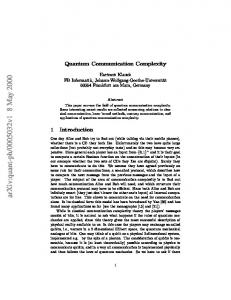
To understand why quantum information can provide a communication advantage without contradicting Holevo’s Theorem, it is necessary to consider more precisely the various scenarios that can be associated with “communication”. The simplest scenario, corresponding to the case covered by Holevo’s Theorem, is illustrated in Fig. 1. There are two parties that we refer to as Alice and Bob. Alice has an n-bit string x Input:
x ∈ {0, 1}n
? '$
Alice
&%
-
communication
Output:
'$
Bob
&% ?
x
Figure 1: The basic communication scenario: Alice receives an n-bit string x as input and sends one message to Bob, who must output x. For this task, a quantum message is no more efficient than a classical message. that she would like to convey to Bob by sending one message. Here it is indeed true, by Holevo’s Theorem [75], that quantum messages are no more efficient than classical messages. Alice must send n qubits to accomplish this specific task. A variant of the communication scenario is where Bob’s goal is not to determine Alice’s data x, but to determine some information that is a function of x in a way that may depend on other 4
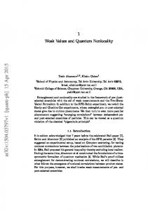
data y that resides with Bob (while y is unknown to Alice). Such a scenario could occur when Alice and Bob each begin with n-bit strings, x and y, respectively (Alice knows x but not y and Bob knows y but not x), and the goal is for Bob to determine the value of some function f (x, y) (where f is known to both parties). An example where such a scenario could arise is where Alice and Bob are interested in scheduling an appointment. Alice’s schedule could be represented by x and Bob’s by y: if there are n time-slots, then we can set the ith bit of x to 1 if Alice is available in time-slot i, and similarly for y. How much communication is required for Bob to find a time when they are both available (i.e., an i such that xi = yi = 1)? We shall see that, for this communication scenario, quantum information enables Alice and Bob to accomplish the task with less (asymptotically less in the number of time-slots) qubit communication than would be required by any protocol that is restricted to classical bit communication. This kind of scenario, illustrated in Fig. 2 (for general functions or relations f on {0, 1}n × {0, 1}n ) is known as communication complexity. It has been extensively studied in the classical Inputs:
y ∈ {0, 1}n
x ∈ {0, 1}n
? '$ �
-
? '$
Bob communication &% &% Alice
?
f (x, y)
Output:
Figure 2: The basic communication complexity scenario: Alice and Bob receive n-bit strings, x and y respectively, as input and their goal to compute some function of these values f (x, y), as Bob’s output. There are tasks of this form where communication in terms of quantum messages is much more efficient than communication in terms of classical messages. The number of qubits can be exponentially smaller than the number of bits. Note that in this framework we do not take into account the time and other resources that Alice and Bob spend locally (although in practice it turns out that their local computations are almost always efficient). case. Indeed, whereas the trivial solution to this problem is for Alice to send Bob her input x, and for Bob to compute f (x, y), it is often possible for Bob to compute f with much less than n bits of classical communication. These savings in classical communication are very interesting both from a practical and a conceptual point of view. Section 3 outlines several of the key results in the area, and we refer the reader to the textbooks [83, 77] for further information. When Alice and Bob can communicate qubits, further reductions in the amount of communication are possible, sometimes even exponential reductions. This remarkable situation is clearly worthy of further study. It is one of the main subjects covered by the present review, and we will see many examples later.
1.3
Quantum non-locality
Long before the work on quantum communication complexity mentioned in the previous section, physicists investigating the foundations of quantum mechanics studied the scenario where local 5
measurements are carried out on two entangled particles. Such entangled states can (at least in principle) be easily produced by having the particles interact together for some time, and then sending the particles away to far-off locations. Local measurements are then carried out on the particles. This scenario was first studied by Einstein, Podolsky, and Rosen [60] and immediately afterwards by Schr¨ odinger [118, 119] (who coined the word entanglement). In these works it was realized that the results of the local measurements would exhibit very interesting correlations. For instance, for some pairs of the measurements, the results may be always the same; for other pairs of measurements, the results may be always opposite, etc. Nevertheless, one can easily show—this follows immediately from the structure of quantum mechanics—that the parties carrying out the measurements cannot use the entangled particles to communicate to each other. More precisely, if two physically separated parties, Alice and Bob, initially possess entangled particles and then Alice is given an arbitrary bit x, there is no way for Alice to manipulate her particles in order to convey any information about x to Bob when he performs measurements on his particles. Given that these correlations cannot be used for communication, one would naively expect that if a (quantum or classical) model can reproduce these correlations, then it is not necessary for that model to use communication. This is indeed the case in the quantum scenario where, having established the entanglement through some interaction in the past, no communication is needed at the time of the measurement. But if one wants to reproduce these correlations in a purely classical model, then classical communication between the parties is required at the moment of the measurements! This situation is even more surprising if the particles are widely separated from each other and the measurements take place during a very short time interval, so short that the two measurement events are space-like separated. In this case the communication would have to occur faster than the speed of light! This remarkable feature of quantum mechanics was discovered by Bell [13], and is now known as “quantum non-locality”. It has been the subject of much further theoretical and experimental study since. Indeed it is one of the most surprising and counter-intuitive features of quantum mechanics. Bell’s Theorem shows that Einstein’s program of trying to rationalize quantum mechanics by reducing it to classical mechanics is futile and doomed to failure, as it cannot be done without giving up another cornerstone of twentieth century physics (discovered by Einstein himself), namely the fact that information cannot travel faster than the speed of light. More recently, another reason why such a reduction is doomed emerged through the study of quantum information. Namely we expect any such classical description of quantum mechanics to be exponentially inefficient, i.e., to use exponentially more resources than the quantum theory. We will discuss quantum non-locality extensively in the present review, focusing on its connection to communication complexity.
1.4
Unity of quantum communication complexity and quantum non-locality
The reason why in this review we deal with quantum communication complexity and quantum non-locality together is that these two topics are intimately related. Indeed they can be formulated in a unified way, and furthermore many questions can be mapped from one topic to the other. In fact, during the past dozen years an intense cross-fertilization has occurred between these two fields, which has considerably enriched both of them. To see the unity between the two subjects, recall that in both cases the parties, Alice and Bob, are given some inputs, x and y. In one case these inputs correspond to the arguments of the function that must be computed. In the other case these inputs correspond to a description of the 6
measurements that must be carried out on the particles (the “measurement settings”). And in both cases Alice and Bob must provide an output, a and b. In communication complexity we require that b = f (x, y) and a is irrelevant; in non-locality we are interested in the correlations between a, b and x, y (for instance we request that a = b when x and y have certain values and that a 6= b when x and y have some other values). We can unify these descriptions by saying that the aim in both cases is to produce a joint probability distribution P (a, b|x, y) of the outputs given the inputs, such that P (a, b|x, y) has certain desirable properties.
1.5
Resources
In both communication and non-locality, the basic question one wants to answer is: what is the minimum amount of resources necessary to reproduce the distribution P (a, b|x, y), and how does this amount change when one changes the model, i.e., when one changes the type of resource that can be used. There are in fact many different types of resources that can be compared, and we now briefly review them. We will come back to them in more detail in the body of the review. • Quantum communication. The parties are allowed to send each other quantum states. One quantifies the amount of communication by the number of qubits sent. • Classical communication. The parties are allowed to send each other classical communication. One quantifies the amount of communication by the number of bits sent. • Entanglement. The parties share entangled states. One quantifies the amount of entanglement by the number of qubits that the state locally consists of. For example we frequently use maximally entangled states of 2 qubits, called ebits (also known as EPR pairs after [60]), √1 (|0i|0i + |1i|1i) or something that can be obtained from this with local operations. 2 • Shared randomness. The parties have randomness, i.e., they are allowed to toss coins. In the case of shared randomness, the parties both share the same string of coins. This could for instance be implemented by having the parties toss the coins beforehand, at some earlier time when they are together, and then use the coins later when they need to solve the communication complexity problem. • Local randomness. The parties have randomness, i.e., they are allowed to toss coins. In the case of local randomness the coins are tossed locally, and the string of outcomes of the coins for Alice is independent of the string of outcomes of the coins for Bob. The rational for measuring classical information in terms of bits is Shannon’s noiseless coding theorem [121], which states that, asymptotically, the information produced by a stochastic source can be encoded in a number of bits equal to the entropy of the source. This is paralleled in the quantum case by Schumacher compression [120], which states that, asymptotically, the information produced by a stochastic quantum source can be encoded into a number of qubits equal to the von Neumann entropy of the source. And it is paralleled in the case of entanglement, by entanglement distillations, namely the fact that pure two-party entangled states can, asymptotically in the number of copies of the state, be converted into the number of ebits equal to the von Neumann entropy 7
of the reduced density matrix of each party [16]. In the context of communication complexity, however, we are not dealing with the asymptotic limit of large amounts of communication or large amounts of entanglement. Thus whereas in most cases we will keep the basic concepts of bits, qubits and ebits, it could be relevant in specific cases to consider variants on these resources, such as trits, non-maximally entangled states, etc. The above resources have been ordered (more or less) from the strongest to the weakest. Indeed most of these resources imply the ones below them. For instance one can send classical information using qubits; one can use quantum communication to distribute entanglement; one can measure the entangled particles to produce shared randomness, etc. The only case where the ordering is not so clear is between classical communication and entanglement. Indeed if two parties share an entangled state, they cannot use it to communicate (as discussed above). But on the other hand (as discussed below) sharing n ebits may allow one to save an exponentially large (in n) amount of bits in some communication scenarios (whereas in all other cases, n uses of one resource allows one to implement n uses of the resources below it). There are also a number of nontrivial ways in which these resources can be substituted one for the other. Quantum teleportation allows one to substitute one ebit and two bits of classical communication for one qubit of quantum communication [14]. Dense coding shows that sharing one ebit and then communicating one qubit allows one to communicate two bits [15]. Newman’s Theorem states that in the context of communication complexity, having shared randomness can save only a small amount of communication compared to having local randomness [101]. In addition we will at some points in this review consider other additional (more specialized or more exotic) resources. For instance one can consider • One-way classical or quantum communication. Alice is allowed to communicate to Bob, but Bob is not allowed to communicate back to Alice. • Simultaneous Message Passing model. In this model there is a third party, called the Referee, and messages are only allowed from Alice to the Referee and from Bob to the Referee. It is the Referee who has to compute the value of the function f (x, y). • Multipartite entanglement. Sometimes one is interested in non-locality or communication complexity between more than two parties. Contrary to bipartite entanglement where it is sufficient to consider ebits, there are many kinds of multiparticle entanglement (such as GHZ states, W states, etc.) which could be useful for solving different communication problems. • Non-local (or PR) boxes. This exotic resource is intermediate between an ebit and a bit. Indeed, it is a resource which does not enable the parties to communicate (in the same way that entanglement does not allow communication). But to be produced physically it requires a bit of communication between the parties at the moment it is used (contrary to entanglement which once established requires no more communication). Its study provides a deeper understanding of the power and limitations of quantum entanglement in communication complexity.
1.6
Basic scenarios
The basic question asked in communication complexity and quantum non-locality is to understand how much of these resources are required in different situations. 8
Thus classical communication complexity [83] is basically concerned with understanding how much classical communication is required to compute the value of a function f (x, y), possibly using (shared or local) randomness. In quantum communication complexity the parties are trying to compute the value of f , but may now use quantum resources. In the quantum communication model, introduced by Yao [137], they can communicate qubits, and in the entanglement model, introduced by Cleve and Buhrman [45], the parties share entangled particles and are allowed to communicate classical bits. When one extends the quantum communication model of Yao such that the parties also share entangled particles, quantum teleportation shows that these two models are essentially equivalent: one qubit in the first model can be replaced by two bits and one ebit in the entanglement, and conversely one bit can be simulated by one qubit. It is, however, a challenging open problem whether the quantum communication model, without shared entanglement, is essentially equivalent to the entanglement model. Non-locality, although at first sight a very different topic, is also concerned with comparing resources. Indeed the basic question in this area is to compare: • The correlations that can be obtained if the parties share entanglement and carry out local measurements on their particles, but are not allowed any communication. • The correlations that can be obtained if the parties have shared randomness, but are not allowed any communication. This is known in the physics literature as a local hidden variable model. Bell’s Theorem states that these two scenarios are not equivalent: shared randomness alone is not sufficient to reproduce the quantum correlations.
1.7
Mappings between communication complexity and non-locality
Thus quantum communication complexity, classical communication complexity, and non-locality can be put in a unified framework in which similar kinds of resources are compared. In addition, in some cases there exist mappings between quantum communication complexity scenarios and non-locality scenarios. The most simple such mapping occurs in the entanglement model if the parties can solve the communication complexity problem more efficiently using entanglement than without entanglement, and if this can be done by measuring their entangled particles before they communicate to each other. Then it immediately follows that the correlations obtained by measuring their entangled particles (but without communicating), cannot be realized in a local hidden variable model. Conversely it is possible to map any non-locality experiment to a communication complexity problem in the entanglement model. This was the approach used in the original paper [45]. It mapped the non-local correlations that arise in the GHZ paradox to a communication complexity problem. This approach has since been generalized [26], although in the resulting communication complexity problem the function f (x, y) is only computed successfully by the parties with non-zero probability. Another mapping can occur in the quantum communication model when one-way quantum communication from Alice to Bob is more efficient than classical communication. Then it is often possible to construct from the communication complexity problem a nontrivial non-locality scenario. This approach has yielded some very interesting non-locality scenarios which we will describe in detail below. 9
1.8
Summary of the review
In this review we will present some of the main results obtained so far in the field of quantum communication complexity. We start by introducing quantum non-locality in Section 2, focusing on its relation with communication complexity. We present simple examples such as the GHZ paradox, the CHSH example, the magic square game, but rephrasing them in the language of data processing. Next we present quantum communication complexity in Section 3, illustrating it with examples such as the distributed Deutsch-Jozsa problem, the intersection problem, Raz’s problem, and the hidden matching problem. In Section 4 we unite these two approaches, showing how some of the examples from quantum communication complexity can be used to derive new non-locality games. In section 5 we discuss another model of communication complexity, the simultaneous message passing model, and show how classical communication, entanglement, quantum communication can be traded one for the other in this model. In Section 6 we discuss several additional aspects of quantum nonlocality, such as non-local boxes, Tsirelson bounds, and simulation of quantum correlations using classical resources. Finally we consider in Section 7 experimental issues, in particular the detection loophole, and present the outlook for future experiments. We conclude by discussing some open questions in the field. The interested reader can also consult the earlier review [20] which covers some of the material presented here.
2
Simple Non-locality Examples
The idea of non-locality was originally concerned with the possibility that quantum mechanics is actually a classical theory that depends on “hidden variables” whose values might be discovered in the future as part of some successor theory to quantum mechanics. Bell [13] proposed a hypothetical experiment for ruling out such classical theories under the assumption that measurements of quantum systems can occur at different points in space-time, and information cannot be transmitted faster than the speed of light. Another way of interpreting Bell’s experiment is as a method for two (or more) cooperating distributed parties to compute some sort of input-output relation, where each party receives input data and must produce output data consistent with the relation. In Bell’s experiment, there is such a task that cannot be accomplished in a setting where the information processing resources are all classical. In contrast, the task can be accomplished if the parties share prior entanglement. Since Bell’s seminal work, the concept of quantum non-locality has been extensively studied, by physicists, philosophers, and more recently by computer scientists. Some of the important early advances have been the Clauser-Horn-Shimony-Holt (CHSH) inequality [44] which allows Bell’s surprising predictions to be tested even in the presence of noise; and the GHZ-Mermin scenario [72, 94] which was the first ”pseudo-telepathy” game. More recently there has been a more or less systematic enumeration of Bell inequalities for small number of settings and/or outcomes (see, e.g., [49, 48, 134, 141]); the study of the statistical power of non-locality tests [52]; an understanding of the limits to quantum non-locality (Tsirelson-type bounds) [43] as compared to the larger world of correlations obeying only the no-signalling conditions (e.g., non-local boxes); investigations of the power of non-locality in cryptographic settings [11], etc. In the next paragraphs we review various non-locality scenarios, casting them in the language of data processing. The reader wishing to complement this overview could consult two recent reviews, written more from physics [135] and computer science [21] perspectives.
10
2.1
GHZ: Greenberger-Horne-Zeilinger and Mermin
The following scenario essentially underlies those of [72, 94], but is cast in the language of data processing. The basic structure is illustrated in Fig. 3. Three physically separated parties—call Inputs:
s ? '$
Alice
&% ?
Outputs:
a
t ? '$
Bob
&% ?
b
u ? '$
Carol
&% ?
c
Figure 3: The general form of a non-locality scenario involving three parties: Alice, Bob, and Carol receive inputs s, t, u respectively, and are required to produce outputs a, b, c, respectively, satisfying certain conditions. Once the inputs are received, no communication is permitted between the parties. For the specific GHZ scenario, it is possible to accomplish the task if the parties are in possession of a tripartite entangled state. Without the prior entanglement, it is impossible to accomplish the task. them Alice, Bob, and Carol—receive input bits s, t, and u, respectively, which are arbitrary subject to the condition that s ⊕ t ⊕ u = 0 (⊕ denotes exclusive or, which is the sum of its arguments in modulo 2 arithmetic). Once they receive their input data, they are forbidden from having any communication between them. Their goal is to produce output bits a, b, and c, respectively, such that ( 0 if stu = 000 (1) a⊕b⊕c= 1 if stu ∈ {011, 101, 110}. Note that the task that the three parties are trying to accomplish is the computation of a relation, where there are three input bits (stu) and three output bits (abc). The task is nontrivial in light of the fact that the input bits are distributed among the parties so that each party is given the value of only one of them; the output bits are also distributed. The first observation is that with classical resources there must be communication among the three parties to succeed. To see why this is so, first consider deterministic strategies (later we will analyze the case of probabilistic strategies, where the parties behave stochastically, i.e., they can flip coins). Since Alice cannot receive any information from Bob or Carol, her output bit a can depend only on the value of her input bit s. Let a0 (respectively a1 ) be Alice’s output when her input bit is 0 (respectively 1). Similarly, let b0 , b1 and c0 , c1 be Bob and Carol’s outputs for their respective input values. Note that the six bits a0 , a1 , b0 , b1 , c0 , c1 completely characterize any deterministic strategy of Alice, Bob, and Carol. The conditions of the problem translate into the
11
equations a0 ⊕ b0 ⊕ c0 = 0,
a0 ⊕ b1 ⊕ c1 = 1,
a1 ⊕ b0 ⊕ c1 = 1,
a1 ⊕ b1 ⊕ c0 = 1.
(2)
It is impossible to satisfy all four equations simultaneously. This is because summing the four equations modulo two, yields 0 = 1 (recall that 1 + 1 = 0 modulo 2). Therefore, for any strategy, there exists an input configuration stu ∈ {000, 011, 101, 110} for which it fails. Note however that for any three out of the four equations from (2) there is a strategy that satisfies these three equations perfectly. To see why probabilistic strategies cannot succeed either, note that any such strategy can be modeled as a deterministic strategy where Alice, Bob, and Carol have access to a random variable r (for example, r could be the outcomes of a sequence of uniformly distributed random bits). This r is sometimes referred to as a “local hidden variable”. It is assumed that the testing procedure does not have access to r, so that the input bits (stu) are uncorrelated with r. The intuitive way of thinking about this scenario is that the three parties get together before the game starts, randomly select r, and then each party secretly keeps a copy of this information. An example of a probabilistic strategy is for r ∈ {0, 1}2 to be two uniformly random bits that specify which three of the four equations in (2) are satisfied. This probabilistic strategy succeeds with probability 3/4. We next show that this success probability is optimal. Suppose that the input data s, t, u is uniformly distributed over {000, 011, 101, 110}. Then the success probability that any randomized protocol achieves is X r
qr
1X P (s, t, u, r), 4 s,t,u
(3)
where qr is the probability (of the shared randomness) that the parties flip r, and P (s, t, u, r) = 1 if the deterministic protocol corresponding to r is correct on input stu and P (s, t, u, r) = 0 otherwise. Clearly this is bounded above by 1X P (s, t, u, r), (4) max r 4 s,t,u which by the above discussion is at most 3/4. Now consider the same problem, but where Alice, Bob, and Carol have an additional resource: each is supplied with a qubit, where the state of the combined 3-qubit system is1 1 2 |000i
− 21 |011i − 21 |101i − 12 |110i.
(5)
The parties are allowed to apply unitary transformations and perform measurements on their individual qubits, but communication between the parties is still forbidden. It turns out that now the parties can produce a, b, c satisfying Eq. (1). This is achieved by the procedure that follows. The procedure for Alice is to measure her qubit in the computational basis (consisting of |0i and |1i) if her input bit s is 0, and to measure her qubit in the Hadamard basis (consisting of 1
This is an entangled state that is equivalent to the so-called GHZ state operations).
12
1 √ |000i 2
+
√1 |111i 2
(under local unitary
H|0i = √12 (|0i + |1i) and H|1i = √12 (|0i − |1i)) if her input bit is 1. In either case, she sets her output bit a to the outcome of her measurement. The procedures for Bob and Carol are similar to that of Alice, but with Bob’s bits being s and b, and Carol’s bits being u and c. To see why the described procedure always produces output bits abc satisfying Eq. (1), consider the various cases of the input possibilities stu. In the case where stu = 000, the state is measured in the computational basis, so clearly the outcomes are from {000, 011, 101, 110}, and hence satisfy a ⊕ b ⊕ c = 0. The case where stu = 011 can be analyzed by assuming that a Hadamard transform is applied to the last two qubits of the state prior to a measurement in the computational basis. Since (I ⊗ H ⊗ H) ( 12 |000i − 21 |011i − 21 |101i − 12 |110i) 1 1 2 |0i(|00i − |11i) − 2 |1i(|01i + |10i) − 21 |1i(|00i − |11i) 1 1 1 2 |010i − 2 |100i + 2 |111i,
= (I ⊗ H ⊗ H) =
=
1 2 |0i(|01i 1 2 |001i +
� + |10i) (6)
a ⊕ b ⊕ c = 1, as required, in this case. The remaining cases where stu = 101 and 110 are similar by the symmetry of the entangled state and protocol. We have shown that the entangled state enables the three parties to correlate their output bits with their inputs bits in a manner that is impossible to achieve with classical resources, unless there is communication among the parties. It should be noted that, in accomplishing this task using the entangled state, no actual communication occurs among the parties. In particular, the output bits a, b, and c individually contain no information about stu; they are uniformly distributed in all cases. It is only the trivariate correlations among a, b, and c that are related to the input data stu.
2.2
CHSH: Clauser-Horne-Shimony-Holt
The following scenario essentially underlies that of [44] but is cast in the language of data processing. The basic structure is illustrated in Fig. 4. Alice and Bob receive input bits s and t, respectively, Inputs:
t
s ? '$
Alice
&% ?
Outputs:
? '$
Bob
&% ?
b
a
Figure 4: The non-locality scenario involving two parties: Alice and Bob receive inputs s and t respectively, and are required to produce outputs a and b respectively, satisfying certain conditions. Once the inputs are received, no communication is permitted between the parties. For the specific CHSH scenario, it is possible to accomplish the task with probability cos2 (π/8) = 0.853 . . . if the parties are in possession of an ebit. Without the prior entanglement, the highest possible success probability is 3/4.
13
and, after this, they are forbidden from communicating with each other. Their goal is to produce output bits a and b, respectively, such that a ⊕ b = s ∧ t,
(7)
(‘∧’ is the logical and, which is 1 if all its arguments are 1, and which is 0 otherwise) or, failing that, to satisfy this condition with as high a probability as possible. To analyze the situation in terms of classical information, first again consider the case of deterministic strategies. For these, Alice’s output bit depends solely on her input bit s and similarly for Bob. Let a0 , a1 be the two possibilities for Alice and b0 , b1 be the two possibilities for Bob. These four bits completely characterize any deterministic strategy. Condition (7) translates into the equations a0 ⊕ b0 = 0,
a0 ⊕ b1 = 0,
a1 ⊕ b0 = 0,
a1 ⊕ b1 = 1.
(8)
It is impossible to satisfy all four equations simultaneously (since summing them modulo 2 yields 0 = 1). Therefore it is impossible to satisfy Condition (7) absolutely. By using a probabilistic strategy, Alice and Bob can satisfy Condition (7) with probability 3/4. For such a strategy, we allow Alice and Bob to have a priori classical random variables, whose distribution is independent of that of the inputs s and t. Note that any three of the four equations of (8) can be simultaneously satisfied. The probabilistic classical strategy works as follows. Alice and Bob have uniformlydistributed random bits that are used to specify which of the four equations of (8) is violated, and then play the strategy that satisfies the other three perfectly. It is easy to see that (a) for any input st, the resulting outputs satisfy Condition (7) with probability 3/4, and (b) this is optimal in that no probabilistic strategy can attain a success probability greater than 3/4. Now consider the same problem but where Alice and Bob are each supplied with a qubit where the state of the two-qubit system is initialized to √1 (|00i 2
− |11i).
(9)
It turns out that now the parties can produce data that satisfies Condition (7) with probability cos2 (π/8) = 0.853 . . ., which is higher than what is possible in the classical case. This is achieved by the following procedures. Denote the unitary operation that rotates the qubit by angle θ by � � cos θ − sin θ R(θ) = (where we have written it out in the computational basis). Alice applies sin θ cos θ one of two rotations on her qubit, depending on her input bit s: if s = 0 the rotation is R(−π/16); if s = 1 the rotation is R(3π/16). Then Alice measures her qubit in the computational basis and sets her output bit a to the result. Bob’s procedure is the same, depending on his input bit t. It is straightforward to calculate that, if Alice rotates by θ1 and Bob rotates by θ2 , then the entangled state becomes √1 (cos(θ1 + θ2 )(|00i − |11i) + sin(θ1 + θ2 )(|01i + |10i)). (10) 2 After the measurements, the probability that a ⊕ b = 0 is cos2 (θ1 + θ2 ). It is now a straightforward exercise to verify that Condition 7 is satisfied with probability cos2 (π/8) for all four input possibilities. 14
2.3
Tsirelson’s upper bound for CHSH
Although the protocol in the previous subsection using entanglement has a higher success probability (cos2 (π/8) = 0.853 . . .) than any classical protocol (3/4), it still does not succeed with probability 1. This raises the question of whether there is a different strategy using entanglement that always succeeds—or, failing that, whose success probability exceeds cos2 (π/8). Tsirelson [43] first showed that the above quantum protocol is optimal in that it is impossible to exceed success probability cos2 (π/8), regardless of the strategy—including any amount of prior entanglement—the parties start with. What follows is a simple proof of this result. Consider an arbitrary bipartite entangled state |ψiAB . An arbitrary strategy for Alice that uses this entangled state can be represented by two observables2 A0 and A1 , each with eigenvalues in {+1, −1}. When Alice’s input bit is 0, she obtains her output bit by applying the projective measurement corresponding to the eigenspaces of A0 to the component of |ψiAB in her possession. The +1-eigenspace of A0 corresponds to output bit 0, while the −1-eigenspace corresponds to the output bit 1. When her input bit is 1, she applies the measurement corresponding to A1 . Similarly, an arbitrary strategy for Bob can be represented by two observables B0 and B1 . At this point, the reader might object that |ψiAB , A0 , A1 , B0 , and B1 do not capture every possible strategy of Alice and Bob, since they need not be limited to applying projective measurements. Although non-projective measurements may be used, such measurements can always be simulated by projective measurements in a larger Hilbert space. Thus, no generality has been lost because any strategy can be converted to the above form. Since the observables have eigenvalues in {+1, −1} rather than {0, 1}, it is more convenient here to think of Alice and Bob’s output bits in these terms as a′ = (−1)a and b′ = (−1)b , respectively. Then the protocol succeeds on input st if and only if (−1)s∧t · a′ · b′ = 1. If s and t are randomly chosen according the uniform distribution, then the expected value of (−1)s∧t · a′ · b′ is � (11) hψ|AB 14 A0 ⊗ B0 + 41 A0 ⊗ B1 + 41 A1 ⊗ B0 − 14 A1 ⊗ B1 |ψiAB , and is therefore upper bounded by the largest eigenvalue of
M = 14 A0 ⊗ B0 + 41 A0 ⊗ B1 + 41 A1 ⊗ B0 − 14 A1 ⊗ B1 .
(12)
It is straightforward to calculate that 1 1 1 1 M 2 = 41 I − 16 (A0 A1 )⊗(B0 B1 )+ 16 (A0 A1 )⊗(B1 B0 )+ 16 (A1 A0 )⊗(B0 B1 )− 16 (A1 A0 )⊗(B1 B0 ), (13)
from which we can upper bound the maximum eigenvalue of M 2 by the sum of the maximum 1 1 1 1 + 16 + 16 + 16 = 12 . It follows that the largest eigenvalue eigenvalue in each term, obtaining 14 + 16 √ of M itself is at most 1/ 2, which therefore upper bounds the expected value of (−1)s∧t · a′ · b′ . √ This translates into an upper bound of (1 + 1/ 2)/2 = cos2 (π/8) for the success probability of the actual protocol (where Alice and Bob output bits a and b). This completes the proof of Tsirelson’s upper bound for CHSH. 2
An observable is a Hermitian operator. One associates to an observable a projective measurement, with one projector for each of the eigenspaces of the observable.
15
2.4
Magic square game
In one respect the GHZ example is more striking than the CHSH example: in the former case, the protocol with entanglement always succeeds, while in the latter case the protocol with entanglement merely succeeds with higher probability. However, the GHZ example involves three parties, whereas the CHSH example only involves two. Is there a two-party scenario where the quantum protocol always succeeds, whereas the best classical success probability is bounded below 1? The answer is affirmative, see for instance [38, 37, 39]. A particularly elegant example is the following game, which has been referred to as the magic square game [5]. To define this game, consider the problem of labeling the entries of a 3 × 3 matrix with bits so that the parity of each row is even, whereas the parity of each column is odd. It is not hard to see that this is impossible3 . The two matrices 0 0 1
0 0 1
0 0 0
0 0 1
0 0 1
0 0 1
each satisfy five out of the six constraints. For the first matrix, all rows have even parity, but only the first two columns have odd parity. For the second matrix, the first two rows have even parity, and all columns have odd parity. Bearing the above in mind, consider the game where Alice receives s ∈ {1, 2, 3} as input (specifying the number of a row), and Bob receives t ∈ {1, 2, 3} as input (specifying the number of a column). Their goal is to each produce 3-bit outputs, a1 a2 a3 for Alice and b1 b2 b3 for Bob, with these properties: 1. They satisfy the row/column parity constraints. Namely, a1 ⊕ a2 ⊕ a3 = 0 and b1 ⊕ b2 ⊕ b3 = 1. 2. They are consistent where the row intersects the column. Namely, at = bs . As usual, Alice and Bob are forbidden from communicating once the game starts, so Alice does not know what t is and Bob does not know what s is. We shall observe that, classically, the best success probability possible is 8/9, whereas there is a quantum strategy that always succeeds. An example of a strategy that attains success probability 8/9 (when the input st is uniformly distributed) is where Alice plays according to the rows of the first matrix above and Bob plays according the columns of the second matrix above. This succeeds in all cases, except where s = t = 3. To see why this is optimal, note that for any other classical strategy, it is possible to represent it as two matrices as above but with different entries. Alice plays according to the rows of the first matrix and Bob plays according to the columns of the second matrix. We can assume that the rows of Alice’s matrix all have even parity; if she outputs a row with odd parity then they immediately lose, regardless of Bob’s output. Similarly, we can assume that all columns of Bob’s matrix have odd parity.4 Considering such a pair matrices, the players lose at each entry where they differ. There must be such an entry, since otherwise it would be possible to have all rows even and all columns odd with one matrix. Thus, when the input st is chosen uniformly from {1, 2, 3}× {1, 2, 3}, the success probability is at most 8/9. 3
As before, we can express a valid solution in terms of equations, in this case six of them (where arithmetic is modulo 2): m11 +m12 +m13 = 0, m21 +m22 +m23 = 0, m31 +m32 +m33 = 0, m11 +m21 +m31 = 1, m12 +m22 +m32 = 1, m13 + m23 + m33 = 1. Adding these equations modulo 2 yields 0 = 1. 4 In fact, the game can be simplified so that Alice and Bob each output just two bits, since the parity constraint determines the third bit.
16
The quantum strategy for this game is based on the following observation due to Mermin [93, 95]. Let I, X, Y , Z denote the 2 × 2 Pauli matrices: � � � � � � � � 1 0 0 −i 0 1 1 0 . (14) , and Z = , Y = , X= I= 0 −1 i 0 1 0 0 1 Each is an observable with eigenvalues in {+1, −1}. Consider the following table of two-qubit observables that are each a tensor product of two Pauli matrices: X ⊗X Y ⊗Y Z⊗Z
Y ⊗Z Z⊗X X ⊗Y
Z⊗Y X ⊗Z Y ⊗X
For our present purposes, the noteworthy property is that the observables along each row commute and their product is I ⊗ I, and the observables along each column commute and their product is −I ⊗ I. This implies that, for any two-qubit state, performing the three measurements along any row results in three {+1, −1}-valued bits whose product is +1. Also, performing the three measurements along any column results in three {+1, −1}-valued bits whose product is −1. This can be seen more easily when one simultaneously diagonalizes the three commuting observables. They will have 1 and −1 eigenvalues on the diagonal. Each consecutive observable will project the state onto a possible refinement of the current eigenspace the state lies in. This will yield that the product of the outcomes of the three observables will be 1 in case the observables belong to a row of the matrix, because the product of the row observables is I ⊗ I, and −1 when they belong to a column, since the product of the observables for each column is −I ⊗ I. We can now describe the quantum protocol. It uses two pairs of entangled qubits, each of which is in initial state √12 (|01i − |10i). Alice, on input s, applies three two-qubit measurements corresponding to the observables in row s of the above table. For each measurement, if the result is +1, she outputs 0 and if the result is −1, she outputs 1. Similarly, Bob, on input t, applies the measurements corresponding to the observables in column t, and converts the outcomes into bits in the same manner. We have already established that Alice and Bob’s output bits satisfy the required parity constraints. It remains to show that Alice and Bob’s output bits that correspond to where the row meets the column are the same. For that measurement, Alice and Bob are measuring with respect to the same observable in the above table. Because all the observables in each row and in each column commute, we may assume that the place where they intersect is the first observable applied. Those bits are obtained by Alice and Bob each measuring 12 (|01i − |10i)(|01i − |10i) with respect to the observable in entry (s, t) of the table. To show that their measurements will agree for all cases of st, we consider the individual Pauli measurements on the individual entangled pairs of the form √1 (|01i − |10i). Let a′ and b′ denote the outcomes of the first measurement (in terms of bits), and 2 a′′ and b′′ denote the outcomes of the second. Since the measurement associated with the tensor product of two observables is operationally equivalent to measuring each individual observable and taking the product of the results, we have that at = a′ ⊕ a′′ and bs = b′ ⊕ b′′ . It is straightforward to verify that if the same measurement from {X, Y, Z} is applied to each qubit of √12 (|01i − |10i) then the outcomes will be distinct. Therefore, a′ ⊕ b′ = 1 and a′′ ⊕ b′′ = 1, from which it follows
17
that at ⊕ bs = (a′ ⊕ a′′ ) ⊕ (b′ ⊕ b′′ )
= (a′ ⊕ b′ ) ⊕ (a′′ ⊕ b′′ ) = 1⊕1 = 0,
(15)
so at = bs . This completes the analysis of the magic square game.
3
Communication Complexity
In the last section we considered scenarios without communication. Here we will extend the nonlocality setting to one where the parties (Alice and Bob) are allowed to send information to each other in the form of bits or qubits. They can still have shared randomness and may share an entangled quantum state. We are now interested in the minimum number of bits or qubits that are needed in order to compute a function that depends on the inputs of all the parties. The ability to send information to each other departs from the setting of non-locality. We will see that entanglement can be used to reduce (for certain functions) the communication drastically compared to when the parties share just classical resources. Accordingly, while entanglement cannot be used for signalling, it can be used to significantly reduce the communication needed for certain tasks. In later sections we will see how some of the ideas and protocols developed in the setting of communication complexity can be used to formulate new non-locality games. Communication complexity has been studied extensively in the area of theoretical computer science and has deep connections with seemingly unrelated areas, such as VLSI design, circuit lower bounds, lower bounds on branching programs, size of data structures, and bounds on the length of logical proof systems, to name just a few. We refer to the textbooks [83, 77] for more details.
3.1
The setting
First we sketch the setting for classical communication complexity. Alice and Bob want to compute some function f : D → {0, 1}, where D ⊆ X × Y . If the domain D equals X × Y then f is called a total function, otherwise it is a promise function. Alice receives input x ∈ X, Bob receives input y ∈ Y , with (x, y) ∈ D. A typical situation, illustrated in Fig. 2, is where X = Y = {0, 1}n , so both Alice and Bob receive an n-bit input string. As the value f (x, y) will generally depend on both x and y, some communication between Alice and Bob is required in order for them to be able to compute f (x, y). We are interested in the minimal amount of communication they need. A communication protocol is a distributed algorithm where first Alice does some individual computation, and then sends a message (of one or more bits) to Bob, then Bob does some computation and sends a message to Alice, etc. Each message is called a round. After one or more rounds the protocol terminates and outputs some value, which must be known to both players. The cost of a protocol is the total number of bits communicated on the worst-case input. A deterministic protocol for f always has to output the right value f (x, y) for all (x, y) ∈ D. In a bounded-error protocol, Alice and Bob may flip coins and the protocol has to output the right value f (x, y) with probability ≥ 2/3 for all (x, y) ∈ D. We could either allow Alice and Bob to toss coins individually 18
(local randomness, or “private coin”) or jointly (shared randomness, or “public coin”). The later is analogous to the local hidden variables in non-locality games. A public coin can simulate a private coin and is potentially more powerful. However, Newman’s theorem [101] says that having a public coin can save at most O(log n) bits of communication, compared to a protocol with a private coin. Some often studied functions are: • Equality: EQ(x, y) = 1 if x = y, and EQ(x, y) = 0 otherwise P • Inner product: IP(x, y) = ni=1 xi yi (mod 2) (for x, y ∈ {0, 1}n , xi is the ith bit of x)
• Intersection: INT(x, y) = 1 if there is an i where xi = yi = 1, and INT(x, y) = 0 otherwise (viewing x as corresponding to the set {i : xi = 1} and similarly for y, INT(x, y) says whether the sets x and y intersect). A variant of this problem asks to actually find an i where xi = yi = 1, or to output that none such i exists.
Let us first consider the equality problem, which will recur throughout the text. The goal for Alice is to determine whether her n-bit input is the same as Bob’s or not. It is not hard to show that in the deterministic case, n bits of communication are needed (see Section B.1 of the appendix for a proof), so Bob might as well send his string to Alice after which Alice announces the answer to Bob with one more bit. To illustrate the power of randomness, let us give a simple yet efficient bounded-error protocol for the equality problem. Alice and Bob jointly toss a random string r ∈ {0, 1}n . Alice sends the bit a = x · r to Bob (where ‘·’ is inner product mod 2). Bob computes b = y · r and compares this with a. If x = y then a = b, but if x 6= y then a 6= b with probability 1/2. Repeating this a few times, Alice and Bob can decide equality with small error using O(n) public coin flips and a constant amount of communication. This protocol uses public coins, but note that Newman’s theorem implies that there exists an O(log n)-bit protocol that uses a private coin. Let us explicitly describe such a protocol. Alice views herPn bits as the coefficients of a polynomial px over some finite field F of about 3n elements:5 px (t) = ni=1 xi ti−1 . She picks a random element a ∈ F, and sends Bob the pair a, px (a), which she can do using 2 log(3n) bits. Bob computes py (a) and outputs 1 if px (a) = py (a), and outputs 0 otherwise. Clearly, if x = y then Bob always outputs the correct answer 1. However, if x 6= y then the polynomial px (t) − py (t) is a polynomial in t of degree at most n − 1 that is not identically equal to 0. Such a polynomial can be 0 on at most n − 1 elements of F. Hence with probability at least 2/3, the field element a that Alice chose satisfies px (a) 6= py (a), and Bob will give the correct output 0 also in this case.
3.2
The quantum question
Now what happens if we give Alice and Bob a quantum computer and allow them to send each other qubits and/or to make use of ebits that they share at the start of the protocol? Formally speaking, we can model a quantum protocol as follows. The total state consists of 3 parts: Alice’s private space, the channel, and Bob’s private space. The starting state is |xi|0i|yi: Alice gets x, the channel is initialized to 0, and Bob gets y. Now Alice applies a unitary transformation to her space and the channel. This corresponds to her private computation as well 5 For those not familiar with finite fields: it suffices to choose a prime number p ≈ 3n and do all additions and multiplications modulo this p.
19
as to putting a message on the channel (the length of this message is the number of channel-qubits affected by Alice’s operation). Then Bob applies a unitary transformation to his space and the channel, etc. At the end of the protocol Alice or Bob makes a measurement to determine the output of the protocol. This model was introduced by Yao [137]. In the second model, introduced by Cleve and Buhrman [45], Alice and Bob share an unlimited number of ebits at the start of the protocol, but now they communicate via a classical channel: the channel has to be in a classical state throughout the protocol. We only count the communication, not the number of ebits used. Protocols of this kind can simulate protocols of the first kind with only a factor 2 overhead: using teleportation, the parties can send each other a qubit using an ebit and two classical bits of communication. Hence the qubit-protocols that we describe below also immediately yield protocols that work with entanglement and a classical channel. Note that an ebit can simulate a public coin toss: if Alice and Bob each measure their half of the pair of qubits, they get the same random bit. The third variant combines the strengths of the other two: here Alice and Bob start out with an unlimited number of ebits and they are allowed to communicate qubits. This third kind of communication complexity is in fact equivalent to the second, up to a factor of 2, again by teleportation. Before continuing to study this model, we first have to face an important question, already mentioned in the introduction: is there anything to be gained here? At first sight, the following argument seems to rule out any significant gain. Suppose that in the classical world k bits have to be communicated in order to compute f . Since Holevo’s theorem says that k qubits cannot contain more information than k classical bits, it seems that the quantum communication complexity should be roughly k qubits as well (maybe k/2 to account for superdense coding, but not less). Surprisingly (and fortunately for us), this argument is false, and quantum communication can sometimes be much less than classical communication complexity. The information-theoretic argument via Holevo’s theorem fails, because Alice and Bob do not need to communicate the information in the k bits of the classical protocol; they are only interested in the value f (x, y), which is just 1 bit. Below we will survey some of the main examples that have so far been found of differences between quantum and classical communication complexity.
3.3
The first examples
Quantum communication complexity was introduced by Yao [137] and studied by Kremer [82], but neither showed any advantages of quantum over classical communication. Cleve and Buhrman [45] introduced the variant with classical communication and prior entanglement, and exhibited the first quantum protocol provably better than any classical protocol. It uses quantum entanglement to save 1 bit of classical communication. This gap was extended by Buhrman, Cleve, and van Dam [31] and, for arbitrary k parties, by Buhrman, van Dam, Høyer, and Tapp [34].
3.4
Distributed Deutsch-Jozsa
The first impressively large gaps between quantum and classical communication complexity were exhibited by Buhrman, Cleve, and Wigderson [33]. Their protocols are distributed versions of known quantum query algorithms, like the Deutsch-Jozsa [56] and Grover [74] algorithms. Let us start with the first one. It is actually explained most easily in a direct way, without reference to the Deutsch-Jozsa algorithm (though that is where the idea came from). The problem
20
deals with a promise version of the equality problem. Suppose the n-bit inputs x and y are restricted to the following case: DJ promise: either x = y, or x and y differ in exactly n/2 positions Note that this promise only makes sense if n is an even number, otherwise n/2 would not be integer. In fact it will be convenient to assume n a power of 2. Here is a simple quantum protocol to solve this promise version of equality using only log n qubits: P 1. Alice sends Bob the log n-qubit state √1n ni=1 (−1)xi |ii, which she can prepare unitarily from x and log n |0i-qubits. 2. Bob applies the unitary map |ii 7→ (−1)yi |ii to the state, applies a Hadamard transform to each qubit (for this it is convenient to view i as a log n-bit string), and measures the resulting log n-qubit state. 3. Bob outputs 1 if the measurement gave |0log n i and outputs 0 otherwise. It is clear that this protocol only communicates log n qubits, but why does it work? Note that the state that Bob measures is ! n n X X 1X 1 (−1)i·j |ji (−1)xi +yi (−1)xi +yi |ii = H ⊗ log n √ n n log n i=1
i=1
j∈{0,1}
ThisP superposition looks rather unwieldy, but consider the amplitude of the |0log n i basis state. It 1 is n ni=1 (−1)xi +yi , which is 1 if x = y and 0 otherwise because the promise now guarantees that x and y differ in exactly n/2 of the bits! Hence Bob will always give the correct answer. What about efficient classical protocols (without entanglement) for this problem? Proving lower bounds on communication complexity often requires a very technical combinatorial analysis. Buhrman, Cleve, and Wigderson used a deep combinatorial result of Frankl and R¨ odl [62] to prove that every classical errorless protocol for this problem needs to send at least 0.007n bits. We give the details in Appendix B.4. This log n-qubits-vs-0.007n-bits example was the first exponentially large separation of quantum and classical communication complexity. Notice, however, that the difference disappears if we move to the bounded-error setting, allowing the protocol to have some small error probability. We can use the randomized protocol for equality discussed above or even simpler: Alice can just send a few (i, xi ) pairs to Bob, who then compares the xi ’s with his yi ’s. If x = y he will not see a difference, but if x and y differ in n/2 positions, then Bob will probably detect this. Hence O(log n) classical bits of communication suffice in the bounded-error setting, in sharp contrast to the errorless setting.
3.5
The Intersection problem
Now consider the Intersection function, which is 1 if xi = yi = 1 for at least one i. Note that this is a decision problem of the appointment-scheduling problem mentioned in the introduction. Buhrman, Cleve, and Wigderson [33] also presented an efficient quantum protocol for this. Their protocol is based on Lov Grover’s famous quantum search algorithm [74], which we will briefly sketch here.
21
Suppose there is some n-bit string z and we would like to find an index i such that zi = 1. We cannot “look” at z directly, but we can apply the following unitary map: Oz : |ii 7→ (−1)zi |ii. Grover’s algorithm starts in a uniform superposition following unitary Grover iterate to the state:
√1 n
Pn
i=1 |ii
and then repeatedly applies the
G = H ⊗ log n O0 H ⊗ log n Oz , where H ⊗ log n is the log n-qubit Hadamard transform, and O0 is the unitary that puts a ‘−’ in front of the all-0 state. Suppose there are exactly t solutions: t indices i where zi = 1. p We will not π give the analysis here (see for instance [24]), but one can show that after about 4 n/t Groveriterations, most of the amplitude of the state sits on such solutions. Measuring the state will now with high probability give us a solution. Of course we may not know t in advance, but there is a √ way to find a solution with high probability using O( n) Grover-iterates even in that case. Now what about the Intersection problem? Note that we just want to find a solution for the string z = x ∧ y, which is the bit-wise AND of x and y, since zi = 1 whenever both xi = 1 and yi = 1. The idea is now to let Alice run Grover’s algorithm to search for such a solution. Clearly, she can prepare the uniform starting state herself. She can also apply H and O0 herself. The only thing where she needs Bob’s help, is in implementing Oz . This they do as follows. Whenever Alice want to apply Oz to a state n X αi |ii, |φi = i=1
she tags on her xi in an extra qubit and sends Bob the state n X i=1
αi |ii|xi i.
Bob applies the unitary map |ii|xi i 7→ (−1)xi ∧yi |ii|xi i and sends back the result. Alice sets the last qubit back to |0i (which she can do unitarily because she has x), and now she has the state Oz |φi! Thus we can simulate Oz using 2 messages of log(n)+1 √ qubits each. Thus Alice and Bob can run Grover’s algorithm to find an intersection, using O( n) √ messages of O(log n) qubits each, for total communication of O( n log n) qubits. Later Aaronson √ and Ambainis [1] gave a more complicated protocol that uses O( n) qubits of communication. What about lower bounds? It is a well-known result of classical communication complexity that classical bounded-error protocols for the Intersection problem need about n bits of communication [78, 111]. Thus we have a quadratic quantum-classical separation for this problem. Could the separation be even bigger than quadratic? This question was open for quite a few years after [33] appeared, until finally Razborov [112] showed that any bounded-error quantum protocol for Inter√ section needs to communicate about n qubits. His proof is beautiful but deep and complicated. We sketch it in Appendix C.
22
3.6
Raz’s problem
Notice the contrast between the examples of the last two sections. For the Distributed DeutschJozsa problem we get an exponential quantum-classical separation, but the separation only holds if we require the classical protocol to be errorless. On the other hand, the gap for the disjointness function is only quadratic, but it holds even if we allow classical protocols to have some error probability. Raz [110] exhibited a function where the quantum-classical separation has both features: the quantum protocol is exponentially better than the classical protocol, even if the latter is allowed some error probability. Consider the following promise problem P: Alice receives a unit vector v ∈ Rm and a decomposition of the corresponding space in two orthogonal subspaces H (0) and H (1) . Bob receives an m × m unitary transformation U . Promise: U v is either “close” to H (0) or to H (1) (more precisely, letting P be the projector on subspace H, a vector v is close to H if kP vk2 ≥ 2/3). Question: which of the two? As stated, this is a problem with continuous input, but it can be discretized in a natural way by approximating each real number by O(log m) bits. Alice and Bob’s input is now n = O(m2 log m) bits long. There is a simple yet efficient 2-round quantum protocol for this problem: Alice views v as a log m-qubit vector and sends this to Bob. Bob applies U and sends back the result. Alice then measures in which subspace H (i) the vector U v lies and outputs the resulting i. This takes only 2 log m = O(log n) qubits of communication. The efficiency of this protocol comes from the fact that an m-dimensional unit vector can be “compressed” or “represented” as a log m-qubit state. Similar compression is not possible with classical bits, which suggests that any classical protocol for P will have to send the vector v more or less literally and hence will require a lot of communication. This turns out to be true but the proof (given in [110]) is surprisingly hard. It shows that any bounded-error protocol for P needs to send at least about n1/4 / log n bits.
3.7
The Hidden Matching problem
Consider the following promise problem HM from [9], for even integer n: Alice receives a string x ∈ {0, 1}n . Bob receives a perfect matching M on {1, . . . , n} (i.e., a partition into n/2 disjoint pairs M = {(i1 , j1 ), . . . , (in/2 , jn/2 )}). Question: output a triple (i, j, xi ⊕ xj ) for some (i, j) ∈ M . This communication problem is not a function, but a relation: for each input-pair x, M there are n/2 different correct answers instead of only one: (i, j, xi ⊕ yi ) is correct for each (i, j) ∈ M . We consider one-way protocols here, where Alice sends one message to Bob and then Bob should produce a triple (i, j, xi ⊕ xj ). We now describe a quantum protocol where Alice sends only O(log n) qubits and Bob gives one of the correct answers with probability 1 [9]. Alice sends Bob the following log n-qubit message: n
1 X √ (−1)xi |ii. n i=1
23
Bob views M as an orthogonal decomposition of the space Cn into n/2 2-dimensional subspaces. For instance, the projector for the subspace corresponding to (i, j) ∈ M would be Pij = |iihi| + |jihj|. Bob applies this measurement on the state he received, and obtains the label of some random (i, j) ∈ M as well as the projected state 1 √ ((−1)xi |ii + (−1)xj |ji) . 2 An appropriate measurement on this state will give Bob the bit xi ⊕ xj with certainty, and he can output the correct answer (i, j, xi ⊕ xj ). What about classical protocols? First note that the HM problem can be solved by a short classical message from Bob to Alice: Bob sends Alice a pair (i, j) ∈ M using 2 log n bits, which allows Alice to compute xi ⊕ xj . But the situation is radically different if we consider classical one-way communication from Alice to Bob only. Indeed, one can show that if Alice sends Bob pairs √ (i, xi ) for O( n) randomly chosen i’s, then Bob probably received both points from at least one pair in M 6 . This allows him to output a correct answer. On the other hand, Bar-Yossef, Jayram, and Kerenidis [9] proved that any classical protocol solving the Hidden Matching problem, even with small error probability and involving only one-way communication from Alice to Bob needs √ messages of length at least about n. Thus we have an exponential separation between classical one-way protocols and quantum one-way protocols. Variants of the Hidden Matching problem have been used recently to obtain other quantum√ classical separations. For example, Gavinsky et al. [67] showed a log n-qubits-versus- n-classicalbits separation for one-way protocols for a Boolean function derived from the Hidden Matching problem (while HM itself is a relational problem). Gavinsky [65] used another variant of HM to exhibit a relational problem where quantum one-way protocols are exponentially more efficient than classical two-way protocols.
3.8
Inner product
In the previous sections we gave examples of quantum-classical separations. The parameters were different, but in each case we showed that there was a quantum protocol for the problem at hand that required far less communication than the best classical protocols. Could this always be the case? Could quantum communication complexity be much more efficient for every communication complexity problem? The answer to this is negative—in fact for most communication complexity problems, quantum communication does not help much. P An important example is the inner product function (IP(x, y) = x · y = ni=1 xi yi (mod 2)). All protocols, both classical and quantum, need to send about n bits/qubits to solve this. We will sketch the proof of [46] here for the case of errorless quantum protocols with qubit communication and without entanglement, the proof for the more general case of entanglement is slightly more complicated. The proof uses the IP-protocol to communicate Alice’s n-bit input to Bob, and then invokes Holevo’s theorem to conclude that many qubits must have been communicated in order to achieve this. Suppose Alice and Bob have some protocol P for IP. They can use this to compute the following mapping7 : |xi|yi 7→ |xi(−1)x·y |yi. (16) √
6 This is due to an effect called the “birthday paradox” or “birthday problem”. It states that if we throw roughly n balls into n bins at random, then probably there will be a bin containing at least two balls. 7 This is an oversimplification of matters: in order to get the map of Eq. (16) one first needs to construct a new
24
Now supposeP Alice starts with an arbitrary n-bit state |xi and Bob starts with the uniform super1 √ position 2n y∈{0,1}n |yi. If they apply the above mapping, the final state becomes 1 |xi √ 2n
X
y∈{0,1}n
(−1)x·y |yi.
If Bob applies a Hadamard transform to each of his n qubits, then he obtains the basis state |xi, so Alice’s n classical bits have been communicated to Bob. Holevo’s theorem now implies that the IP-protocol must communicate n qubits (which can trivially be achieved). The same argument can, with a minor modification, be made to work even if Alice and Bob share unlimited prior entanglement, yielding a lower bound of n/2 qubits (which can trivially be achieved using dense coding). With some more technical complication, the same idea gives an 12 (1 − 2ǫ)2 n lower bound for ǫ-error protocols [46]. The constant factor in this bound was subsequently improved to the optimal 21 by Nayak and Salzman [100].
4 4.1
Non-locality and Communication Complexity Converting communication complexity to non-locality
In Section 2 we introduced several simple non-locality scenarios. Then in Section 3 we introduced communication complexity, and gave several problems for which there are large, sometimes exponential, separations between the classical and quantum communication complexity. In this section we shall put together these two approaches, and derive from the communication complexity problems new non-locality problems which are very hard, sometimes exponentially hard, to solve in a classical model. In particular we shall present non-locality problems based on the Distributed Deutsch-Jozsa problem and on the Hidden Matching problem. In Section 7 we shall come back to these non-locality problems, and will discuss these newly developed tests in the context of experimental errors. In this section we shall use the following mapping which, when applicable, is very powerful. Mapping one-way quantum communication complexity to non-locality. Consider a communication complexity problem where the number q of qubits exchanged in the quantum communication model with one-way communication from Alice to Bob is less than the number c of bits required to solve the problem classically when the parties have shared randomness; and further suppose that—due to some symmetry of the problem—it can be solved if Alice starts with an arbitrary basis state |ki (the value of k being known beforehand to both Alice and Bob) as follows: she carries out a transformation UA (x) on this state (that depends on her input x but does not depend on k), sends it to Bob who carries out a transformation UB (y) (that depends on his input y but does not depend on k) and then measures in the computational basis. The probability of finding result ℓ is thus |hℓ|UB (y)UA (x)|ki|2 . From the knowledge of ℓ, k, and y, Bob can find the value of the function f (x, y). protocol P −1 which is the reverse of the original communication protocol P . This can be done without error because the original protocol is without error. Combining protocols P and P −1 one can obtain map (16). If protocol P uses c qubits of communication, protocol P −1 also uses c qubits, and the protocol for obtaining state (16) uses 2c qubits. But the crucial point is that still at most c qubits are sent from Alice to Bob, since P −1 is the reverse of P . Holevo’s theorem lower bounds the communication from Alice to Bob, and hence we get a lower bound of n qubits on c.
25
Now considerPthe following process: Alice and Bob share a maximally entangled state 2q −1 |ψi = 2−q/2 i=0 |ii|ii; Alice carries out a local transformation UA (x)T (where ‘T ’ means transposition in the |ii-basis); she measures in the computational basis. Bob carries out the transformation UB (y); he measures in the computational basis. Suppose that Alice obtains outcome k and Bob obtains outcome ℓ. The probability of finding these joint outcomes is P (k, ℓ|x, y) = |hℓ|hk|UB (y)UA (x)T |ψi|2 = 2−q |hℓ|UB (y)UA (x)|ki|2 (the last equality is easy to check). If Alice now sends to Bob the outcome k of her measurement (which requires q bits), then Bob can compute f (x, y). Thus this constitutes a solution of the communication complexity problem in the entanglement model with half the communication that would be required if they had used the trivial mapping based on teleportation. More importantly, the correlations P (k, ℓ|x, y) are non-local, since they could not be obtained in a classical model with shared randomness without at least c − q > 0 bits of classical communication.
4.2
Non-local version of the Distributed Deutsch-Jozsa problem
The above mapping can be applied to the Distributed Deutsch-Jozsa problem from Section 3.4. We describe here the result of the mapping. Non-local DJ problem: Alice and Bob receive n-bit inputs x and y that satisfy the DJ promise: either x = y, or x and y differ in exactly n/2 positions. The task is for Alice and Bob to provide outputs a, b ∈ {0, 1}log n such that when x = y then a = b, and when x and y differ in exactly n/2 positions then a 6= b. They achieve this as follows n−1
1 X |ii|ii. 1. Alice and Bob share the maximally entangled state √ n i=0
n−1
1 X (−1)xi (−1)yi |ii|ii. 2. Alice and Bob both apply locally a conditional phase to obtain: √ n i=0
n−1 n−1 n 1 XX X 3. Alice and Bob both apply a Hadamard transform: √ (−1)xi +yi +i·(a⊕b) n n a=0 b=0
i=1
!
|ai|bi.
4. Alice and Bob measure in the computational basis. For every a, the probability that both Alice and Bob obtain the same result a is: 2 1 n−1 X (−1)xi +yi , √ n n i=0
which is 1/n if x = y and 0 otherwise. Hence this solves the problem. Note that if Alice then communicated the result of her measurement to Bob (using log n bits), he could solve the Distributed Deutsch-Jozsa problem since he could then check whether k = ℓ or k 6= ℓ. But we know that solving the Distributed Deutsch-Jozsa problem requires at least 0.007n bits. Thus we have a non-locality problem that can be solved if Alice and Bob share log n ebits, but which 26
requires about 0.007n bits to be solved in a classical model with shared randomness and classical communication. Note that this very large lower bound on the amount of classical communication would disappear in the bounded-error setting where we allow the correlations P (a, b|x, y) to differ slightly from the ideal correlations.
4.3
Non-local version of the Hidden Matching problem
The same mapping can be applied to the Hidden Matching problem to yield a non-locality problem. Non-local HM problem: Assume that n = 2m , so we can index the numbers between 1 and n with m-bit strings. Alice receives a string x ∈ {0, 1}n . Bob receives a perfect matching M on {1, . . . , n} (i.e. a partition into n/2 disjoint pairs). Alice must give as output some k ∈ {0, 1}m . Bob must give as output a matching (i, j) ∈ M and ℓ ∈ {0, 1}m . Alice and P Bob’s output must satisfy i · (k ⊕ ℓ)) + j · (k ⊕ ℓ) = xi + xj mod 2 (recall that a · b = i ai bi is the inner product between bitstrings a and b, and a ⊕ b is the bitwise XOR of a and b: the ith bit of a ⊕ b is ai ⊕ bi ). Note that if at the end of the protocol, Alice sends k to Bob at a cost of m = log n classical bits, then Bob has enough information to compute the triple (i, j, xi ⊕ xj ), i.e., to solve the Hidden Matching problem as defined in Section 3.7. But we know that classical one-way communication √ from Alice to Bob needs about n bits to solve the Hidden Matching problem. Therefore the correlations in the non-local HM problem themselves can only be reproduced if Alice sends Bob at √ least about n bits of communication (if we are restricted to one-way). Let us show that Alice and Bob can obtain the correlations of the non-local HM problem using local measurements on m = log n ebits. The initial state is: X 1 √ |ii|ii. n m i∈{0,1}
(−1)xi .
Alice adds the phases Bob views M as an orthogonal decomposition of the space Cn into n/2 2-dimensional subspaces. For instance, the projector for the subspace corresponding to (i, j) ∈ M would be Pij = |iihi| + |jihj|. Bob applies this measurement on the state he received, and obtains the label of some random (i, j) ∈ M . This projects the joint state to 1 √ ((−1)xi |ii|ii + (−1)xj |ji|ji) . 2
Now they both apply Hadamard transforms to each of their qubits. This gives the state xj X X (−1) 1 (−1)xi √ (−1)i·k+i·ℓ |ki|ℓi + (−1)j·k+j·ℓ|ki|ℓi n n 2 m m k,ℓ∈{0,1}
k,ℓ∈{0,1}
� X � 1 (−1)xi +i·(k⊕ℓ) + (−1)xj +j·(k⊕ℓ) |ki|ℓi. = √ n 2 k,ℓ∈{0,1}m
Both parties measure their half of the state in the computational basis. They obtain m-bit strings k and ℓ, respectively, satisfying xi + i · (k ⊕ ℓ) = xj + j · (k ⊕ ℓ) (modulo 2), since the other k, ℓ-pairs have amplitude 0. This gives: i · (k ⊕ ℓ) + j · (k ⊕ ℓ) = xi + xj (modulo 2). 27
5
Quantum Fingerprinting and the Simultaneous Message Passing Model
We now describe a model, called the simultaneous message passing (SMP) model, that is neither a non-locality test nor the full-fledged communication complexity scenario, yet that is relevant to both. The basic structure is illustrated in Fig. 5. Alice and Bob each receive an n-bit input (x and Inputs:
y ∈ {0, 1}n
x ∈ {0, 1}n
? '$
? '$
Bob
Alice
�&% H &% HH �� � HH � HH '$ �� � HH � � j
Referee
&% ?
Output:
f (x, y)
Figure 5: The simultaneous message passing variant of the communication complexity scenario: Alice and Bob receive n-bit strings, x and y respectively, as input and their communication is restricted to each sending one message to a third party, called the Referee. From these messages, the Referee computes some function f (x, y) as the output of the protocol. There are tasks of this form where communication in terms of quantum messages is exponentially more efficient than communication in terms of classical messages. y, respectively). In this scenario, they do not have any shared resources like shared randomness or an entangled state, but they do have local randomness. They each are required to send a single message to a third party, called the Referee. The Referee, upon receiving message mA from Alice and mB from Bob, should output the value of some (Boolean) function f (x, y). The goal is to compute f (x, y) with a minimum amount of communication from Alice and Bob to the Referee. This scenario was introduced by Yao [136] for the setting where mA and mB are classical messages consisting of bits. We compare this classical model to the corresponding quantum version, where mA and mB consist of qubits. We will see that for the very natural problem of equality, where f (x, y) = 1 if and only if x = y, there is an exponential savings in communication when qubits are used instead of classical bits. Classically, the problem of the bounded-error communication complexity of equality in the SMP model was open for almost twenty years, until Newman and √ Szegedy [102] exhibited a lower bound of about n bits. This is tight, since Ambainis [4] constructed √ a bounded error protocol for this problem where the messages are O( n) bits long (we describe a slightly less efficient classical protocol in Section 5.2). In contrast, Buhrman, Cleve, Watrous, and de Wolf [32] showed that in the quantum setting this problem can be solved with very little communication: only O(log n) qubits suffice.
28
5.1
Quantum fingerprints
In order to construct the efficient quantum SMP protocol for equality, we need to borrow ideas from the efficient classical randomized communication complexity protocol for equality from P Section 3.1. Recall that in that protocol, Alice interprets her input x as a polynomial px (t) = ni=1 xi ti−1 over some finite field F of size m (about 3n), and then she picks a random point a ∈ F and sends a and px (a) to Bob. The pair a, px (a) is called a “fingerprint” of x, since it describes characteristics of x that can aid in identifying it. Carrying out this fingerprinting procedure in superposition results in a quantum fingerprint of x: 1 X |ai|px (a)i. |Fx i = √ m a∈F
Note that |Fx i consists of only 2 log m = 2 log n + O(1) qubits.
5.2
Classical protocol for equality
√ A nearly optimal8 O( n log n) classical protocol for equality in the SMP model goes as follows. √ Alice produces a list of k = O( n) random points a1 , . . . , ak in F and sends the list {(ai , px (ai ))}ki=1 to the Referee. Bob does the same with respect to y, sending {(bi , py (bi ))}ki=1 to the Referee. By the birthday paradox (see the footnote in Section 3.7), with constant probability there exist i and j such that both ai and bj equal the same field element d. In this case the Referee can compare px (d) with py (d). If x = y then px = py , and hence px (d) = py (d). On the other hand, if x 6= y, then since px and py are different polynomials of degree at most n − 1, with probability ≥ 2/3, we have px (d) 6= py (d). The protocol for the Referee is now clear: if the lists of Alice and Bob have a point d in common, then the Referee outputs 1 if and only if px (d) = py (d). If there is no point in common (which happens only with small probability) or if px (d) 6= py (d), then the Referee outputs 0.
5.3
Quantum protocol for equality
We now have everything in place to describe the quantum protocol for equality. Alice sends state |Fx i to the Referee and Bob sends |Fy i. Note that if the Referee now measures |Fx i in the computational basis, then he will find a random point a and the value px (a), just like the classical protocol described above. The Referee thus needs to do something smarter. The key observation is the following about the inner products between fingerprints: ( 1 if x = y (17) hFx |Fy i = 1 ≤ 3 if x 6= y If x = y then clearly hFx |Fy i = 1. If x 6= y then hFx |Fy i =
1 X 1 X hpx (i)|hi|ji|py (j)i = hpx (i)|py (i)i. m m i,j∈F
i∈F
Since px and py are different polynomials of degree at most n − 1, they have the same value 1 px (i) = py (i) for at most n − 1 values of i. Hence the inner product is at most n−1 m ≤ 3. 8
Ambainis’s protocol from [4] gets rid of the log n factor.
29
When Alice and Bob send their quantum fingerprints to the Referee, he has to determine the inner product between the two states he receives. The following test (Figure 6), sometimes called the SWAP-test, accomplishes this task with a small error probability. |0i |φi
H
s
H
measure
SWAP
|ψi Figure 6: Quantum circuit to test if |φi = |ψi or |hφ|ψi| ≤ 13 . This circuit first applies a Hadamard transform to a qubit that is initially |0i, then SWAPs the other two registers conditioned on the value of the first qubit being |1i, then applies another Hadamard transform to the first qubit and measures it. Here SWAP is the operation that swaps the states |φi and |ψi: |φi|ψi 7→ |ψi|φi. The Referee receives |φi from Alice and |ψi from Bob and applies the test to these two states. An easy calculation reveals that the outcome of the measurement is 1 with probability (1 − |hφ|ψi|2 )/2. Hence if |φi = |ψi then we observe a 1 with probability 0, but if |hφ|ψi| ≤ 31 then this probability is ≥ 94 . Repeating this procedure with several individual fingerprints can make the error probability arbitrary close to 0.
5.4
Subsequent work in the SMP model
After the quantum fingerprinting scheme showed the power of quantum communication in the SMP model, a number of further results appeared. Yao [138] exhibited an efficient protocol for testing if the inputs x and y are at some constant Hamming distance d, while Gavinsky et al. [69] related quantum fingerprinting to a technique from machine learning which brings out its weaknesses. One can also study the variant of the SMP model where Alice and Bob start with a shared entangled state, but can only send classical messages to the Referee. Gavinsky et al. [68] exhibited a problem based on the Hidden Matching problem and a quantum protocol that solves it with O(log n) ebits and O(log n) classical bits of communication, while any quantum SMP protocol without prior entanglement needs to send at least about (n/ log n)1/3 qubits. This shows that entanglement can reduce communication (even quantum communication!) exponentially, at least for relational problems in the SMP model.9 Finally, Gavinsky, Regev, and de Wolf [70] showed that if Alice’s message to the referee is allowed to be quantum, while Bob’s message can only be classical, then the quantum advantages over purely classicalp protocols mostly disappear. In particular, the equality problem requires communication at least n/ log n in this hybrid case. 9
Recently, Gavinsky [66] extended this to a similar separation in the more standard two-way model.
30
6 6.1
Other Aspects of Quantum Non-Locality Non-local boxes
In previous sections we studied a hierarchy of resources. In particular, we discussed and compared the correlations P (a, b|x, y) that can be obtained using only shared randomness, by local measurements on entangled states, and finally those that can be obtained if communication between the parties is allowed. In this section we discuss an interesting set of correlations that lie between the last two classes. To understand these new correlations, let us note that any correlations P (a, b|x, y) obtained in a local hidden variable model or by local measurements on an entangled state must obey the following properties: Positivity: Normalization:
P (a, b|x, y) ≥ 0; X P (a, b|x, y) = 1;
(18) (19)
a,b
No Signalling:
X
P (a, b|x, y) = P (a|x) is independent of y,
b
X
P (a, b|x, y) = P (b|y)is independent of x.
(20)
a
The last condition expresses the fact that Bob cannot transmit any information about his input y to Alice, and similarly Alice cannot communicate to Bob any information about her input x. We are interested here in correlations that obey the above three conditions, but that cannot be obtained from local measurements on entangled states. To illustrate this idea, suppose that Alice and Bob each have some kind of device (introduced independently in [79] and in [108]) such that Alice can provide an input x ∈ {0, 1} to her device and obtain an output a ∈ {0, 1}; and Bob can provide an input y ∈ {0, 1} to his device and obtain an output b ∈ {0, 1}, and such that the probabilities of the outputs given the inputs obey � 1 if a ⊕ b = x ∧ y 2 (21) P (a, b|x, y) = 0 otherwise. Note that, much like the correlations that can be established by use of quantum entanglement, this device is atemporal: Alice gets her output as soon as she feeds in her input, regardless of if and when Bob feeds in his input, and vice versa. Also inspired by entanglement, this is a one-shot device: the correlation appears only as a result of the first pair of inputs fed in by Alice and Bob. This device obeys the conditions 1 to 3 above, so it cannot be used to signal. We call it a non-local (NL) box (other terminology in use is Popescu-Rohrlich (PR) box, in reference to [108]). With this device Alice and Bob always obtain a ⊕ b = x ∧ y, whereas we know that for local measurements on entangled quantum states this relation can only be satisfied with probability at most cos2 (π/8) under the uniform distribution on the inputs x and y (see Section 2.3 for a proof). Thus this is an “imaginary” device in the sense that it cannot be realized physically without Alice and Bob’s devices being connected by some kind of communication channel. It is, however, an interesting resource to consider, since it is “stronger” than correlations that can be obtained from local measurements on entangled states, but “weaker” than actual communication.
31
A systematic study of the properties of correlations obeying the above three conditions was initiated in [12], and it was shown that they obey properties that one thinks of as genuinely quantum, such as monogamy and no-cloning [86]. They also allow for secure key distribution [11]. Because of the apparent “reasonableness” of the non-local box, Popescu and Rohrlich raised the question (in [108], and in fact well before this) why such correlations cannot be realized in nature without communication between the parties. The most straightforward answer is the technical proof in Section 2.3; however, one might seek a more intuitive or philosophical explanation. One possible approach is provided by communication complexity. It was shown by van Dam [50, 51], and also noted by one of the authors of the present review (Cleve), that if Alice and Bob have an unlimited amount of non-local boxes then all communication complexity problems become trivial: Suppose Alice and Bob have an unlimited supply of non-local boxes, as described in Eq. (21). Suppose Alice receives input x ∈ {0, 1}n and Bob receives input y ∈ {0, 1}n . Then communication complexity becomes trivial, in the sense that the value of any Boolean function f (x, y) ∈ {0, 1} can be computed with certainty with a single bit of communication from Alice to Bob. To prove this, consider an arbitrary function f : {0, 1}n × {0, 1}n → {0, 1}. It can be expressed as a boolean circuit consisting of not and ∧ (and) gates, with inputs x1 , . . . , xn and y1 , . . . , yn . The idea is to represent the value of each gate of this circuit in terms of two shares, one possessed by Alice and the other by Bob. For a bit a, its representation as shares is any (a′ , a′′ ) where a = a′ ⊕ a′′ . Until the end of the protocol, Alice’s information about each gate will be just the first bit of its share and Bob’s information will be the second bit. They start by constructing shares of the input bits: (xi , 0) for each of Alice’s input bits xi (Bob does not need to know xi to construct his share 0); and similarly (0, yi ) for each of Bob’s input bits yi . For each gate in the circuit, if Alice and Bob collectively know the input bits as shares then they can produce the shares for the output bit without any communication. For each not gate, Alice merely negates her share (and Bob does nothing to his share). For each ∧ gate, assume that the shares of inputs are (a′ , a′′ ) and (b′ , b′′ ). The shares of the output should be (c′ , c′′ ) such that c′ ⊕ c′′ = (a′ ⊕ a′′ ) ∧ (b′ ⊕ b′′ ) = (a′ ∧ b′ ) ⊕ (a′ ∧ b′′ ) ⊕ (a′′ ∧ b′ ) ⊕ (a′′ ∧ b′′ ) .
(22)
Consider the four terms arising above. Since Alice possesses a′ and b′ , she can easily compute a′ ∧ b′ , and similarly Bob can compute a′′ ∧ b′′ . The difficult terms are a′ ∧ b′′ and a′′ ∧ b′ because they contain bits that are spread between Alice and Bob—and this is where the non-local boxes are used. Alice and Bob use one non-local box to obtain bits d′ and d′′ so that d′ ⊕ d′′ = a′ ∧ b′′ . They use a second non-local box to obtain e′ and e′′ so that e′ ⊕ e′′ = a′′ ∧ b′ . Then Alice sets her share to c′ = (a′ ∧ b′ ) ⊕ d′ ⊕ e′ and Bob sets his share to c′′ = (a′′ ∧ b′′ ) ⊕ d′′ ⊕ e′′ . Clearly, c′ ⊕ c′′ = (a′ ∧ b′ ) ⊕ (d′ ⊕ e′′ ) ⊕ (d′ ⊕ e′′ ) ⊕ (a′′ ∧ b′′ ) = (a′ ∧ b′ ) ⊕ (a′ ∧ b′′ ) ⊕ (a′′ ∧ b′ ) ⊕ (a′′ ∧ b′′ ) , (23) as required. At the end, Alice and Bob possess shares for the value of f , and Alice sends her one-bit share to Bob, enabling him to compute the value of f . Is this result specific to the non-local boxes of the form Eq. (21) (in which case it could be viewed as some kind of anomaly in the space of all possible no-signalling correlations), or does it hold for other no-signalling correlations? In particular, does it hold for noisy correlations? It was shown in [22] that the latter is the case, if one slightly adapts the definition of what it means for communication complexity to be trivial: 32
Suppose Alice and Bob have an unlimited√supply of noisy non-local boxes whose outputs satisfy Eq. (21) with probability p ≥ 3+6 6 ≈ 90.8%. Then communication complexity becomes trivial, in the sense that there exists q > 1/2 (possibly depending on p, but on no other parameter) such that, for any n ≥ 0, if Alice receives input x ∈ {0, 1}n and Bob receives input y ∈ {0, 1}n , then they can find with probability at least q the value of any Boolean function f (x, y) ∈ {0, 1} with a single bit of communication from Alice to Bob. Note that this result does not hold if Alice and Bob share entangled states instead of (noisy) nonlocal boxes. Indeed this follows from the result of [46], discussed in Section 3.8, that computing the inner product of two n-bit strings with success probability q > 1/2 requires O(n) bits of communication, even if Alice and Bob have an unlimited supply of entangled particles. Thus the fact that communication complexity is not trivial (i.e., that some communication complexity problems are hard whereas others are easy) can be viewed as a partial characterization of the non-local correlations that can be obtained by local measurements on entangled particles. Is this a complete characterization? In particular, what is the exact noise threshold p where nonlocal boxes with noise p render communication complexity trivial? The current bounds on p are: √ √ 3+ 6 2+ 2 85.4% ≈ 4 ≤ p ≤ 6 ≈ 90.8%. If the lower bound is the correct one, we would have an interesting answer to the question raised by Popescu and Rohrlich. We leave this as an open problem. Another related open question arising by analogy with the process of entanglement purification [18], is whether it is possible to “purify” non-local boxes? That is, given a supply of non-local boxes that work correctly with probability p, is it possible to produce, using only local operations, a non-local box with a success probability greater than p? For a first step in this direction, see [61].
6.2
Bell inequalities and Tsirelson bounds
As discussed in the previous section, there are correlations, such as the non-local box, that cannot be reproduced by local measurements on entangled particles, but that nevertheless obey the conditions of positivity, normalisation and no-signalling Eqs. (18, 19, 20). More generally, we would like to understand within the space of all possible correlations P = {P (a, b|x, y)} which ones can be obtained by using only shared randomness (i.e., by local hidden variable models), which ones can be realised by carrying out local measurements on entangled particles, and what are the ultimate limits set by Eqs. (18, 19, 20). Answering this question would address the question raised by Popescu and Rohrlich mentioned above, and would give us basic insights into communication complexity. Indeed it would allow us to understand quantitatively the differences between shared randomness, shared entanglement, and non-local correlations, each of which can be viewed as a different resource for communication complexity. For instance answering this question can have immediate implications for communication complexity in the entanglement model, at least in the case where Alice and Bob use only one round of communication. Before addressing this question it is useful to understand better the geometry of non-local correlations. To this end we introduce Bell expressions, that is linear combinations of the correlations X C(P) = cabxy P (a, b|x, y) (24) abxy
33
where cabxy are real numbers. It is easy to show that the space of correlations that can be reproduced using local hidden variables (i.e., using only shared randomness) is a polytope. That is, it can be characterised by a finite number of inequalities, called Bell inequalities, of the form C(P) ≤ Clhv .
(25)
To compute the maximum value allowed by local hidden variable (LHV) models, we can restrict ourselves to deterministic models, where a = a(x) is a function of input x, and b = b(y) is a function of y. We then have X Clhv = max ca(x)b(y)xy . a(x),b(y)
xy
If we consider local measurements on entangled quantum states, then we have bounds of the form C(P) ≤ Cqm . (26)
where
Cqm = max
X
abxy
cabxy hψ|Πa (x) ⊗ Πb (y)|ψi
where the maximum is taken over all states |ψi, and over all projective measurements {Πa (x)} (depending only on x) and projective measurements {Πb (y)} (depending onlyP on y). (By projective measurements, we mean a set of projectors Πa = Π2a that sum to the identity a Πa = I). Recently it has been shown how the quantum value Clhv could be bounded by a hierarchy of semidefinite programs [97, 98, 57], although the issue of whether this hierarchy converges remains open [117]. If we impose only the no-signalling conditions, then we will have C(P) ≤ Cno-signalling .
(27)
where the right hand side is the maximum of Eq. (24) subject to Eqs. (18, 19, 20). Note that Eqs. (18, 19, 20) define another polytope, the no-signalling polytope, and the maximum value of C(P) will be attained at a vertex of the polytope. Let us illustrate the above concepts by a specific kind of Bell expression, called XOR non-local games [47]. In this particular case, the outputs a, b ∈ {0, 1} are bits and we wish them to come as close as possible to satisfying a condition of the form a ⊕ b = f (x, y)
(28)
for all x, y. The most celebrated example is the CHSH case, where x, y are also bits and the condition is a ⊕ b = x ∧ y, see Eq. (7). In the case of XOR games, we take the constants cabxy in Eq. (24) to have the form: cabxy = wxy (−1)a⊕b⊕f (x,y) = mxy (−1)a⊕b
(29)
where wxy ≥ 0 can be thought of as the weight we give to the pair of inputs x, y, and mxy = wxy (−1)f (x,y) . In the particular case of the CHSH expression, we take mxy = (−1)x∧y , resulting in the famous CHSH inequality. When considering LHV theories, it is convenient to define new variables Ax = (−1)a(x) and By = (−1)b(y) , whereupon the maximum value of the Bell expression reachable by LHV theories is X mxy Ax By Clhv = max Ax ,By ∈{+1,−1}
34
xy
In the case of local measurements carried out on entangled quantum states, we can write X P (a, b|x, y)(−1)a (−1)b = hψ|Ax ⊗ By |ψi a,b
where |ψi is the quantum state shared by Alice and Bob, and Ax , By are Hermitian operators with eigenvalues in {+1, −1}. We now use the following result of Tsirelson [129]: Suppose Alice and Bob measure observables Ax and By , both with eigenvalues in {+1, −1}, on a pure quantum state |ψi ∈ Cd ⊗ Cd , then there are real unit vectors 2 α(x), β(y) ∈ R2d such that for all x and y, hψ|Ax ⊗ By |ψi = α(x) · β(y). Thus we can re-express the maximal value of C attainable by quantum mechanics as X Cqm = max mxy α(x) · β(y) . α(x),β(y)∈Rn
xy
If we impose only the no-signalling conditions, then it is possible to satisfy Eq. (28) for all x, y by choosing P (ab|xy) = 1/2 if a ⊕ b = f (x, y), P (ab|xy) = 0 if a ⊕ b 6= f (x, y). Hence the maximum value of the game is X Cno-signalling = |mxy | . xy
As illustration, in the case of the CHSH inequality, the results of Section 2.2 can be re-expressed √ as stating that Clhv = 2 and Cqm = 2 2 and Cno-signalling = 4. Interestingly, the ratio between the LHV values and the quantum value can be bounded independently of the number of inputs x, y and the choice of matrix mxy by Grothendiek’s constant KG , as first noted by Tsirelson [129]: Cqm ≤ KG Clhv . A recent development of this line of work is the realisation that for certain Bell inequalities, a violation larger than a critical value C(P) > Cd guarantees that if the correlations are obtained by local measurements on an entangled quantum state, then the state belongs to a Hilbert space of dimension at least d2 (i.e., Alice and Bob’s space each have dimension at least d) [30, 131, 25]). These Bell inequalities can thus be thought of as “dimension witnesses”.
6.3
Classical simulation of quantum correlations and quantum communication
Consider a non-locality experiment in which Alice and Bob share an entangled quantum state and carry out local measurements on this state; or consider a quantum communication protocol in which Alice and Bob carry out several rounds of quantum communication and then carry out measurements on the quantum states. How much classical resources are required to reproduce these quantum experiments? The results from Sections 3 and 4 show that the classical resources must sometimes be larger, even exponentially larger, than the quantum resources. Is this the worst one can expect? What are good protocols to simulate the quantum experiments with classical resources? In this section we review progress on these questions. Note that we are of course not claiming that Nature works as in these simulations, but rather we are studying how one could mimic Nature with these alternative resources. 35
6.3.1
When no communication is needed.
When states are very noisy, it may be possible to simulate local measurements on them using only shared randomness, even though the states are entangled. Werner’s discovery of a family of states, now known as Werner states, for which such a simulation is possible [133] is one of the results of quantum information. Werner’s model was restricted to local projective measurements. Later improvements include [3], and [10] where it was shown that simulations using only shared randomness can also exist when considering the more general case of local Positive Operator Valued Measures10 (POVMs), which are the most general kind of measurement allowed by quantum mechanics. 6.3.2
One-way quantum communication.
Let us first consider the very simple scenario where Alice wants to communicate a single qubit to Bob and Bob wants to carry out a projective measurement on the qubit. We can formalise this simple scenario as follows: Simulation of one-way communication of a single qubit and subsequent projective measurement. Alice receives as input a normalized vector ~x ∈ R3 , with length k~xk = 1, which describes the quantum state ρ = I2 + ~x · ~σ2 where ~σ = (X, Y, Z) is the vector of non-trivial Pauli matrices from Eq. (14); Bob receives as input a normalized vector ~y ∈ R3 , which describes his projective measurement ~y · ~σ . Bob must output a bit b, with probabilities satisfying P (b = 0|~x~y ) − P (b = 1|~x~y ) = Tr(ρ~y · ~σ ). We can generalise this to the case where Alice sends n qubits to Bob, and Bob carries out a POVM on the n qubits: Simulation of one-way communication of n qubits. Alice receives as input the classical description of a quantum state |ψi, for instance P by giving her the values of the coefficients ci of the state in a standard basis |ψi = i ci |ii. And Bob is given the classical description of a measurement, for instance by giving him the matrix elements of the POVM elements Ak in the standard basis. The task is for Bob to provide an outcome k, such that the probability of outcome k occurring is P (k|ψ) = hψ|Ak |ψi. These are communication complexity scenarios where Alice and Bob’s inputs are infinitedimensional. If one allows for slight imperfections in the simulation, then one can truncate the description of the matrix elements of |ψi and Ak , and make the number of input bits finite. For instance on Alice’s side, if |ψi corresponds to the quantum state of n qubits, then one can truncate the number of inputs to O(n2n ) bits (by describing each coefficient ci with O(n) bits of precision). If Alice then sends her truncated input to Bob, then we have, up to a small error, a classical simulation (using O(n2n ) bits) of any one-way quantum communication protocol in which n qubits are sent from Alice to Bob. One cannot hope √ to do much better than this, since the HM probn) gap between the quantum and classical one-way Ω( lem of Section 3.7 exhibits an n versus 2 communication complexity (and this was further strengthened to two-way classical communication complexity in [65]). 10 P A Positive Operator Valued Measure (POVM) is a set {Ak } of positive-semidefinite matrices that sum to identity: k Ak = I. When applied to quantum system in state ρ, the probability of obtaining measurement outcome k is Tr(Ak ρ).
36
6.3.3
Entanglement simulation
We can also consider the case where Alice and Bob want to simulate local measurements on entangled quantum particles. The simplest non-locality scenario occurs when Alice and Bob carry out projective measurements on a single ebit: Simulation of projective measurements on a single ebit. Alice and Bob each receive as input a normalized vector in R3 , ~x, ~y with k~xk = k~yk = 1, which describe their projective measurements ~x · ~σ , ~y · ~σ . Alice and Bob must each output a bit (a, b, respectively) such that the correlations obey P (a = b|~x, ~y ) − P (a 6= b|~x, ~y ) = −~x · ~y = hψ− |~x · ~σ ⊗ ~y · ~σ |ψ− i, √ where |ψ− i = (|0i|1i − |1i|0i)/ 2, and such that the marginals, P (a|~x, ~y ) and P (b|~x, ~y ), are uniform (i.e., P (a = 0|~x, ~y ) = P (a = 1|~x, ~y ) = 1/2, etc.). This can be generalized to the case where Alice and Bob carry out POVM’s on arbitrary entangled states of n qubits: Simulation of entangled states of dimension 2n . Alice and Bob share a classical description of a pure entangled quantum state |ψiAB , where Alice and Bob’s systems are each of dimension 2n . Alice and Bob receive as inputs x, y the classical (infinitedimensional) descriptions of the measurements they should do (for instance the inputs could consist in the matrix elements of the POVM elements in a standard basis). Alice and Bob must provide outputs a, b such that the joint probability P (a, b|x, y) equals the probability of getting measurement outcomes a and b when measurements x and y are carried out on state |ψAB i. If we have a simulation of one-way quantum communication, then we can transform it into a simulation of entanglement. To see this, note that one can rewrite the joint probabilities as P (a, b|x, y) = P (a|x)P (b|x, y, a). The simulation is then as follows: Alice chooses a according to the probability distribution P (a|x); she then sends Bob sufficient information so that he can choose an output b distributed according to P (b|x, y, a). It is easy to show that for this second task (producing b distributed according to P (b|x, y, a)) it suffices for Alice to send Bob the measurement outcome, and to describe to him the state onto which his system is projected after Alice’s measurement.11 Using this correspondence, we thus have a protocol which provides, up to a small error, a classical simulation (using O(n2n ) bits of one-way communication) of any measurement on entangled states of n qubits. 6.3.4
Exact classical simulations
Remarkably it is also possible, at least in some cases, to perfectly simulate the quantum communication or quantum entanglement scenarios with finite classical communication. In such perfect simulations we do not tolerate any error. Of course such exact simulations are in principle not necessary if one wants to interpret the results of real experiments, as any real experiment will always have small imperfections. But these exact simulations are interesting for at least two reasons. On 11
We can assume without loss of generality that Alice’s POVM elements all have rank 1, which implies that conditional on the measurement outcome, Bob’s state is pure.
37
the one hand they show that perfectly simulating quantum systems is not much more costly than approximately simulating them. On the other hand, these exact simulations have quite interesting structures. One can hope that understanding these structures will help us understand the power (and limitations) of quantum communication. Exact classical simulations of quantum correlations were first independently reported in [92], [23] and [124]. Here we review briefly the subsequent works on this topic. We first consider a weak model, where the average amount of classical communication is bounded (but in the worse case the amount of classical communication may be infinite). This model was first used in [92, 124] in the context of classical simulation of a single ebit. In [89] this approach was generalized to the simulation of communicating n qubits, or the simulation of POVM measurements on n ebits, using O(n2n ) bits of two-way classical communication on average. A stronger and more interesting model is when the amount of classical communication is bounded (even in the worst case). This model was introduced in [23]. The simulations were improved, and in [127] it was shown that the classical simulation of projective measurements on a single ebit could be realized with a single bit of classical communication from Alice to Bob, and the communication of a single qubit could be simulated with 2 bits of communication. Note that these simulations use an infinite amount of shared randomness, a requirement that was shown in [89] to be necessary when the amount of communication is bounded (in the worst case). An even stronger model for the simulation of entanglement is for Alice and Bob to use as resource non-local boxes, rather than classical communication. Indeed, as discussed in Section 6.1, one bit of classical communication can be used to realize a non-local box, but a non-local box cannot be used to communicate. It was shown in [42] that simulating projective measurements on a single ebit could be carried out with the use of a single non-local box. A unified approach to protocols simulating a single ebit with one bit of communication or with one non-local box was presented in [54].
7
Implementations
7.1 7.1.1
Inefficient detectors The detection loophole
In this section we put a constraint on the quantum model. We will suppose that any measurement on a quantum system gives the results predicted by quantum mechanics with probability η, and does not give any result with probability 1 − η. The motivation for considering this model is that most quantum communication experiments use photons. Photons are very practical because they can be quite easily produced, manipulated, transmitted over long distances, and measured. Unfortunately photons get absorbed during transmission (in commercial optical fibers, photons have approximately 50% probability of being absorbed after travelling 15km), and single-photon detectors have limited efficiency: they will sometimes not detect a photon even though it is present. These effects can be described by the above model. In most experiments to date, the detector efficiency η was so low that the correlations could be explained by a classical model using shared randomness and no communication (a local hidden variable model). This is called the Detection Loophole [106]. Thus for instance in the √ CHSH experiment, the correlations can be explained by a local hidden variable model if η ≤ 2/( 2 + 1) ≃
38
0.8284. A detector efficiency better than this bound has not (yet) been achieved in experiments involving only photons. One solution to the above problem is technological: one should use a quantum system on which measurements can be carried out with high efficiency. In this respect atoms or ions are particularly interesting, because measurements on these systems can be carried out with essentially 100% efficiency. Thus experiments involving two entangled ions have been carried out in which the detection loophole was closed [115, 91]. However these experiments have not yet allowed both the detection loophole and the locality loophole (i.e., carrying out both measurements at spatially separated locations) to be closed simultaneously. Instead of (or in addition to) improved technology, another solution to this problem is to develop new non-locality tests that demonstrate non-locality with low detector efficiency. As we shall see in the following, the communication problems and protocols developed in the previous sections can be used to build such tests. 7.1.2
Communication complexity and the detection loophole
Communication complexity suggests that by increasing the dimension d of the entangled system under study, one can decrease exponentially (in d) the required efficiency of the detectors. Indeed, it appears that in many cases the minimum number c of bits of classical communication required to reproduce the quantum correlations is related to the minimum efficiency of the detectors required for the correlations to be non-local by η ≥ 2−O(c) . That there should be a relation between c and η was first noted in [71] and further studied in [87, 35, 36]. To understand this relation we will compare two classical schemes: • In the first scheme, which was discussed at length in Sections 2 and 4, the detectors have 100% efficiency, the parties have shared randomness and may exchange up to c bits of classical communication. • In the second scheme, the parties have shared randomness, and each party has a detector of efficiency η. This means that each party will with probability η give an output, and with probability 1−η produce no output. The detectors are assumed to be independent, so that the probability that both detectors give an output is η 2 . In the physics terminology this would be called a local hidden variable model with detector efficiency η. (We will also consider below the case where one of the detectors has efficiency η, and the other always gives a result, i.e., is 100% efficient.) These two schemes can be related in a number of ways. The simplest relation is: Any classical protocol with c bits of communication can be mapped into a classical protocol with no communication but with detector efficiency η 2 = 2−c . This mapping is very simple: Alice and Bob use shared randomness r which is uniformly distributed over all possible conversations. Each party checks whether r is a conversation that is consistent with their input. If it is then they give the corresponding output, if it is not then they don’t give any output. The probability that both Alice and Bob give an output is at least 2−c . This protocol is not perfect since the probability that the parties give an output may differ from one party to the other, or from one input to the other. What is interesting is that in a number of cases the converse holds: if the quantum correlations cannot be reproduced with less than c bits of 39
communication, then they can be reproduced without communication only if the detector efficiency η is less than 2−Ω(c) . A first example where this converse occurs, is when bounds on c and on the minimum detection efficiency η can be obtained from the size of monochromatic rectangles (see Appendix B for a brief presentation of this notion). This approach was implicit in [87] where it was shown that the correlations of the distributed Deutsch-Jozsa problem could not be reproduced by a local hidden variable model if η ≥ O(n3/4 )2−0.0035n when the inputs consist of n-bit strings, and hence the parties use a maximally entangled system of dimension n. Using the size of monochromatic rectangles was exploited more fully in [35] in the context of a multipartite communication complexity problem, and then extended in [36] to take into account the possibility of errors. In particular, in [36] it was shown how one could obtain a lower bound c ≥ BR on the minimum amount of communication required to reproduce the correlations, where BR is a function of the size and discrepancy of rectangles. It then followed that the correlations could be obtained by a local hidden variable model with detectors of efficiency η only if η ≤ 2−BR /n (where n is the number of parties). If the rectangle lower bound on c is close to tight, then this implies the relation we mentioned above between c and η. 7.1.3
Asymmetric detection loophole
Another interesting example arises if we suppose that Alice’s detector is inefficient, but that Bob’s detector is perfect. This situation is motivated by the experimental situation reported in [96], where an ion is entangled with a photon. As discussed above, the measurements on the ion can be done with 100% efficiency, whereas those on the photon will be inefficient. The problem in which Alice’s detector is inefficient and Bob’s detector is perfect was previously investigated from the point of view of the detection loophole in [40, 29] for entangled systems of dimension 2. We prove in Appendix D that the Hidden Matching problem is particularly well adapted to this asymmetric scenario. Namely we show that Suppose Alice and Bob try to implement the Hidden Matching problem using log n ebits, as discussed in Section 3.7. Suppose that Alice’s detector has efficiency η whereas Bob’s detector has 100% efficiency. Then the correlations obtained by measuring√the ebits cannot be reproduced by a classical model without communication if η ≥ 2−Ω( n) , even allowing for a small error probability. To our knowledge, this is the first time it is shown that an exponentially small detection efficiency can be tolerated when allowing for a small error probability.
7.2 7.2.1
Present and future experiments Experimental quantum non-locality
During the past decades there have been many experiments that studied the correlations exhibited by measurements on entangled quantum particles. Their main aim was to test quantum mechanics by comparing its predictions with those of hidden variable models. The short result is that the predictions of quantum mechanics have always been verified to very high precision. However, up to now some “loopholes” have always been left open, which allow the possibility of explaining the data with—admittedly contrived—local hidden variable models. We very briefly review how experiments on quantum non-locality have been improved during the past decades. We then discuss how the insights from communication complexity suggest new 40
experimental challenges. We also discuss experimental realizations of quantum communication complexity. After the initial experiment by Freedman and Clauser [63] on the correlations exhibited by entangled photons, the first qualitative advance was the experiments of Aspect that used time-varying analyzers in order to close the locality loophole. Indeed in previous experiments the measurements where kept fixed for long periods of time while experimental results were accumulated, then the measurements were changed and a new set of data was acquired for the new measurement setting. In Aspect’s experiment [6] the measurement settings changed periodically in time. In the later experiment of Weihs et al. [132], the measurement settings were chosen at random using a quantum random number generator. Another important advance of the experiments of Aspect et al. [7, 8] was a very precise check that the measured correlations coincide with the correlations PQM (ab|xy) predicted by quantum mechanics for local measurements on a maximally entangled state of two particles (earlier experiments were much more imprecise). Some other noteworthy advances: • Non-locality experiments in which the two particles were separated by a large distance of 10 km [126] and 50 km [85]; • Non-locality experiments on bipartite entangled systems of dimension 3 [130, 125]; • Non-locality experiments on entangled states of three [104, 109] and four particles [116, 140]. In all the above experiments the detection loophole was not closed. This means that the raw data acquired during the experiment could be explained by a local hidden variable model. It was only by making the (physically very reasonable) assumption that the events in which the detector gives a click are independent of the measurement settings and measurement results (known in the physics literature as the “fair sampling assumption”) that these experiments could be assumed to be in contradiction with local hidden variable models. As mentioned above, there have now been two experiments involving ions in which the detection loophole has been closed. In the first, the two entangled ions were separated by about 3 µm [115], in the second, presented in more detail in Fig. 7, the two entangled ions were separated by about a meter [91]. In view of these advances, closing both the locality and detection loopholes simultaneously does not seem out of reach. From the point of view of communication complexity, closing the detection loophole is more important than closing the locality loophole. Indeed, if the detection loophole is not closed, it means that the raw data can be explained by a model without communication. On the other hand, if the detection loophole is closed, then, by sharing the entanglement, the parties have a resource that could only be reproduced classically by communication between the parties. The same is true in other applications of quantum non-locality: closing the detection loophole (but not necessarily the locality loophole) allows one to increase the security of quantum key distribution [2].
7.3
Future non-locality experiments
The progress in quantum communication complexity points the way towards new tests of quantum non-locality which use not one ebit, as in the CHSH test, but many ebits. Ideas for these new tests come from the entanglement-based Deutsch-Jozsa problem discussed in Section 4, the entanglementbased Hidden Matching problem discussed in Section 3.7, recent work of Gavinsky [66], and also 41
1 meter
B
2 m fiber
PMT
Yb+ λ/4
BS
B
Yb+
2 m fiber
λ/4
PMT
Figure 7: Bell inequality with two remote atomic qubits. The left-hand side is a schematic description of the experiment reported in [91] in which the internal states of two ions separated by about one meter were entangled. Measurements on the two ions then allowed the violation of the CHSH inequality with the detection loophole closed. A series of laser pulses simultaneously excite both Yb+ ions in such a way that when they deexcite, they emit a photon whose polarization is entangled with the ion. A lens is used to couple the photons into optical fibers. The wave plate (λ/4) is used for convenience to convert circular polarization into linear polarization. The two photons interfere on a Beam Splitter (BS) and are detected by Photo Multiplier Tubes (PMT). Simultaneous detection of a photon by the two PMT’s signals that the photons were in a Bell state, thereby realizing entanglement swapping: the two ions are now entangled. The internal states of the ions are then measured, enabling a violation of the CHSH inequality. Note that there are many inefficiencies in this experiment: only a fraction of emitted photons are coupled into the optical fibers, and only a fraction of the photons reaching the PMT’s are detected. But when two photons are detected, one knows with certainty that the two ions are entangled. The right hand side is a photograph of one of the ion traps. The other trap is similar, and located about one meter away on the same optical table. (Both figures courtesy of S. Monroe and D. Matsukevich; left-hand side panel copyright American Physical Society).
42
the (non-constructive) results on three-party correlations reported in [107]. There are at least two motivations for such experiments. First of all they could be more robust against experimental imperfections (such as the detection loophole or errors) than non-locality tests used at present. Second they could illustrate the efficiency of quantum mechanics over classical mechanics, as experiments on a small number e of ebits could only be reproduced classically using an exponentially large (in e) amount c of classical communication. These non-locality experiments on a many ebits can be characterized by several parameters. In particular these would include the number e of ebits involved, or equivalently the dimension d = 2e of the entangled quantum system; the minimum detector efficiency η required for the correlations to be non-local; the amount ǫ of errors that can be tolerated; and the amount c of classical communication that would be required to reproduce the quantum correlations. In general, for any given non-locality test, we can expect tradeoffs between η, ǫ and c. An important point to note is that the proposals inspired by communication complexity typically are asymptotic results that deal with the limit where the number of ebits tends towards infinity: e → ∞. However real experiments will deal with small values of e. For instance, if we think of the detection loophole, one should recall that this is only a problem for experiments dealing with entangled photons. On the other hand, the Hilbert space of a single photon can be larger than 2. One can thus effectively manipulate more than one qubit, while manipulating only a single photon. This is potentially an interesting opportunity. Indeed it would be very interesting to devise nonlocality experiments that tolerate inefficient detectors (say η < 10%) in Hilbert spaces of moderate dimension (say d = 10). If one could devise such a non-locality experiment, there would be a strong incentive to realize it experimentally. Indeed whereas experiments involving entangled atoms or ions may be the short-term solution to solving the detection loophole, such experiments are much slower and much more expensive than experiments involving photons only. Numerical searches for such a non-locality experiment have been undertaken, but unsuccessfully so far [90]. In summary, quantum communication complexity suggests the possibility of new non-locality experiments on a moderate number of ebits that either are very resistant to imperfections, or require very large amounts of classical resources to reproduce classically. Realizing such experiments will require further progress on the theoretical and experimental side. 7.3.1
Experimental communication complexity
The experimental situation concerning communication complexity proper is less advanced. Indeed, in order to carry out any nontrivial experimental demonstration of communication complexity, one needs to take into account the limited efficiency of detectors which has been such a plague for nonlocality experiments. In this respect, the first convincing communication complexity experiment to date is that reported in [128] in which 6 parties, materialized by waveplates along a beam on an optical table, carried out the communication complexity problem proposed in [45, 34, 31], but in the version proposed in [64], which does not use entanglement. In this experiment the limited efficiency of detectors was explicitly taken into account. Experiments that studied the entanglement-based version of this problem while explicitly taking into account the limited efficiency of the detectors have also been reported [139], based on the proposal of [41]. Another protocol which has been studied experimentally is quantum fingerprinting which in the SMP model performs exponentially better than classical protocols (see Section 5.3). The possibility of realizing such an experiment at a small scale involving one or a few photons has been discussed in [53, 88], and later performed using photons [76] and in NMR [58]. 43
In the future we may expect further proof-of-principle experiments of quantum communication complexity involving the exchange of more qubits and larger distance between the parties. Good candidates for such experiments are Raz’s communication complexity problem, the Hidden Matching problem and its extensions, and quantum fingerprinting.
8
Conclusion
8.1
Open questions
Quantum communication complexity and quantum non-locality are by now mature fields. But many questions remain open. Here we collect a few. 1. Additional natural problems in quantum communication complexity. Find additional problems—if possible natural problems that could have potential applications—for which quantum communication is much more efficient than classical commmunication. 2. How much entanglement is needed to get a reduction of communication: equivalence of quantum communication and entanglement models of communication complexity. In the entanglement model of communication complexity, the parties have an unlimited supply of entanglement and use it to reduce the amount of classical communication. How much entanglement is really needed? In classical communication complexity with shared randomness Newman’s Theorem [101] states that, if we allow a small increase in the error probability, the parties need only have O(log n) shared random bits (where n is the size of the inputs). Does something similar hold when we replace shared randomness by entanglement? Answering this question would essentially establish whether the quantum communication and the entanglement models of communication complexity are equivalent 3. Are most quantum states useful for communication complexity? It was recently shown in [73] that most n-qubit states (with respect to the uniform measure) are not useful— they are typically too entangled—in the measurement-based version of quantum computation. Are most states useful for communication complexity? For two parties the answer is yes, as they can work in the Schmidt basis. But consider three parties sharing a random state of 3n qubits (each party having n qubits). How useful are most states for communication complexity (asymptotically as n tends to infinity)? 4. Find new non-local games, qualitatively different from existing ones. In particular consider the following more specific subquestions: • For two-party XOR games, the ratio between the classical and the quantum value of the game is bounded by a constant. However in [107] it was shown—using a nonconstructive proof—that this is not the case for three-party games. Can one exhibit an explicit example of this type? • Find Bell inequalities involving rather small systems, say where the dimension of each party’s Hilbert space is less than d = 10, which allow for very small detector efficiencies. 5. Non-local boxes and communication complexity. As discussed in Section 6.1, nonlocal boxes are an interesting resource to consider from the point of view of communication complexity. In this regard, two interesting questions are: 44
• First, what is the noise threshold below which non-local boxes make communication complexity trivial (see [22] √ for a formulation of this problem). Is this threshold the maximum value p = (2+ 2)/4 attainable by local measurements on entangled quantum systems? • Second, is it possible to amplify non-local correlations, in the sense that given a large number of devices that will produce correlations P (ab|xy) corresponding to PR boxes with noise p, is it possible to use the devices in such a way as to produce correlations with a lower value of p? A first result in this direction can be found in [61]. 6. Simulation of quantum correlations and quantum communication. In this context, some questions that come to mind are: • Exact simulation of more than one qubit or ebit using bounded classical communication (in the worse case) or Non-Local Boxes. Some preliminary results on this topic have been obtained in the particular case where Alice and Bob carry out measurements with binary outcomes [55, 113]. • The simulation of non-maximally entangled states using non-local boxes. This appears to be much harder than the simulation of maximally entangled states, see [28, 27] for some first results. • The simulation of multipartite non-local correlations.
8.2
What have we learnt from quantum communication complexity?
Communication complexity is a task for which quantum information can beat classical information. Such tasks are rare, and finding more potential applications of quantum information is very important. Unfortunately most quantum communication complexity problems are either extremely sensitive to noise, highly contrived, or do not offer exponential gains over the best classical protocols (in which case the advantages of quantum communication will probably be more than offset by the lower cost and higher speed of classical communication). The most interesting proposal so far is maybe the SMP model without shared randomness (a somewhat contrived model) where equality (a very natural problem) can be solved exponentially more efficiently using quantum communication. Thus there is the tantalizing possibility that some time in the future, quantum communication complexity could be used in practical applications. Independently of whether quantum communication complexity ever finds some real-world applications, the results obtained so far have important conceptual implications. First of all they offer new insights into the power of quantum information, and in particular of quantum computing. Indeed the basic aim of computer science, taken in a wide sense, is to accomplish a task by using the minimum amount of resources. In the usual formulation, the resource that we want to minimize is the running time of the computer. This is the most important application of quantum computing as Shor’s algorithm suggests that a quantum computer would allow exponential speedups. But in this context it is very difficult—if not impossible—to prove that quantum computers are more powerful than classical computers. The advantage of quantum computation can however be proven in simpler contexts such as the black-box model of quantum computing, where the resource that is quantified is the number of calls to an oracle; or communication complexity where the resource that is quantified is the amount of communication. The existence of these models where it can be 45
rigorously shown that quantum information offers important advantages over classical information reinforces our confidence that quantum computers are much more powerful than classical computers for certain tasks. Second, the study of quantum communication complexity has led to the proposal of new tests of quantum mechanics. Indeed from Bell onwards it was known that if one wants to replace quantum mechanics by a classical model, this classical model would have to use faster than light signalling. The discovery of fast quantum algorithms suggested that such a classical model would use an exponentially large number of resources. Quantum communication complexity has now advanced to the point where it may be possible to propose experiments in which one can prove that a classical simulation would require exponentially more resources than are used quantum mechanically. In summary, quantum communication complexity is now a mature field that has led to some fundamental insights into the nature of computation and the foundations of physics.
References [1] S. Aaronson and A. Ambainis. Quantum search of spatial regions. In Proceedings of 44th IEEE FOCS, pages 200–209, 2003. quant-ph/0303041. [2] A. Acin, N. Brunner, N. Gisin, S. Massar, S. Pironio, and V. Scarani. Device-independent security of quantum cryptography against collective attacks. Physical Review Letters, 98:230501, 2007. [3] A. Ac´ın, N. Gisin, and B. Toner. Grothendieck’s constant and local models for noisy entangled quantum states. Physical Review A, 73:062105, 2006. [4] A. Ambainis. Communication complexity in a 3-computer model. Algorithmica, 16(3):298– 301, 1996. [5] P. K. Aravind. A simple demonstration of Bell’s theorem involving two observers and no probabilities or inequalities. quant-ph/0206070, 2002. [6] A. Aspect, J. Dalibard, and G. Roger. Experimental test of Bell’s inequalities using timevarying analyzers. Physical Review Letters, 49:1804, 1982. [7] A. Aspect, Ph. Grangier, and G. Roger. Experimental tests of realistic local theories via Bell’s theorem. Physical Review Letters, 47:460, 1981. [8] A. Aspect, Ph. Grangier, and G. Roger. Experimental realization of Einstein-Podolsky-RosenBohm Gedankenexperiment: A new violation of Bell’s inequalities. Physical Review Letters, 49:91, 1982. [9] Z. Bar-Yossef, T. S. Jayram, and I. Kerenidis. Exponential separation of quantum and classical one-way communication complexity. In Proceedings of 36th ACM STOC, pages 128– 137, 2004. [10] J. Barrett. Nonsequential positive-operator-valued measurements on entangled mixed states do not always violate a Bell inequality. Physical Review A, 65(4):042302, Mar 2002.
46
[11] J. Barrett, L. Hardy, and A. Kent. No signaling and quantum key distribution. Physical Review Letters, 95(1):010503, Jun 2005. [12] J. Barrett, N. Linden, S. Massar, S. Pironio, S. Popescu, and D. Roberts. Nonlocal correlations as an information-theoretic resource. Physical Review A, 71:022101, 2005. [13] J. S. Bell. On the Einstein-Podolsky-Rosen paradox. Physics, 1:195–200, 1965. [14] C. Bennett, G. Brassard, C. Cr´epeau, R. Jozsa, A. Peres, and W. Wootters. Teleporting an unknown quantum state via dual classical and Einstein-Podolsky-Rosen channels. Physical Review Letters, 70:1895–1899, 1993. [15] C. Bennett and S. Wiesner. Communication via one- and two-particle operators on EinsteinPodolsky-Rosen states. Physical Review Letters, 69:2881–2884, 1992. [16] C. H. Bennett, H. J. Bernstein, S. Popescu, and B. Schumacher. Concentrating partial entanglement by local operations. Physical Review A, 53(4):2046–2052, Apr 1996. [17] C. H. Bennett and G. Brassard. Quantum cryptography: Public key distribution and coin tossing. In Proceedings of the IEEE International Conference on Computers, Systems and Signal Processing, pages 175–179, 1984. [18] C. H. Bennett, G. Brassard, S. Popescu, B. Schumacher, J. A. Smolin, and W. K. Wootters. Purification of noisy entanglement and faithful teleportation via noisy channels. Physical Review Letters, 76(5):722–725, Jan 1996. [19] R. Bhatia. Matrix Analysis. Number 169 in Graduate Texts in Mathematics. Springer-Verlag, New York, 1997. [20] G. Brassard. Quantum communication complexity. Foundations of Physics, 33(11):1593– 1616, 2003. quant-ph/0101005. [21] G. Brassard, A. Broadbent, and A. Tapp. Quantum pseudo-telepathy. Foundations of Physics, 35(11):1877–1907, 2005. [22] G. Brassard, H. Buhrman, N. Linden, A. A. M´ethot, A. Tapp, and F. Unger. Limit on nonlocality in any world in which communication complexity is not trivial. Physical Review Letters, 96:250401, 2006. [23] G. Brassard, R. Cleve, and A. Tapp. Cost of exactly simulating quantum entanglement with classical communication. Physical Review Letters, 83(9):1874–1877, Aug 1999. arXiv:quant-ph/9901035. [24] G. Brassard, P. Høyer, M. Mosca, and A. Tapp. Quantum amplitude amplification and estimation. In Quantum Computation and Quantum Information: A Millennium Volume, volume 305 of AMS Contemporary Mathematics Series, pages 53–74. 2002. quant-ph/0005055. [25] J. Bri¨et, H. Buhrman, and B. Toner. A generalized Grothendieck inequality and entanglement in XOR games. Arxiv preprint arXiv:0901.2009, 2009.
47
ˇ Brukner, M. Zukowski, ˙ [26] C. J.-W. Pan, and A. Zeilinger. Bell’s inequalities and quantum communication complexity. Physical Review Letters, 92(12):127901, Mar 2004. [27] N. Brunner, N. Gisin, S. Popescu, and V. Scarani. Simulation of partial entanglement with no-signaling resources. arXiv:0803.2359, 2008. [28] N. Brunner, N. Gisin, and V. Scarani. Entanglement and non-locality are different resources. New Journal of Physics, 7:88, 2005. [29] N. Brunner, N. Gisin, V. Scarani, and C. Simon. Detection loophole in asymmetric Bell experiments. Physical Review Letters, 98:220403, 2007. [30] N. Brunner, S. Pironio, A. Acin, N. Gisin, A.A. M´ethot, and V. Scarani. Testing the dimension of Hilbert spaces. Physical Review Letters, 100(21):210503–210503, 2008. [31] H. Buhrman, R. Cleve, and W. van Dam. Quantum entanglement and communication complexity. SIAM Journal on Computing, 30(8):1829–1841, 2001. quant-ph/9705033. [32] H. Buhrman, R. Cleve, J. Watrous, and R. de Wolf. Quantum fingerprinting. Physical Review Letters, 87(16), September 26, 2001. quant-ph/0102001. [33] H. Buhrman, R. Cleve, and A. Wigderson. Quantum vs. classical communication and computation. In Proceedings of 30th ACM STOC, pages 63–68, 1998. quant-ph/9802040. [34] H. Buhrman, W. van Dam, P. Høyer, and A. Tapp. Multiparty quantum communication complexity. Physical Review A, 60(4):2737–2741, 1999. quant-ph/9710054. [35] H. Buhrman, P. Høyer, S. Massar, and H. R¨ ohrig. Combinatorics and quantum nonlocality. Physical Review Letters, 91(047903), 2003. quant-ph/0209052. [36] H. Buhrman, P. Høyer, S. Massar, and H. R¨ ohrig. Multipartite nonlocal quantum correlations resistant to imperfections. Physical Review A, 73(012321), 2006. quant-ph/0410139. [37] A. Cabello. All versus Nothing inseparability for two observers. Physical Review Letters, 87(1):010403, Jun 2001. [38] A. Cabello. Bell’s theorem without inequalities and without probabilities for two observers. Physical Review Letters, 86(10):1911–1914, Mar 2001. [39] A. Cabello. Stronger two-observer all-versus-nothing violation of local realism. Physical Review Letters, 95(21):210401, 2005. [40] A. Cabello and J.-A. Larsson. Minimum detection efficiency for a loophole-free atom-photon Bell experiment. Physical Review Letters, 98:220402, 2007. [41] A. Cabello and A. J. L´ opez-Tarrida. Proposed experiment for the quantum guess my number protocol. Physical Review A, 71:020301(R), 2005. [42] N. J. Cerf, N. Gisin, S. Massar, and S. Popescu. Simulating maximal quantum entanglement without communication. Physical Review Letters, 94:220403, 2005.
48
[43] B. S. Tsirelson (Cirel’son). Quantum generalizations of Bell’s inequality. Letters in Mathematical Physics, 4(2):93–100, 1980. [44] J. F. Clauser, M. A. Horne, A. Shimoney, and R. A. Holt. Proposed experiment to test local hidden-variable theories. Physical Review Letters, 23(15):880–884, 1969. [45] R. Cleve and H. Buhrman. Substituting quantum entanglement for communication. Physical Review A, 56(2):1201–1204, 1997. quant-ph/9704026. [46] R. Cleve, W. van Dam, M. Nielsen, and A. Tapp. Quantum entanglement and the communication complexity of the inner product function. In Proceedings of 1st NASA QCQC conference, volume 1509 of Lecture Notes in Computer Science, pages 61–74. Springer, 1998. quant-ph/9708019. [47] R. Cleve, P. Høyer, B. Toner, and J. Watrous. Consequences and limits of nonlocal strategies. In 19th IEEE Annual Conference on Computational Complexity, 2004. Proceedings, pages 236–249, 2004. [48] D. Collins and N. Gisin. A relevant two qubit Bell inequality inequivalent to the CHSH inequality. Journal of Physics A-Mathematical and General, 37(5):1775–1788, 2004. [49] D. Collins, N. Gisin, N. Linden, S. Massar, and S. Popescu. Bell inequalities for arbitrarily high-dimensional systems. Physical Review Letters, 88(4):40404–40404, 2002. [50] W. van Dam. Nonlocality & Communication Complexity. PhD thesis, University of Oxford, Department of Physics, 2000. [51] W. van Dam. Implausible arXiv:quant-ph/0501159v1.
consequences
of
superstrong
nonlocality,
2005.
[52] W. van Dam, R. D. Gill, and P. D. Gr¨ unwald. The statistical strength of nonlocality proofs. IEEE Transactions on Information Theory, 51(8):2812–2835, 2005. [53] J. Niel de Beaudrap. One-qubit fingerprinting schemes. Physical Review A, 69(2):022307, Feb 2004. [54] J. Degorre, S. Laplante, and J. Roland. Simulating quantum correlations as a distributed sampling problem. Physical Review A, 72:062314, 2005. [55] J. Degorre, S. Laplante, and J. Roland. Classical simulation of traceless binary observables on any bipartite quantum state. Physical Review A, 75:012309, 2007. [56] D. Deutsch and R. Jozsa. Rapid solution of problems by quantum computation. In Proceedings of the Royal Society of London, volume A439, pages 553–558, 1992. [57] A.C. Doherty, Y.C. Liang, B. Toner, and S. Wehner. The quantum moment problem and bounds on entangled multi-prover games. In Proceedings of 23rd IEEE Conference on Computational Complexity, pages 199–210, 2008. [58] J. Du, P. Zou, X. Peng, D. K. Oi, L. C. Kwek, and A. Ekert. Experimental quantum multimeter and one-qubit fingerprinting. Physical Review A, 74:042319, 2006. 49
[59] H. Ehlich and K. Zeller. Schwankung von Polynomen zwischen Gitterpunkten. Mathematische Zeitschrift, 86:41–44, 1964. [60] A. Einstein, B. Podolsky, and N. Rosen. Can quantum-mechanical description of physical reality be considered complete? Physical Review, 47:777–780, 1935. [61] M. Forster, S. Winkler, and S. Wolf. 102:120401, 2009.
Distilling Non-Locality.
Physical review letters,
[62] P. Frankl and V. R¨ odl. Forbidden intersections. Transactions of the American Mathematical Society, 300(1):259–286, 1987. [63] S. J. Freedman and J. F. Clauser. Experimental test of local hidden-variable theories. Physical Review Letters, 28(14):938–941, Apr 1972. [64] E. F. Galv˜ao. Feasible quantum communication complexity protocol. Physical Review A, 65(1):012318, Dec 2001. [65] D. Gavinsky. Classical interaction cannot replace a quantum message. In Proceedings of 40th ACM STOC, pages 95–102, 2008. quant-ph/0703215. [66] D. Gavinsky. Classical interaction cannot replace quantum nonlocality. arXiv:0901.0956, 2008. [67] D. Gavinsky, J. Kempe, I. Kerenidis, R. Raz, and R. de Wolf. Exponential separations for oneway quantum communication complexity, with applications to cryptography. In Proceedings of 39th ACM STOC, pages 516–525, 2007. quant-ph/0611209. [68] D. Gavinsky, J. Kempe, O. Regev, and R. de Wolf. Bounded-error quantum state identification and exponential separations in communication complexity. In Proceedings of 38th ACM STOC, pages 594–603, 2006. quant-ph/0511013. [69] D. Gavinsky, J. Kempe, and R. de Wolf. Strengths and weaknesses of quantum fingerprinting. In Proceedings of 21st IEEE Conference on Computational Complexity, pages 288–295, 2006. quant-ph/0603173. [70] D. Gavinsky, O. Regev, and R. de Wolf. Simultaneous communication protocols with quantum and classical messages. Chicago Journal of Theoretical Computer Science, 7, 2008. quantph/0807.2758. [71] N. Gisin and B. Gisin. A local hidden variable model of quantum correlation exploiting the detection loophole. Physics Letters A, 260:323–327, 1999. [72] D. M. Greenberger, M. Horne, and A. Zeilinger. Going beyond Bell’s theorem. In M. Kafatos, editor, Bell’s Theorem, Quantum Theory, and Conceptions of the Universe, pages 69–72. Kluwer Academic, 1989. [73] D. Gross, S. T. Flammia, and J. Eisert. Most quantum states are too entangled to be useful as computational resources. Physical Review Letters, 102:190501, 2009.
50
[74] L. K. Grover. A fast quantum mechanical algorithm for database search. In Proceedings of 28th ACM STOC, pages 212–219, 1996. quant-ph/9605043. [75] A. S. Holevo. Bounds for the quantity of information transmitted by a quantum communication channel. Problemy Peredachi Informatsii, 9(3):3–11, 1973. English translation in Problems of Information Transmission, 9:177–183, 1973. [76] R. T. Horn, S. A. Babichev, K.-P. Marzlin, A. I. Lvovsky, and B. C. Sanders. Single-qubit optical quantum fingerprinting. Physical Review Letters, 95:150502, 2005. [77] Juraj Hromkoviˇc. Communication complexity and parallel computing. Springer-Verlag, New York, 1997. [78] B. Kalyanasundaram and G. Schnitger. The probabilistic communication complexity of set intersection. SIAM Journal on Discrete Mathematics, 5(4):545–557, 1992. Earlier version in Structures’87. [79] L. A. Khalfi and B. S. Tsirelson. Quantum and quasi-classical analogs of Bell inequalities. In P. Lahti and P. Mittelstaedt, editors, Symposium on the Foundations of Modern Physics, pages 441–460. World Scientific, Singapore, 1985. ˇ [80] H. Klauck, R. Spalek, and R. de Wolf. Quantum and classical strong direct product theorems and optimal time-space tradeoffs. SIAM Journal on Computing, 36(5):1472–1493, 2007. Earlier version in FOCS’03. quant-ph/0402123. [81] D. E. Knuth. Combinatorial matrices. In Selected Papers on Discrete Mathematics, volume 106 of CSLI Lecture Notes. Stanford University, 2003. [82] I. Kremer. Quantum communication. Master’s thesis, Hebrew University, Computer Science Department, 1995. [83] E. Kushilevitz and N. Nisan. Communication Complexity. Cambridge University Press, 1997. [84] N. Linial and A. Shraibman. Lower bounds in communication complexity based on factorization norms. In Proceedings of 39th ACM STOC, pages 699–708, 2007. [85] I. Marcikic, H. de Riedmatten, W. Tittel, H. Zbinden, M. Legr´e, and N. Gisin. Distribution of time-bin entangled qubits over 50 km of optical fiber. Physical Review Letters, 93:180502, 2004. [86] Ll. Masanes, A. Acin, and N. Gisin. General properties of nonsignaling theories. Physical Review A, 73:012112, 2006. [87] S. Massar. Nonlocality, closing the detection loophole, and communication complexity. Physical Review A, 65:032121, 2002. [88] S. Massar. Quantum fingerprinting with a single particle. Physical Review A, 71:012310, 2005. [89] S. Massar, D. Bacon, N. J. Cerf, and R. Cleve. Classical simulation of quantum entanglement without local hidden variables. Physical Review A, 63(5):052305, Apr 2001. 51
[90] S. Massar, S. Pironio, J. Roland, and B. Gisin. Bell inequalities resistant to detector inefficiency. Phys. Rev. A, 66(5):052112, Nov 2002. [91] D. N. Matsukevich, P. Maunz, D. L. Moehring, S. Olmschenk, and C. Monroe. Bell inequality violation with two remote atomic qubits. Physical Review Letters, 100:150404, 2008. [92] T. Maudlin. Bell’s inequality, information transmission, and prism models. In D. Hull, M. Forbes, and K. Okruhlik, editors, PSA: Proceedings of the Biennial Meeting of the Philosophy of Science Association, volume 1, pages 404–417, 1992. [93] N. D. Mermin. Simple unified form for the major no-hidden-variables theorems. Physical Review Letters, 65:3373–3376, 1990. [94] N. D. Mermin. What’s wrong with these elements of reality? Physics Today, 43:9–11, 1990. [95] N. D. Mermin. Hidden variables and the two theorems of John Bell. Reviews of Modern Physics, 65(3):803–815, 1993. [96] D. L. Moehring, M. J. Madsen, B. B. Blinov, and C.Monroe. Experimental Bell inequality violation with an atom and a photon. Physical Review Letters, 93:090410, 2004. [97] M. Navascues, S. Pironio, and A. Acin. Bounding the set of quantum correlations. Physical Review Letters, 98(1):10401, 2007. [98] M. Navascues, S. Pironio, and A. Ac´ın. A convergent hierarchy of semidefinite programs characterizing the set of quantum correlations. New Journal of Physics, 10(073013):073013, 2008. [99] A. Nayak. Optimal lower bounds for quantum automata and random access codes. In Proceedings of 40th IEEE FOCS, pages 369–376, 1999. quant-ph/9904093. [100] A. Nayak and J. Salzman. On communication over an entanglement-assisted quantum channel. In Proceedings of 34th ACM STOC, pages 698–704, 2002. [101] I. Newman. Private vs. common random bits in communication complexity. Information Processing Letters, 39(2):67–71, 1991. [102] I. Newman and M. Szegedy. Public vs. private coin flips in one round communication games. In Proceedings of 28th ACM STOC, pages 561–570, 1996. [103] M. A. Nielsen and I. L. Chuang. Quantum Computation and Quantum Information. Cambridge University Press, 2000. [104] J.-W. Pan, D. Bouwmeester, M. Daniell, H. Weinfurter, and A. Zeilinger. Experimental test of quantum nonlocality in three-photon Greenberger-Horne-Zeilinger entanglement. Nature, 403:515, 2000. [105] R. Paturi. On the degree of polynomials that approximate symmetric Boolean functions. In Proceedings of 24th ACM STOC, pages 468–474, 1992. [106] P. M. Pearle. Hidden-variable example based upon data rejection. Physical Review D, 2:1418, 1970. 52
[107] D. Perez-Garcia, M.M. Wolf, C. Palazuelos, I. Villanueva, and M. Junge. Unbounded violation of tripartite Bell inequalities. Communications in Mathematical Physics, 279:455, 2008. arXiv:quant-ph/0702189. [108] S. Popescu and D. Rohrlich. Quantum nonlocality as an axiom. Foundations of Physics, 24:379, 1994. [109] A. Rauschenbeutel, G. Nogues, S. Osnaghi, P. Bertet, M. Brune, J.-M. Raimond, and S. Haroche. Step-by-step engineered multiparticle entanglement. Science, 288:5473, 2000. [110] R. Raz. Exponential separation of quantum and classical communication complexity. In Proceedings of 31st ACM STOC, pages 358–367, 1999. [111] A. Razborov. On the distributional complexity of disjointness. Theoretical Computer Science, 106(2):385–390, 1992. [112] A. Razborov. Quantum communication complexity of symmetric predicates. Izvestiya of the Russian Academy of Sciences, mathematics, 67(1):159–176, 2003. quant-ph/0204025. [113] O. Regev and B. Toner. Simulating quantum correlations with finite communication. In Proceedings of 48th Annual IEEE Symposium on Foundations of Computer Science (FOCS’07), pages 384–394, 2007. [114] T. J. Rivlin and E. W. Cheney. A comparison of uniform approximations on an interval and a finite subset thereof. SIAM Journal on Numerical Analysis, 3(2):311–320, 1966. [115] M. A. Rowe, D. Kielpinski, V. Meyer, C.A. Sackett, W. M. Itano, C. Monroe, and D. J. Wineland. Experimental violation of a Bell’s inequality with efficient detection. Nature, 409:791, 2001. [116] C. A. Sackett, D. Kielpinski, B. E. King, C. Langer, V. Meyer, C. J. Myatt, M. Rowe, Q. A. Turchette, W. M. Itano, D. J. Wineland, and C. Monroe. Experimental entanglement of four particles. Nature, 404:256, 2000. [117] V. B. Scholz and R. F. Werner. Tsirelson’s Problem. Arxiv preprint arXiv:0812.4305, 2008. [118] E. Schr¨ odinger. Discussion of probability relations between separated systems. Proceedings of the Cambridge Philosophical Society, 31:555–563, 1935. [119] E. Schr¨ odinger. Probability relations between separated systems. Proceedings of the Cambridge Philosophical Society, 32:446–451, 1936. [120] B. Schumacher. Quantum coding. Physical Review A, 51(4):2738–2747, Apr 1995. [121] C. E. Shannon. A mathematical theory of communication. Bell System Technical Journal, 27:379–423, 623–656, 1948. [122] A. Sherstov. The pattern matrix method for lower bounds on quantum communication. In Proceedings of 40th ACM STOC, pages 85–94, 2008.
53
[123] P. W. Shor. Polynomial-time algorithms for prime factorization and discrete logarithms on a quantum computer. SIAM Journal on Computing, 26(5):1484–1509, 1997. Earlier version in FOCS’94. quant-ph/9508027. [124] M. Steiner. Towards quantifying non-local information transfer: finite-bit non-locality. Physics Letters A, 270:239–244, 2000. arXiv:quant-ph/9902014. [125] R. T. Thew, A. Ac´ın, H. Zbinden, and N. Gisin. Bell-type test of energy-time entangled qutrits. Physical Review Letters, 93(1):010503, Jul 2004. [126] W. Tittel, J. Brendel, H. Zbinden, and N. Gisin. Violation of Bell inequalities by photons more than 10 km apart. Physical Review Letters, 81:3563, 1998. [127] B. F. Toner and D. Bacon. Communication cost of simulating Bell correlations. Physical Review Letters, 91(18):187904, Oct 2003. ˙ [128] P. Trojek, C. Schmid, M. Bourennane, C. Brukner, M. Zukowski, and H. Weinfurter. Experimental quantum communication complexity. Physical Review A, 75:050305(R), 2005. [129] B. S. Tsirelson. Quantum analogues of the Bell inequalities. the case of two spatially separated domains. Journal of Soviet Mathematics, 36:557–570, 1987. [130] A. Vaziri, G. Weihs, and A. Zeilinger. Experimental two-photon, three-dimensional entanglement for quantum communication. Physical Review Letters, 89(24):240401, Nov 2002. [131] S. Wehner, M. Christandl, and A.C. Doherty. Lower bound on the dimension of a quantum system given measured data. Physical Review A, 78(6), 2008. [132] G. Weihs, T. Jennewein, C. Simon, H. Weinfurter, and A. Zeilinger. Violation of Bell’s inequality under strict Einstein locality conditions. Physical Review Letters, 81:5039, 1998. [133] R. F. Werner. Quantum states with Einstein-Podolsky-Rosen correlations admitting a hiddenvariable model. Physical Review A, 40(8):4277–4281, Oct 1989. [134] R. F. Werner and M. M. Wolf. All-multipartite Bell-correlation inequalities for two dichotomic observables per site. Physical Review A, 64:032112, 2001. [135] R. F. Werner and M. M. Wolf. Bell inequalities and entanglement. Quantum Information and Computation, 1(3):1–25, 2001. Arxiv preprint quant-ph/0107093. [136] A. C-C. Yao. Some complexity questions related to distributive computing. In Proceedings of 11th ACM STOC, pages 209–213, 1979. [137] A. C-C. Yao. Quantum circuit complexity. In Proceedings of 34th IEEE FOCS, pages 352–360, 1993. [138] A. C-C. Yao. On the power of quantum fingerprinting. In Proceedings of 35th ACM STOC, pages 77–81, 2003. [139] J. Zhang, X.-H. Bao, T.-Y. Chen, T. Yang, A. Cabello, and J.-W. Pan. Experimental quantum guess my number protocol using multiphoton entanglement. Physical Review A, 75:022302, 2007. 54
˙ [140] Z. Zhao, T. Yang, Y.-A. Chen, A.-N. Zhang, M. Zukowski, and J.-W. Pan. Experimental violation of local realism by four-photon Greenberger-Horne-Zeilinger entanglement. Physical Review Letters, 91(18):180401, Oct 2003. ˙ ˇ Brukner. Bell’s theorem for general n-qubit states. Physical Review [141] M. Zukowski and C. Letters, 88(21):210401, May 2002.
A
Nayak’s Proof of a Consequence of Holevo’s Bound
Here we prove that if we are encoding n bits in d-dimensional quantum states, then the average recovery probability is at most d/2n . Therefore, an exact procedure requires d ≥ 2n , and thus at least n qubits. Let ρ0 , . . . , ρ2n −1 be the d-dimensional states that encode the elements of {0, 1}n (which we identify with {0, 1, . . . , 2n − 1} in the obvious way). Let E0 , . . . , E2n −1 be the measurement operators applied for decoding (they sum to the d-dimensional identity). The probability of successfully recovering x ∈ {0, 1}n from its encoding is Tr(Ex ρx ). Therefore, we can bound the success probability for a uniformly random x ∈ {0, 1}n by n
2 −1 1 X Tr(Ex ρx ) ≤ 2n x=0
= = =
n
2 −1 1 X Tr(Ex ) 2n x=0
1 Tr 2n
n −1 2X
x=0
1 Tr(I) 2n d . 2n
Ex
!
(30)
The first inequality follows because the density operator ρx is positive semi-definite and has trace 1, therefore it can be unitarily diagonalized: U ∗ ρx U = D, where D is diagonal with diagonal entries that are non-negative and sum to 1. Because the trace is invariant under cyclic permutations of the matrices, we now have Tr(Ex ρx ) = Tr(U ∗ Ex U U ∗ ρx U ) = Tr(U ∗ Ex U D) ≤ Tr(U ∗ Ex U I) = Tr(Ex ).
B
Rectangles and the Lower Bound for Distributed Deutsch-Jozsa
Separations between quantum and classical communication complexity always require two things: an efficient quantum protocol for some problem, and a lower bound on the communication of all classical protocols solving that same problem. In this appendix we will give some tools for lower bounding classical communication complexity, leading eventually to the lower bound on classical protocols for the Distributed Deutsch-Jozsa problem that we mentioned in Section 3.4.
B.1
Rectangles
Consider some communication complexity problem f : X × Y → {0, 1}, where Alice starts with an input x ∈ X and Bob starts with an input y ∈ Y . We start by introducing the crucial combinatorial notion for classical lower bounds. A rectangle is a set R ⊆ X × Y that is of the 55
form R = A × B with A ⊆ X and B ⊆ Y . For example, if n = 2 and A = {00, 01}, B = {01, 10} then R = A × B = {(00, 01), (00, 10), (01, 01), (01, 10))} is a rectangle. The following result is a fundamental property of classical deterministic protocols. Lemma 1. If a deterministic protocol has communication c, then there exist 2c rectangles R1 , . . . , R2c that partition X × Y , such that the protocol gives the same output ai for each (x, y) ∈ Ri . We omit the easy proof of this lemma, which is by induction on c. For example, suppose there is only one k-bit message m going from Alice to Bob and then Bob returns the 1-bit output. Then the 2k+1 rectangles would be of the form Rm,a = Am × Ym,a , with m ∈ {0, 1}k and a ∈ {0, 1}, where Am is the set of x’s for which Alice sends k-bit message m, and Ym,a is the set of y’s for which Bob returns output a when receiving message m. Note that if our protocol computes f correctly, then the rectangles are “monochromatic”: the protocol returns the same answer f (x, y) for all (x, y) ∈ Ri . As a simple application of this we prove the so-called “rank lower bound”. Consider some communication complexity problem f : X × Y → {0, 1}. Let Mf be the |X| × |Y | matrix whose entries are defined by Mf (x, y) = f (x, y). This is called the communication matrix of f . It can be viewed as a 2-dimensional truth table. We use rank(f ) to denote the rank of this matrix over the field of real numbers. For example, the communication matrix for the equality function is the 2n × 2n identity matrix, which has 1s on its diagonal and 0s elsewhere. Hence rank(EQ) = 2n . Suppose we have some c-bit deterministic protocol that computes f . We know that this partitions the input space X × Y into rectangles R1 , . . . , R2c . Since each 1-input (x, y) occurs in exactly one 1-rectangle, we have X Mf = Ri , i:ai =1
2n
2n
where we view Ri as a × matrix with 1s on its elements and 0s elsewhere. Note that Ri is a matrix of rank 1. Hence, using rank(A + B) ≤ rank(A) + rank(B), we get ! X X X 1 ≤ 2c . rank(Ri ) = Ri ≤ rank(Mf ) = rank i:ai =1
i:ai =1
i:ai =1
But that means that a lower bound on the rank of Mf implies a lower bound on the communication! In particular, it follows that for the equality problem, the communication c needs to be at least n.
B.2
Randomized protocols
In a randomized protocol, Alice and Bob may flip coins and the protocol has to output the right value f (x, y) with probability ≥ 2/3 for all (x, y) ∈ D. We can fix these coins to obtain a deterministic protocol. Suppose randomized protocol A uses c bits of communication and has success probability 2/3 on all inputs. Let A(x, y, rA , rB ) = 1 if the protocol gives the correct output f (x, y) on input x, y using coin flips rA for Alice and rB for Bob, and A(x, y, rA , rB ) = 0 otherwise. For each x, y, a good randomized protocol satisfies ErA ,rB [A(x, y, rA , rB )] ≥ 2/3, where the expectation is taken over uniformly chosen strings rA and rB . Now let µ : {0, 1}n × {0, 1}n → [0, 1] be an input distribution. Then also Eµ,rA ,rB [A(x, y, rA , rB )] ≥ 2/3, 56
where the expectation is taken over rA , rB , and x, y picked according to µ. By the averaging principle, there exists a way to fix rA and rB such that the success probability (under µ) of the resulting deterministic protocol is at least 2/3. Accordingly, if we want to lower bound the randomized communication complexity of a function, it suffices to find some “hard” input distribution µ, and to show that all deterministic protocols that have error at most 1/3 under that distribution, need a lot of communication. The reason why the step to deterministic protocols is helpful, is that deterministic protocols partition the input space into rectangles as we’ve seen before. Suppose we can show that all “large” rectangles in the communication matrix have roughly as many 0s as 1s in them (weighed according to µ). Then the protocol will make a large error on all large rectangles. Conversely, if we know the protocol does not make a large error, most of its rectangles must have been “small”. But that can only be if there are many rectangles. Since the number of rectangles is 2c , the communication c must have been large. This idea leads to the following lower bound method. The discrepancy of rectangle R = A × B under µ is the difference between the weight of the 0s and the 1s in that rectangle: δµ (R) = µ(R ∩ f −1 (1)) − µ(R ∩ f −1 (0)) The discrepancy of f under µ is the maximum over all rectangles: δµ (f ) = max δµ (R). R
If f has small discrepancy, that means that all “large” rectangles are roughly balanced. Suppose a deterministic protocol partitions the input space into rectangles R1 , . . . , R2c . Suppose it has success probability 1/2 + ǫ. The best bias (difference between success and failure probabilities) that the protocol can achieve on rectangle Ri , is P in that Pδµ (Ri ), by−1giving the output with highest weight rectangle. The success probability is i µ(Ri ∩ f (ai )) and the error probability is i µ(Ri ∩ f −1 (1 − ai )), where ai is the majority value of f on the pairs (x, y) ∈ Ri , weighted according to µ. Hence we have 2ǫ ≤
i=1
c
c
c
2 X
µ(Ri ∩ f
−1
(ai )) −
2 X i=1
µ(Ri ∩ f
−1
(1 − ai )) ≤
2 X i=1
δµ (Ri ) ≤ 2c δµ (f ).
This is a lower bound on the communication: c ≥ log(2ǫ/δµ (f )). Accordingly, a distribution µ where δµ (f ) is small gives a lower bound on the communication of deterministic protocols for f under µ, and then the same lower bound applies to randomized protocols.
B.3
Discrepancy of the inner product function
To illustrate the discrepancy lower bound technique, we now consider the inner product function, defined by IP(x, y) = x·y (mod 2). We will show that its discrepancy under the uniform distribution is very small. We analyze the 2n × 2n matrix M whose (x, y) entry is (−1)x·y . This is just the communication matrix for IP, with 0s replaced by 1s, and 1s replaced by −1s. Lindsey’s lemma shows that large rectangles in M are quite balanced: Lemma 2 (Lindsey). For every p rectangle R = A×B, the absolute value of the sum of the M -entries in that rectangle is at most |A| · |B| · 2n . 57
Proof: It is easy to see that M is symmetric and M 2 = 2n I. This implies, for any vector v, kM vk2 = v T M T M v = 2n v T v = 2n kvk2 , n
n
where the norm is the usual Euclidean vector length. Let vA ∈ {0, 1}2 and vB ∈ {0, 1}2 be the characteristic (column) vectors of the sets A and B. The sum of the M -entries in R is P T a∈A,b∈B Mab = vA M vB . We can bound this using Cauchy-Schwarz: T |vA M vB | ≤ kvA k · kM vB k = kvA k ·
√
2n kvB k =
p
|A| · |B| · 2n .
Let µ(x, y) = 1/22n be the uniform input distribution. Note that the discrepancy of the rectangle R under µ is exactly the difference of +1’s and −1’s in R, divided by 22n . By Lindsey’s lemma, p this is δµ (R) ≤ |A| · |B|/23n/2 . Because |A|, |B| ≤ 2n , it follows that the discrepancy of the inner product function under the uniform distribution is δµ (IP) ≤ 2−n/2 . Hence we get a n/2 lower bound on the randomized communication complexity of IP.
B.4
The lower bound for the Distributed Deutsch-Jozsa problem
Recall the Distributed Deutsch-Jozsa problem from Section 3.4. Buhrman, Cleve, and Wigderson [33] used a combinatorial result of Frankl and R¨ odl [62] to prove the following classical lower bound: Theorem 3. Every deterministic classical protocol that solves the Distributed Deutsch-Jozsa problem, needs to communicate at least 0.007n bits. Proof: Suppose there is a c-bit deterministic classical protocol for the problem. Each c-bit conversation corresponds to a rectangle R = A × B, with A, B ⊆ {0, 1}n , such that the protocol has the same conversation and output if, and only if, (x, y) ∈ R. Since there are at most 2c possible conversations, the protocol partitions {0, 1}n × {0, 1}n in at most 2c different such rectangles. Now consider all n-bit strings x with Hamming weight n/2 (i.e., n/2 ones and n/2 zeroes). There are n � n √ and there are only 2c n/2 ≈ 2 / n of those. Since every (x, x)-pair must occur in some rectangle √ rectangles, there is a rectangle R = A × B that contains at least 2n /( n2c ) different such (x, x)pairs. Let S = {x : |x| = n/2, (x, x) ∈ R} be the set of such x. Since R contains some (x, x)-pairs (on which the protocol outputs 1) and the protocol has the same output for all inputs in R, R cannot contain any 0-inputs. This implies that the Hamming distance of every pair x, y ∈ S is different from n/2, for otherwise (x, y) would be a 0-input in R. Viewing the strings x in S as characteristic vectors of sets, it is easy to see that the size of the intersection of x, y ∈ S is never √ n/4. Thus we have a set system S of at least 2n / n2c sets over an n-element universe, such that the size of the intersection of any two sets in S is not n/4. However, by Corollary 1.2 of [62], such a set system can have at most 1.99n elements, so we have 2n √ c ≤ |S| ≤ 1.99n . n2 √ This implies c ≥ log(2n / n1.99n ) ≥ 0.007 n. 58
C
Razborov’s Lower Bound for the Quantum Communication Complexity of Intersection
While the previous section discussed some basic methods for lower bounding classical communication complexity, here we focus on methods to lower bound quantum communication complexity (sometimes with prior entanglement).
C.1
The Kremer-Razborov-Yao lemma and its consequences
The following lemma is due to Razborov [112, Proposition 3.3] and is similar to earlier statements by Yao [137] and Kremer [82]. It can intuitively by viewed as a quantum analogue of the rectangledecomposition of classical protocols that we explained in Section B.1. We skip the easy proof, which is by induction on q. Lemma 4 (Kremer-Razborov-Yao). Let |Ψi denote the (possibly entangled) starting state of a quantum protocol that communicates q qubits of communication and has binary output. For all inputs x of Alice and y of Bob, there exist linear operators Ah (x), Bh (y), for all h ∈ {0, 1}q−1 , each with operator norm (i.e., largest singular value) at most 1, such that the acceptance probability (i.e., probability of output ‘1’) of the protocol is
2
X
P (x, y) = (Ah (x) ⊗ Bh (y))|Ψi
,
h∈{0,1}q−1
where the norm is the usual Euclidean vector length.
Consider the special case where the protocol starts without entanglement, so we can write |Ψi = |ΨA i|ΨB i. In this case we can rewrite the acceptance probabilities as
2
X
(Ah (x) ⊗ Bh (y))|ΨA i|ΨB i P (x, y) =
h∈{0,1}q−1 ∗ X = hΨA |hΨB | (Ah (x) ⊗ Bh (y)) · h∈{0,1}q−1
=
X
h,h′ ∈{0,1}q−1
X
h′ ∈{0,1}q−1
(Ah′ (x) ⊗ Bh′ (y)) |ΨA i|ΨB i
hΨA |Ah (x)∗ Ah′ (x)|ΨA i · hΨB |Bh (y)∗ Bh′ (y)|ΨB i.
Let a(x) be the 22q−2 -dimensional row vector with (h, h′ )-entry equal to hΨA |Ah (x)∗ Ah′ (x)|ΨA i, and similarly define column vector b(y) with entries hΨB |Bh (y)∗ Bh′ (y)|ΨB i, then the last expression is just the scalar product a(x)b(y). If we now define A to be the |X| × 22q−2 matrix with rows a(x), and B the 22q−2 × |Y | matrix with columns b(y), then we have proved the following lemma. Lemma 5. Consider a quantum communication protocol (without prior entanglement) on input-set X × Y , that communicates q qubits, with acceptance probabilities denoted by P (x, y), and P the corresponding |X| × |Y | matrix. There exist |X| × 22q−2 matrix A and 22q−2 × |Y | matrix B, both with entries of absolute value at most 1, such that P = AB. 59
Note that the rank of matrix P is at most 22q−2 , since rank(AB) ≤ min(rank(A), rank(B)). This allows us to generalize the classical rank lower bound from Section B.1 to the quantum domain. If we have a q-qubit protocol that computes some function f : X × Y → {0, 1} with success probability 1, then P (x, y) equals f (x, y), and the |X| × |Y | matrix P is actually the communication matrix Mf , rank(Mf ) +1 whose (x, y) entry is f (x, y). Hence we obtain a lower bound q ≥ rank(P ) + 1 = 2
2
on the quantum communication of protocols with success probability 1. Similarly, one can obtain lower bounds on the bounded-error quantum communication complexity by lower bounding the rank needed for a matrix P that is close to the matrix of function values at each entry (since an ǫ-error protocol satisfies |P (x, y) − f (x, y)| ≤ ǫ for all inputs). Finally, let us note without proof that one can also use the discrepancy method (Section B.2) to lower bound quantum communication complexity [82], even for protocols with prior entanglement [84]. Since the Inner Product function has very small discrepancy (Section B.3), we thus have another way of showing a linear lower bound for it, different from the one explained in Section 3.8.
C.2
Translation from protocols to polynomials
The following key lemma is implicit in Razborov’s paper [112]; the presentation we give here is taken from [80]. It allows us to translate the average acceptance probability of a q-qubit protocol (as a function of the intersection size i of the inputs x and y, viewed as subsets of {1, . . . , n}) to a polynomial in i of degree roughly q. Accordingly, efficient protocols give low-degree polynomials. Razborov’s proof relies on the following linear algebraic notions. The operator norm kAk of a matrix A is its largest singular value σ1 (not to be confused with the Euclidean vector norm of Lemma 4). The trace inner product—also known as Hilbert–Schmidt inner product—between A P and B is hA, Bi = Tr(A∗ B). The trace norm is kAktr = max{|hA, Bi| : kBkq= 1} = i σi , the sum pP P 2 2 of all singular values of A. The Frobenius norm is kAkF = ij |Aij | = i σi .
Lemma 6. Consider a quantum communication protocol (without prior entanglement) on n-bit inputs x and y, that communicates q qubits, with acceptance probabilities denoted by P (x, y). Define P (i) = E|x|=|y|=n/4,|x∧y|=i[P (x, y)], where the expectation is taken uniformly over all x, y that each have weight n/4 and that have intersection i. For every d ≤ n/4 there exists a degree-d polynomial q such that |P (i) − q(i)| ≤ 22q−(d/4) for all i ∈ {0, . . . , n/8}. � n Proof: We only consider the N = n/4 strings of weight n/4. Let P denote the N × N matrix of the acceptance probabilities on these inputs. By Lemma 5, we can write P = AB, where A is an N × 22q−2 matrix √ with each entry at most 1 in absolute value, and similarly for B. Note that kAkF , kBkF ≤ N 22q−2 . By the Cauchy-Schwarz inequality for unitarily invariant norms [19, p. 95], we have kP ktr ≤ kAkF · kBkF ≤ N 22q−2 . Let µi denote the N × N matrix corresponding to the uniform probability distribution on {(x, y) : |x ∧ y| = i}. These “combinatorial matrices” have been well studied [81]. Note that hP, µi i is the expected acceptance probability P (i) of the protocol under that distribution. One can show that the different µi commute; thus they have the same eigenspaces E0 , . . . , En/4 and can be simultaneously 60
diagonalized by some orthogonal matrix U . For t ∈ {0, . . . , n/4}, let (U P U T )t denote the block of U P U T corresponding to Et , and let at = Tr((U P U T )t ) be its trace. Then we have n/4 X t=0
N X
(U P U T )jj ≤ U P U T = kP k ≤ N 22q−2 , |at | ≤ tr tr j=1
where the second inequality is a property of the trace norm. Let λit be the eigenvalue of µi in eigenspace Et . Knuth [81] gives an exact combinatorial expression for λit . We will not state this explicitly here, but just note that λit is a degree-t polynomial in i, and that |λit | ≤ 2−t/4 /N for i ≤ n/8. Now consider the high-degree polynomial p defined by n/4 X p(i) = at λit . t=0
This satisfies
p(i) =
n/4 X t=0
Tr((U P U T )t )λit = hU P U T , U µi U T i = hP, µi i = P (i).
Let q be the degree-d polynomial obtained by removing the high-degree parts of p: q(i) =
d X
at λit .
t=0
Then P and q are close on all integers i between 0 and n/8: X n/4 n/4 2−d/4 X |at | ≤ 2−d/4+2q . |P (i) − q(i)| = |p(i) − q(i)| = at λit ≤ N t=d+1 t=0
C.3
The quantum lower bound for Intersection
Now suppose we have a q-qubit protocol for the Intersection problem, say with error probability at √ most 1/3 on every input x, y. Our goal is to show that q is at least about n. Since the protocol outputs 1 with high probability if, and only if, x and y intersect in at least one point, we know the following about the quantity P (i) = E|x|=|y|=n/4,|x∧y|=i[P (x, y)]: P (0) ∈ [0, 1/3] and P (i) ∈ [2/3, 1] if i ∈ {1, . . . , n}. This P (i) is only defined on integers, but by Lemma 6 we can approximate it up to some small additive error ǫ using a polynomial q of degree d = 8q + ⌈4 log(1/ǫ)⌉. Then we know q(0) ∈ [−ǫ, 1/3 + ǫ] and q(i) ∈ [2/3 − ǫ, 1 + ǫ]. However, the following result of Ehlich and Zeller [59] and √ Rivlin and Cheney [114] says that such a polynomial q must have degree about n: Theorem 7 (Ehlich & Zeller; Rivlin & Cheney). Let p : R → R be a polynomial such that ′ ′ b1 ≤ p(i) ≤ b2 for every integer 0 ≤ i ≤ N , and p the derivative p satisfies |p (x)| ≥ c for some real 0 ≤ x ≤ N . Then the degree of p is at least cN/(c + b2 − b1 ). 61
√ It thus follows that the original protocol must have communicated at least about n qubits. In his paper, Razborov gives essentially tight lower bounds not just for the Intersection problem, but for any communication problem that depends only on the size of the intersection of the inputs x and y. This combines Lemma 6 with a polynomial degree lower bound due to Paturi [105]. The lower bound proof we gave here only applies to quantum protocols that do not start with an entangled state, but Razborov showed the same lower bound for protocols with prior entanglement, at the expense of some more technical complication. Recently, an alternative proof was obtained by Sherstov [122].
D
Asymmetric Detection Efficiency
Here we prove the results stated in Section 7.1.3 concerning the connection between asymmetric experiments where a single detector is inefficient, and classical protocols with perfect detectors that use one-way communication, i.e., where all the communication takes place from Alice to Bob. Let us suppose that in order to reproduce the quantum correlations using one-way communication from Alice to Bob and shared randomness, cǫ′ bits of communication are required to reproduce the correlations with error ǫ′ . More precisely, the error is measured as the total variational distance between the predictions of quantum theory PQM (ab|xy) and the output Pclass (ab|xy) of the classical protocol: X |Pclass (ab|xy) − PQM (ab|xy)| error = max xy
ab
Let us also suppose that there exists a protocol that uses only shared randomness (a local hidden variable model) in which Alice’s detector has efficiency ηǫ and Bob’s detector is perfect, and that reproduces the quantum correlations with error ǫ. More precisely the fact that Alice’s detector has efficiency η means that P (⊥ b|xy) = η independently of b, x, y, where ⊥ corresponds to Alice’s detector not giving a result. The error is measured as the total variational distance between the predictions of quantum theory PQM (ab|xy) (when the detectors are 100% efficient) and the predictions PLHV (ab|xy) of the LHV model. We divide the latter by η to take into account that Alice’s detector gives a result with probability η: X PLHV (ab|xy) − P (ab|xy) error = max QM xy η ab
Then we have:
Theorem 8. With the above hypothesis, we have ηǫ ≤ O((− ln ǫ)2−c2ǫ ). To prove this, we use the local hidden variable model (LHV) model with detection efficiency ηǫ to construct a classical protocol with communication. The LHV uses shared randomness r. Alice and Bob share k independently chosen instances of the shared randomness r1 , r2 , . . . , rk . Alice checks whether she should give an output for at least one value of the shared randomness. This occurs with probability 1 − (1 − η)k . If so, she sends Bob the index j of the shared randomness rj for which she gives an output (using log k bits of communication), and they give the corresponding output. If there is no instance of the shared randomness for which Alice should give an output in the LHV model, Alice gives a random output and sends Bob a random index j. This occurs with probability (1 − η)k , and in this case Alice and Bob’s results will most likely be completely 62
different from those predicted by quantum mechanics. The error probability in the model with ln ǫ communication is thus P (error) ≤ (1 − (1 − η)k )ǫ + (1 − η)k ≤ ǫ + (1 − η)k . Let us take k = ln(1−η) , ln ǫ
then the error is bounded by P (error) ≤ ǫ + (1 − η) ln(1−η) = 2ǫ. But we know that to produce the correlations with error 2ǫ we need at least c2ǫ bits of one-way communication, hence k ≥ 2c2ǫ . Therefore − ln(1 − η) ≤ (− ln ǫ)2−c2ǫ , which implies the result. (Note that the above mapping does not hold when both Alice and Bob’s detectors are inefficient, since if they try the above procedure, they will need to find a value of the shared randomness rj for which both their detectors produce an output, i.e., solve an instance of the Intersection problem.) Let us apply this result to the Hidden Matching problem. As mentioned in Section 3.7, this problem can be solved using log n ebits and log n bits of classical communication from Alice to √ Bob; but if classical communication from Alice to Bob is considered, then at least Ω( n) bits of communication are required, even allowing for a small error probability. This implies that the √ correlations obtained by measuring the ebits can only be reproduced using at least Ω( n) bits of classical communication from Alice to Bob, even allowing for a small error probability. The above result then shows that these correlations remain non-local (i.e., cannot be reproduced by a classical model without√communication) if Bob’s detector has 100% efficiency and Alice’s detector has efficiency η ≥ 2−Ω( n) , even allowing for a small error probability.
63