Non-Negative Matrix Factorization and Its Application in Blind Sparse Source Separation with Less Sensors Than Sources ∗ Yuanqing Li†§, Andrzej Cichocki‡§ †Automatic Control Engineering Department South China University of Technology, Guangzhou, 510640, China §Laboratory for Advanced Brain Signal Processing RIKEN Brain Science Institute, Wako Shi, Saitama, 3510198, Japan ‡The Department of Electrical Engineering Warsaw University of Technology, Poland
Abstract Non-Negative Matrix Factorization (NMF) implies that a given nonnegative matrix is represented by a product of two non-negative matrices. In this paper, a factorization condition (consistent condition) on basis matrix is proposed firstly. For a given consistent basis matrix, although there exist infinite solutions (factorizations) generally, the sparse solution is unique with probability one, which can be obtained by solving linear programming problems. Although it is very difficult to find out the best basis matrix, an algorithm is developed for finding a suboptimal basis matrix. Finally, an application of NMF is proposed for blind sparse source separation with less sensors than sources.
1
Introduction
Many learning theory problems can be expressed in terms of matrix factorization. Recently, it has been found that non-negative matrix factorization [1] has several promising and exciting applications such as image coding, data mining, compression, information retrieval, etc.. Sparse representation of signals has been receiving a great deal of interest in recent years which also can be modelled by matrix factorization. In [2] was discussed sparse representation of signals by using large scale linear programming under given over-complete basis ∗ The initial part of this study was partially supported by the National Natural Science Foundation of China under Grants 60004004 and the Excellent Young Teachers Program of MOE, PRC. Correspondence to: Dr. Yuanqing Li, E-mail:
[email protected]
1
(e.g., wavelets). The objective function linear programming is only based on sparsity of coefficients, however, the basis vectors are given in advance without localized features. Several improved FOCUSS-based algorithms (e.g.,[4]) were designed to solve under-determined linear inverse problem when both the dictionary and the sources are unknown. To avoid degenerate solution, the dictionary is assumed to be in a compact submanifold of Rm×n (e.g., unit Frobenius-norm dictionary). In [1], a non-negative matrix factorization approach was proposed to learn the parts of objects. From the results in [1], we can see an essential benefit of NMF, that is, these basis images can be localized features of the original images. In the implementation algorithm, each basis is also normalized to eliminate a degeneracy. This paper considers the following NMF model X = BS,
(1)
where the X ∈ Rn×K (K > 1) is a known data matrix, B = [b1 · · · bm ] is a n × m basis matrix, S = [sij ]m×K is a coefficient matrix. m > n, which implies that the basis is over-complete. X, B and S are non-negative matrices. It is well known that there exist many solutions of the factorization (1) generally. However, it is not that for any given non-negative basis matrix B, there exists a non-negative coefficient matrix S such that (1) holds. For a basis matrix, if there is at least a non-negative matrix factorization as (1), then the basis matrix is said to be a consistent basis matrix. In this paper, a consistent basis matrix condition is proposed firstly. For given consistent basis matrix, the number of solution of (1) is then discussed. Under the sparsity measure of l1 norm, the uniqueness result of sparse solution is obtained. Theoretically, among all the consistent basis matrices, there is the best basis, such that the corresponding coefficient matrix is the most sparse. Although it is remaining an open problem to find the best basis, we find that the basis of which the column vectors are composed by cluster centers of X is a good basis. In the next, the cluster center basis is obtained by using K-Means algorithm. At last, a application of NMF is discussed for blind sparse source separation with less sensors than sources. Recently, under-determined blind source separation based on sparse representation has received much attention, e.g. [7, 8, 9, 10], . In several references, the mixing matrix and sources are estimated by using maximum posterior approach [7, 8] or maximum likelihood approach[6]. However, this kinds of approaches are limited by poor convergence. Another approach is two steps approach, that is, the mixing matrix and the sources are estimated separately[5]. In [5], the blind source separation is performed in frequency domain. A clustering algorithm is presented for estimation the mixing matrix in two-sensor case, and the sources are then estimated by minimizing 1-norm (shortest path separation criterion). In this paper, the clustering algorithm and minimum l1 norm criterion are used for estimating the mixing matrix and sources, respectively. However, the approach in this paper originate the sparsity criterion of data representation. Under the non-negative conditions, the minimum l1 norm solution is proved to be unique with probability one for more than two sensors case. The recoverability of sources based on minimum l1 norm criterion is analyzed. A simulation example also shows that the sources can be recovered even if they are overlapped to some degree, and that more sensors replies more credit for recovering sources. In this paper, a consistent basis matrix condition is proposed firstly. For given consistent basis matrix, the number of solution of (1) is then discussed. Under the sparsity measure of l1 norm, the uniqueness result of sparse solution is obtained. Theoretically, among all the consistent basis matrices, there is the 2
best basis, such that the corresponding coefficient matrix is the most sparse. Although it is remaining an open problem to search the best basis, we find that the basis matrix of which the column vectors are cluster centers of X is a suboptimal basis matrix. Finally, an application of NMF algorithm in this paper is discussed for blind sparse source separation with less sensors than sources.
2
Consistent basis matrix and sparse solution
In this section, some problems on NMF are discussed, including consistent basis matrix condition, the definition of sparse solution and algorithm, the best basis matrix analysis, etc.. It is well known that there exist many solutions of the factorization (1) generally. However, it is not that for any given non-negative basis matrix B, there exists a non-negative coefficient matrix S such that (1) holds. Definition 1: For given non-negative matrix B ∈ Rn×m , if there is at least a non-negative coefficient matrix S ∈ Rm×K such that (1) holds, then the matrix B is said to be a consistent basis matrix. The coefficient matrix S is also called a solution. Consistent Basis Condition: Define the convex cone formed by the column vectors of B: C(B) = {y ∈ Rn |y = B[λ1 , · · · , λm ]0 , λ1 ≥ 0, · · · , λm ≥ 0}. The matrix B is a consistent basis if and only if all column vectors of X satisfy that xi ∈ C(B), i = 1, · · · , K. The following theorem is about the number of solution of (1) under a given basis. Theorem 1 If B is a given consistent basis matrix, then either there exists unique solution, or there are infinite number of solutions of (1). Proof: It is easy to see that it is possible to happen the case of unique solution. For instance, if B is a nonsingular square matrix, then there is a unique solution of (1). Suppose that there are at least two non-negative solutions of (1) denoted as S1 and S2 . For any two positive constants λ1 , λ2 , λ1 + λ2 = 1, we have B(λ1 S1 + λ2 S2 )
= λ1 BS1 + λ2 BS2 = λ1 X + λ2 X = X.
Thus there are infinite solutions of (1). The theorem is proved. In this paper, the l1 norm J(S) =
m X K X
|sij |,
(2)
i=1 j=1
is used as the sparsity measure. Definition 2: For a consistent basis matrix B, denote the set of all nonnegative solutions as D. The solution SB = arg min J(S) is called the sparse S∈D
solution with respect to the basis matrix B. The corresponding factorization (1) is said to be a sparse factorization or sparse representation. If matrix B is a consistent matrix, the sparse solution of (1) can be obtained by solving the following linear programming problem min J(S), subject to BS = X, S ≥ 0.
3
(3)
It is not difficult that the linear programming (3) is equivalent to the following K smaller scale linear programming problems: min
m X
sij , subject to Bsj = xj , sj ≥ 0,
(4)
i=1
where j = 1, · · · , K. Theorem 2 For a given consistent basis B, the sparse solution of (1) is unique with probability one. That is, the set of B ∈ Rn×m such that the sparse solution of (1) is not unique has measure zero. Proof: Without loss of generality, we only consider a column vector of X denoted as x. Suppose that x has the following sparse factorization based on B, x = si1 bi1 + · · · + siL biL , (5) where si1 > 0, · · · , siL > 0. If x has another sparse factorization based on B, then there are two cases: 1. the sparse factorization of x is also based on the basis vectors bi1 , · · · , biL ; 2. the sparse factorization of x is based on the basis vectors of B different from those in (5). Now consider the first case, we have: x = s0i1 bi1 + · · · + s0iL biL , where s0i1 ≥ 0, · · · , s0iL ≥ 0. And [s0i1 , · · · , s0iL ]0 6= [si1 , · · · , siL ]0 ,
(6) L P k=1
s0ik =
L P k=1
si k .
In the next, we will prove that x can be sparsely represented by a subset of {bi1 , · · · , biL }. From (5) and (6), we have x = =
λ[si1 bi1 + · · · + siL biL ] + (s0i1 − λsi1 )bi1 + · · · + (s0iL − λsiL )biL λx + (s0i1 − λsi1 )bi1 + · · · + (s0iL − λsiL )biL , (7)
where λ ∈ [0, 1] is a variable. In (7), when λ goes from 0 to 1, there exist a λ0 ∈ [0, 1], such that one of coefficients assumed to be (s0i1 − λ0 si1 ) becomes zero firstly. Thus we have x = λ0 x + (s0i2 − λ0 si2 )bi2 + · · · + (s0iL − λ0 siL )biL , x = =
(1 − λ0 )−1 [(s0i2 − λ0 si2 )bi2 + · · · + (s0iL − λ0 siL )biL ] s¯i2 bi2 + · · · + s¯iL biL ,
(8)
thus x can be sparsely represented by the basis vectors bi2 , · · · , biL . It is possible that x can be sparsely represented by other subsets of the basis {bi1 , · · · , biL }. Among all these representations, we furthermore assume that L P the representation of (8) is the best, that is, s¯ik is an minimum. Now we prove that
L P k=2
s¯ik ≤
L P k=1
L X k=2
k=2
sik . Otherwise, suppose that
s¯ik >
L X
si k .
(9)
k=1
4
From (5) and (8), it follows that x
= λ[¯ si2 bi2 + · · · + s¯iL biL ] + si1 bi1 + (si2 − λ¯ si2 )bi2 + · · · + (siL − λ¯ siL )biL = λx + si1 bi1 + (si2 − λ¯ si2 )bi2 + · · · + (siL − λ¯ siL )biL , (10)
where, λ ∈ [0, 1]. Similarly to (7), when λ goes from 0 to 1, there exist a λ1 ∈ [0, 1], such that one of coefficients in (10) assumed to be (si2 − λ1 s¯i2 ) becomes zero firstly. Thus we have x = λ1 x + si1 bi1 + (si3 − λ1 s¯i3 )bi3 + · · · + (siL − λ1 s¯iL )biL ,
(11)
that is, x = (1 − λ1 )−1 [(si1 bi1 + (si3 − λ1 s¯i3 )bi3 + · · · + (siL − λ1 s¯iL )biL ]. Since
L P k=2
(12)
s¯ik is an minimum, we have
(1 − λ1 )−1 [si1 + (si3 − λ1 s¯i3 ) + · · · + (siL − λ1 s¯iL )] ≥
L X
s¯ik ,
(13)
k=2
si1 + (si3 − λ1 s¯i3 ) + · · · + (siL − λ1 s¯iL ) ≥ (1 − λ1 )
L X
s¯ik .
(14)
k=2
Add the item (si2 − λ1 s¯i2 ) in the left side of the above inequality, we can obtain si1 + si2 + · · · + siL ≥
L X
s¯ik .
(15)
k=2
This is in contradiction with (9). Thus L X k=2
s¯ik ≤
L X
si k .
(16)
k=1
In fact, the strict inequality holds with probability one. From (5) and (8), we have si1 bi1 + · · · + siL biL = s¯i2 bi2 + · · · + s¯iL biL . Thus, bi1 = λ2 bi2 + · · · + λL biL ,
(17)
where λk = (¯ sik − sik )/si1 . If the equality in (16) holds, it is not difficult to prove that λ2 + · · · + λL = 1. (18) (17) and (18) imply that the basis vector bi1 can be represented by the other L − 1 basis vectors, and the sum of coefficients is one. This is satisfied with probability zero since the basis vectors are arbitrary except that the basis matrix is non-negative and consistent. The inequality of (16) is in contradiction with that (5) is a sparse representation. Thus in the first case, the sparse solution of (1) is unique with probability one. 2. Suppose that x has another sparse factorization besides (5), x = s0j1 bj1 + · · · + s0jP bjP , 5
(19)
where s0j1 > 0, · · · , s0jP > 0, and s0j1 + · · · + s0jP = si1 + · · · + siL .
(20)
From (5) and (19), we have x
= α[si1 bi1 + · · · + siL biL ] + (1 − α)[s0j1 bj1 + · · · + s0jP bjP ] = ri1 bi1 + · · · + riQ biQ ,
(21)
where α ∈ [0, 1], bi1 , · · · , biQ are all different basis vectors among {bi1 , · · · , biL , bj1 , · · · , bjP }, and ri1 , · · · , riQ are corresponding coefficients. Furthermore, it can be proved that the representation of (21) is sparse by Q L P P using (20), that is ril = sil . By choosing different α in (21), it can be l=1
l=1
seen that the representation based on the basis in (21) is not unique. This is in contraction with the conclusion of the first case. From the discussion above, it follows that the sparse solution of (1) is unique with probability one. Theorem 2 is proved.
3
The algorithms for a suboptimal consistent basis
To find reasonable over-complete basis of (1) such that the coefficients are as sparse as possible, the following two trivial cases should be removed in advance: 1. the number of basis vector is arbitrary; 2. the norms of basis vectors is unbounded. In the Case 1, we can set the number of basis vector to be that of data vector, and the basis are composed of data vectors themselves. In the Case 2, if the norms of basis vectors tends to infinity, the coefficients will tend to zeros. Thus we have the two assumptions in this paper: Assumption 1: The number of basis vectors m is assumed to be fixed in advance and satisfy that n ≤ m < K. Assumption 2: All basis vectors are unit vectors with their 2−norms being one. It follows from Theorem 1 that for any given consistent basis, there exist a unique sparse solution of (3) with probability one. Among all consistent basis matrices which satisfy the two assumptions above, there exists at least a set of basis vectors such that the corresponding solution of (3) is the most sparse. It is very difficult to find the best basis. However, based on the analysis of two dimensional data, we have found a suboptimal basis which is composed by data cluster centers. This basis can guarantee that the coefficients are very sparse. Now we present the ideal basis algorithm. At first, set an objective function, J=
m X q X
(x1i − b1j )2 + · · · + (xni − bnj )2 ,
(22)
j=1 xi ∈θj0
where the set θj0 is composed by all these data vectors xi ’s which satisfy that d(xi , bj ) = min{d(xi , bk ), k = 1, · · · , m}. Under Assumption 2, by solving the following optimization problem, we can obtain the ideal basis vector: min J, s.t. ||bj ||2 = 1, bj ≥ 0, j = 1, · · · , m.
6
(23)
In this paper, we will use the following gradient type algorithm followed by normalization to solve the problem (23), b0lj (k + 1) = blj (k) − η ∂J , l = 1, · · · , n, ∂blj (24) b0j (k+1) bj (k + 1) = ||b 0 (k+1)|| , j
where j = 1, · · · , m. In the iteration, if there is a b0lj (k + 1) < 0, then we set b0lj (k + 1) = 0 to guarantee the non-negativity of the basis matrix. Of course, the basis above may not be consistent, we can add several vectors (e.g., e1 = [1, 0, · · · , 0]0 , etc.) as basis vectors such that the new basis is consistent. We will see in the simulation example of this paper that adding several basis vectors does not bring about much inferiority to the sparsity of the coefficients.
4
The application of NMF in blind sparse source separation
In this section, we present a application of NMF in blind sparse source separation with less sensors than sources. Consider the following mixing model X = AS,
(25)
where the mixing matrix A ∈ Rn×m is unknown corresponding to the basis matrix in previous sections, the matrix S ∈ Rm×K is composed of the m unknown sparse sources, the only observable X ∈ Rn×K is a data matrix with its rows being mixtures of sources. X, A and S are non-negative, n ≤ m. Based only on the observable mixture matrix X, the source matrix can be estimated by using the NMF approach in this paper. The process is divided into two parts: the first parts is to estimate the mixing matrix, and the second is to estimate the sources by solving a linear programming problem. At first, we estimate the mixing matrix A using the algorithm for estimating basis presented in the last section. We have the following preprocessing to the data: x1 xK X0 = [ ,···, ] = [x01 , · · · , x0K ], ||x1 || ||xK || where xi , i = 1, · · · , k are column vectors of the data matrix X. For the i = 1, · · · , n, find out its maximum and minimum of the i-th row of X0 denoted as Mi and mi . The corresponding column vectors are assumed to be ¯ x0pi and x0qi which contain the entries Mi and mi , respectively. Set the matrix B 0 0 to be composed of all different vectors of the set {xpi , xqi , i = 1, · · · , n}. Noting that objective of this step is to guarantee the non-negativity of the coefficient matrix. Take a sufficient large positive integer N , and divide the set [m1 , M1 ] × · · · × [mn , Mn ] into N subsets. The centers of the N subsets are used as the initial values, and the iteration of (24) is then started. When the iteration is ¯ To ensure that the basis terminated, the obtained matrix is denoted as A. ˜ = is consistent, we will use the basis matrix for blind source separation: A ¯ ¯ ˜ [B, A, E], where E is a n × n identity matrix. A is our estimation of the mixing ˜ has more columns than A generally, we can see in the matrix A. Although A ˜ contains simulation Example 2 that the sources can be obtained provided that A of all columns of A. After the mixing matrix is estimated, the next is to estimate the source matrix by solving linear programming problem (3). There is a recoverability 7
problem occurred here, that is, whether the estimated sources are equal to the true sources even if the mixing matrix is estimated correctly. From the simulation in Example 1, we will see that the sources can be recovered provided that they are sufficiently sparse.
5
Simulation examples
Simulation results presented in this section are divided into two categories. Example 1 is concerned with the recoverability of sparse sources by using linear programming method. Example 2 considers blind separation of sparse face images where 6 observable signals are the mixtures 10 sparse face images. Example 1: After the mixing matrix is estimated, the sources will be reconstructed based linear programming method. The task of this example is to check whether the estimated source vector is equal to the true source vector when the mixing matrix is estimated correctly. Consider the mixing model x0 = As0 ,
(26) n×15
where the non-negative mixing matrix A ∈ R is given randomly in advance, s0 ∈ R15 is a non-negative source vector, x0 ∈ Rn is the non-negative mixture vector. Based on the known mixture vector and mixing matrix, the source vector is estimated by solving the following linear programming problem min
15 X
si , s.t. As = x0 , s ≥ 0.
(27)
i=1
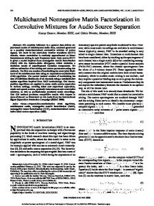
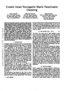
There are two simulations in this example. In the first simulation, n is fixed to be 10. A loop containing 15 experiments is carried out, each of the 15 experiments contains 1000 linear programming computations. In each of the 1000 linear programming computations of the first loop experiment, the non-negative mixing matrix A and the non-negative source vector s0 vector are taken randomly, however, s0 has only one positive component. After the 1000 optimizations, the ratio that the source vectors are estimated correctly is calculated. The k-th loop experiment is carried out similarly but the nonnegative source vector has only k nonzero random entries. The first subplot of Fig. 1 shows the curve of the ratios that the source vectors are estimated correctly obtained in a loop of 15 different experiments. We can see that the source can be estimated correctly when k = 1, 2, and the ratio is larger than 0.95 when k ≤ 5. The second simulation contains loop of 11 different experiments. The number k of nonzero entries of the source vectors is fixed to be 5, and the dimension n of mixture vectors changes from 5 to 15. After each experiment which also contains 1000 linear programming computations, the ratio that the source vectors are estimated correctly is calculated. The second subplot of Fig. 1 shows the curve of the ratios. Example 2: Consider the linear mixing model (25), where source matrix S is composed by 10 sparse face images, the non-negative 6 × 10 mixing matrix is taken randomly of which every column is normalized. In Fig. 2, 10 sparse face images are shown in the subplots of the first and second rows, whereas the 6 mixtures are shown in the subplots of the third and fourth rows. Using the algorithm in Section 3, we obtain the estimated 6 × 14 mixing ¯ and the consistent matrix [A, ¯ E], where E is a 6 × 6 matrix denoted as A, unitary matrix. Solving the linear programming problem (4), we obtain 20 outputs of which 15 outputs shown in Figs. 3. Obviously, the first 10 outputs are the recovered sources. 8
0.8
0.8
0.6
0.6
ratio
1
ratio
1
0.4
0.4
0.2
0.2
0
0
5
10
15
0
5
10 n
k
15
Figure 1: The first subplot: ratios of correctly recovered source vectors s as function of the number of nonzero entries in them (the first simulation of Example 1); the second subplot: ratio of correctly recovered source vectors s as a function of the number of observations (the second simulation of Example 1).
Figure 2: The ten subplots in the first two rows: the 10 sparse face images; The six subplots in the third and fourth rows: the six mixtures
6
Concluding remarks
Nonnegative matrix factorization is discussed in this paper. A factorization condition on basis matrix is first proposed. For a given consistent basis matrix, although there exist infinite number of solutions (factorizations) generally, the sparse solution is unique with probability one, which can be obtained by using linear programming algorithm. This paper also presents an algorithm for finding a suboptimal basis matrix. This basis matrix is composed by data cluster centers which can guarantee that the coefficient matrix is very sparse. At last, an application of NMF is proposed for blind sparse source separation with less sensors than sources. Two simulation examples reveal the validity and performance of the algorithm in this paper. Using the approach in this paper, the sparse sources can be recovered even if the sources are overlapped to some degree.
9
Figure 3: The fifteen outputs of which the first ten are recovered sources in Example 2 (it has been assumed that the number of sources is also unknown).
References [1] Lee, D. D. & Seung, H. S. (1999), “Learning the parts of objects by nonnegative matrix factorization”, Nature, Vol. 401, No.21, pp.788-791. [2] Chen, S., Donoho, D. L. & Saunders, M. A. (1998), “Automic decomposition by basis pursuit”, SIAM Journal on Scientific Computing, Vol. 20, No.1, pp. 33-61. [3] Olshausen, B. A. & Field, D. J. (1997), “Sparse coding with an overcomplete basis set: a strategy employed by V1?” Vision Research, Vol. 37, pp.33113325. [4] Murray, J. F. & Delgado, K. K. (2001), “An improved FOCUSS-based learning algorithm for solving blind sparse linear inverse problems”, Conference Record of the 35rd Asilomar Conference on Signals, Systems and Computers (IEEE). [5] Bofill P., Zibulevsky, M. (2001), “Underdetermined Blind Source Separation using Sparse Representations”, Signal Processing, Vol.81, No 11, pp.23532362. [6] Zibulevsky, M., Kisilev, P., Zeevi, Y. Y., Pearlmutter, B. A. (2000), “Blind source separation via multinode sparse representation”, NIPS-2001. [7] Zibulevsky, M., Pearlmutter, B. A., Boll, P., & Kisilev, P. (2000), “Blind source separation by sparse decomposition in a signal dictionary”, in Roberts, S. J. and Everson, R. M. (Ed.), Independent Components Analysis: Princeiples and Practice, Cambridge University Press. [8] Lee, T. W., Lewicki, M. S., Girolami, M. & Sejnowski, T. J. (1999), “Blind source separation of more sources than mixtures using overcomplete representations”, IEEE Signal Processing Letter, Vol.6, No. 4, pp. 87-90. [9] Li, Y., Wang, J., Zurada, J. M. (2000), “Blind extraction of singularly mixed sources signals”, IEEE Trans. On Neural Networks, Vol.11, No.6, pp. 1413-1422. 10
[10] Li, Y., Wang, J. (2002), “Sequential blind extraction of linearly mixed sources”, IEEE Trans. On Signal Processing, Vol.50, No. 5, pp. 997-1007.
11