THE INTERNATIONAL JOURNAL OF MEDICAL ROBOTICS AND COMPUTER ASSISTED SURGERY Int J Med Robotics Comput Assist Surg (2012) Published online in Wiley Online Library (wileyonlinelibrary.com) DOI: 10.1002/rcs.1427
ORIGINAL ARTICLE
Non-orthogonal tool/flange and robot/world calibration Floris Ernst1,2* Lars Richter1,3 Lars Matthäus4 Volker Martens1 Ralf Bruder1 Alexander Schlaefer3,5 Achim Schweikard1 1
Institute for Robotics and Cognitive Systems, University of Lübeck, Ratzeburger Allee 160, 23538, Lübeck, Germany
2
HotSwap Lübeck GmbH, 23554, Lübeck, Germany
3
Graduate School for Computing in Medicine and Life Sciences, University of Lübeck, 23538, Lübeck, Germany
4
Eemagine Medical Imaging Solutions GmbH, 10243, Berlin, Germany
Abstract Background For many robot-assisted medical applications, it is necessary to accurately compute the relation between the robot’s coordinate system and the coordinate system of a localisation or tracking device. Today, this is typically carried out using hand-eye calibration methods like those proposed by Tsai/Lenz or Daniilidis. Methods We present a new method for simultaneous tool/flange and robot/ world calibration by estimating a solution to the matrix equation AX = YB. It is computed using a least-squares approach. Because real robots and localisation are all afflicted by errors, our approach allows for non-orthogonal matrices, partially compensating for imperfect calibration of the robot or localisation device. We also introduce a new method where full robot/world and partial tool/flange calibration is possible by using localisation devices providing less than six degrees of freedom (DOFs). The methods are evaluated on simulation data and on real-world measurements from optical and magnetical tracking devices, volumetric ultrasound providing 3-DOF data, and a surface laser scanning device. We compare our methods with two classical approaches: the method by Tsai/Lenz and the method by Daniilidis.
5
Medical Robotics Group, University of Lübeck, 23538, Lübeck, Germany *Correspondence to: F. Ernst, Institute for Robotics and Cognitive Systems, University of Lübeck, Ratzeburger Allee 160, 23538 Lübeck, Germany. E-mail:
[email protected]
Results In all experiments, the new algorithms outperform the classical methods in terms of translational accuracy by up to 80% and perform similarly in terms of rotational accuracy. Additionally, the methods are shown to be stable: the number of calibration stations used has far less influence on calibration quality than for the classical methods. Conclusion Our work shows that the new method can be used for estimating the relationship between the robot’s and the localisation device’s coordinate systems. The new method can also be used for deficient systems providing only 3-DOF data, and it can be employed in real-time scenarios because of its speed. Copyright © 2012 John Wiley & Sons, Ltd. Keywords hand-eye calibration; calibration and identification; medical robots and systems
Introduction
Accepted: 30 January 2012
Copyright © 2012 John Wiley & Sons, Ltd.
Tool/flange (or, equivalently, hand-eye or eye-in-hand calibration) and robot/ world calibration is an important topic whenever it comes to a machine interacting with objects detected by some sort of camera, tracking system or other localisation device. In general, tool/flange and robot/world calibration boils down to solving a matrix equation of the type AX = YB (simultaneous tool/flange and robot/world calibration), where the matrices A and B are known and the matrices
F. Ernst et al.
X and Y are unknown. Typically, A would be the pose matrix of a robot and B would be the position and orientation of a calibration object with respect to a tracking device. Consequently, the matrix X is the flange/tool matrix and Y is the robot/world matrix. This problem is usually tackled by taking measurements at multiple stations (A, B)i and eliminating one of the two unknown matrices to arrive at the sim!1 plified equation A!1 j Ai X ¼ XBj Bi. The first works on solving this solution were devised independently by Shiu and Ahmad (27,28) and Tsai and Lenz (30,31). Both solutions make use of matrix algebra and the special properties of homogeneous matrices, separately determining the rotational and translational parts of the matrix X. An early review of these methods was given in (32), where the algorithm by Tsai and Lenz performed slightly better than the algorithm by Shiu and Ahmad. Other works, which also compute these components separately, are on the basis of quaternion algebra (7), screw motion analysis (5), the properties of the Euclidean group (21) and the solution of nonlinear equations (9,11,12). Li and Betsis (17) compare their methods by using a geometric approach, a least-squares solution, and a nonlinear optimisation problem to the methods presented in (31) and (11). Again, the algorithm by Tsai and Lenz proved to be best and as good as their new nonlinear optimisation method. Interest was also sparked to simultaneously compute the rotational and translational parts. This was carried out in (8) by a dual quaternion approach, in (36) and (35) by a one-stage iterative method minimising a nonlinear cost function, in (22) by nonlinear minimisation of a sum of scalar products and in (29) by means of parameterisation of a stochastic model. In (38), the approach from (28) was extended to quaternion algebra (37) and used to simultaneously compute the parameters of the matrices X and Y. In (39), solving the hand-eye calibration problem is coupled with calibrating the robot’s kinematic parameters and the camera’s intrinsic parameters, resulting in a very large (up to 32 parameters) nonlinear optimisation problem. In (1), the authors refrain from using a calibration rig and attempt to solve the calibration problem by means of a structurefrom-motion approach. All those methods, however, have one thing in common: they expect that orthogonal homogeneous matrices1 X and Y can be found which optimally solve the relation AX = YB. In reality, however, this is not necessarily the case: a typical robot will not be calibrated perfectly. Also, for new industrial robots deviations up to 2 ! 3 mm can arise (2). Neither will an arbitrary tracking device deliver results that are exact. Optimal calibrated optical tracking systems will have a root mean square (RMS) error of 0.2 ! 0.3 mm (34). For electromagnetic tracking systems, RMS errors of 1 ! 1.5 mm can arise (10). The expected tracking accuracy for non-common tracking systems, used in medical applications, like 4D Ultrasound or 3D laser scanning systems is # 0.5 and # 1 ! 1.5 mm, respectively.
1 In this work, the terms orthogonal matrix and orthonormalisation only refer to the upper left 3 $ 3-submatrix of a 4 $ 4 homogeneous matrix.
Copyright © 2012 John Wiley & Sons, Ltd.
In many medical applications, robots have become an important component and are required in many cases. For Transcranial Magnetic Stimulation (TMS), for instance, robotized systems are requested for precise and repeatable coil positioning on the head (16). A current development of a robot based system for TMS consists of an industrial robot for coil placement and a stereo-optical infrared tracking system for navigation (19). As for brain stimulation, only a small part of the robot workspace is used, local accuracy is more important. In particular, robot/world calibration algorithms should be adapted for robust real time calibration for robotized TMS (26). Laser scanning systems are used for motion detection and patient registration in medical applications (14). In literature, it has been proposed to use a 3D laser scanning system to track human faces (15) and devices such as the GateRT system (VisionRT, London, UK) are used to detect a patient’s respiratory phase by tracking his/her chest. In general, laser scanning can also be used as a generic tracking device, especially suited for direct tracking, that is, when it is desirable that a target can be tracked without the need for attaching a marker. The laser scanning system directly scans the target and provides a 3D surface of the object. Even though accuracy of laser scanning systems is not as high as of stereo-optical infrared system, these systems can become a convenient alternative to standard tracking devices for medical robotic scenarios (25). A relatively new tracking method, proposed in (3), makes use of a high-speed ultrasound station (GE Vivid7 Dimension, GE Healthcare, Little Chalfont, UK). It has been extended with tracking capabilities and can be used to locate a target volume by template matching or maximum intensity search up to 60 times per second. Combined with an industrial robot, the system is used for real time target tracking in radiotherapy (4). Furthermore, ultrasound is used for a laparoscopic liver surgery assistant system (18). To take this into account, and to also allow for more freedom in the tracking modality used, we propose to extend tool/flange and robot/world calibration to allow non-orthogonal matrices, that is, to try to correct for system inaccuracies in the tool/flange and robot/world calibration matrices. It is also important that all calibration algorithms (except for (1), which requires a scene with more than one distinct feature) rely on matrices describing the full six degree of freedom (DOF) pose of a calibration rig in space. Consequently, tracking devices delivering information with less than six DOFs cannot be used. In this work, we will present a new method with three different variations on the basis of a naïve least-squares solution of the equation system AX = YB (for simultaneous tool/flange and robot/world calibration). This approach combines the following important features: • Because we deal with real-world localisation devices and imperfect robots, we allow the matrices X and Y to be non-orthogonal. Int J Med Robotics Comput Assist Surg (2012) DOI: 10.1002/rcs
Non-orthogonal tool/flange and robot/world calibration for realistic tracking scenarios in medical applications
• The methods compute simultaneously the rotational and translational parts of the matrices X and Y. • As calibration is not necessarily required for the full robot workspace for many medical applications, the algorithm aims for high local accuracy (i.e. required in (20)). • In the case of deficient tracking data, a partial solution is presented, that is, when the localisation device only provides translational data or does not provide full rotational data.
Mi X ! YNi ¼ 0;
i ¼ 1; . . . ; n:
(3)
By regarding the non-trivial elements of X and Y as components of a vector # $T w ¼ x1;1 ; x2;1 ; . . . ; x3;4 ; y1;1 ; y2;1 ; . . . ; y3;4 2 R24 ; Equation 3 can be combined into a system of linear equations Aw ¼ b;
Methods
where A 2 R
Tool/flange and robot/world calibration First, the novel non-orthogonal calibration method is presented for tracking data providing full six DOF. Later, an adaptation of the method for tracking data with only partial tracking information having less than six DOF is described. The last variation deals with preconditioning of the equation system. Non-orthogonal calibration A naïve approach to tool/flange and robot/world calibration is to look at the general relation R
TE E TM ¼R TT T TM ;
(1)
12n$24
(4)
12n
and b 2 R . More specifically, 2 3 2 3 A1 b1 6 A2 7 6 b2 7 7 6 6 A ¼ 4 5 and b ¼ 4 7 ; ⋮ ⋮5 An bn
where the matrices Ai 2 R12$24 and the vectors bi 2 R12 are determined as shown in Equation 6. 2
R½Mi +ðNi Þ1;1 R½Mi +ðNi Þ2;1 6 R½Mi +ðNi Þ1;2 R½Mi +ðNi Þ2;2 Ai ¼6 4 R½Mi +ðNi Þ1;3 R½Mi +ðNi Þ2;3 R½Mi +ðNi Þ1;4 R½Mi +ðNi Þ2;4 + , Z9$1 and bi ¼ !T ½Mi +
R½Mi +ðNi Þ3;1 R½Mi +ðNi Þ3;2 R½Mi +ðNi Þ3;3 R½Mi +ðNi Þ3;4
Typically, the robot’s end effector is moved to random points selected from inside a sphere with radius r. Additionally, a random rotation of up to % d degrees in yaw, pitch and roll is added to the pose. As a shorthand, let Mi ¼ ðR TE Þi , X¼E TM , Ni ¼ ðT TM Þi and Y¼R TT . Consequently, Equation 2 can be written as
3 Z3$3 7 Z3$3 ! E127 5 Z3$3 R½Mi + (6)
E
which is illustrated in Figure 1. Here, the matrices TM , the transform from the robot’s end effector to the marker, and R TT , the transform from the robot’s base to the tracking system are unknown. To compute these matrices, n measurements for different robot poses are taken, resulting in n equations !R " E ! " TE i TM ¼R TT T TM i ; i ¼ 1; . . . ; n: (2)
(5)
Here, R½Mi + 2 R3$3 is the rotational part of Mi, T ½Mi + 2 R is the translational part of Mi, Zm $ n is the m $ n zero matrix and Ek is the k $ k identity matrix. This system can then be solved in a least squares sense by means of QR-factorisation. The resulting vector w now contains the non-trivial entries of the matrices X and Y. Note that this method tries to find the optimal entries for X and Y in terms of the quadratic error, that is, it minimises 3
n X
kMi X ! YNi kF ;
(7)
i¼1
whence the resulting matrices are not necessarily orthogonal. Here, ‖ . ‖F is the Frobenius norm. We call this method the QR24 calibration algorithm because 24
Figure 1. Principles of tool/flange and robot/world calibration: A marker M is attached to the robot’s end effector E and measured by the tracking system or an ultrasound station T. Tool/flange and robot/world calibration is used to determine the unknown transforms R TT , the transform from the robot’s base to the tracking system, and E TM , the transform from the end effector’s local system to the marker’s local system Copyright © 2012 John Wiley & Sons, Ltd.
Int J Med Robotics Comput Assist Surg (2012) DOI: 10.1002/rcs
F. Ernst et al.
elements have to be estimated, and QR-factorisation is used for solving the equation system. Note that, the QR24 algorithm solves for 24 parameters instead of 12 parameters used by standard calibration approaches. As we consider inaccuracies by tracking and robot in the calibration, shearing and scaling can occur in the matrices besides rotation and translation. Thus, the QR24 calibration problem is not over-parameterized when using non-orthogonality. Calibration using only partial tracking information In some situations, the tracking system might not deliver full 6-DOF poses. This will happen whenever the tracking system does not determine the pose of a rigid body but the location of one point in space, such as the position of one light-emitting diode (LED) or the position of maximum intensity in a US volume or the probe does not provide full rotational information. For instance, NDI’s 5-DOF magnetic sensors (Northern Digital Inc., Waterloo, Ontario, Canada) do not provide information about the roll angle. In such cases, the classical calibration algorithms such as the ones presented in (31) and (8) cannot be used. The QR24 calibration algorithm, however, can be adapted to deal with these partial measurements. A closer look at Equation 3 shows that it can be written as shown in Equation 8.
+
the calibration results obtained using inches, metres or millimetres. We have thus extended the QR24 algorithm to allow for an arbitrary scaling factor of the translation. We have performed all experiments with translational values given in mm. Additionally, we used a scaling factor of 0.001 in a second run of the QR24 algorithm to demonstrate the effect of preconditioning (these results are denoted with QR24M).
Orthonormalisation Because—as described earlier—X and Y do not need to be orthogonal during computation, poses calibrated using these matrices must be orthonormalised for the final result. Otherwise, rigid body transformations by using the found calibration matrices would not be applicable. To avoid the bias incurred by Gram–Schmidt orthonormalisation, we propose to use orthonormalisation by means of singular value decomposition (SVD). To this end, let us assume that N is a pose measured by the tracking system, and we want to know this pose in robot coordinates. We then compute YN, a non-orthogonal matrix, and subsequently determine the ‘closest’ orthogonal matrix,
, + , + , + , R½X+ T ½X+ R½Ni + T ½Ni + R½Mi + T ½Mi + R½Y + T ½Y + ! ¼ Z1$3 Z1$3 1 1 1 Z1$3 1 , Z1$3 + R½Mi +R½X+ ! R½Y +R½Ni + R½Mi +T ½X+ þ T ½Mi + ! R½Y +T ½Ni + ! T ½Y + ¼ ¼ Z1$3 0 ¼ Z4$4 :
Using only the upper right part of this matrix equation, R½Mi +T ½X+ þ T ½Mi + ! R½Y +T ½Ni + ! T ½Y + ¼ Z3$1 ;
(8)
(YN)⊥. Let UΣVT = YN be the SVD of YN. Then (YN)⊥ can be computed as UVT. 2
(9)
shows that we can determine Y and T ½X+ by only using T ½Ni + and Mi, that is, without using rotational information from the tracking system. Consequently, the matrices Ai and the vectors bi from Equation 6 are changed as shown in Equation 10.
Computing calibration errors
Using the calibration matrices R TT and E TM, computed by any calibration method, we can determine the calibration quality by looking at Equation 1. In the situation of perfect i calibration, this equation can be transformed to
h Ai ¼ R½Mi +ðNi Þ1;4 R½Mi +ðNi Þ2;4 R½Mi +ðNi Þ3;4 R½Mi + ! E3 and bi ¼ !T ½Mi + (10) This method is called the QR15 calibration algorithm because we can estimate only 15 elements.
Preconditioning the equation system One drawback of the QR24 algorithm is its sensitivity with respect to the unit of the translational component of the pose matrices: all elements of X and Y are treated equally, that is, errors in the rotational part are treated with the same importance as errors in the translational part. Consequently, there will be a difference between Copyright © 2012 John Wiley & Sons, Ltd.
!E
TM
"!1 !R
TE
"!1 R
TT T TM ¼ E4 :
(11)
Note that in reality, equality in Equation 1 will not hold, and, consequently, deriving Equation 11 is not frameinvariant: there are eight possible ways of expressing this relation. Because all frames of reference are equally valid, it has been proposed in literature (29) to use the average of the errors from all possible frames of reference. But when the tracking system does not deliver full 6-DOF measurements, the matrices E TM and R TT cannot be 2 Note that we do not actually perform orthonormalisation of YN but of R½YN +. See also footnote 1.
Int J Med Robotics Comput Assist Surg (2012) DOI: 10.1002/rcs
Non-orthogonal tool/flange and robot/world calibration for realistic tracking scenarios in medical applications
inverted. Consequently, we have to use Equation 11 for 6-DOF data and the following equation for 3-DOF data to ensure comparable results: !R "!1 R # $ # $ TE TT T T TM ! T E TM ¼ Z3$1 : (12) To determine calibration quality, we introduce the following measures: • Translational accuracy and • rotational accuracy. 0 1⊥ !1 !1 Let A ¼ ðE TM Þ ðR TE Þ R TT T TM . Then its transla-
tional error is defined as qffiffiffiffiffiffiffiffiffiffiffiffiffiffiffiffiffiffiffiffiffiffiffiffiffiffiffiffiffiffiffiffiffiffiffiffi etrans ½A+ ¼ A21;4 þ A22;4 þ A23;4 :
(13)
To determine the rotational accuracy, let (k, θ) be the axis-angle representation of R½A+. Then the rotation error is defined as erot ½A+ ¼ jθ j:
% [500, 2000] mm. Using these matrices, 500 completely random orthogonal robot poses Mi were generated and, subsequently, the corresponding tracking matrices Ni were computed. To simulate the actual behaviour of an optical tracking system, a tool with four markers was defined as 3 2 0 50 50 0 6 0 0 50 50 7 7: tool ¼ 6 40 0 0 0 5 1 1 1 1 e i , the To determine the distorted tracking matrices N tool was moved to the pose described by Ni, and the e i was computed as the best fit computed by matrix N Horn’s algorithm without scaling (13), that is,
Here,
2
si;1;1 6 si;2;1 6 Σi ¼ 4 si;3;1 0
(14)
In this metric (as was carried out in (29), where more details can be found), we regard the axis of rotation as irrelevant. Clearly, this approach is only possible if both calibration matrices R TT and E TM as well as 6-DOF tracking information is available. If the tracking system only delivers 3-DOF or 5-DOF information, we cannot compute the rotation errors, and the formula for computation of the translation error is changed to qffiffiffiffiffiffiffiffiffiffiffiffiffiffiffiffiffiffiffiffiffiffiffiffiffiffi etrans ½a+ ¼ a21 þ a22 þ a23 ; (15) where
e i ¼ hornðtool; Ni .tool þ Σi Þ: N si;1;2 si;2;2 si;3;2 0
si;1;3 si;2;3 si;3;3 0
3 si;1;4 si;2;4 7 7 si;3;4 5 0
and si, j, k were drawn from the Gaussian process with s = 0.05 mm. The robot matrices were distorted in a different way: their rotational part was disturbed by multiplication with a random rotation matrix around an arbitrary axis ai. The rotation angles θi were selected from the Gaussian distribution with s = 0.051 , and their translational part was disturbed by additive Gaussian noise: + , e i ¼ R½Mi +.rotai ðθ i Þ T ½Mi + þ Σi ; M 0 1 where
a¼
!R
TE
"!1 R
TT T
#T
$
TM ! T
#E
$ TM :
(16)
Experimental validation—collecting data To evaluate the accuracy and robustness of the proposed calibration methods, we have performed multiple calibration tests. In the first test, simulated data were used. In the second test, calibration was performed using four real world set-ups as shown in Figure 2 and using the algorithm of Tsai and Lenz, Daniilidis’ dual quaternion method as well as the new methods proposed. The robot was controlled using our robot client/server framework, presented in (24). Computer-generated data To test the calibration algorithms, random orthogonal matrices X and Y were generated. To create realistic values, the elements of T ½X+ were selected randomly from [!20, 20] mm, and the elements of T ½Y + from Copyright © 2012 John Wiley & Sons, Ltd.
# $T Σi ¼ si;1 ; si;2 ; si;3
and si, k were drawn from the Gaussian process with s = 0.05 mm. Data from tracking systems Real data were generated using two tracking systems: an optical device and a magnetic tracking system (NDI’s Polaris Spectra and Aurora systems, Northern Digital Inc., Waterloo, Ontario, Canada). Both systems are capable of delivering full 6-DOF tracking data. Optical tracking The spectra system was mounted to a KUKA KR 16 robot (KUKA Roboter GmbH, Augsburg, Germany), and an active 4-LED marker was attached to the end effector of an Adept Viper s850 robot (Adept Technology, Inc., Livermore, California) (Figure 2(a)). The marker and the camera were positioned such that the marker’s tracked position was in the centre of the camera’s working volume (in this case, at x = 0, y = 0 and z = ! 1500 mm). Subsequently, the marker was moved to 500 poses around the initial pose P0. These poses were determined by Int J Med Robotics Comput Assist Surg (2012) DOI: 10.1002/rcs
F. Ernst et al.
Figure 2. Set-up of the calibration experiment. (a) shows the optical tracking camera mounted to a KUKA KR16 robot and optical marker attached to an Adept Viper s850 robot; (b) shows the magnetic tracking system on a plastic table and the magnetic sensors attached to an acrylic bar carried by the Adept robot; (c) shows the LAP GALAXY laser scanner and the calibration phantom carried by the Adept robot; and (d) shows the ultrasonic probe and the lead ball phantom mounted to the Adept robot
Pi ¼ P0 TðtÞRX ðθ 1 ÞRY ðθ 2 ÞRZ ðθ 3 Þ; i ¼ 1; . . . ; 500;
(17)
where Ra(θ) is a rotation matrix around the a-axis by θ, and T is a translation matrix with translation vector t. t and θj, j = 1, . . ., 3, were selected randomly for each pose Pi such that ‖t‖ ≤ r and |θj| ≤ θmax. r was selected as 100 mm, and θmax was selected as 101 . At each calibration station, 100 measurements were averaged to reduce the error from possible robot jitter and sensor noise. Magnetic tracking The values of the magnetic test were generated similarly: the field generator was placed on a plastic table, and a 6-DOF sensor coil was attached to an acrylic plate (1 m long) that was attached to the robot’s end effector (Figure 2 (b)). Using this set-up, 500 pose pairs were collected with r set to 75 mm and θmax set to 51 . Again, 100 measurements were averaged at each calibration station.
Other modalities To determine the applicability of the calibration algorithms to other, less common, imaging/tracking modalities, we have also collected data by using a 3D laser scanning system (LAP GALAXY) and a 4D ultrasound station (GE Vivid7 Dimension). Laser scanning In our case, we used the LAP GALAXY system (LAP Laser Applikationen GmbH, Lüneburg, Germany) and attached Copyright © 2012 John Wiley & Sons, Ltd.
a special calibration tool to the robot. This tool is then scanned with the laser scanning system. To determine its pose, the calibration tool is measured relatively to a reference image. The pose matrices determined can be used with the proposed calibration methods (23). Using the laser scanner is not as simple as using an offthe-shelf tracking system. It is time consuming to collect a large set of data points for calibration. This is because a special calibration tool has to be used as a marker, and the laser scanning system does not directly provide the pose matrix of the tool. To determine its pose, we require a reference image of the calibration tool. Then the pose matrix, relating the actual position and orientation of the scanned tool to the reference image, can be computed with, for example, an iterative closest point (ICP) algorithm (6). This indirect approach is necessary because the laser scanning system only provides a point cloud of the measured surface. Figure 3 shows the MATLAB graphical user interface (The Mathworks, Natick, MA, USA) used for landmark-based preregistration and ICP registration as well as a typical result. Consequently, we have used a set of only n = 50 randomly distributed data points to test calibration of the laser scanning system. Figure 2(c) shows the set-up used to collect the data. Ultrasound We have used a simple lead ball phantom, moved by the robot, to calibrate the robot’s coordinate system to the coordinate system of the ultrasonic head. Note that this Int J Med Robotics Comput Assist Surg (2012) DOI: 10.1002/rcs
Non-orthogonal tool/flange and robot/world calibration for realistic tracking scenarios in medical applications
ICP−based registration
Landmark−based registration
150
150
100
100
50
50 0 −100
0 −100 −200
−200 target surface
0 −100 −200
0 −100 −200
model surface
Figure 3. Registration process used for laser scanner calibration
approach will result in 3-DOF data. Using the same approach, it would also be possible to calibrate the probe with respect to an optical marker tracked by an optical tracking system. It must be noted that, because of varying speeds of sound in different tissues, calibration in a water tank must result in a non-unity scaling factor (this factor should be about 0.96, because the speed of sound in water is 1480 m/s and, on average, 1540 m/s in human tissue). Tracking the lead ball was performed using a maximum intensity algorithm running directly on the ultrasound machine. The data (500 pose pairs) were acquired in the same way as for the optical and magnetic tracking systems. Because of the limited field of view of the ultrasound probe, however, r was set to 15 mm, and θmax was set to 31 . Figure 2(d) shows the set-up used. To allow sub-voxel tracking, not the voxel with maximum intensity but the position in space corresponding to the centre of mass of the tracked object was used. This position was determined by fitting a quadratic polynomial to the intensities of the voxels around the brightest voxel and using this polynomial’s extremal value as tracked position. By using this method, an accuracy of better than 0.5 mm can be achieved throughout the volume. Copyright © 2012 John Wiley & Sons, Ltd.
Results Evaluation speed and implementation Evaluation of the algorithms was carried out on a standard business notebook (Intel Core i5-2540 M CPU with 8 GB of RAM, running Windows 7 $ 64). The algorithms were all implemented in MATLAB R2011a. Sample evaluation times for the algorithms are less than 0.1 s for the QR24, QR15 and Tsai–Lenz methods and below 0.5 s for the dual quaternion method. The methods by Tsai–Lenz and the dual quaternion method were taken from (33).
Calibration errors To compare the quality of the calibration algorithms, calibration was performed using the poses P1, . . ., Pn for n = 5, . . ., 250. For all such cases, the determined calibration matrices were evaluated using the remaining poses P251, . . ., P500. The rotation and translation errors were computed for each testing pose, and the average of all 250 testing poses was determined. Figure 4 shows these Int J Med Robotics Comput Assist Surg (2012) DOI: 10.1002/rcs
F. Ernst et al. Tsai−Lenz
Dual Quaternion
QR24
average calibration error [°]
0.6
0.4
0.2 100
150
200
0.132
0.13
0.128
0.126
250
50
100
150
200
250
number of pose pairs used in calibration
number of pose pairs used in calibration
translation errors, magnetic tracking
rotation errors, magnetic tracking
2
1.5
1
0.5 50
100
150
200
250
0.28 0.26 0.24 0.22 0.2 0.18 50
number of pose pairs used in calibration translation errors, synthetic data
0.5 0.4 0.3 0.2 0.1 100
150
200
150
200
250
rotation errors, synthetic data
0.6
50
100
number of pose pairs used in calibration average calibration error [°]
average calibration error [mm]
true matrices
rotation errors, optical tracking
average calibration error [°]
average calibration error [mm]
average calibration error [mm]
translation errors, optical tracking 0.8
50
QR24M
QR15
250
number of pose pairs used in calibration
0.11
0.105
0.1
0.095
50
100
150
200
250
number of pose pairs used in calibration
Figure 4. Calibration errors for the QR, Tsai–Lenz, and dual quaternion algorithms. The algorithms used n = 5, . . ., 250 poses to compute the calibration matrices that were then tested on 250 other poses. The top graphs show the mean errors by using optical tracking, the centre graphs show the mean errors by using magnetic tracking and the bottom graphs show the mean errors by using simulated data. In the bottom graphs, the turquoise lines show the calibration errors obtained using the correct matrices X and Y. Note that, for the translation errors, the results for the QR24 and QR15 algorithms are nearly identical, whence the corresponding lines coincide
averages for the optical set-up (top), the magnetic set-up (centre) and the simulated data (bottom). We can clearly see that using more than about 50 poses hardly influences the translational error of the QR24 and QR15 algorithms in all three experiments. Even more, their errors are lowest by far (approximately 0.09 mm for the optical system, 0.27 mm for the magnetic system and 0.123 mm for the simulated data). On the synthetic data, we can see that the resulting error comes very close to the error obtained using the correct matrices. It remains within 1%. When looking at the rotational errors, however, the picture is somewhat different: the dual quaternion algorithm performs best on the real data but all algorithms perform similarly on the simulated data. The difference, however, is not as pronounced as for the translational errors. When using the scaled method (i.e. QR24M), we can see that we gain rotational accuracy at the expense of higher translational errors, with results comparable with the dual quaternion algorithm. Very interesting, however, is that calibrating using more pose pairs does not necessarily result in improved results for Copyright © 2012 John Wiley & Sons, Ltd.
all algorithms. This can be seen most clearly for the translational error of the Tsai–Lenz algorithm when using data from optical tracking. Additionally, Table 1 shows the statistics of the errors for the optical and magnetic tests obtained using the optimal matrices, that is, those matrices resulting in minimal RMS error on the test poses. In Figure 5, the results of the optical tracking system are visualised. Again, the QR-based algorithms clearly outperform the dual quaternion and Tsai–Lenz methods. Other modalities For the other two modalities described before, laser scanning and volumetric ultrasound, the proposed calibration algorithms perform very satisfactorily. Laser scanner: For the data collected with our laser scanning system, the results are given in Table 2(a) and Figures 6 and 7. It is clear that, in terms of translational accuracy, the proposed methods strongly outperform the algorithms by Tsai and Lenz and the Dual Quaternion method: the improvement in Int J Med Robotics Comput Assist Surg (2012) DOI: 10.1002/rcs
Non-orthogonal tool/flange and robot/world calibration for realistic tracking scenarios in medical applications Table 1. Error statistics of the calibration algorithms using optimal matrices on the test data (a) Optical tracking system. Optimal values were obtained for n = 5 pose pairs for the Tsai–Lenz algorithm, n = 221 for the dual quaternion algorithm, n = 14 for the QR24M algorithm and n = 229 for the QR24 and QR15 algorithms. Algorithm
Min
25th p
Tsai–Lenz Dual quaternion QR24M QR24 QR15
0.0350 0.0156 0.0388 0.0223 0.0223
0.2112 0.1610 0.1685 0.0923 0.0920
Tsai–Lenz Dual quaternion QR24M QR24 QR15
0.0042 0.0072 0.0117 0.0130 —
0.0625 0.0586 0.0666 0.0627 —
Median Translation error (mm) 0.2950 0.2239 0.2255 0.1317 0.1314 Rotation error (1 ) 0.0979 0.0857 0.0961 0.0940 —
75th p
Max
0.4101 0.3625 0.3253 0.1792 0.1790
0.9289 0.8305 0.6833 0.3095 0.3089
0.1312 0.1187 0.1342 0.1270 —
0.3758 0.3832 0.3860 0.4069 —
(b) Magnetic tracking system. Optimal values were obtained for n = 12 pose pairs for the Tsai–Lenz algorithm, n = 25 for the dual quaternion algorithm, n = 8 for the QR24M algorithm and n = 235 for the QR24 and QR15 algorithms. Min
25th p
Tsai–Lenz Dual quaternion QR24M QR24 QR15
0.0237 0.0603 0.0581 0.0124 0.0123
0.3905 0.5985 0.2955 0.1662 0.1652
Tsai–Lenz Dual quaternion QR24M QR24 QR15
0.0253 0.0477 0.0550 0.0401 —
0.1514 0.1336 0.1661 0.1079 —
Median Translation error (mm) 0.5703 0.9406 0.4830 0.2578 0.2561 Rotation error (1 ) 0.2220 0.1802 0.2520 0.1526 —
75th p
Max
0.7627 1.3859 0.7405 0.3566 0.3538
1.4578 2.8085 1.6096 0.8078 0.8057
0.3615 0.2434 0.4059 0.2500 —
1.0087 0.9066 1.1008 0.8965 —
The numbers shown are minimum, 25th percentile, median, 75th percentile and maximum. Minimal values for each column are marked in bold. (a) shows the data for the optical system, (b) for the magnetic system.
0.35
rotation error [°]
translation error [mm]
0.4 0.8
0.6
0.4
0.2
0.3 0.25 0.2 0.15 0.1 0.05
0 Tsai−Lenz DQ
QR24M QR24 QR15
0 Tsai−Lenz DQ
QR24M QR24 QR15
Figure 5. These plots show the translation (left) and rotation (right) errors on the optical test data set by using optimal calibration matrices. The number of pose pairs used was n = 5 for the Tsai–Lenz algorithm, n = 221 for the dual quaternion algorithm, n = 14 for the QR24M algorithm, and n = 229 for the QR24 and QR15 algorithms. The corresponding numbers are given in Table 1(a)
median error is around 80%. The rotation errors are similar for all systems, their median values ranging from 0.81 to 0.951 . One thing, however, is interesting: preconditioning the QR24 algorithm massively decreases translational accuracy while only slightly reducing rotational errors. In general, given the laser scanner’s accuracy of approximately 0.5 mm and the average accuracy of the ICP matching of 1.1 mm, a median translational calibration error of 1.3–1.4 mm is convincing. Ultrasound: By using the pose pairs collected, it was possible to compute the matrices Y and T ½X + . Because the data Copyright © 2012 John Wiley & Sons, Ltd.
recorded from the ultrasound station features only three DOF, the only calibration method we can use is the QR15 algorithm. Again, we computed the calibration matrices by using n = 5, . . ., 250 pose pairs and computed the translational errors on the other 250 pose pairs. We can see from Figure 8 that the error’s start is below 1 mm even when using only five pose pairs and drops to below 0.6 mm when using more than 25 pose pairs. The error eventually stabilises around 0.52 mm. This result is well in line with the expected tracking accuracy of approximately 0.5 mm. Additionally, Figure 8 also shows the distribution of the calibration error amongst the 250 pose pairs used for testing when the Int J Med Robotics Comput Assist Surg (2012) DOI: 10.1002/rcs
F. Ernst et al. Table 2. Error statistics of the calibration algorithms by using optimal matrices on the test data (a) Laser scanner data, see also Figure 7 Translation error (mm) Algorithm
Min
25th p
Tsai–Lenz DQ QR24M QR24 QR15
1.2812 2.0395 4.4768 0.8984 0.8848
4.7987 4.7066 7.7452 1.1740 1.1702
Tsai-Lenz DQ QR24M QR24 QR15
Min 0.2883 0.4873 0.2442 0.4121 —
25th p 0.6180 0.7327 0.6146 0.6702 —
7.6678 6.7426 10.6338 1.3517 1.3216 Rotation error (1 ) Median 0.8088 0.9475 0.8193 0.8574 —
(b) Ultrasound data, see also Figure 8 Translation error (mm) 25th p Median 0.3165 0.4837
Algorithm Min 0.0802
QR15
Median
75th p
Max
10.3164 9.0190 15.7291 2.1678 2.1760
18.1265 13.3181 28.5564 3.3947 3.4044
75th p 0.9393 1.1914 0.9869 1.1523 —
Max 1.4628 1.4691 1.3946 1.4730 —
75th p 0.7023
Max 1.2197
The numbers shown are minimum, 25th percentile, median, 75th percentile and maximum. Minimal values for each column are marked in bold. (a) shows the data from the laser scanner system, (b) shows the data from ultrasound calibration.
Dual Quaternion
QR24
Translation errors on the test data
20
10
0
5
10
15
20
QR15
QR24M
Rotation errors on the test data
30
25
average calibration error [°]
average calibration error [mm]
Tsai−Lenz
2
1.5
1
0.5
5
number of pose pairs used in calibration
10
15
20
25
number of pose pairs used in calibration
Figure 6. Calibration errors for the QR, Tsai–Lenz, and dual quaternion algorithms when using laser scanner data. The algorithms used n = 5, . . ., 25 poses to compute the calibration matrices that were then tested on 25 other poses, showing the mean translational (left) and rotational errors (right)
1.4 1.2
rotation error [°]
translation error [mm]
25 20 15 10 5 0 Tsai−Lenz DQ
1 0.8 0.6 0.4
QR24 QR24M QR15
0.2 Tsai−Lenz DQ
QR24 QR24M QR15
Figure 7. Results of the laser calibration with n = 50 data points, 25 of which were used for both calibration and testing. The left graph shows the translation errors of the laser calibration for the Tsai–Lenz, dual quaternion, QR24, QR24M and QR15 algorithms, respectively, using 25 points for calibration and 25 points for testing. The right graph shows the corresponding rotation errors. The corresponding numbers are given in Table 2(a)
optimal calibration matrix (i.e. the one resulting in the lowest average error) is applied. We can see here that the 75th percentile lies at 0.70 mm, and an error of 1.2 mm is never exceeded. Copyright © 2012 John Wiley & Sons, Ltd.
As expected, a typical calibration matrix does exhibit non-unity scaling factors (for n = 174 pose pairs, the factors are 0.970, 0.969 and 0.978), and the matrix is not completely orthogonal (the angles between the axes Int J Med Robotics Comput Assist Surg (2012) DOI: 10.1002/rcs
mean calibration error [mm]
Non-orthogonal tool/flange and robot/world calibration for realistic tracking scenarios in medical applications 1
1.2
0.9
1
0.8
0.8 0.6
0.7
0.4 0.6
0.2
0.5
50
100 150 200 number of pose pairs used in calibration
250
QR15
Figure 8. Translational calibration errors of the QR15 algorithm applied to 3D ultrasound data (250 test poses). The left plot shows the error as a function of the poses used to determine the calibration matrices, the right plot shows the errors on the test poses obtained using the calibration matrices that result in the smallest average error (n = 174), numbers in Table 2(b)
in Figure 9. Again, we can see that the QR24 and QR15 algorithms converge quickly, stabilising at a translational error of about 0.02 mm on X and Y. The rotational errors show a similar picture: an accuracy of less than 0.01∘ is achieved on both matrices. The dual quaternion and Tsai–Lenz algorithms, however, do not show proper convergence. The errors may increase strongly when more poses are used in the calibration routine. The QR24M algorithm, however, results in higher errors on the matrix Y and similar errors on the matrix X when compared with the QR24 algorithm.
of the coordinate system spanned by the matrix are 90.561 , 90.471 and 90.241 ). This confirms that, in the case of a more complex tracking modality, a more robust calibration algorithm is required. For comparison, when looking at the optimal calibration results (QR24 algorithm) of the spectra system, the scaling factors are 1.0010, 1.0018 and 0.9967, and the matrix’ angles are 90.081 , 90.391 and 90.111.
Convergence properties To determine the convergence properties of the different algorithms, the synthetic data were evaluated again. It is clear from Figure 4, bottom row, that all algorithms seem to converge to the error obtained using the correct calibration matrices (the turquoise lines). Additionally, it was possible to determine if and how fast the algorithms converge to the correct matrices X and Y, which are known in this case. The results are shown
For many medical robotic applications—as already mentioned—the selected workspace sizes are in the desired range. However, to show the quality of our algorithms, we have performed additional calibration experiments with the Polaris Spectra system using
Dual Quaternion
QR24
Rotation errors of Y
0.4 0.3 0.2 0.1 0
50
100
150
200
250
0.06 0.05 0.04 0.03 0.02 0.01 0
50
Translation errors of X 0.4 0.3 0.2 0.1 100
150
200
150
200
250
Rotation errors of X
0.5
50
100
number of pose pairs used in calibration
250
number of pose pairs used in calibration
average calibration error [°]
average calibration error [mm]
number of pose pairs used in calibration
0
QR24M
QR15
Translation errors of Y 0.5
average calibration error [°]
average calibration error [mm]
Tsai−Lenz
Increased workspace sizes
0.06
0.04
0.02
0
50
100
150
200
250
number of pose pairs used in calibration
Figure 9. Convergence properties of the QR, Tsai–Lenz, and dual quaternion algorithms on synthetic data. The graphs show the errors between the calibration matrices X and Y as computed by the respective algorithms and the true matrices. Note that, for the translation errors and the rotation errors of Y, the results for the QR24 and QR15 algorithms are nearly identical, whence the corresponding lines coincide Copyright © 2012 John Wiley & Sons, Ltd.
Int J Med Robotics Comput Assist Surg (2012) DOI: 10.1002/rcs
minimal translational error [mm]
F. Ernst et al. Tsai−Lenz
Dual Quaternion
QR24
QR15
QR24M
1.5
1
0.5
0 100mm, 10°
200mm, 10°
300mm, 20°
400mm, 20°
500mm, 30°
400mm, 20°
500mm, 30°
minimal rotational error [°]
workspace of the calibration experiment 0.35 0.3 0.25 0.2 0.15 0.1 100mm, 10°
200mm, 10°
300mm, 20°
workspace of the calibration experiment
Figure 10. Influence of changes in the size of the calibration workspace on the best calibration result achievable by algorithm. The robot and camera were not moved relative to each other between the measurements
increased workspace sizes. (Note that the Aurora system’s workspace is only marginally larger than the workspace used in the first experiment.) We used the following five experiments with changed workspace sizes: 1 2 3 4 5
r = 100 mm and θ = 10∘, r = 200 mm and θ = 10∘, r = 300 mm and θ = 20∘, r = 400 mm and θ = 20∘ and r = 500 mm and θ = 30∘,
with radius of the workspace r and a maximal rotation angle θ. In all cases, the robot was ordered to acquire 1000 samples, which were successfully recorded in the first two experiments. Because of limitations of feasible joint angles, in the third experiment, 971 measurements, in the fourth experiment, 904 measurements and in the fifth experiment, 784 measurements were collected. Figure 10 displays the found calibration errors for this experiment. Interestingly, the general calibration accuracy remained with increased workspace size. Although the errors slightly increased for all calibration methods, the presented calibration methods (QR24 and QR15) were still best.
Discussion We have presented and evaluated a novel method for tool/flange and robot/world calibration. The method has been validated using simulated data, measured data from optical and magnetic tracking systems, and using data from surface laser scanning and volumetric ultrasound. The results were compared with calibration obtained with standard algorithms such as those by Tsai—Lenz and Daniilidis. Copyright © 2012 John Wiley & Sons, Ltd.
We have shown that, when using synthetic data, all methods perform very well with errors below 0.25 mm and 0.11. This shows that all methods are suitable for typical calibration tasks. In our specific set-up, however, where off-the-shelf tracking systems and robots as well as somewhat uncommon devices for localisation were used, we found that the accuracy of our method was typically 50% better than the accuracy of the standard algorithms. It has to be noted, however, that the new method can only be used when • it is acceptable or required to allow non-orthogonality in the calibration matrix/matrices, and • the calibrated system is used in the same spatial area where calibration was performed. Additionally, we have seen in all tests that calibration using our method comes very close to the accuracy we can expect from the systems: the accuracies of the systems are approximately 0.1 mm (optical tracking3), 0.5 mm (magnetic tracking and volumetric ultrasound) and 1 ! 2 mm (laser scanner data), and the median calibration accuracies are 0.13 mm, 0.26 mm, 0.48 mm and 1.35 mm, respectively. We have shown that our method is well-suited to handle deficient tracking data, that is, to systems that do not deliver full 6-DOF pose data (such as volumetric ultrasound or 5-DOF magnetic sensors). The new calibration algorithm can be used to determine the robot/world calibration matrix even in this case, and it has been shown to be equivalent to the full method providing simultaneous tool/flange and robot/world calibration.
3 Note that we used a relatively small working volume and averaged multiple measurements to achieve this spatial accuracy. Typical accuracy of the device across its full measurement volume is approximately 0.3 mm RMS.
Int J Med Robotics Comput Assist Surg (2012) DOI: 10.1002/rcs
Non-orthogonal tool/flange and robot/world calibration for realistic tracking scenarios in medical applications
Concluding, we can say that for many medical applications, where calibration is not necessarily required for the full workspace of the robot and the need for high local accuracy is paramount, our new methods provide a viable alternative to the classical approaches.
19. 20.
References 1. Andreff N, Horaud R, Espiau B. Robot hand-eye calibration using structure-from-motion. Int J Rob Res 2001; 20(3): 228–248. doi:10.1177/02783640122067372. 2. Beyer L, Wulfsberg J. Practical robot calibration with ROSY. Robotica 2004; 22(05): 505–512, DOI: 10.1017/s026357470400027x, http://journals.cambridge.org/article_S026357470400027X 3. Bruder R, Ernst F, Schlaefer A, Schweikard A. Real-time tracking of the pulmonary veins in 3D ultrasound of the beating heart. In: 51st Annual Meeting of the AAPM, American Association of Physicists in Medicine, Anaheim, CA, USA, Medical Physics, vol 36, 2009; 2804, DOI: 10.1118/1.3182643, URL http://www. aapm.org/meetings/09AM/, tH-C-304A-07 4. Bruder R, Ernst F, Schlaefer A, Schweikard A. A framework for real-time target tracking in radiosurgery using threedimensional ultrasound. In: Proceedings of the 25th International Congress and Exhibition on Computer Assisted Radiology and Surgery (CARS’11). CARS: Berlin, Germany; Int J Comput Assist Radiol Surg 2011; 6: S306–S307, URL http://www.cars-int.org 5. Chen HH. A screw motion approach to uniqueness analysis of head-eye geometry. In: Proc. CVPR’91. IEEE Computer Society Conf Computer Vision and Pattern Recognition, 1991; 145–151, DOI: 10.1109/CVPR.1991.139677 6. Chen Y, Medioni G. Object modeling by registration of multiple range images. In: Proc. Conf. IEEE Int Robotics and Automation, 1991; 2724–2729, DOI: 10.1109/robot.1991.132043 7. Chou JCK, Kamel M. Finding the position and orientation of a sensor on a robot manipulator using quaternions. Int J Rob Res 1991; 10(3): 240–254, DOI: 10.1177/027836499101000305, http://ijr.sagepub.com/content/10/3/240.full.pdf+html 8. Daniilidis K. Hand-eye calibration using dual quaternions. Int J Rob Res 1999; 18(3): 286–298. doi:10.1177/02783649922066213. 9. Dornaika F, Horaud R. Simultaneous robot-world and hand-eye calibration. IEEE Trans Rob Autom 1998; 14(4): 617–622. doi:10.1109/70.704233. 10. Frantz DD, Wiles AD, Leis SE, Kirsch SR. Accuracy assessment protocols for electromagnetic tracking systems. Phys Med Biol 2003; 48(14): 2241, URL http://stacks.iop.org/0031-9155/48/ i=14/a=314 11. Horaud R, Dornaika F. Hand eye calibration. In: Workshop on Computer Vision for Space Applications. Antibes, France, 1993; 369–379 12. Horaud R, Dornaika F. Hand-eye calibration. Int J Rob Res 1995; 14(3): 195–210. doi:10.1177/027836499501400301. 13. Horn BKP. Closed-form solution of absolute orientation using unit quaternions. J Opt Soc Am A 1987; 4(4): 629–642. doi:10.1364/JOSAA.4.000629. 14. Juhler-Nøttrup T, Korreman SS, Pedersen AN, Persson GF, Aarup LR, Nyström H, Olsen M, Tarnavski N, Specht L. Interfractional changes in tumour volume and position during entire radiotherapy courses for lung cancer with respiratory gating and image guidance. Acta Oncol 2008; 47(7): 1406–1413, http://informahealthcare. com/doi/pdf/10.1080/02841860802258778 15. Kovacs L, Zimmermann A, Brockmann G, Gühring M, Baurecht H, Papadopulos NA, Schwenzer-Zimmerer K, Sader R, Biemer E, Zeilhofer HF. Three-dimensional recording of the human face with a 3d laser scanner. J Plast Reconstr Aesthet Surg 2006; 59(11): 1193–1202. doi:10.1016/j.bjps.2005.10.025. 16. Langguth B, Kleinjung T, Landgrebe M, de Ridder D, Hajak G. RTMS for the treatment of tinnitus: the role of neuronavigation for coil positioning. Neurophysiol Clin 2010; 40(1): 45–58. 17. Li M, Betsis D. Head-eye calibration. In: Proceedings of the 5th International Conference on Computer Vision (ICCV’95), 1995; 40–45, DOI: 10.1109/ICCV.1995.466809 18. Martens V, Schlichting S, Besirevic A, Kleemann M. LapAssistent - a laparoscopic liver surgery assistence system. In: Proceedings of the 4th European Conference of the
Copyright © 2012 John Wiley & Sons, Ltd.
21. 22.
23.
24.
25.
26.
27.
28.
29.
30.
31.
32. 33. 34.
35. 36.
International Federation for Medical and Biological Engineering, vol 22, Magjarevic R, Sloten J, Verdonck P, Nyssen M, Haueisen J (eds). Springer, IFMBE Proceedings, 2008; 121–125, DOI: 10.1007/978-3-540-89208-3_31 Matthäus L. A robotic assistance system for transcranial magnetic stimulation and its application to motor cortex mapping. PhD thesis, Universität zu Lübeck, 2008 Matthäus L, Trillenberg P, Fadini T, Finke M, Schweikard A. Brain mapping with transcranial magnetic stimulation using a refined correlation ratio and Kendall’s tau. Stat Med 2008; 27(25): 5252–5270. doi:10.1002/sim.3353. Park FC, Martin BJ. Robot sensor calibration: solving AX=XB on the Euclidean group. IEEE Trans Rob Autom 1994; 10(5): 717–721. doi:10.1109/70.326576. Remy S, Dhome M, Lavest JM, Daucher N. Hand-eye calibration. In: Intelligent Robots and Systems, 1997. IROS’97, Proceedings of the 1997 IEEE/RSJ International Conference on, vol 2, 1997; 1057–1065, DOI: 10.1109/iros.1997.655141 Richter L, Bruder R, Schlaefer A, Schweikard A. Towards direct head navigation for robot-guided transcranial magnetic stimulation using 3D laserscans: Idea, setup and feasibility. In: Annual International Conference of the IEEE Engineering in Medicine and Biology Society, IEEE, Buenos Aires, Argentina, vol 32, 2010a; 2283–2286, DOI: 10.1109/IEMBS.2010.5627660 Richter L, Ernst F, Martens V, Matthäus L, Schweikard A. Client/server framework for robot control in medical assistance systems. In: Proceedings of the 24th International Congress and Exhibition on Computer Assisted Radiology and Surgery (CARS’10), CARS: Geneva, Switzerland; Int J Comput Assist Radiol Surg 2010b; 5: 306–307, URL http:// www.cars-int.org/ Richter L, Bruder R, Trillenberg P, Schweikard A. Navigated and robotized transcranial magnetic stimulation based on 3d laser scans. In: Bildverarbeitung für die Medizin, Gesellschaft für Informatik (GI), Informatik akuell, 2011a; 164–168 Richter L, Ernst F, Schlaefer A, Schweikard A. Robust real-time robot-world calibration for robotized transcranial magnetic stimulation. Int J Med Rob Comput Assisted Surg 2011b; 7(4): 414–422. DOI: 10.1002/rcs.411, URL http://dx.doi.org/ 10.1002/rcs.411 Shiu YC, Ahmad S. Finding the mounting position of a sensor by solving a homogeneous transform equation of the form AX = XB. In: Proc. IEEE Int. Conf. Robotics and Automation, IEEE: Raleigh, North Carolina vol 4, 1987; 1666–1671, DOI: 10.1109/ robot.1987.1087758 Shiu YC, Ahmad S. Calibration of wrist-mounted robotic sensors by solving homogeneous transform equations of the form AX=XB. IEEE Trans Rob Autom 1989; 5(1): 16–29. doi:10.1109/70.88014. Strobl KH, Hirzinger G. Optimal hand-eye calibration. In 2006 IEEE/RSJ International Conference on Intelligent Robots and Systems. 2006; 4647–4653. doi:10.1109/ iros.2006.282250. Tsai RY, Lenz RK. A new technique for fully autonomous and efficient 3D robotics hand-eye calibration. In: Proceedings of the 4th international symposium on Robotics Research. MIT Press: Cambridge, MA, USA, 1988; 287–297, URL http:// portal.acm.org/citation.cfm?id=57425.57456 Tsai RY, Lenz RK. A new technique for fully autonomous and efficient 3D robotics hand/eye calibration. IEEE Trans Rob Autom 1989; 5(3): 345–358. doi:10.1109/70.34770. Wang CC. Extrinsic calibration of a vision sensor mounted on a robot. IEEE Trans Rob Autom 1992; 8(2): 161–175. doi:10.1109/70.134271. Wengert C. Hand-eye calibration toolbox for MATLAB. Available online, URL, 2010. http://www.vision.ee.ethz.ch/ software/calibration_toolbox.php. Wiles AD, Thompson DG, Frantz DD. Accuracy assessment and interpretation for optical tracking systems. In: Medical Imaging 2004: Visualization, Image-Guided Procedures, and Display, Galloway RL Jr (ed.) 2004; 5367: 421–432, DOI: 10.1117/12.536128 Zhuang H, Qu Z. A new identification Jacobian for robotic hand/eye calibration. IEEE Trans Syst Man Cybern 1994; 24(8): 1284–1287. doi:10.1109/21.299711. Zhuang H, Shiu YC. A noise tolerant algorithm for wristmounted robotic sensor calibration with or without sensor orientation measurement. In Proc. lEEE/RSJ Int Intelligent
Int J Med Robotics Comput Assist Surg (2012) DOI: 10.1002/rcs
F. Ernst et al. Robots and Systems Conf, Vol. 2. 1992; 1095–1100. doi:10.1109/iros.1992.594526. 37. Zhuang H, Roth ZS, Shiu YC, Ahmad S. Comments on ‘calibration of wrist-mounted robotic sensors by solving homogeneous transform equations of the form AX=XB’ [with reply]. IEEE Trans Rob Autom 1991; 7(6): 877–878. doi:10.1109/70.105398.
Copyright © 2012 John Wiley & Sons, Ltd.
38. Zhuang H, Roth ZS, Sudhakar R. Simultaneous robot/world and tool/flange calibration by solving homogeneous transformation equations of the form AX=YB. IEEE Trans Rob Autom 1994; 10(4): 549–554. doi:10.1109/70.313105. 39. Zhuang H, Wang K, Roth ZS. Simultaneous calibration of a robot and a hand-mounted camera. IEEE Trans Rob Autom 1995; 11(5): 649–660. doi:10.1109/70.466601.
Int J Med Robotics Comput Assist Surg (2012) DOI: 10.1002/rcs