Non-Parametric Estimation of Forecast ... - Monash University

ISSN 1440-771X

Australia

Department of Econometrics and Business Statistics http://www.buseco.monash.edu.au/depts/ebs/pubs/wpapers/

Non-Parametric Estimation of Forecast Distributions in Non-Gaussian, Non-linear State Space Models Jason Ng, Catherine S. Forbes, Gael M. Martin and Brendan P.M. McCabe

September 2011

Working Paper 11/11

Non-Parametric Estimation of Forecast Distributions in Non-Gaussian, Non-linear State Space Models Jason Ngy, Catherine S. Forbesz, Gael M. Martinxand Brendan P.M. McCabe{ August 31, 2011

Abstract The object of this paper is to produce non-parametric maximum likelihood estimates of forecast distributions in a general non-Gaussian, non-linear state space setting. The transition densities that de…ne the evolution of the dynamic state process are represented in parametric form, but the conditional distribution of the non-Gaussian variable is estimated non-parametrically. The …ltering and prediction distributions are estimated via a computationally e¢ cient algorithm that exploits the functional relationship between the observed variable, the state variable and a measurement error with an invariant distribution. Simulation experiments are used to document the accuracy of the non-parametric method relative to both correctly and incorrectly speci…ed parametric alternatives. In an empirical illustration, the method is used to produce sequential estimates of the forecast distribution of realized volatility on the S&P500 stock index during the recent …nancial crisis. A resampling technique for measuring sampling variation in the estimated forecast distributions is also demonstrated. KEYWORDS: Probabilistic Forecasting; Non-Gaussian Time Series; Grid-based Filtering; Penalized Likelihood; Subsampling; Realized Volatility. JEL CODES: C14, C22, C53.

This research has been supported by Australian Research Council (ARC) Discovery Grant DP0985234 and ARC Future Fellowship FT0991045. The authors would like to thank participants at the National PhD Conference in Economics and Business (November, 2010, Australian National University); the 7th International Symposium on Econometric Theory and Applications (April, 2011, Monash University); the International Symposuim of Forecasting (June, 2011, University of Prague); the 8th Workshop on Bayesian Nonparametrics (June, 2011, Veracruz, Mexico); the Australasian Econometric Society Meeting (July, 2011, University of Adelaide); and the Frontiers in Financial Econometrics Workshop (July, 2011, Queensland University of Technology) for constructive comments on earlier drafts of the paper. y Department of Econometrics and Business Statistics, Monash University, Australia. z Department of Econometrics and Business Statistics, Monash University, Australia x Corresponding author: Department of Econometrics and Business Statistics, Monash University, Australia. Email: [email protected]. { Management School, University of Liverpool, UK.

1

1

Introduction

The focus of this paper is on forecasting non-Gaussian time series variables. Such variables are prevalent in the economic and …nance spheres, where deviations from the symmetric bell-shaped Gaussian distribution may arise for a variety of reasons, for example due to the positivity of the variable, to its inherent integer or binary nature, or to the prevalence of values that are far from, or unevenly distributed around, the mean. Against this backdrop, the challenge is to produce forecasts that are coherent - i.e. consistent with any restrictions on the values assumed by the variable - and that also encompass all important distributional information. Point forecasts, based on measures of central tendency, are common. However, they may not be coherent - evidenced, for example, by a real-valued conditional mean forecast of an integer-valued variable. Moreover, such measures convey none of the distributional information that is increasingly important for decision making (e.g. risk management), most notably as concerns the probability of occurrence of extreme outcomes. In contrast, an estimate of the full probability distribution, de…ned explicitly over all possible future values of the random variable is, by its very construction, coherent, as well as re‡ecting all of the important distributional features (including tail features) of the variable in question. Such issues have informed recent work in which distributional forecasts have been produced for speci…c non-Gaussian data types (Freeland and McCabe, 2004; McCabe and Martin, 2005; Bu and McCabe, 2008; Czado et al., 2009; McCabe, Martin and Harris, 2011; Bauwens et al., 2004; Amisano and Giacomini, 2007). In addition, the need to forecast the probability of large …nancial losses has been the primary reason for the recent focus on distributional forecasting of portfolio returns (Diebold et al., 1998; Berkowitz, 2001; Geweke and Amisano, 2010), with this literature, in turn, closely linked to that in which extreme quantiles (or Values at Risk) are the focus of the forecasting exercise (Giacomini and Komunjer, 2005; de Rossi and Harvey, 2009). The extraction of risk-neutral distributional forecasts of non-Gaussian asset returns from derivative prices (Ait-Sahalia and Lo, 1998; Bates, 2000; Lim et al., 2005) is motivated by similar goals; i.e. that deviation from Gaussianity requires attention to be given to the prediction of higher order moments and to future distributional characteristics.1 In the spirit of this evolving literature, we develop a new method for estimating the full forecast distribution of non-Gaussian time series variables. In contrast to the existing literature, in which the focus is almost exclusively on the speci…cation of strict parametric models, a ‡exible non-parametric approach is to be adopted here, with a view to producing distributional forecasts that are not reliant on the complete speci…cation of the true data generating process (DGP). 1

Discussion of the merits of probabilisitic forecasting in general is provided by, amongst others, Dawid (1984), Tay and Wallis (2000), Gneiting et al. (2007) and Gneiting (2008).

2

The method is developed within the general framework of non-Gaussian, non-linear state space models, with the distribution for the observed non-Gaussian variable, conditional on the latent state(s), estimated non-parametrically. The estimated forecast distribution, de…ned by the relevant function of the non-parametric estimate of the conditional distribution, thereby serves as a ‡exible representation of the likely future values of the non-Gaussian variable, given its current and past values, and conditional on the (parametric) dynamic structure imposed by the state space form.2 The recursive …ltering and prediction distributions used both to de…ne the likelihood function and, ultimately, the predictive distribution for the non-Gaussian variable (and for the state also, when of inherent interest), are represented via the numerical solutions of integrals de…ned over the support of the independent and identically distributed (i:i:d:) measurement error - with this support readily approximated in empirical settings. Any standard deterministic integration technique (e.g. rectangular integration, Simpson’s rule) can be used to estimate the relevant integrals. The ordinates of the (unknown) measurement density are estimated as unknown parameters using maximum likelihood (ML) methods, with this aspect drawing on the recent work of Berg et al. (2010) on discrete penalized likelihood (see also Scott et al., 1980; Engle and Gonzalez-Rivera, 1991). The relative computational simplicity of the proposed method - for reasonably low dimensions of the measurement and state variables - is in marked contrast with the high computational burden of the Gaussian sum …lter, an alternative method for avoiding a strict parametric speci…cation for the measurement distribution (see Sorenson and Alspach, 1971; Kitagawa, 1994; Monteiro, 2010). The modest computational burden of the proposed method also stands in contrast with the simulation-based estimation methods needed to implement ‡exible mixture modelling in the non-Gaussian state space realm (e.g. Durham, 2007; Caron et al. 2008; Jensen and Maheu, 2010; Yau, Papaspiliopoulos, Roberts and Holmes, 2010). Extensive simulation exercises are used to assess the predictive accuracy of the non-parametric method, against both correctly speci…ed and misspeci…ed parametric alternatives, and for a variety of DGPs. Assessment of the resulting forecast distributions is based on a range of comparative and evaluative methods including predictive score, probability integral transform and coverage methods. The non-parametric estimation method is then applied to the problem of estimating the forecast distribution of realized volatility for the S&P500 market index during the recent …nancial turmoil. Using the approach developed in McCabe, Martin and Harris (2011), resampling is used to cater for estimation uncertainty in the production of the probabilistic forecasts of volatility. (See also Rodriguez and Ruiz, 2009). 2

Note that the terms ‘forecast distribution’and ‘predictive (or prediction) distribution’are used interchangeably in the paper.

3

The outline of the paper is as follows. In Section 2 we describe the proposed recursive algorithm, with the Dirac delta function ( -function) used to recast all …ltering and predictive densities into integrals de…ned over the constant support of the measurement error. In Section 3.1, we discuss the linear and non-linear models considered in the simulation experiments. In Section 3.2 we then outline the various tools used to compare and evaluate the predictive distributions obtained via the non-parametric and parametric methods, with simulation results then presented in Section 3.3. The empirical application is documented in Section 4, with details given of the subsampling method used to measure the impact of sampling variation on the estimated forecast distribution. Section 5 concludes.

2

Non-parametric Estimation of the Forecast Distribution

2.1

An Outline of the Basic Approach

Our non-parametric estimate of a forecast distribution is developed within the context of a general non-Gaussian, non-linear state space model for a scalar random variable yt : Consider the system governed by a measurement equation for yt and a transition equation for a scalar state variable xt ;

for t = 1; 2; :::; T; where each

t

yt = ht (xt ; t )

(1)

xt = kt (xt 1 ; vt ) ;

(2)

is assumed to be an i:i:d: random variable and the functions

given by ht ( ; ) are assumed to be di¤erentiable with respect to each argument. Further, we assume that, for given values yt and

t,

the function

G (xt ) = yt

ht (xt ; t )

is assumed to have a unique root at xt = xt (yt ; t ) as well as having a non-zero derivative at that root. For the sake of generality we focus on the case where yt is continuous, with all distributions expressed using density functions as a consequence. With simple modi…cations the proposed methodology applies equally to the case of discrete measurements and/or states. Extension to the multivariate setting is also possible, although the simple grid-based method emphasized here is clearly most suitable for reasonably low-dimensional problems. We also focus here on the case where xt (yt ; t ) is analytically available, in addition to being unique, with adaptation of the method obviously required when neither of these conditions are met. As is common, we assume that function (pdf) for

t

t

is independent of xt , in which case the probability density

is simply p ( t jxt ) = p ( t ), for all t = 1; 2; :::; T: We also assume time-series 4

independence for

t;

that is, any dynamic behaviour in yt is captured completely by ht ( ; ) and

kt ( ; ) : However, rather than assume a potentially incorrect parametric speci…cation for p ( t ), we allow its distributional form to be unknown. An initial (parametric) distribution p (x1 ) is speci…ed for the scalar state, with the transition densities resulting from (2) denoted by p (xt jxt 1 ), t = 2; 3; :::; T: In the examples considered in the paper (and as would be standard in many empirical problems), ht ( ; ) and kt ( ; ) are assumed to be known functions for all t; and kt is such that the transition densities p (xt jxt 1 ) are available. To avoid unnecessary notation, we suppress the t subscript on the functions h and k from this point.

Given the model de…ned by (1) and (2), the one-step ahead forecast distribution for yT +1 , conditional on the observed data, y1:T = (y1 ; y2 ; :::; yT )0 , is p (yT +1 jy1:T ) =

Z

p (yT +1 jxT +1 ) p (xT +1 jy1:T ) dxT +1 ;

(3)

where the explicit dependence of p (yT +1 jy1:T ) on any unknown …xed parameters that char-

acterize h ( ; ), p (x1 ), or any of the transition densities fp (xt jxt 1 ) ; t = 2; 3; :::; T g, has been suppressed. The primary aim of the paper is to incorporate, within an overarching ML inferential approach, non-parametric estimation of the conditional measurement distribution, p (yT +1 jxT +1 ), which via (3), will yield a non-parametric estimate of the one-step ahead fore-

cast density, p (yT +1 jy1:T ). In cases where the state variable is also of interest, a non-parametric estimate of the corresponding forecast density for the state, p (xT +1 jy1:T ) ; may be obtained.

As outlined below, the non-parametric method is implemented by representing the unknown density, p (yT +1 jxT +1 ), by its ordinates de…ned, in turn, for N grid points on the support of T +1 :

The nature of these grid-points is determined by the integration method used to estimate

the integrals that de…ne the relevant …ltering/prediction algorithm. This approach introduces an additional N unknown parameters to be estimated (via ML) along with any other unknown parameters that characterize the model. Estimation is subject to the usual restrictions associated with probability distributions and to any restrictions to be imposed on the distribution as a consequence of the role played by xT +1 . A penalty function is used to impose smoothness on the estimated density of yT +1 given xT +1 . Using standard prediction error decomposition, the likelihood function for the collection of all unknown …xed parameters ; augmented, in the current context, by the unknown ordinates of p (yT +1 jxT +1 ), is given by L ( ) / p (y1 )

T Y1 t=1

p (yt+1 jy1:t ) ;

(4)

where y1:t = (y1 ; y2 ; :::; yt )0 : The likelihood function thus requires the availability of the one-step

5

ahead prediction distributions, p (yt+1 jy1:t ) ;

t = 1; 2; :::T

1

(5)

and the marginal distribution p (y1 ) ;

(6)

where both (5) and (6) are (suppressed) functions of : In the following section we outline a computationally e¢ cient …ltering algorithm for computing (5) and (6), needed for the speci…cation of the likelihood function in (4). The unknown parameters are estimated by maximizing the (penalized) likelihood function subject to the smoothness and coherence constraints noted above. Conditional on these estimates, the predictive density in (3) is estimated, with sampling error able to be quanti…ed in empirical settings using resampling methods, as illustrated in Section 4.3. Crucially, the computational burden associated with evaluation of the likelihood function in (4) is shown to be a linear function (only) of the sample size, T: This is in contrast with the computational burden associated with a kernel density representation of p ( t ) ; such as the one used in the Gaussian sum …lter, which is known to be geometric in T (see, for example, Kitagawa, 1994). The computational simplicity of our method derives from the fact that given observed data for period t, the representation of the invariant measurement error density on a common grid implies a variable grid of values for the corresponding state variable, xt . Hence, the computational requirements of evaluating the likelihood using our …lter are equivalent to those that either assume or impose discretization on the state (see, for example, Arulampalam, Maskell, Gordon and Clapp, 2002; Clements, Hurn and White, 2006).

2.2

A Grid-based Filter

The objective of …ltering is to update knowledge of the system each time a new value of yt is observed. Within the general state space model in (1) and (2), along with the initial distribution p (x1 ), …ltering determines the distribution of the state vector, xt , given a portion of the observed data, y1:t , as represented by the …ltered density p (xt jy1:t ) ; for t = 1; 2; :::; T : Therefore, …ltering is a recursive procedure that is applied for each t, revising the …ltered density, p (xt jy1:t ), using the new observation yt+1 , to produce the updated density, p (xt+1 jy1:t+1 ).

The …ltering algorithm proposed here provides an approximation to the true …ltering distributions that are in general not available in closed form, even when the measurement error distribution, p ( ), is known. Our approach exploits the functional relationship between the

observation yt and the i:i:d: variable

t,

for given xt , in (1). Utilizing this relationship, the

…ltering expressions are manipulated using properties of the -function, in such a way that all 6

requisite integrals are undertaken with respect to the invariant distribution of . When this measurement error distribution is unknown, the method may be viewed as a non-parametric …ltering algorithm, with ordinates of the unknown error density p ( ), at …xed grid locations, estimated within an ML procedure. 2.2.1

Preliminaries

The -function3 may be represented as (z where

R1

1

(z

1 if z = z 0 if z 6= z

z) =

z) dz = 1 and Z

1

f (z) (z

(7)

z) dz = f (z ),

1

for any continuous, real-valued function f ( ). Note z is the root of the argument of the function. Further, denoting by (G (z)) the -function composed with a di¤erentiable function G (z) having a unique zero at z , a transformation of variables yields Z 1 Z 1 1 @G (z) f (z) (G (z)) dz = f (z) (z z ) dz; @z 1 1 resulting, via (7), in

Z

1

@G (z) f (z) (G (z)) dz = f (z ) @z 1

(8)

1

,

(9)

z=z

where @G(z) denotes the modulus of the derivative of G (z), evaluated at z = z . The @z z=z transformation in (8) makes it explicit that the root of the argument of the function is z = z , and as a consequence of this result, we sometimes write @G (z) (G (z)) = @z

1

(z

z )

(10)

when considering the composite function (G (z)) explicitly in terms of z. Further discussion of using the these and other properties of the -function may be found in Au and Tam (1999) and Khuri (2004). In the context of a state space model, we use the -function to express the transformation in (1) from the iid measurement error p (yt jxt ) =

Z

t

to the observed data yt , given xt ; so that 1

p ( ) (yt

h(xt ; )) d ;

(11)

1

3

Strictly speaking, (x) is a generalized function, and is properly de…ned as a measure rather than as a function. However, we take advantage of the commonly used heuristic de…nition here as it is more convenient for the …ltering manipulations that are to follow in the next section. See, for example, Hassani (2009).

7

where

is a variable of integration that traverses the support of p( ): This result, along with

the transformation of variables relation in (10), enables all integrals required to produce the likelihood function in (4) to be expressed in terms of the measurement error variable, . 2.2.2

The initial …ltered distribution: p (x1 jy1 )

Using the representation of the measurement density as an integral involving the -function in (11), it follows that the …ltered density of the state variable at time t = 1 may be expressed as p (x1 ) p (y1 jx1 ) p(y1 ) R1 p (x1 ) 1 p ( ) (y1 hR = R1 1 p ( ) (y1 p (x ) 1 1 1

p (x1 jy1 ) =

h(x1 ; )) d h(x1 ; )) d

i

: dx1

We simplify the expression of the resulting …ltered density in two ways. First, the numerator is written in terms of the state variable using (10). Second, the order of integration is reversed and (8) and (9) used in the denominator to obtain p (x1 ) p (x1 jy1 ) = R 1

R1

@h @x1

p( ) 1

1

(x1

p (x1 (y1 ; )) p ( ) 1

@h @x1

where x1 (y1 ; ) is the (assumed unique) solution to y1

x1 (y1 ; )) d 1

;

(12)

d x1 =x1 (y1 ; )

h1 (x1 ; ) = 0 for any value

in the

support of p ( ) : Next, to numerically evaluate the …ltered distribution in (12) via rectangular integration, 1 2 an evenly spaced grid ; ; :::; proximation for p (x1 jy1 ) given by

p (x1 jy1 )

N

is de…ned, with interval length m, resulting in the ap-

P @h j p (x1 ) N j=1 m p ( ) @x1 PN i i i=1 m p (x1 ) p ( )

1

x1 @h @x1

x 1j

;

1 x1 =x1i

where p ( j ) is de…ned as the unknown density ordinate associated with the grid-point indexed by j. Note that conveniently using the numerical integration approach in the numerator as well as in the denominator serves to produce an implied state, x1j = x1 (y1 ; j

j

); associated with each

, such that the …rst …ltered distribution has representation (up to numerical approximation

error) as a discrete distribution, with density p (x1 jy1 ) =

N X

W1j

j=1

8

x1

x 1j ,

(13)

and where p ( j) W1j = P N

1

@h @x1

p x 1j

j

x1 =x1 1 @h @x1 x1 =x1i

i i=1 p ( )

;

(14)

p (x1i )

for j = 1; 2; :::; N .4 Implicit in this approximation to the …rst …ltered state density is the …rst likelihood contribution, p (y1 ) = m

N X

p

1

@h @x1

i

i=1

p x 1i ; x1 =x1

(15)

i

obtained from approximating the denominator in (12). Having obtained the representation in (13) for time t = 1, we show that for any time t = 2; 3; :::; T , an appropriate discrete distribution can be found to approximate the …ltered distribution p (xt jy1:t ) =

N X

Wtj

xt

(16)

j=1

PN

where the iteratively determined weights satisfy

j=1

xt j = xt (yt ; is determined by the unique zero of yt

xt j ,

h(xt ;

j

j

Wtj = 1; and each state grid location (17)

)

); for j = 1; 2; :::; N .

4

Note that densities employing the Dirac delta notation should be interpreted carefully. In (13), x1 given y1 has a discrete distribution with probability mass equal to W1j at x1 = x1j . It is referred to as a density because Zc

1

p (x1 jy1 ) dx1

=

Zc X N 1 j=1

=

N X

W1j

j=1

W1j

x1

x1j dx1

Zc

x1

x1j dx1

1

N (c)

=

X

W1j

j=1

where N (c) denotes the number of x1j that are less than or equal to c.

9

2.2.3

The predictive distribution for the state: p (xt+1 jy1:t )

Assuming (16) holds in period t, it follows that the one-step ahead state prediction density is a mixture of transition densities, since Z p (xt+1 jy1:t ) = p (xt+1 jxt ) p (xt jy1:t ) dxt Z

=

=

j=1

N X

=

Wtj

xt

xt j dxt

Wtj p (xt+1 jxt )

xt

xt j dxt

p (xt+1 jxt )

N Z X

j=1

N X j=1

Wtj p xt+1 jxt j ;

(18)

for t = 1; 2; :::; T . The notation p xt+1 jxt j denotes the transition density of p (xt+1 jxt ), viewed

as a function of xt+1 and given the …xed value of xt = xt j : As it is assumed that the transition densities p (xt+1 jxt ) are available, no additional approximation is needed in moving from

p (xt jy1:t ) to p (xt+1 jy1:t ). 2.2.4

The one-step ahead predictive distribution for the observed: p (yt+1 jy1:t )

Having obtained a representation for the …ltered density for the future state variable, xt+1 , the corresponding predictive density for the next observation is given by Z 1 p (yt+1 jxt+1 ) p (xt+1 jy1:t ) dxt+1 : p (yt+1 jy1:t ) = 1

Utilizing (11) for p (yt+1 jxt+1 ) ; the one-step ahead prediction density has representation Z 1Z 1 p (yt+1 jy1:t ) = p ( ) (yt+1 h(xt+1 ; )) d p (xt+1 jy1:t ) dxt+1 ; 1

1

which, after integration with respect to xt+1 (and using (9) once again), yields Z 1 1 @h p(xt+1 (yt+1 ; )jy1:t )d : p (yt+1 jy1:t ) = p( ) @xt+1 xt+1 =x (yt+1 ; ) 1 t+1

Invoking again the pre-speci…ed grid of values for , we have (up to numerical approximation error), p (yt+1 jy1:t ) = m i

N X i=1

p

i

@h @xt+1

1

p xt+1 (yt+1 ; i )jy1:t :

(19)

xt+1 =xt+1 (yt+1 ; i )

Noting that p xt+1 (yt+1 ; )jy1:t in (19) denotes the one-step ahead predictive density from (18) evaluated at xt+1 = xt+1 (yt+1 ; i ), it can be seen that p (yt+1 jy1:t ) is computed as an N 2 mixture of (speci…ed) transition density functions as a consequence. 10

2.2.5

The updated …ltered distribution: p (xt+1 jy1:t+1 )

Finally, the predictive distribution for the state at time t + 1 is updated given the realization yt+1 as p (xt+1 jy1:t+1 ) =

p (yt+1 jxt+1 ) p (xt+1 jy1:t ) p (yt+1 jy1:t ) 1 PN xt+1 m j=1 p ( j ) @x@h t+1 1 P @h i m N i=1 p ( ) @xt+1

j p (xt+1 jy1:t ) xt+1

i xt+1 =xt+1

for t = 1; 2; :::; T

j 1; and where xt+1 = xt+1 (yt+1 ;

j

;

i p xt+1 jy1:t

) is determined by the j th grid point

j

and

the observed yt+1 . Hence, the updated …ltered distribution has representation (up to numerical approximation error) as a discrete distribution as in (16), with density p (xt+1 jy1:t+1 ) =

N X

j Wt+1

j xt+1 ,

xt+1

j=1

where, for j = 1; 2; :::; N; p ( j) j Wt+1 =P N

i=1

@h @xt+1

p ( i)

1

j p xt+1 jy1:t

j xt+1 =xt+1 1 @h @xt+1 i xt+1 =xt+1

i p xt+1 jy1:t

j denotes the probability associated with location xt+1 given by the unique zero of yt+1

h(xt+1 ; 2.2.6

j

); for j = 1; 2; :::; N .

Summary of the algorithm for general t

While the derivation details the motivation behind the general …lter, the actual algorithm is easily implemented using the following summary. Denote by xt j = xt (yt ; j ) the unique zero of yt

h (xt ;

j

), for each j = 1; 2; :::; N and all t = 1; 2; :::; T . Initialize the …lter at period 1

with (13) and (14). For t = 1; 2; :::; T p(xt+1 jy1:t ) = p (yt+1 jy1:t ) = p (xt+1 jy1:t+1 ) =

1; N X j=1

N X

i=1 N X

Wtj p xt+1 jxt j ;

(20)

i Mt+1 (yt+1 ) p(xt+1 (yt+1 ; i )jy1:t )

(21)

j Wt+1

(22)

j=1

11

xt+1

j xt+1 ;

with i Mt+1

(yt+1 ) = m p

and j Wt+1

@h @xt+1

i

1 xt+1 =xt+1 (yt+1 ; i )

j j Mt+1 (yt+1 ) p xt+1 jy1:t

= PN

i=1

i i jy1:t (yt+1 ) p xt+1 Mt+1

:

The computational burden involved in the evaluation of the tth component of the likelihood function (p (yt+1 jy1:t )) is of order N 2 for all t, implying an overall computational burden that

is linear in T . Note that, although the approximation renders the state …ltered distribution discrete, the state prediction density is continuous, as is the prediction density for the observed variable. Conditional on known values for p ( j ) (and all other parameters), for large enough N the …ltering algorithm is exact, in the sense of recovering the true …ltered and predictive distributions for the state, plus the true predictive distribution for the observed, at each time point.

Our approach has two key bene…ts. Firstly, establishing a grid of j values for the region of integration to a reasonable level of coverage need only be done once for the i:i:d:random variable

(and not for each t). This is in contrast, for example, with the approach of Kitagawa

(1987) for the case of a fully parametric non-Gaussian nonlinear state space model, in which numerical integration is performed over the non-constant e¤ective supports of the …ltered and predictive distributions of xt , which are, in turn, determined by the observed data up to time point t: Secondly, and the case of interest here, when the measurement error density, p ( ), is unknown, the mass associated with each of the grid points resulting from the rectangular integration procedure, gj = p

j

m;

(23)

for j = 1; 2; :::; N , may be estimated within an ML procedure. Since m is known, an estimate of p ( ) is obtained over the regular grid. Extensions of the algorithm incorporating alternative numerical integration methods, such as Simpson’s rule, are straightforward but avoided here to keep the complexity to a minimum. We complete this section by noting that the non-parametric …lter could, in principle, be replaced by a …lter in which the measurement error density at each grid point is represented as P j k k a K-mixture of normal distributions: p ( j ) = 1b K ; where k ; k = 1; 2; :::; K are k=1 g b

the K local grid points on which the normal mixtures are centred, while f j ; j = 1; 2; :::; N g

represent the grid-points in the support of

over which integration is performed.5 The parame-

ter b is the standard deviation of each mixture density, assumed here to be constant across all 5

Note that a mixure of non-normal parametric distributions is also possible.

12

the mixture densities and g k is the unknown weight attached to the k th mixture, which could again be estimated via ML. Insertion of this density for into the …ltering recursions (rather than the discrete non-parametric representation) would lead to an increase in the computational burden associated with evaluating the likelihood function from order T N 2 to order T (N 2 K) (in the scalar case). This increase in computational requirement, along with the distinct decrease in the ‡exibility with which the unknown p ( ) is represented, has led to us not pursuing this modi…cation further in this paper. However, it is worth noting that this less ‡exible representation of p ( ) may produce some computational gains, relative to the non-parametric representation, in the high-dimensional case, given that the number of weights to be estimated, K, is independent of the dimension of . We leave further exploration of this issue for later work, focussing here on novel and computationally feasible use of the non-parametric representation in the univariate (or low-dimensional) setting.

2.3

Penalized Log-likelihood Speci…cation

The product of the elements p (yt+1 jy1:t ) in (21), for t = 1; 2; :::; T

1, along with the marginal

distribution p (y1 ) in (15), de…nes the likelihood function in (4). Motivated by the prior belief that the true unknown distribution of is a smooth function that declines in the tails, the logarithm of this likelihood function is penalized accordingly. Speci…cally, we augment the log likelihood with two components that (with reference to (23)) respectively: (i) impose smoothness on g j as a function of j; and (ii) penalize large values of j 0g j j, where g and are the (N 1) vectors containing the elements g j and j . (See Berg et al., 2010). The penalized log-likelihood function then becomes ln L ( ) = ln p (y1 ) +

T 1 X t=1

ln p (yt+1 jy1:t )

1 ! g0 H N; 2

2

g (1

!) k (c)0 g;

(24)

where H N;

2

= N3

2

0

A

+N

1

[ee0 +

0

]

(25)

0 and k (c) is an (N 1) vector with j th element given by k j (c) = exp (c j j gj) : The matrix A in (25) is an (N 2) (N 2) tridiagonal matrix with ajj = 1=3 (for j = 1; :::; N 2)

and aj;j+1 = aj+1;j = 1=6 (j = 1; :::; N elements

jj

= 1;

j;j+1

=

2;

j;j+2

3);

is an (N

2)

N matrix with three nonzero

= 1 in each row j; e is an (N

1) vector of ones; and

N is the number of grid points. The …rst penalty component in (24) controls the smoothness of the estimated density function de…ned by the g j , with smaller values of 2 corresponding to smoother densities. The second penalty term in (24) penalizes values of g j associated with grid-points that are relatively far from the mean, with the value of c determining the size of the penalty. The constant ! 2 (0; 1) weights the two types of penalty. The penalized log-likelihood 13

function is then maximized, subject to

PN

i=1

g j = 1; g j

0; j = 1; 2; :::; N; to produce ML

estimates of the augmented . An estimate of the forecast distribution in (3) is subsequently produced using these estimated parameters.

3

Simulation Experiments

3.1

Alternative State Space Models

The non-parametric …lter is applied to a range of state space models to produce the nonparametric ML estimates of forecast distributions, p (yT +1 jy1:T ), in a simulation setting. The …rst model considered (in Section 3.1.1) is a state space model in which both the measure-

ment and state equations are linear, with both Gaussian and non-Gaussian measurement errors entertained for the true DGP. Non-linearity is introduced into the measurement equation in Section 3.1.2, and strictly positive (non-Gaussian) measurement errors assumed. This form of model has been used to characterize (amongst other things) the dynamic behaviour in …nancial trade durations and is known, in that context, as the stochastic conditional duration (SCD) model; see Bauwens and Veredas (2004) and Strickland, Forbes and Martin (2006). The …nal model examined (in Section 3.1.3) is non-linear in both the measurement and state equations, with both Gaussian and non-Gaussian measurement errors considered. We refer to it as the realized volatility model, as the form of the model lends itself to the empirical investigation of this observable measure of latent volatility. It is, indeed, the model that underlies the empirical investigation of S&P500 volatility in Section 4. 3.1.1

Linear Model

The linear model is the mainstay of the state space literature; hence, it is necessary to ascertain the performance of the non-parametric method in this relatively simple setting, prior to investigating its performance in more complex non-linear models. The comparator is the estimated forecast distribution produced via the application of the Kalman …lter to a model in which the measurement error is assumed to be Gaussian. Clearly, when the Gaussian distributional assumption does not tally with the true DGP, the Kalman …lter will not produce the correct forecast distribution. Our interest is in determining the extent to which the non-parametric method produces more accurate (distributional) forecasts than the misspeci…ed Kalman …lterbased approach. The proposed linear state space model has the form, yt = xt + xt =

+ xt 14

(26)

t 1

+

v vt ;

(27)

where

= 0:1;

= 0:8,

v

= 1:2 and vt s N (0; 1). We entertain three di¤erent distributions for

t:

normal, Student-t and skewed Student-t (see Fernandez and Steel, 1998). The measurement error is standardized to have a mean of zero and variance equal to one ( t s i:i:d (0; 1)) and the degrees of freedom parameter is set to 3, implying very fat-tailed non-Gaussian distributions. The skewness parameter is also set to 3 (a value of 1 corresponding to symmetry), implying a positively skewed skewed Student-t distribution. For the purpose of integration, the supports were set 4 to 4 in the Gaussian case, 6 to 6 in the (symmetric) Student-t case and 4 to 8 in the skewed Student-t case. 3.1.2

Non-linear Model: Stochastic Conditional Duration

The SCD speci…cation models a sequence of trade durations and is based on the assumption that the dynamics in the durations are generated by a stochastic latent variable. Bauwens and Veredas (2004), for example, interpret the latent variable as one that captures the random ‡ow of information into the market that is not directly observed. Denoting by xt the duration between the trade at time t and the immediately preceding trade, we specify an SCD model for yt as yt = ext "t xt =

+ xt

(28) 1

+

(29)

v vt ;

where "t is assumed to be an i:i:d: random variable de…ned on a positive support, with mean (and variance) equal to one. We also assume that = 0:1; = 0:9, v = 0:3 and vt i:i:d: N (0; 1); with "t and vt independent for all t:6 Taking logarithms of (28), the measurement equation is transformed as ln (yt ) = xt + b + where "t = exp (b +

t ),

t

(30)

t;

s i:i:d: (0; 1), b = E (ln "t ) and

2

= var(ln "t ): We adopt three

di¤erent distributions for "t : exponential, Weibull and gamma, with the associated expressions for b and

2

documented in Johnson et al. (1994). A range of

7 to 3 for

t

is used in

implementing the non-parametric approach, due to the negative skewness that results from the log transformation of "t . The parametric comparator treats

t

as if it were i:i:d: N (0; 1) and uses the Kalman …lter

to produce the forecast density for the log duration. Given that this distributional assumption for

t

is incorrect, the approach based on the Kalman …lter does not produce the correct

6

Typically observed durations will exhibit a diurnal regularity that would be removed prior to implementation of the SCD model. Note also that for the purpose of retaining consistent notation throughout the paper we use a t subscript on the duration variable in the SCD model to denote sequential observations over time. These sequential durations are, of course, associated with irregularly spaced trades.

15

forecast distribution, and we document the forecast accuracy of this (misspeci…ed) approach in comparison with that of the non-parametric method. 3.1.3

Non-linear Model: Realized Volatility

As a second example of a non-linear state space speci…cation, and one that is explored in Section 4, we consider the following bivariate jump di¤usion process for the price of a …nancial asset, Pt , and its stochastic variance, Vt ,

where dJt = Zt dNt ; Zt

p dPt = p dt + Vt dBtp + dJt Pt p dVt = [ Vt ]dt + v Vt dBtv ;

N ( z;

2 z ),

and P (dNt = 1) =

J dt

(31) (32) and P (dNt = 0) = (1

Under this speci…cation, random jumps may occur in the asset price, at rate

J,

J ) dt:

and with a

magnitude determined by a normal distribution. The pair of Brownian increments (dBtp ; dBtv ) are allowed to be correlated with a coe¢ cient . We assume, however, that dBti and dJt are independent, for i = fp; vg : This model is referenced in the literature as the stochastic volatility

with jumps (SVJ) model (Eraker et al., 2003; Broadie et al., 2007).

Given the variance process in (32), quadratic variation over the horizon t to be a day) is de…ned as Z t Nt P Zs2 : QVt 1;t = Vs ds + t 1 0) in the implementation of the algorithm. The truncation value is timevarying due to being dependent on the value of the previous state, as re‡ected in the inequality, p vt > ( xt 1 ) = v xt 1 : As in the linear model, we entertain three di¤erent distributions for t : normal, Student-t and skewed Student-t. The measurement error is standardized to have a mean of zero and variance equal to one (i.e. t s i:i:d (0; 1)), and with the same values assigned to the degrees of freedom and skewness parameters as detailed in Section 3.1.1, and the same supports adopted for the purpose of integration. We adopt the extended Kalman …lter (Anderson and Moore, 1979) as an alternative approach to estimating the forecast distribution. The extended …lter deals with the non-linearity in the measurement and state equations (via Taylor series approximations) but assumes that both the measurement and state equation errors are Gaussian. 8

We have chosen to de…ne the measurement equation in logarithmic form (for both RVt and Vt ) in order to (approximately) remove the dependence of the deviation of RVt from Vt on the level of Vt : See, for example, Barndor¤-Nielsen and Shephard (2002).

17

3.2

Comparison and Evaluation of Predictive Distributions

Following Geweke and Amisano (2010), a distinction is drawn between the comparison and evaluation of probabilistic forecasts. Comparing forecasts involves measuring relative performance; that is, determining which approach is favoured over the other. Scoring rules are used in this paper to compare the non-parametric and parametric estimates of the predictive distributions of the observed variables. Four proper scoring rules are adopted: logarithmic score (LS), quadratic score (QS), spherical score (SPHS) and the ranked probability score (RPS), given respectively by LS = ln p yTo +1 jy1:T

SP HS = p

RP S =

Z

yTo +1 jy1:T

QS = 2p

yTo +1 jy1:T Z

1 1

(39)

=

Z

1 1 1 1

P (yT +1 jy1:T )

[p (yT +1 jy1:T )]2 dyT +1

(40) 1=2

[p (yT +1 jy1:T )]2 dyT +1 I yTo +1

yT +1

2

(41)

dyT +1 ;

(42)

where, in our context, the competing density forecasts, denoted generically by p (yT +1 jy1:T ), are produced by applying the non-parametric and (various) parametric methods to the state space

models in Sections 3.1.1 to 3.1.3. As the scoring rule in (42) uses the forecast cumulative density functions rather than density forecasts, the former are analogously denoted by P (yT +1 jy1:T ).

The symbol I( ) in (42) denotes the indicator function that takes a value of one if yTo +1 and zero otherwise, where

yTo +1

is ex-post the observed value of yT +1 :

yT +1

9

The LS in (39) is a simple ‘local’scoring rule, returning a high value if yTo +1 is in the high density region of p (yT +1 jy1:T ) and a low value otherwise. In contrast, the other three rules depend not only on the ordinate of the predictive density at the realized value of yT +1 , but also

on the shape of the entire predictive density. The QS and SP HS - (40) and (41) respectively - combine a reward for a ‘well-calibrated’ prediction (p yTo +1 jy1:T ) with an implicit penalty R1 ( 1 [p (yT +1 jy1:T )]2 dyT +1 ) for misplaced ‘sharpness’, or certainty, in the prediction. The RP S in (42), on the other hand, is sensitive to distance, rewarding the assignment of high predictive mass near to the realized value of yT +1 . (See Gneiting and Raftery, 2007, Gneiting, Balabdaoui and Raftery, 2007, and Boero, Smith and Wallis, 2011, for recent expositions). In the spirit of Diebold and Mariano (1995), amongst others, we assess the signi…cance of the di¤erence between the average scores of the competing estimated predictive distributions by 9

The integrals with respect to the continuous random variable yT +1 in (40) to (42) are evaluated numerically.

18

appealing to a central limit theorem. Denote SD as the average di¤erence between the scores of the two competing predictive distributions, associated with a set of M (independently) replicated one-step ahead forecasts. Under the null hypothesis of no di¤erence in the mean p scores, the standardized test statistic, z = SD=bSD = M , has a limiting N (0; 1) distribution, p where bSD = M is the estimated standard deviation of SD. In contrast with the process of comparison, the evaluation of forecasts involves assessing the performance of a forecasting approach against an absolute standard. For example, the probability integral transform (PIT) method benchmarks the sequence of cumulative predictive distributions, produced from a single method and evaluated at ex-post values, against the distribution of independent and identically distributed uniform random variables that would result if the data were generated (in truth) by the assumed model. Speci…cally, under the null hypothesis that the predictive distribution corresponds to the true data generating process, the PIT, de…ned as the cumulative predictive distribution evaluated at yTo +1 ; uT +1 =

Z

o yT +1

1

p (yT +1 jy1:T ) dyT +1 ,

(43)

is uniform (0; 1) (Rosenblatt, 1952). Hence, the evaluation of p ( ) is performed by assessing whether or not the probability integral transform over M replications, uiT +1 ; for i = 1; 2; :::; M g,

is U (0; 1). Under H0 : uT +1

i:i:d:U (0; 1), the joint distribution of the relative frequencies of

uiT +1

the is multinomial, and Pearson’s goodness of …t statistic can be used to assess whether the empirical distribution (of the uiT +1 ) conforms with this theoretical distribution. As the Pearson test requires large sample sizes to be reliable (Berkowitz, 2001), we supplement this test with one based on a quantile transformation of uT +1 , ! T +1 =

1

(uT +1 ) ;

(44)

1 where ( ) denotes the inverse of the standard normal distribution function. A likelihood ratio (LR) test of H0 : ! T +1 i:i:d:N (0; 1), against the alternative that the ! iT +1 ; for

i = 1; 2; :::; M g have an autoregressive structure of order one, with Gaussian errors, is con-

ducted. To supplement the LR results, the Jarque-Bera normality test is applied. All three tests have 2 null distributions, with 19, 3 and 2 degrees of freedom respectively. The degrees of freedom for the Pearson goodness of …t test corresponds to one less than the chosen number of bins (20) used in the construction of the test statistic. The PIT-based tests are supplemented here by empirical coverage rates, calculated as the proportion of instances (over M replications) in which the realized value falls within the 95% highest predictive density (HPD) interval. If the (estimated) predictive distribution has a coverage rate higher (lower) than the nominal rate, it means that the distribution is too dispersed 19

(concentrated) relative to the true predictive distribution. We also calculate the proportion of samples with realizations that fall in the lower and upper 5% predictive tails. If the predictive has a tail coverage rate that is higher (lower) than the nominal rate, it means that extreme values are being over (under) predicted.

3.3

Simulation Results

All DGPs in the three broad models being investigated (as detailed in Sections (3.1.1), (3.1.2) and (3.1.3) respectively) were simulated over M = 1000 replications, with T = 1000: For both the linear and realized volatility (RV) models, N = 11 grid points were used in the support of the measurement error density, whilst N = 21 was used for the SCD model. All grid points are evenly spaced.10 The parameter values (other than the density ordinates de…ning the measurement error in the non-parametric case) are …xed in all simulation exercises and take on values recorded in the text. Table 1 records the distributional parameter values (if applicable) for the measurement error in each DGP, and the values of ; c and ! in (24) used to ensure smoothness of the estimate of the measurement error distribution. Values of the smoothing parameters were determined by a trial and error process. Other parameters values were chosen with reference to typical empirical data relevant to the model at hand.11 Tables 2 to 4 record respectively all score, evaluation and coverage results. Results for the linear model, (26) and (27), the SCD model, (30) and (29) and the RV model, (37) and (38), are recorded in Panel A, B and C respectively of each table. With reference to Panel A in Table 2, the scores of the non-parametric estimate of p (yT +1 jy1:T ), under the Gaussian DGP, are seen to be lower overall than those of the parametric forecast, across all four measures.

This is no surprise, given that the Kalman …lter produces the correct forecast distribution in the linear Gaussian case. However, the di¤erences between the scores are insigni…cant at the 5% level, indicating that the non-parametric method does very well at recovering the true forecast distribution. In the Student-t case - in which the Gaussian assumption underlying the Kalman …lter-based distribution is incorrect - the scores of the non-parametric estimate of p (yT +1 jy1:T ) are higher overall than for the parametric forecast, across all four measures.

Once again, however, the di¤erences are insigni…cant at the 5% level, except for the logarithmic score, according to which the non-parametric estimate signi…cantly outperforms the misspeci…ed parametric alternative. Under the skewed Student-t DGP, the non-parametric estimates 10

Some experimentation with di¤erent values of N was conducted, with results being reasonably robust to the number of grid-points. As the number of grid-points chosen corresponds to the number of unknown probabilities to be estimated, the computational requirements of the simulation experiment led to the use of values of N that were not too large. 11 All numerical results in this and the following empirical section have been produced using the GAUSS programming language.

20

signi…cantly out-perform the misspeci…ed parametric estimates, for all four scoring measures. Table 1

Constants, ; c and !, used in the penalized likelihood function in (24), in the simulation experiments for the linear, SCD and RV models, as detailed in Sections (3.1.1), (3.1.2) and (3.1.3) respectively. c ! t N (0; 1) Student t(0; 1; = 3) Skewed Student t(0; 1; = 3;

0.5 4.0 6.0

0.5 0.5 0.05

0.2 0.2 0.2

SCD Model

Exponential (1; 1) W eibull ( = 1:15; 1) Gamma ( = 1:23; 1)

1.0 1.0 1.0

1.0 1.0 1.0

0.4 0.4 0.4

RV model

N (0; 1) Student t(0; 1; = 3) Skewed Student t(0; 1; = 3;

1.0 8.0 4.0

0.5 0.05 0.5

0.2 0.4 0.2

Linear Model

= 3)

= 3)

Panel A of Table 3 records (for the linear model) the test statistics associated with the three PIT tests described in Section 3.2, namely, the Pearson test for the uniformity of fuiT +1 ; i =

1; 2; :::; M g in (43), the LR test of the normality (and independence) of ! iT +1 ; i = 1; 2; :::; M g

in (44) and the Jarque-Bera test for the normality of ! iT +1 ;

i = 1; 2; :::; M g. For the (con-

ditionally) Gaussian DGP, all test statistics - for both the non-parametric and parametric estimates - do not reject the null at the 5% level, indicating that both approaches produce accurate predictive distributions for this DGP. In contrast, in the Student-t and skewed Student-t cases, at least one of the LR and Jarque-Bera tests leads to rejection of the parametric estimates, indicating that the predictive distributions produced by the misspeci…ed parametric approach under these two DGPs are inaccurate. The LR test of the non-parametric estimate of p (yT +1 jy1:T ) in the skewed Student-t case leads to marginal rejection (at the 5% level), but

the other two tests of the non-parametric estimate fail to reject the null hypothesis.

21

22

Table 2

represents statistical signi…cance at the 5% level.

-1.9487 -1.9512 -1.2825

N -1.9872 -1.9695 2.5027

St -2.0464 -2.001 3.8688

SkSt 0.1665 0.1662 -0.7064

N 0.1684 0.1693 0.8918

St 0.1615 0.1652 2.4836

SkSt

Quadratic Score

-1.7414 -1.7114 3.2606

Exp -1.6280 -1.5958 3.1794

Wb -1.6463 -1.6115 3.6051

0.2086 0.2135 2.1441

Gamma Exp 0.2398 0.2470 2.9672

Wb

Kalman …lter Non-parametric …lter z-statistic

t:

0.01035 0.02564 2.2647

N 0.1282 0.1422 2.4188

St 0.08348 0.1026 2.5861

SkSt

Logarithmic Score

1.2160 1.2232 1.3683

N

0.2303 0.2353 2.2638

1.3567 1.3783 2.0192

1.3394 1.3729 2.7316

SkSt

Quadratic Score

St

0.4081 0.4078 -0.5760

N

1.1013 1.1047 1.4966

N

0.4567 0.4621 2.2215

Gamma Exp

Quadratic Score

PANEL C: Estimated p (yT +1 jy1:T ) for the RV Model (Section 3.1.3)

Kalman …lter Non-parametric …lter z-statistic

t:

Logarithmic Score

PANEL B: Estimated p (ln yT +1 j ln y1:T ) for the SCD model (Section 3.1.2)

Kalman …lter Non-parametric …lter z-statistic

t:

Logarithmic Score

PANEL A: Estimated p (yT +1 jy1:T ) for the linear model (Section 3.1.1)

In the table,

0.4019 0.4065 2.6586

SkSt

0.4799 0.4851 2.3718

1.1629 1.1712 1.9258

St

1.558 1.1691 2.7818

SkSt

-1.0269 -1.0032 3.4734

SkSt

-0.6829 -0.6712 2.9249

Wb

-0.7004 -0.6914 3.3838

Gamma

-0.13462 -0.13447 0.4573

-0.1204 -0.1196 1.4604

St

-0.1243 -0.1232 1.7499

SkSt

Continuous Ranked Probability

-0.7729 -0.7643 2.5278

N

-0.9774 -0.9728 1.1732

St

Continuous Ranked Probabilit

-0.9576 -0.9584 -0.5254

N

Continuous Ranked Probability

Gamma Exp

Spherical Score

0.4898 0.4970 2.9651

Wb

Spherical Score

0.4104 0.4113 0.7909

St

Spherical Score

Prediction comparison. Average scores for the non-parametric and parametric estimates of p (yT +1 jy1:T ) (Panels A and C) and p (ln yT +1 j ln y1:T ) (Panel B), for the respective DGPs, with z values for the di¤erence in scores across the competing forecasts reported.

With reference to Panel A of Table 4, the lower and upper 5% coverage rates for both forecasting approaches, and under all three DGPs, are seen to be close to the nominal levels, indicating that both approaches are able to capture the tails of the true predictive distribution well enough, in the linear case, even under (parametric) misspeci…cation. However, under misspeci…cation, the parametric estimate has signi…cant (although not ‘substantial’) under coverage of the 95% interval. Table 3

Prediction Evaluation. Pearson, LR and Jarque-Bera 2 test statistics, for the non-parametric and parametric estimates of p (yT +1 jy1:T ) (Panels A and C) and p (ln yT +1 j ln y1:T ) (Panel B), for the respective DGPs. In the table, represents statistical signi…cance at the 5% level. The critical values for the three tests are respectively 30.14, 7.82 and 5.99.

Pearson

LR

PANEL A: Estimated p (yT +1 jy1:T ) for Linear model

t t t

s N (0; 1) s St(0; 1; = 3) s SkSt(0; 1; = 3;

= 3)

NP

KF

NP

13.12 13.44 12.48

11.88 11.56 21.40

0.618 3.228 9.053

PANEL B: Estimated p (ln yT +1 j ln y1:T ) for SCD model NP

t s exp (1; 1) t s W b ( = 1:15; 1) t s Gamma ( = 1:23; 1)

20.68 9.96 10.16

KF

NP

44.68 48.64 31.60

1.188 1.879 3.933

PANEL C: Estimated p (yT +1 jy1:T ) for RV Model NP

t t t

s N (0; 1) s St(0; 1; = 3) s SkSt(0; 1; = 3;

= 3)

21.28 24.72 16.40

KF

NP

37.32 30.04 24.96

8.347 3.019 3.321

Jarque-Bera

KF 0.414 3.648 15.571

KF 0.581 0.635 2.554

KF 13.284 5.398 2.847

NP 0.826 3.251 1.6968

KF 0.0921 37.619 75.781

NP

KF

3.077 4.409 1.131

64.983 129.785 77.524

NP

KF

1.043 0.983 3.385

36.499 10.752 39.216

Considering now the score results for the SCD model, recorded in Panel B of Table 2, all four scores for the non-parametric estimate of p (ln yT +1 j ln y1:T ) are seen to be signi…cantly higher than the corresponding scores for the parametric estimate, for all three DGPs. With reference to Panel B of Table 3, across all DGPs the non-parametric estimates of p (ln yT +1 j ln y1:T ) are 23

Table 4

Prediction Evaluation. Coverage rates (5% and 95%) for the non-parametric and parametric estimates of p (yT +1 jy1:T ) (Panels A and C) and p (ln yT +1 j ln y1:T ) (Panel B), for the respective DGPs. In the table, level.

represents signi…cant di¤erence from the nominal coverage, at the 5% signi…cance

5% lower tail

5% upper tail

95% HPD

PANEL A: Estimated p (yT +1 jy1:T ) for the linear model (Section 3.1.1) N St SkSt N St SkSt N St t:

SkSt

Kalman …lter Non-parametric …lter

92.4 93.5

4.8 4.4

4.5 4.6

5.5 6.1

5.0 4.5

5.3 5.9

6.4 5.8

94.9 95.2

93.3 94.1

PANEL B: Estimated p (ln yT +1 j ln y1:T ) for the SCD model (Section 3.1.2) Exp W b Gamma Exp W b Gamma Exp W b Gamma t: Kalman …lter Non-parametric …lter

6.0 5.2

5.8 4.7

6.5 5.1

2.7 6.0

2.8 6.3

3.3 5.9

94.9 94.2

94.9 94.3

95.4 94.7

PANEL C: Estimated p (yT +1 jy1:T ) for the RV Model (Section 3.1.3) N St SkSt N St SkSt N St t:

Skst

Kalman …lter Non-parametric …lter

94.4 95.0

6.1 5.3

5.6 4.7

6.0 5.8

5.2 5.5

3.0 4.3

3.3 4.0

93.4 93.8

95.6 95.7

assessed as being correct, as none of the null hypotheses for the three tests is rejected at the 5% level. The (misspeci…ed) parametric estimate, on the hand, is associated with rejection for all but one of the tests of …t. Whilst none of the 5% (lower tail) and 95% coverage rates recorded in Panel B of Table 4 (for either forecasting approach) is signi…cantly di¤erent from the nominal level, the 5% (lower tail) coverage rates for the non-parametric estimate are closer to the nominal level than those of the parametric alternative, for all three DGPs. In addition, the 5% upper tail of the non-parametric forecast distribution has coverage that is not signi…cantly di¤erent from the nominal level, whereas the estimate from the Kalman …lter-based approach signi…cantly underestimates the nominal level. Finally, all scores (reported in Panel C of Table 2) for the non-parametric estimate of p (yT +1 jy1:T ) in the RV model are higher than those of the parametric estimate, under all

DGPs. Despite the positive values of the relevant test statistics, in the Gaussian case three

24

of the non-parametric scores are insigni…cantly higher than those of the corresponding parametric alternatives, indicating that the extended Kalman …lter approach works reasonably well under (correct) assumption of conditional Gaussianity. However, under the Student-t DGP, the non-parametric estimate is signi…cantly more accurate than the (misspeci…ed) parametric estimate, according to three of the four scores, and in all four cases under the skewed Student-t distribution. The results in Panel C of Table 3 show that, as is the case for the SCD model, there is an overall tendency for the non-parametric approach to yield more accurate forecasts in the RV model, according to the tests of …t. Speci…cally, the null hypotheses rejected at the 5% level in the non-parametric case in only one case out of nine (and marginally at that), whilst …ve rejections (out of nine cases) occur for the extended Kalman …lter-based alternative. With reference to Panel C of Table 4, both forecast approaches have similar (and reasonable) coverage rates, apart from a signi…cant undercoverage in the upper tail on the part of the misspeci…ed parametric approach, under both the symmetric and (positively) skewed Student-t DGPs.

4

Empirical Illustration

4.1

Preliminary Analysis

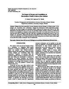
In order to illustrate the non-parametric method, we produce and evaluate non-parametric estimates of the one-step ahead prediction distributions for realized volatility on the S&P500 market index, …tting the model described in (37) and (38). The sample period extends from 2 January 1998 to 29 August 2008, providing a total of 2645 daily observations. All index data has been supplied by the Securities Industries Research Centre of Asia Paci…c (SIRCA) on behalf of Reuters, with the raw index data having been cleaned using the methods of Brownlees and Gallo (2006).12 The time series of the data is plotted in Panel A of Figure 1. As is clear from that …gure, there are several distinct periods in which volatility is seen to be signi…cantly higher than during the remaining sample period. The …rst of these periods corresponds to the Asian currency crisis in 1998, whereby a …nancial crisis gripped much of Asia and raised fears of a worldwide economic slowdown. Realized volatility also reached high levels at the end of year 2000, following the burst of the ‘Dot-com’bubble, and in year 2001 after the September 11th terrorist attacks in the United States. Year 2002 produced record values of realized volatility caused by a sharp 12 The authors would like to acknowledge the excellent research assistance of Chris Tse in producing the realized variance series. The realized variation measure is based on …xed …ve minute sampling, with a ‘nearest price’method used to construct arti…cial returns …ve minutes apart. Subsampling (or averaging) over the day is also used, in order to mitigate some of the e¤ects of microstructure noise. See Martin et al. (2009) for details of such computations.

25

drop in stock prices, generally viewed as a market correction to over-in‡ated prices following a decade-long ‘bull’market. Also factoring in the speed of the fall in prices at this time were a series of large corporate collapses (e.g. Enron and WorldCom), prompting many corporations to revise earnings statements, and causing a general loss of investor con…dence. The …nal period of high volatility in our sample corresponds to the year 2008, associated with the ‘global …nancial crisis’, triggered by the sub-prime mortgage defaults in the United States. During all of these periods, the peaks reached by the realized volatility values were between ten and twenty times larger than the average level over the full sample period. In contrast, there was a relatively long period of time, from 2003 to mid-2007, during which volatility was relatively stable and low. Panel B of Figure 1 plots the histogram of log realized volatility, with the distinct skewness to the right re‡ecting the occurrence of the very extreme values of realized volatility itself.13 These empirical characteristics are consistent with the existence of a jump di¤usion model for the stock prices index, with realized volatility re‡ecting both di¤usive and jump variation as a consequence. In using the non-parametric approach to estimate the forecast distribution for log realized volatility the aim is to capture the impact of the jump variation in a computational simple way, rather than modelling price jumps explicitly.

4.2

Empirical results

We divide the S&P500 daily realized volatility data into two subsamples. The …rst subsample (2 January 1998 to 30 January 2007), containing 2245 observations, is reserved for estimation of the model parameters in (37) and (38), including the unknown ordinates of p( ): The subsample used for forecast assessment comprises the remaining 400 realized volatility values, covering the period from 31 January 2007 to 29 August 2008, and as represented by the shaded area in Panel A of Figure 1. This subsample period corresponds to the early period of the …nancial crisis, during which defaults on sub-prime mortgages began to impact on the viability of …nancial institutions and the availability of credit. The out-of-sample density forecasts are based on (parameter) estimates updated as the estimation window expands with each new daily observation. N = 21 grid points, equally spaced over the interval from -10 to 10, are used to represent the support of the measurement error density, p ( ). Values of the penalty parameters used in (24) are

= 4; c = 0:5 and ! = 0:3.14

We estimate the 400 one-step ahead predictive distributions for the level of realized volatility for the out-of-sample period. For each of the 400 prediction distributions, simulated draws 13

A Jarque-Bera test applied to this log realized volatility series rejects the null hypothesis of Gaussianity at any conventional level of signi…cance. 14 Robustness of the results to di¤erent values of N (in a range from 21 to 51) for a …xed set of penalty values, and robustness of the results to di¤erent sets of penalty values (1 4; 0:01 c 0:5; 0:3 ! 0:8 ) was investigated. Di¤erences in the estimated forecast distributions were negligible.

26

Panel A: Time series of realized volatility .28 .24 .20 .16 .12 .08 .04 .00 1998

1999

2000

2001

2002

2003

2004

2005

2006

2007

2008

Panel B: Histogram of log realized volatility 320 280

Frequency

240 200 160 120 80 40 0 -8.0

-7.5

-7.0

-6.5

-6.0

-5.5

-5.0

-4.5

-4.0

-3.5

-3.0

-2.5

-2.0

-1.5

-1.0

Figure 1: Time series of realized volatility and histogram of log realized volatility of S&P500 market index from 2 January 1998 to 29 August 2008.

27

.14 .12 .10 .08 .06 .04 .02

1 Aug 08

1 Jul 08

2 Jun 08

1 May 08

1 Apr 08

3 Mar 08

1 Feb 08

1 Jan 08

3 Dec 07

1 Nov 07

1 Oct 07

3 Sep 07

1 Aug 07

2 Jul 07

1 Jun 07

1 May 07

2 Apr 07

1 Mar 07

1 Feb 07

.00

Low er bound Realised Volatility Upper bound

Figure 2: 95% one-step-ahead prediction intervals and the observed realized volatility, over the 400 day evaluation period (31 January 2007 to 29 August 2008)

of ln RVT +1 (in terms of which the measurement equation is speci…ed) are exponentiated to produce future values of RVT +1 ; with these values then used to produce a sequence of 95% prediction intervals for the evaluation period in Figure 2. The solid line represents the observed RVt at each point t in the evaluation period, while the dotted lines represent the 2.5% and 97.5% predictive bounds. The empirical coverage for the evaluation period is 94.0%, insigni…cantly di¤erent from the nominal level of 95% and providing, thereby, extremely strong support for the overall accuracy of the non-parametric approach. Support is also provided via the Pearson test for uniformity of the probability integral transform series, u in (43). However, both the LR test of the normality (and independence) of ! iT +1 ; i = 1; 2; :::; M in (44) and the Jarque-Bera test for the normality of ! iT +1 ; i = 1; 2; :::; M in (44) lead to rejection, indicating that some aspect of the forecast distribution is not being adequately captured. Observation of the shape of the histogram of u in Figure 3, indicates that too many realizations of volatility fall in the right tail of the forecast density, relative to the estimate thereof. This suggests that, despite the overall predictive accuracy evidenced, we are still unable to capture the most extreme values of volatility that occur on a few occasions during the evaluation period. 28

.10 .09

Relative Frequency

.08 .07 .06 .05 .04 .03 .02 0.0

0.1

0.2

0.3

0.4

0.5

0.6

0.7

0.8

0.9

1.0

Figure 3: Histogram of the probability integral transform series, u, for the realized volatility model. The horizontal lines superimposed on the histogram are approximate 95% con…dence intervals for the individual bin heights under the null that u is i:i:d: U (0; 1) :

4.3

Measuring sampling error

Finally, in the context of producing estimates of forecast distribution that are conditional on estimates of the …xed parameters, it is of interest to consider the issue of sampling error and the appropriate measurement thereof. In the spirit of McCabe et al. (2011) the subsampling approach of Politis, Romano and Wolf (1999) is used to quantify sampling variation in a single estimated one-step-ahead forecast distribution, for 17th March 2008, a quite high volatility day during the out-of-sample period. The technique mimicks the conventional prediction interval for a scalar point forecast, but ensures, at the same time, that the integration to unity property of the forecast distribution still holds.15 The steps of the procedure are as follows: 1. Obtain T b+1 subsamples Y1 = (y1 ; : : : ; yb ) ; Y2 = (y2 ; :::; yb+1 ); :::; YT

b+1

= (yT

b+1 ; :::; yT )

0

from the set of empirical data, y1:T = (y1 ; y2 ; :::; yT ) : 2. Use the proposed non-parametric ML method to produce an estimate of , ^b;t , computed 15

In related work, Rodriguez and Ruiz (2009) present a bootstrap-based approach to estimating prediction intervals in a linear state space setting. Their method uses the Kalman …lter recursions, but eschews the assumption of Gaussian innovations by using random draws from the empirical distributions of the innovations. It also factors sampling variation into the prediction intervals, but in a di¤erent way from that proposed by McCabe et al. (2011) and followed in this paper. See also Pascual, Romo and Ruiz (2001, 2005).

29

from Yt , for t = 1; 2; :::; T

b + 1:

3. Use ^b;t and the observed values, y1:T , to compute the 1-step ahead forecast distribution p yT +1 jy1:T ; ^b;t : 4. Calculate (over an arbitrarily …ne grid of values for yT +1 ) the metric p db;t = T p yT +1 jy1:T ; ^b;t p yT +1 jy1:T ; ^ , where p yT +1 jy1:T ; ^ is the estimated 1 forecast distribution based on the empirical data and ^ is the empirical estimate of : 5. Find the 95th percentile of fdb;1 ; : : : ; db;T

b+1 g,

d0:95 b ; and the corresponding distribution

p0:95 (yT +1 jy1:T ; ) : Then, relative to the replicated distributions and in terms of the jj:jj1 distance from p yT +1 jy1:T ; ^ , the chances of seeing a distribution as or more ‘extreme’

than p0:95 (yT +1 jy1:T ; ) is 5%.

The data-dependent method used to choose the size of the sub-samples, b (see Politis et al., 1999, Chapter 9) is as follows: a. For each b 2 fbsmall ; : : : ; bbig g carry out Steps 1 to 5 above to compute db0:95 . b. For each b compute V Ib as the standard deviation of the 2k + 1 consecutive values 0:95 d0:95 b k ; : : : ; db+k (for k = 2).

c. Choose ^b to minimise V Ib .16 Figure 4 shows the 10th, 50th and 95th percentile sub-sampled forecasts, along with the estimated empirical forecast, for the 17th March 2008. Panel A shows the relevant results based on a sample size of 505 observations (approximately two trading years) with ^b = 255. Panel B shows the results based on 2528 observations, with ^b = 1300. As is clear, for the smaller sample size, there is a large amount of uncertainty in the predictive estimate, with that uncertainty serving to shift probability mass across the support of the predictive distribution. For example, the predictive distribution at the 50th percentile assigns a larger probability to extreme values of volatility, than does the actual empirical estimate. On the other hand, the predictive distribution at the 95th percentile assigns large probabilities to very low values of volatility. In other words, for the smaller sample size sampling variability has a substantial impact, serving to alter the qualitative nature of conclusions drawn about future volatility. For the larger sample size, the subsampled-based sampling distribution of the (estimated) forecast 16

We have chosen to use d0:95 as the percentile on which selection of b is based as we are interested, primarily, b in ascertaining the changes in the forecast distributions that may occur at the extreme end of the scale (of the metric d).

30

PANEL A

PANEL B

120

40 35

100

30 80 25 60

20 15

40

10 20 5 0

0 .00

.01

.02

.03

.04

.05

.06

.07

.08

.09

.10

.11

.12

.13

.00

RV

.01

.02

.03

.04

.05

.06

.07

.08

.09

.10

.11

.12

.13

RV

Empirical Forecast 10th Percentile 50th Percentile 95th Percentile

Figure 4: Plot of the 10th, 50th and 95th percentile bootstrap forecast against the empirical forecast for the 17th March 2008. Panel A shows the bootstrap forecasts estimated from the preceding 505 observations. Panel B shows the bootstrap forecasts estimated from the preceding 2528 observations.

distribution becomes much more concentrated around the empirical estimate, with the full suites of distributions leading to qualitatively similar conclusions regarding volatility on the given day.

31

5

Concluding Remarks

We have developed a new method for estimating the full forecast distribution of non-Gaussian time series variables in the context of a general non-Gaussian, non-linear state space model. A non-parametric …lter is derived that exploits the functional relationship between the observed variable and the state and measurement error variables, expressed using Dirac’s -function. This representation, along with a simple rectangular integration rule de…ned over the …xed support of the measurement error, allows the density of the measurement error to be estimated at N grid points using a penalized likelihood procedure. The approach enables predictive distributions to be produced with computational ease in any model in which the relationship between the measure and state is well understood, but the precise distributional form of the measurement error is unknown. The method is developed in the context of a model for a scalar measurement and state, as is suitable for many empirical problems, with extension to higher dimensional problems also feasible, subject to the usual proviso that accompanies a grid-based method. Using the proposed method, the predictive distributions for the observed and latent variables are produced for a range of linear and non-linear models, in a simulation setting. The non-parametric predictive distributions are compared against distributions produced via (misspeci…ed) parametric approaches. Results show that the non-parametric method performs signi…cantly better, overall, than (misspeci…ed) parametric alternatives and is competitive with correctly speci…ed parametric estimates. The new method is also applied to empirical data on the S&P500 index, with the non-parametric predictive distribution able to capture important distributional information about the future value of the realized volatility of the index. A subsampling method is used to highlight the e¤ect that sampling variation can have on predictive conclusions, in small samples in particular. We conclude by noting that despite our focus here on the non-parametric setting, our proposed algorithm is also directly applicable to models in which the measurement error distribution is speci…ed parametrically. In that particular case, as long as the measurement error distribution is able to be simulated from and an appropriate transformation between each measurement and its error term is available, then the grid-based method may be replaced by an approach in which all relevant integrals are evaluated by Monte Carlo simulation, based on draws from the invariant distribution of the measurement error. The resulting alternative particle …lter, unnecessary in scalar (or low) dimensional cases such as those explored in this paper, would be a powerful tool in high-dimensional settings, particularly as it avoids the degeneracy problems that are a feature of existing simulation-based …ltering algorithms. This is currently the subject of investigation by the authors.

32

References [1] Ait-Sahalia, Y. and Lo, A.W. 1998. Nonparametric Estimation of State-Price Densities Implicit in Financial Asset Prices. Journal of Finance 53, 499-547. [2] Amisano, G. and Giacomini, R. 2007. Comparing Density Forecasts via Weighted Likelihood Ratio Tests. Journal of Business and Economic Statistics 25, 177-190. [3] Anderson, B.D.O. and Moore, J.B. 1979. Optimal Filtering. Prentice. [4] Andersens, T.G., Bollerslev,T., Diebold, F.X. and Ebens, H. 2001. The Distribution of Realized Stock Return Volatility. Journal of Financial Econometrics 61, 43-76. [5] Andersens, T.G., Bollerslev, T., Diebold, F.X. and Labys, P. 2003. Modeling and Forecasting Realized Volatility. Econometrica 71, 579-625. [6] Arulampalam, M. S., Maskell, S., Gordon N. and Clapp, T. 2002. A Tutorial on Particle Filters for Online Nonlinear/Non-Gaussian Bayesian Tracking. IEEE Transactions on Signal Processing 50 (2), 174-188. [7] Au, C. and Tam, J. 1999. Transforming Variables Using the Dirac Generalized Function. The American Statistician 53, 270-272. [8] Barndor¤-Nielsen, O.E. and Shephard, N. 2002. Econometric Analysis of Realized Volatility and Its Use in Estimating Stochastic Volatility Models. Journal of the Royal Statistical Society. Series B (Statistical Methodology) 64, 253-280. [9] Bates, D. 2000. Post-87 Crash Fears in the S&P 500 Futures Option Market. Journal of Econometrics 94, 181-238. [10] Bauwens, L. and Veredas, D. 2004. The Stochastic Conditional Duration Model: A Latent Variable Model for the Analysis of Financial Durations. Journal of Econometrics 199, 381-412. [11] Bauwens, L, Giot, P, Grammig, J and Veredas, D. 2004. A Comparison of Financial Duration Models via Density Forecasts. International Journal of Forecasting 20, 589-609. [12] Berg, J.E., Geweke, J. and Rietz, T.A. 2010. Memoirs of an Indi¤erent Trader: Estimating Forecast Distributions from Prediction Markets, Quantitative Economics 1, 163-186. [13] Berkowitz, J. 2001. Testing Density Forecasts with Applications to Risk Management, Journal of Business and Economic Statistics 19, 465–474. 33

[14] Boero, G., Smith, J. and Wallis, K.F. 2011. Scoring Rules and Survey Density Forecasts. International Journal of Forecasting 27, 379-393. [15] Broadie, M., Chernov, M. and Johannes, M. 2007. Model Speci…cation and Risk Premia: Evidence from Futures Options. The Journal of Finance LXII: 1453 - 1490. [16] Brownless, C.T. and Gallo, G.M. 2006. Financial Econometrics Analysis at Ultra-High Frequency: Data Handling Concerns, Computational Statistics and Data Analysis 51, 22322245 [17] Bu, R. and McCabe, B.P.M. 2008. Model Selection, Estimation and Forecasting in INAR(p) Models: A Likelihood based Markov Chain Approach, International Journal of Forecasting 24, 151-162. [18] Caron, F, Davy, M, Doucet, A and Du‡os, E. 2008. Bayesian Inference for Linear Dynamic Models with Dirichlet Process Mixtures. IEEE Transactions on Signal Processing 56, 7184. [19] Clements, A., Hurn, S. and White, S. 2006. Estimating Stocahstic Volatility Models Using a Discrete Non-Linear Filter. Working Paper No. 3. National Centre for Econometric Research. [20] Czado, C., Gneiting, T. and Held, L. 2009. Predictive Model Assessment for Count Data. In press, Biometrics. [21] Dawid, A.P. 1984. Present Position and Potential Developments: some personal views: statistical theory: the prequential approach. Journal of the Royal Statistical Society, Series A 147, No. 2, 278-292. [22] De Rossi, G. and Harvey, A. 2009. Quantiles, expectiles and splines. Journal of Econometrics 152, 179-85. [23] Diebold, F.X., Gunther, T.A. and Tay, A.S. 1998. Evaluating Density Forecasts with Applications to Financial Risk Management. International Economic Review 39, 863-883. [24] Durham, G.B. 2007. Monte Carlo Methods for Estimating, Smoothing and Filtering Oneand Two-Factor Stochastic Volatility Models. Journal of Econometrics 133, 273-305. [25] Durham, G.B. 2007. SV Mixture Models with Application to S&P 500 Index Returns. Journal of Financial Econometrics 85, 822-856.

34

[26] Engle, R.F. and Gonzalez-Rivera, G. 1991. Semiparametric ARCH Models. Journal of Business and Economic Statistics 9, 345-359. [27] Eraker, B., Johannes, M.S. and Polson, N.G. 2003. The Impact of Jumps in Returns and Volatility, Journal of Finance 53, 1269–1300. [28] Fernandez, C. and Steel, M.F.J. 1998. On Bayesian Modelling of Fat Tails and Skewness, Journal of the American Statistical Association 93, 359-371 [29] Freeland, R and McCabe, B. 2004. Forecasting Discrete Valued Low Count Time Series. International Journal of Forecasting 20, 427-434. [30] Geweke, J. and Amisano, G. 2010. Comparing and Evaluating Bayesian Predictive Distributions of Asset Returns, International Journal of Forecasting (Special Issue on Applied Bayesian Forecasting in Economics) 26, 216-230. [31] Giacomini, R. and Komujer, I. 2005. Evaluation and Combination of Conditional Quantile Forecasts. JBES 23, 416-431. [32] Gneiting, T. 2008. Editorial: Probabilistic Forecasting, Journal of the Royal Statistical Society (A) 171, 319-321. [33] Gneiting, T. and Raftery, A.E. 2007. Strictly Proper Scoring Rules, Prediction, and Estimation, Journal of the American Statistical Association 102, 359-378. [34] Gneiting, T., Balabdaoui, F. and Raftery, A.E. 2007. Probabilistic Forecasts, Calibration and Sharpness. Journal of Royal Statistical Society 69, 243-268. [35] Hassani, S. 2009. Mathematical Methods for Students of Physics and Related Fields (2nd Edition). [36] Jensen, M.J. and Maheu, J.M. 2010. Bayesian Semiparametric Stochastic Volatility Modeling. Journal of Econometrics 157, 306-316. [37] Johnson, N.L., Kotz, S. and Balakrishnan, N. 1994. Distributions in Statistics: Continuous Univariate Distributions, Vol. 2. Wiley, New York [38] Kitagawa, G. 1987. Non-Gaussian State Space Modeling of Nonstationary Time Series. Journal of the American Statistical Association 76, 1032-1064. [39] Kitagawa, G. 1994. The Two-Filter Formula for Smoothing and an Implementation of the Gaussian-sum Smoother. Annals of the Institute of Statistical Mathematics 46, 605-623. 35

[40] Khuri, A.I. 2004. Application of Dirac’s Delta Function in Statistics. International Journal of Mathematical Eduction in Science and Technology 35, 185-195. [41] Lim, G, Martin, G and Martin, V, 2005. Parametric Pricing of Higher Order Moments in S&P500 Options. Journal of Applied Econometrics 20, 377-404. [42] McCabe, B and Martin, G. 2005. Bayesian Predictions of Low Count Time Series. International Journal of Forecasting 21, 315-330. [43] McCabe, B., Martin, G.M. and Harris, D. 2011. E¢ cient Probabilistic Forecasts for Counts. Forthcoming, Journal of the Royal Statistical Society, Series B 73, 253-272. [44] Martin, G, Reidy, A and Wright, J. 2009. Does the Option Market Produce Superior Forecasts of Noise-corrected Volatility Measures. Journal of Applied Econometrics 24, 77104. [45] Monteiro, A.A. 2010. A Semiparametric State Space Model. Working paper, Statistics and Econometrics Series Universidad Carlos III de Madrid, Spain. Available at http://earchivo.uc3m.es/bitstream/10016/9247/1/ws103418.pdf. [46] Pascual, L., Romo, J. and Ruiz, E. 2001. E¤ects of parameter estimation on prediction densities: a bootstrap approach. International Journal of Forecasting 17, 83-103. [47] Pascual, L., Romo, J. and Ruiz, E. 2005. Bootstrap prediction intervals for powertransformed time series. International Journal of Forecasting 21, 219-235. [48] Politis, D.N., Romano, J.P. and Wolf, M. 1999. Subsampling, Springer, New York. [49] Rodriguez, A. and Ruiz, E. 2009. Bootstrap Prediction Intervals in State-Space Models. Journal of Time Series Analysis 30, 167-178. [50] Rosenblatt, R.F. 1952. Remarks on a Multivariate Transformation. Annals of Mathematical Statistics 23, 470-472. [51] Scott, D.W., Tapia, R.A. and Thompson, J.R. 1980. Nonparametric Probability Density Estimation by Discrete Maximum Penalized-Likelihood Criteria. Annals of Statistics 8, 820-832. [52] Sorenson H.W. and Alspach D.L. 1971. Recursive Bayesian Estimation Using Gaussian Sums. Autmatica 7, 465-479

36

[53] Strickland, C.M., Forbes, C.S. and Martin, G.M. 2006. Bayesian Analysis of the Stochastic Conditional Duration Model. Computational Statistics and Data Analysis (Special Issue on Statistical Signal Extraction and Filtering) 50, 2247-2267. [54] Tay, A and Wallis, K. 2000. Density forecasting: A Survey. Journal of Forecasting 19, 235-254. [55] Yau, C., Papaspiliopoulos, O., Roberts, G.O. and Holmes, C. 2011. Bayesian nonparametric hidden Markov models with applications in genomics. Journal of the Royal Statistical Society, Series B 73, 37-57.

37