Non-parametric kernel estimation for symmetric Hawkes processes ...

EPJ manuscript No. (will be inserted by the editor)

Non-parametric kernel estimation for symmetric Hawkes processes. Application to high frequency financial data. Emmanuel Bacry1 , Khalil Dayri1 , and Jean-Francois Muzy1,2 1

arXiv:1112.1838v1 [q-fin.TR] 8 Dec 2011

2

a b

.

CMAP UMR 7641 CNRS, Ecole Polytechnique, 91128 Palaiseau, France SPE UMR 6134 CNRS, Universit´e de Corse, 20250 Corte, France December 9, 2011 Abstract. We define a numerical method that provides a non-parametric estimation of the kernel shape in symmetric multivariate Hawkes processes. This method relies on second order statistical properties of Hawkes processes that relate the covariance matrix of the process to the kernel matrix. The square root of the correlation function is computed using a minimal phase recovering method. We illustrate our method on some examples and provide an empirical study of the estimation errors. Within this framework, we analyze high frequency financial price data modeled as 1D or 2D Hawkes processes. We find slowly decaying (power-law) kernel shapes suggesting a long memory nature of self-excitation phenomena at the microstructure level of price dynamics. PACS. 02.50.Ey Stochastic processes – 05.45.Tp Time series analysis – 02.70.Rr General statistical methods – 89.65.Gh Economics; econophysics, financial markets, business and management

1 Introduction Although the concept of self excitement was commonly used for a long time by seismologists (see [30] and the references therein), Alan Hawkes was the first to provide a well defined point process with a self exciting behavior [13, 14,19]. This model was introduced to reproduce the ripple effects generated after the occurrence of an earthquake [31,1]. Since then, it has been successfully used in many areas ranging from seismology (see e.g., [23], for a recent review), biology [28], to even criminology and terrorism [21,10] (cf [19] and references therein for a detailed review of Hawkes processes and their applications). As far as financial applications are concerned, since transactions and price changes are discrete events, Hawkes processes have naturally been generating more and more interest. Applications can be found in the field of order arrival rate modeling [16,7,29], noise microstructure dynamics [2], volatility clustering [11], extreme values and VaR estimation [8] and credit modeling [12]. Hawkes models account for a self exciting behavior of events by which the arrival of one event increases the probability of occurrence of new ones. In its most basic form and in the one dimensional case, the Hawkes process is a counting process defined by λt , the rate of arrival of events a

This research is part of the Chair Financial Risks of the Risk Foundation. b The financial data used in this paper have been provided by the company QuantHouse EUROPE/ASIA, http://www.quanthouse.com

by: λt = µ +

Z

t

φt−s dNs

(1)

−∞

where µ > 0 is a constant background rate, Nt is the cumulative counting process and φ a positive real function called decay kernel. We can clearly see in equation (1) that when some event occurs at time t, we have dNt = 1 and hence dλt = φ0 . The influence of the event is transmitted to future times through φ such that at time u > t the increase in λt due to the time t event is φu−t . Thus a self exciting behavior is observed. A basic issue in applications of Hawkes processes concerns their estimation. In early applications, parametric estimation used spectral analysis by means of the Bartlett spectrum (the Fourier transform of the autocovariance of the process) [4,5] and it was indeed through that light that Hawkes presented his model. A maximum likelihood method for estimating the parameters of exponential, power law and Laguerre class of decay kernels was developed in [26,24] and it became the standard method for estimating Hawkes processes. Furthermore, the Laguerre decay kernels were seen to be very pertinent decay kernels because they allowed to account for long term dependencies as well as offering short term flexibility. More recently, other types of estimation procedures were developed. When the form of the decay kernel is unknown, non-parametric methods are desirable because they give an idea of their general shape. For example, by using the branching property of the Hawkes process [32], the authors in [20] and [18] were able to provide Expectation-Maximization algorithms to

2

Emmanuel Bacry et al.: Non-parametric Hawkes kernel estimation

R estimate both background rate and the decay kernel. In – For any function ft , fbz = R e−zt ft dt corresponds to [28], the authors present also an algorithmic method for its Laplace transform. cz ∈ Mn,p (C) decay estimation by using a penalized projection method. – By extension if Mt ∈ Mn,p (R) then M In this paper, we propose an alternative simple non corresponds to the matrix whose elements are the Laplace parametric estimation method for multivariate symmettransforms of the elements of Mt . ric Hawkes processes based on the Bartlett spectrum. We Using these notations, one of the main results of Hawkes present the method and its numerical feasibility without going too much in details about convergence speeds or is that if error optimization. By studying one dimensional and 2ij dimensional examples, we show that our approach pro- H1 the kernel φt ∈ Mn,n is positive (φt ≥ 0, ∀t) and causal (φt = 0, ∀t < 0), vides reliable estimates on both fast and slowly decaying and kernels. We then apply our method to high frequency financial data and find power-law kernels. This implies that H2 the spectral radius of φb0 (i.e., its largest eigen value) is strictly smaller than 1, the arrival of events display long range correlations, a phenomenon well known in finance, similarly to what was sugthen (Nt )t≥0 is a n-dimensional point process with stagested in [6]. tionary increments. The conditional intensity λt is itself a This paper is organized as follows. In section 2, we instationary process with mean troduce a basic version of a multivariate Hawkes processes. We place ourselves in the context of an n−dimentional linΛ = E(λt ) = E(dNt )/dt. (3) ear Hawkes process with a constant background rate and a nonnegative decay kernel. We set some notations and give Combining this last equation with Eq. (2), one easily gets R∞ Rt out a martingale representation of the rate function λt in Eq. (1). In section 3, we study the autocovariance of the Λ = µ + −∞ φt−s dsΛ = µ + 0 φu duΛ and consequently process. Along the same line as [14], we establish its relaΛ = (I − φb0 )−1 µ, (4) tionship with the decay kernel in both direct and Fourier spaces. The estimation method in the case of symmetric Hawkes processes is then provided in section 4. This where I refers to the n × n identity matrix. Before moving on, we need to introduce some more method, based on a Hilbert transform phase recuperation method, is explicitly detailed in both univariate and spe- notations that will be used all along the paper. cial symmetric bivariate cases. In section 5, the method is illustrated by numerical examples for both exponential Notations 2 If At ∈ Mm,n (R) and Bt ∈ Mn,p (R) then R Bt is naturally defined R product of At and and power law kernels. We also address some statistical is- the convolution A B ds. Of course it A B ds = as A ⋆ B = s t−s t R t−s s R sues concerning the estimation errors. Finally, in section 6, is associative and distributive however it is generally not we apply our method to high frequency financial data for commutative (unless A and B are commutative). The t t which we deduce a long range nature of the decay kernels. neutral element is δIt , i.e., the diagonal matrix with Dirac distribution on the diagonal. In the following we will use the notation : 2 Multivariate Hawkes Processes Z At−s dNs . A ⋆ dNt = 2.1 Notations and Definitions R

As introduced by Hawkes in [13] and [14], let us consider an n-dimensional point process (Nt )t≥0 , where Nti 1 ≤ i ≤ n represents the cumulative number of events in the ith component of the process Nt up to time t. The conditional intensity vector at any time t is assumed to be a random process that depends on the past as Z t λt = µ + φt−s dNs (2)

Combining both Notations 1 and 2, it is easy to show that the convolution theorem on matrices translates in bz . bz B \ A ⋆ Bz = A 2.2 Martingale representation of λt

where µ is a vector of size n with strictly positive components (µi > 0) and φt is an n × n matrix referred to as the decay kernel.

We roughly follow a similar path to Hawkes in [14]. Let (Mt )t≥0 be the martingale compensated process of (Nt )t≥0 defined by: dMt = dNt − λt dt . (5)

Notations 1 In the following

Then λt can be represented as a stochastic integral with respect to the martingale (Mt )t≥0 :

−∞

– Mn,p (R) (resp. Mn,p (C)) denotes the set of n × p matrices with values in R (resp. C). For any matrix M (resp. vector v), M ij (resp. v i ) denotes its elements.

Proposition 1 One has: λt = Λ + Ψ ⋆ dMt ,

(6)


where Ψt is defined as Ψt =

3

Proof By using equation (5), we can write: ∞ X

(⋆n)

φt

,

(7)

E(dNt dNt†′ ) = E((dMt + λt dt)(dMt′ + λt′ dt′ )† ) = E(dMt dMt†′ )

n=1

+E(λt dMt†′ )dt +E(dMt λ†t′ )dt′ +E(λt λ†t′ )dtdt′

(⋆n)

where φt refers to the nth auto-convolution of φt (i.e., (⋆n) = (φ bz )n ) φ[ z Proof Using equations (2) and (5) one has:

λt = µ + φ ⋆ dNt = µ + φ ⋆ dMt + φ ⋆ λt , and consequently

Since µ is a constant one has h ⋆ µ = µb h0 . Using the convolution theorem one gets µb h0 = (I − φb0 )−1 µ = Λ which proves the proposition.

3 The covariance matrix of Hawkes processes The kernel estimator we are going to build is based on the empirical auto-covariance of (Nt )t≥0 . This section is devoted to the covariance matrix of the n-dimensional Hawkes processes. However, we first discuss some useful results about their infinitesimal auto-covariance function. 3.1 The infinitesimal covariance Let us define the infinitesimal covariance matrix:

(10) (11) (12)

We begin by noticing that (thanks to martingale property), E(dMt dMt†′ ) = 0, ∀t 6= t′ . As for when t = t′ , we have for all 1 ≤ i < j ≤ n E(dMti dMtj ) = 0

(δI − φ) ⋆ λt = µ + φ ⋆ dMt . Let us note that the inverse of δIt − φt for the convolution product is nothing but ht = δIt + Ψt . Thus convoluting on each side of the last equation by ht , one gets (since h ⋆ φt = Ψt ) λt = h ⋆ µ + Ψ ⋆ dMt .

(9)

since the N i ’s (and hence the M i ’s) for 1 ≤ i ≤ n have no jump in common. Moreover, for i = j we have E(dMti dMti ) = Λi dt because E(dMti dMti ) = E(dNti dNti ) and E(dNti dNti ) = E(dNti ) = Λi dt since the jumps of Nt are of size 1. To sum up, the term (9) becomes: E(dMt dMt†′ ) = Σδt−t′ dtdt′

(13)

The remaining terms can be then calculated along the same line. Replacing λt ’s expression from equation (6) in the term (10), gives: E(λt dMt†′ )dt = E Ψ ⋆ dMt dMt†′ dt,

or in other words

E(λt dMt†′ )dt

=

Z

R

Ψt−s E(dMs dMt†′ )dtds

and thanks to equation (13), Z † Ψt−s Σδs−t′ dsdt′ dt E(λt dMt′ )dt = R

νt−t′ = E(dNt dNt†′ ), †

where M denotes the hermitian conjugate of a matrix M . Along the same way as Hawkes in [14], νt−t′ can be related to the decay kernel φ. We present in proposition 2 an equation linking the infinitesimal covariance matrix to Λ and Ψ but, unlike Hawkes, we express ν explicitly as a function of Ψ and Λ instead of an integral equation in ν. This result will be at the heart of the estimation method we propose in this paper. Proposition 2 Let (Nt )t≥0 be an n-dimensional Hawkes process with intensity λt as defined in Section 2.1 (assuming both H1 and H2). Let Ψet = Ψ−t . We have the following result: E(dNt dNt†′ ) = ΛΛ† + Σδt−t′ + Ψt−t′ Σ + ΣΨt†′ −t (8) + Ψe ⋆ ΣΨt†′ −t dtdt′ where Σ is the diagonal matrix defined by Σ ii = Λi for all 1 ≤ i ≤ n and δt is the Dirac distribution.

that is simplified to: E(λt dMt†′ )dt = Ψt−t′ Σdtdt′

(14)

Similarly, the term (11) becomes: E(dMt λ†t′ )dt′ = ΣΨt†′ −t dtdt′

(15)

and finally, using Eq. (13), the term (12) can be written as: E(λt λ†t′ )dtdt′ = ΛE(λ†t′ ) + E((Ψ ⋆ dMt )λ†t′ dtdt′ Z † † Ψt−s E(dMs λt′ ds) dtdt′ = ΛΛ + R Z † † = ΛΛ + Ψt−s ΣΨt′ −s ds) dtdt′ R

′

By setting u = t − s, we get: E(λt λ†t′ )dtdt′ = ΛΛ† + Ψe ⋆ ΣΨt†′ −t dtdt′ ,

which ends the proof of the proposition.

(16)

4


and conversely:

3.2 The covariance matrix The (normalized) covariance matrix of the Hawkes process can be defined, at scale h and lag τ , by vτ(h)

=h

−1

Cov (Nt+h − Nt , Nt+h+τ − Nt+τ ) ,

(17)

where we normalized by h in order to avoid a trivial scale dependence. Let us note that, since the increments of Nt are stationary, the previous definition does not depend on t. Thus, it can be rewritten as ! Z τ +h Z h 1 † † (h) dNs − Λ h) (18) dNs − Λh)( vτ = E ( h τ 0 It is clear that this quantity can be easily estimated on real data using empirical means. As we will see, the non parametric estimation of the decay kernel we propose in this paper is based on these empirical estimations. More precisely, it is based on the following Theorem. (h)

Theorem 1 Let gt = (1 − (h) as a function of gτ and Ψτ :

|t| + h) .

(h)

vτ

can be expressed

vτ(h) = gτ(h) Σ+g (h) ⋆Ψ−τ Σ+g (h) ⋆ΣΨτ† +g (h) ⋆Ψe ⋆ΣΨτ† (19)

Proof Let us begin the proof by noticing that for any function f with values in R+ we have: Z h Z τ +h (h) h−1 (20) ft−t′ dt′ dt = f ⋆ g−τ 0

τ

It follows that vτ(h) = −

cz φbz = (I + Ψbz )−1 Ψ

(22)

vbz(h) = b gz(h) (I + Ψbz∗ )Σ(I + Ψbz∗ )†

(23)

Theorem 3.2 gives way to the following corollary. Corollary 1 In Laplace domain equation (19) becomes:

4 Non-parametric estimation of the kernel φt 4.1 The estimation principle In this paper, we aim at building an estimator of φt based (h) on empirical measurements of vτ . Let us note that empir(h) ical measurements of vτ are naturally obtained replacing probabilistic mean by empirical mean in Eq. (18) (see [3] for proof of convergence of the empirical mean towards the probabilistic mean). Thus, in order to build an es(h) timator, we need to express φt as a function of vτ . In b the Laplace domain, since a given ψz corresponds to a unique φbz (through Eq. (22)), it translates in trying to (h) express ψbz as a function of vbz which exactly corresponds to inverting Eq. (23) (i.e., computing the square root of (I + Ψbz∗ )Σ(I + Ψbz∗ )† ). Indeed, knowing ψbz , one easily gets φbz (from Eq. (22)) and finally φt . Actually, let us note that, from a practical point of view, we don’t need to work in the full complex domain z ∈ C of the Laplace transform. Working with the Fourier transform restriction (i.e., z = iω with ω ∈ R) is enough to recover φt . (h)

1 E h Z h

Z

h

dNs

0

Z

dNs†

dNs Λ h − Λh

0

1 = E h

τ +h

τ

†

Z

τ +h

dNs†

† 2

+ ΛΛ h

τ

Z

0

h

Z

τ

τ +h

Dealing with cancelations of gbz . The first problem that seems to appear for inverting this formula (23) (i.e., ex(h) pressing ψbz as a function of vbz only for z = iω) is the (h) (h) scalar term b gz that may vanish. Indeed, since gt = (1− (h) |t| + giω = (4/ω 2 h) sin2 (ωh/2), h ) , its Fourier transform, b 2nπ cancels for all ω of the form h , n ∈ Z, n 6= 0. Actually, this is not a real problem as long as

dNt dNt†′

† 2

− ΛΛ h

!

!

.

(h)

Using equation (8), we can split dNt dNt†′ into four parts and write: Z Z 1 h τ +h (Σδt−t′ vτ(h) = h 0 τ + Ψt−t′ Σ + ΣΨt†′ −t + Ψe ⋆ ΣΨt†′ −t dtdt′

By applying equation (20) to each of the terms under the double integral we get equation (19) and achieve the proof.

It is more convenient to rewrite the result of theorem (⋆n) = φ bn , Eq. (7) trans3.2 in Laplace domain. Since φ[ z z lates into : Ψbz =

+∞ X

n=1

φbnz = φbz (I − φbz )−1

(21)

– τ in the empirical estimation of vτ is sampled using a sampling period ∆ greater than h/2 (h) – ∆ is small enough so that b viω can be considered to have a compact support (h)

Indeed, if this is the case, then the estimation of vbiω (practically obtained by taking the Discrete Fourier Transform (h) (DFT) of the sampled signal (vk∆ )k ) will be equal on (h) [−π/∆, π/∆] to the product of the DFT of gτ (which does not vanish since [−π/∆, π/∆] ⊂ [−π/h, π/h]) and the DFT of (δτ + Ψe)Σ ⋆ (δτ + Ψe )†τ . Consequently, as long as h is small enough (so that ∆ can be chosen greater than h and small enough), dividing on both hand sides Eq. (23) (h) by gbz is not, from a practical estimation point of view, a real problem. So, in the following we will write (I + Ψbz∗ )Σ(I + Ψbz∗ )† = vbz(h) /b gz(h) ,

(24)

(h)

without bothering with eventual cancelations of gbz .


Computing the square root of (I + Ψbz∗ )Σ(I + Ψbz∗ )† . In (h) the estimation process, once we have estimated vτ and (h) consequently (through DFT) vbz (for z = iω), using Eq (24), we can estimate (I + Ψbz∗ )Σ(I + Ψbz∗ )† . We need to go from there to the estimation of Ψbz (then using Eq. (22), we get φbz and then by inverse Fourier transform φt ). This problem requires therefore to take the square root of the left hand side of Eq. (24). In dimension n = 1, it means being able to go from |1 + Ψbz |2 to Ψbz . There is clearly a phase determination problem. We will see that, in dimension n = 1, this phase is uniquely determined by the hypothesis H1 and H2. However, in dimension n > 1, they are many possible solutions and determining the correct one is not necessarily possible in general. We need to make a strong additional hypothesis. 4.2 Further hypothesis on the kernel φt In the following, we suppose that ¯ with ∀ i, E(λi ) = λ ¯ ∈ R, and φbz can be diagH3 Σ = λI t onalized into a matrix D with some constant unitary matrix U (that does not depend on z): φbz = U † Dz U.

(25)

5

The proof is based on the following theorem: Theorem 2 (Paley-Wiener [27]) Let’s suppose that we observe the amplitude |fbiω | of the Fourier transform of a real filter ft . If Z log(|fbiω |) dω < ∞, (30) 2 R 1+ω then the filter gt defined by its Fourier transform b

b

giω = elog(|fiω |)−iH(log(|fiω |)) , b

(31)

is the only causal filter (i.e., supported by R+ ), which is a phase minimal filter1 and which satisfies |b giω | = |fbiω |.

Proof of the Lemma. of this thepIt is a simple application (kk) orem with |fbiω | = Ezkk = |1 − Diω |−1 . Indeed, let us (kk) first show that gbz = (1−Dz )−1 is a minimal phase filter, i.e., that both the poles and zeros are such that ℜ(z) < 0.

– Let z be a zero of (1 − Dzkk )−1 , then it is a pole of Dzkk and consequently of φbz . However, from H1 and R +∞ H2 one concludes that |φbz | ≤ 0 |e−zt |φt dt cannot be infinite, unless ℜ(z) < 0. – Let z be a pole of (1−Dzkk )−1 . It thus satisfies Dzkk = 1. Thus 1 is an eigenvalue of φb0 which is in contradiction with H2. Thus (1 − Dzkk )−1 has no pole.

Let us point out that, though always true in dimension n = 1, H3 is a strong hypothesis for dimension n ≥ 2. Clearly it is satisfied in the case all the components of the process are identically distributed, i.e. the process is invariant under arbitrary permutations. Other cases are very specific and consequently are not discussed in this paper.

Consequently gbz = (1 − Dzkk )−1 is a minimal phase filter. Moreover, since every coefficients of φt are positive and in (kk) L1 , the Fourier transforms Diω , for any k, are continuous functions of ω and goes to 0 at infinity. Along with the fact that (1 − Dzkk )−1 has no pole and has its zeros on the halfplane ℜ(z) < 0 we easily conclude that |fbiω | = |1−Dzkk |−1 satisfies (30). The theorem above can be applied and the Lemma follows.

4.3 The estimator

Main steps for kernel estimation. The different steps for the final kernel estimator, in the fully symmetric case, can be summarized as follows

Using Eq. (21) along with H3, one gets that I + Ψbz∗ is diagonalizable in the same basis U and that I + Ψbz∗ = U † (I − Dz∗ )−1 U,

(26)

¯ g (h) ), Ez = U vbz(h) U † /(λb z

(27)

and thus from (24), one gets

where Ez is the diagonal matrix with the real positive coefficients : Ezkk = |1 − Dzkk |−2 . (28)

– Set ∆ small enough (see Section 4.1) and fix h = ∆, ¯ – Estimate the unconditional intensity λ, (h) – Estimate the auto-covariance operator vt and com(h) pute its Fourier transform vbiω , ∗ † ∗ ) using Eq. (24). Diagonalize – Compute (I+ Ψbiω )(I+ Ψbiω it and compute the matrix Eiω defined by Eq. (27), – Compute the diagonal matrix Diω using (29), – Go back to the initial basis and Inverse Fourier transform to get the estimation of φt .

So the estimation problem reduces to being able to recover the coefficients Dzkk from the coefficients Ezkk = |1 − Dzkk |−2 . This problem is solved by the following Lemma.

4.4 Some particular cases

Lemma 1 Let k be fixed. Let z = iω (with ω ∈ R). Then

4.4.1 The one dimensional case n = 1

(kk)

1

kk

1

kk

(1 − Diω )−1 = e 2 log |Eiω |−iH( 2 log |Eiω |) ,

(29)

where the operator H(.) refers to the Hilbert transform [25].

As we already pointed out, the hypothesis H3 is always true in this case since all the functions are scalar functions. 1

a minimal phase filter [25] is a filter whose all the zeros and the poles of its Laplace transform satisfy ℜ(z) < 0

6


Thus, the phase determination problem is solved without adding any assumption apart from H1 and H2. The kernel estimator simply consists in first computing (h)

vb |1 + Ψbiω |2 = iω(h) , ¯g λb iω

(32)

and then inverse Fourier transform of

b b φbiω = 1 − e− log |1+Ψiω |+iH(log |1+Ψiω |) .

(33)

5.1 The case n = 1

4.4.2 The bisymmetric 2-dimensional case n = 2

In the two-dimensional case, the hypothesis H3 is satisfied in the particular case µ1 = µ2 ,

(34)

and the kernel φt is bisymmetric, i.e., has the form 11 12 φt φt φt = 11 φ12 t φt

(h)11

¯ g (h) λb iω

(h)11

viω b

(h)12

+ vbiω

(h)12

− vbiω

¯ g (h) λb iω

= |1 +

11 Ψbiω

+

12 2 Ψbiω |

11 12 2 = |1 + Ψbiω − Ψbiω |

5.1.1 Exponential kernel We first simulate a one dimensional Hawkes process with an exponential kernel: φt = αe−βt 1t≥0

(35)

The matrix of the Laplace transform φbz can be indeed decomposed as follows: −φb11 + φb12 0 † z z b φz = U b12 U 0 φb11 z + φz −1 1 1 √ . where U = 2 1 1 Diagonalizing and identifying the diagonal coefficients in both hand sides of (27) leads to vbiω

(h)

We estimate vτ from the realization of a Hawkes process (Xt ), t ≥ 0 (1D or 2D). We then strictly follow the method described in previous section in order to estimate (h) the decay kernel φ. vτ is sampled at rate ∆ (i.e., τ = n∆) up to a maximum lag τmax . As explained in Section 4.1, in order to avoid problems related to the zeros of b g (h) , we naturally choose h = ∆. From a practical point of view, ∆ has to be chosen small enough in order to avoid Fourier aliasing.

(36) (37)

Applying the same method used in the case n = 1 to these last two equations, we get an estimate of Ψb . Finally we apply φbz = (I + Ψbz )−1 Ψbz (38)

b Applying the inverse transform to φb we finally giving φ. get φ. In the following section we illustrate these results and our methods on numerical simulations of 1D and 2D Hawkes processes.

5 Numerical illustrations Let us discuss some examples illustrating the estimation method as defined previously using simulated Hawkes processes. All the simulations have been performed with the thinning algorithm described in [22].

(39)

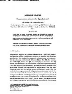
where we choose (µ = 1, α = 1, β = 4). This gives ¯ = 4/3. The simulated sample contains 130000 φb0 = 1/4, λ jumps (it is approximately T ≃ 105 seconds long). In figure 1(a) we have reported the estimated kernel function φt (circles) on top of the true kernel (solid line). We see that the estimated kernel function is, up to some noise, very close to the real kernel 5.1.2 Power Law Decay We now consider a power-law decaying kernel defined as: φt = α(t + γ)β 1t≥0

(40)

α γ β+1 . We with β < −1. In this case we have φb0 = − β+1 choose α = 32 and β = −5 and γ = 2 making φb0 = 0.5 < 1 ¯ = 2 again with 130000 jumps (T ≃ 65000 secs). The and λ kernel estimated on a single sample is reported in 1(b). Once again, one can see that, up to an additive noise, the estimated kernel fits well the real one. Let us point out that, since the decay is much slower than in the previous exponential case, we chose the maximum lag τmax to be ten times as much.

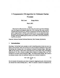
5.1.3 Error Analysis Let us briefly discuss some issues related to the errors associated with our kernel estimates. In ref. [3], a central limit theorem has been proved that shows that, asymptotically, the errors of the empirical covariance function estimates are normally distributed with a variance that decreases as T −1 (or N −1 for ∆ fixed). One thus expects the same kind of results in the estimates of the components of φ. Let us define the L2 estimation error as: τmax ∆

2

e =

X

k=1

(e)

|φk∆ − φk∆ |2

(41)


7

(a)

1

(a)

0.8 0

10

φ

e2

0.6 0.4 0.2 0 0

0.5

1

1.5

4

2

5

10

10

t

T 4

(b)

1

3

0.8

2

t=0.04 t=0.8 t=1.6

1

φ

Quantiles

0.6 0.4

0 −1 −2

0.2

−3 −4

0 0

2

4

6

8

10

t

Fig. 1. Non parametric estimation of a one dimensional Hawkes process using method described in Section 4.4.1 from a unique realization with 130000 jumps. Estimated (◦) and analytical kernel (solid line) are shown. (a) Case of the exponential decay kernel φ (Eq. (39)) with α = 1, β = 4. We used ∆ = 0.01 and τmax = 2. (b) Case of the power-law decay kernel φ (Eq. ((40))), with α = 32, β = −5 and γ = 2. We used ∆ = 0.05 and τmax = 20.

where φ(e) is the estimated kernel. In Fig. 2(a), we have reported e2 as a function of the sample length T for the same realization as the one used in Fig. 1(a). As expected, one observes a behavior very close to T −1 . Let us now look at the error between the analytical φ and the estimated one for a fixed t > 0. We find that, for each t, the series of errors are centered gaussian and mainly uncorrelated. Their variance increases as t decreases to 0. The normality of the observed errors is illustrated in Fig. 2(b) where we report, for 3 different values of t, the qq-plots of the empirical error pdf (with standardized variance) versus the normal pdf. Let us point out that the estimation error depends, a priori, on the sampling rate ∆. Numerical simulations show that there is an optimal choice for the sampling rate parameter ∆. Indeed, we found that the estimation error

−5 −4

(b) −2 0 2 Standard Gaussian Quantiles

4

Fig. 2. Error analysis of a one dimensional Hawkes process with the same exponential kernel as in Fig. 1(a) with ∆ = 0.01 and τmax=2 . (a) Mean square error as a function of the sample length T in log-log coordinates. The solid-line corresponds to the curve the expected T −1 behavior. (b) qq-plots of the Normal probability distribution function (pdf) versus empirical error pdf for φt for three different values of t. Here T = 105 seconds is fixed. The empirical error pdf’s have been normalized to have the same variance (the variance increases as t goes to 0).

is minimum for a finite value ∆ = ∆∗ which is neither large nor close to 0. For instance, for the process used in Fig. 1(a), we found ∆∗ ≃ 0.15. The fact that there exists such a minimum is not that surprising. On the one hand, if ∆ is too large the error is dominated by Fourier aliasing. (∆) On the other hand, if ∆ is too small, estimating vτ for a fixed τ > 0 corresponds to estimating the correlation between the increments at scale ∆ of two point processes. Such an estimation is well known to converge to 0 when the time-scale ∆ goes to 0. In the Finance literature (see, e.g., [2]), this is known as the Epps effect. Of course, the optimal value ∆∗ is not known a priori. However, it is ¯ On natural to think that it is inversely proportional to λ.

8


practical situations we advocate to start choosing ∆ of the ¯ and then play around this value. order of 0.1λ 5.2 The bisymmetric 2-dimensional case n = 2 with an exponential kernel Let us now consider a 2-dimensional bisymmetric Hawkes process introduced in Section 4.4.2. Both the diagonal term φ(d) and the anti-diagonal term φ(a) (cf Eq. (35)) have an exponential form (d)

φt

22 −βd t = φ11 1t≥0 t = φt = αd e

(a) φt

21 −βa t = φ12 1t≥0 . t = φt = αa e

(42)

We use the following parameters for the simulations, αd = 0.5, βd = 8, αa = 1, βa = 4, and µ1 = µ2 = 1 (conse¯ = 1.45). We simulate about 60000 jumps for quently λ each of the two components of the Hawkes process. The Figure 3 below shows the theoretical (solid lines) and estimated (◦)versions of φd (in Fig. 3(a) and φa in Fig. 3(b)). We see that, as in the 1D case, we get a reliable estimate of both kernels.

(a)

1

[2], consists in describing high frequency price dynamics as the difference between two coupled Hawkes processes representing respectively up and down discrete price variations. The authors emphasized that such model allows one to account for the main stylized facts characterizing the observed noise microstructure, namely the signature plot and the Epps effect (see end of Section 6.2.1 for a short remark on these effects). We use level 1 data (i.e, trades and best limit data) provided by QuantHouse Trading Solutions2 of the 10years Euro-Bund (Bund) and on the futures contracts on the Dax index. In this paper, we use 75 days covering the period between 2009-06-01 and 2009-09-15. The most liquid maturity is always chosen. In order to minimize seasonal effect, every day, only the data between 9 AM and 11 AM (GMT) are kept during which the rate of incoming orders can be considered as stationary, moreover, we ignored the days with too little trades. The data has millisecond accuracy and it has been treated in such a way that each market order is equivalent to exactly one trade 3 .

6.1 Estimation in the case of the one-dimensional model for Bund data

(b)

φ11 , φ12

0.8

0.6

0.4

0.2

0 0

0.5

1

t

1.5

2

0

0.5

1

1.5

2

t

Fig. 3. Non parametric estimation of the two dimensional Hawkes bisymmetric exponential kernel φ (Eq. (42)) from a unique realization with 60000 jumps. We chose αd = 0.5, ¯ = 1.4545) βd = 8, αa = 1, βa = 4, and µ1 = µ2 = 1 (λ We used ∆ = 0.05 and τmax = 2. Estimated (◦) and analytical kernel (solid line) are shown. (a) Estimation of the diagonal (d) (a) term φt . (b) Estimation of the anti-diagonal term φt

6 Application to high frequency market data As mentioned in the introduction, Hawkes point processes have found many applications and notably as models for high frequency financial data. Indeed, because of the discrete and correlated nature of trade and limit order arrival times, point processes are natural models of market dynamics at the microstructure level. One can mention for instance Ref. [16] where buy and sell trades arrivals are represented by a bivariate Hawkes process with exponential kernels (see also [17]). Another approach, developed in

In the following we test our method on the process of incoming trade times (market orders) for the Bund Future. This is a 1-dimensional point process, consequently we use the estimator described in Section 4.4.1. Every single (h) day, we compute an estimation of the function vn∆ with h = ∆ = 0.1 and n∆ < 100. These quantities are then averaged on all the 75 days and we perform the φ estimation using this averaged quantity. The results are shown in the figure 4. The so-obtained estimation of φ clearly displays a power law decay (Fig. 4(b)). A fit with the function αtβ gives α ≃ 0.1 , and β ≃ −14 . Let us point out that we studied the stability of this estimation as the value for ∆ is changed. Table 1, clearly shows that, as ∆ decreases, there is a pretty large discrepancy on the estimated values of both both α and β. Though these values seem to stabilize when ∆ reaches 0.1 which could indicate that this choice is not far from the optimal value ∆∗ (see Section 5.1.3) 2

http://www.quanthouse.com/ When one market order hits several limit orders it results in several trades being reported. 4 Strictly speaking a decay kernel of the form αt−1 is not admissible for our model. Indeed, its integral diverges both at t = 0 and at infinity. So it is admissible as long as we consider that this behavior has two cut-off, for small and large t. This hypothesis will be implicitly made in the following. 3

Emmanuel Bacry et al.: Non-parametric Hawkes kernel estimation 2

(a)

1.5

φ

1

9

∆

α

β

1 0.5 0.1 0.05 0.01

0.146276 0.117503 0.098624 0.092975 0.089227

-1.41515 -1.30292 -1.05329 -1.03596 -0.99899

Table 1. Results of the Power Law fit αtβ , applied to the estimated Hawkes kernel for the rate of incoming market orders of the Bund Futures. We show the results for different values of the parameter ∆. As ∆ decreases, the estimations for both α and β stabilize and seem to indicate that the choice of ∆ = 0.1 is not far from the optimal value ∆∗ .

0.5

0 0

2

4

6

8

10

t 0

10

(b)

−2

φ −4

10

−1

0

1

10

10

Xt = Nt+ − Nt− .

We look at the two dimensional point process + Nt Nt = Nt−

10

10

Nt−

2

10

t

Fig. 4. 1-dimensional non parametric estimation of φ for the point process of incoming market orders of the Bund futures. We used ∆ = h = 0.1 and τmax = 100. (a) The estimation clearly displays a slow decay. (b) Log-Log plot the figure (a) above reveals that, in good approximation, the kernel can be considered as decaying as t−β . A power-law least-square fit (solid line) provides the exponent β = −1.05.

As advocated in Ref. [2], 2 dimensional Hawkes processes are suited to model the so-defined Nt . A simple bisymmetric exponential kernel (with a null diagonal term) is able to reproduce remarkably the so-called signature plot. Moreover, in the case of 2 assets, each of them modeled by a 2-dimensional Hawkes and their interaction modeled by a simple symmetric cross term (leading to a 4-dimensional Hawkes process), these models have also been able to reproduce the so-called Epps effect. The Signature plot and the Epps effect are two of the main stylized facts of financial time-series at a microstructure level. It is not the goal of this paper to go into more details about them, however, it is interesting to point out (h) that the quantity vτ on which our estimation procedure is based includes both the Signature plots (basically cor(h) responding to the diagonal terms of the h → v0 matrix function) and the Epps effect (basically corresponding to the non diagonal terms of the same function).

6.2 Estimation in the case of the two-dimensional model

6.2.2 Validating hypothesis H3

6.2.1 The two dimensional model

In order to apply our estimation framework in dimension 2, we first need to check the hypothesis H3. This hypothesis is two-folded.

In this Section, we apply our estimation framework to the process that was initially introduced in [2] for modeling the changes in the mid-price of a given asset. Let Xt be the mid-price, we decompose it as the sum of the cumulative positive jumps Nt+ and the cumulative negative jumps5 5 strictly speaking, the jumps have not always the same amplitude. Though for the Bund, most of them are 1-tick large it is not the case for the DAX data. If it is not the case Nt+ (resp. Nt− ) just represent the point process (with jumps always equal to 1) with the same arrival time as the upward (resp. downward) jumps of Xt

– First of all, on Fig. 5, we show for each single day an estimation of Λ1 = Λ+ versus Λ2 = Λ− . The plot shows that Λ1 ≃ Λ2 with a very small variation and therefore that we are within our assumption that Σ = ¯ with λ ¯ = Λ1 = Λ2 . λI – Secondly, we need to show that the kernel matrix diagonalizes in a basis that is constant. Actually, Fig. (h) 6 shows that vτ (and consequently the kernel) is, in good approximation bisymmetric which implies that it diagonalizes on a constant basis. Indeed we see that (h),22 (h),11 (△, in (◦, in Fig. 6(a)) is very close to vτ vτ

10


Fig. 6(a)) for all τ > 0. In the same way, we see that (h),12 vτ (◦, in Fig. 6(b)) is also (up to some estimation (h),21 noise) equal to vτ (△, in Fig. 6(b)) for all τ > 0 (same results are obtained for τ < 0).

(a)

0.1

(h )11

¯ /λ

0.08 0.06

vτ

Let us point out that the choice of the midpoint price series is motivated by two factors. First, if we choose the series of traded prices, we have, because of a non-zero spread value, an important “spurious” bouncing effect (oscillation between best bid and best ask prices) that is very hard to capture by our modeling approach (see [2]) and we get negative decay functions on the diagonal of φ: φ11 and φ22 (see Section 6.2.3 for a longer discussion on the influence of the bouncing effect on the kernel estimation). Second, if we choose the series of the last traded prices of buy orders only as in [2], the bouncing artifact disappears, however the symmetry of Λ+ and Λ− is naturally no longer verified. The series of midpoint prices has the advantage of having a reduced bouncing effect and of presenting identically distributed N + and N − processes6.

0.12

0.04 0.02 0 0

10

20

30

40

50

τ

(b)

0.12 0.1

¯ /λ

0.08 0.06

vτ

(h )12

0.09 0.08

0.04 0.07

0.02 0.06 Λ−

0 0

10

20

30

40

50

τ

0.05 (h)

0.04 0.03 0.02 0.02

0.03

0.04

0.05

0.06

0.07

0.08

0.09

Fig. 6. Estimation of vτ for τ > 0 on 75 days (from 9am to 11am) in the framework of the 2-dimensional model for mid(h) price of the Bund futures. We see that the matrix vτ is, in good approximation, bisymmetric. Same results would be obtained for τ < 0. That completes (with Fig. 5) the validation (h),12 (h),22 (h),11 (◦) (△). (b) vτ (◦) and vτ of hypothesis H3. (a) vτ (h),21 (△). and vτ

Λ+

Fig. 5. Estimated Λ1 = Λ+ versus Λ2 = Λ− for every single day (75 total) in the 2-dimensional model for mid-price of the Bund futures. Each dot represents a single day. The solid line corresponds to Λ+ = Λ− . We see that, in good approximation Λ+ ≃ Λ− validating the first part of hypothesis H3.

6.2.3 Kernel estimation We use the framework developed in Section 4.4.2 in order to estimate φ. 6

Still, when actually going through the estimation process, ¯ to be the average of the estifor stability reasons, we chose λ (h),22 (h),11 + − have been and vτ mated Λ and Λ and, similarly, vτ (h),21 (h),12 and vτ averaged as well as vτ

The result of the non parametric estimation is shown in figure 7. We immediately notice that the diagonal term φ(d) = φ11 is an order of magnitude smaller than the non diagonal one φ(a) = φ12 and can be considered as being zero. This means that N + and N − are not self exciting and exclusively mutually exciting. The log-log plot in Fig. 8 of the anti-diagonal term φ(a) = φ12 displays a powerlaw behavior αtβ with α ≃ 0.095 and β ≃ −0.99 which is unsurprisingly close to the values we found for the 1dimensional model in Section 6.1. Figure 9 show the estimation of the bisymmetric kernel on Dax Futures time-series. Here, the diagonal kernel is of the same order (it can even be greater) than the anti-diagonal term. This property, that was not observed for the Bund, can be interpreted using tick size considerations. Indeed, the tick size of Dax Futures is well known to be very small in the sense that the agents trading on this


(a)

0.25

(b)

φ11 , φ12

0.2

0.15

0.1

0.05

0 0

10

20

30

40

50

0

10

t

20

30

40

50

t

effect on the Bund is so strong that, though much smaller than the anti-diagonal kernel, the estimated diagonal kernel seems to become significantly negative (compared to the estimation noise) which defies the assumption of our model. Indeed, if φ11 becomes negative, there is a priori, in theory, no guarantee that λt remains positive, and a negative rate of arrival is unacceptable. Of course, in practice, since these negative values are much smaller than the antidiagonal kernel, the probabilities for λt to become negative are clearly negligible. The bouncing effect is most apparent on the series of trade prices (bouncing between best ask and best bid prices) and while it is heavily dampened when we use the series of midpoint prices, we see that it is still too strong to be fully captured by our model (see the discussions in [2] and in [9]). 0.25

−1

(b)

(a)

0.2

φ11 , φ12

Fig. 7. Non parametric estimation of the bisymmetric kernel φ for the mid-price of the Bund futures using 75 days (between 9am to 11am). We used ∆ = h = 0.5 and τmax = 200. The diagonal term φ(d) = φ11 appears to be negligible compared to the anti-diagonal term φ(a) = φ12 confirming that the N+ and N− are mutually but not self exciting (a) Estimation of the (d) diagonal term φt . (b) Estimation of the anti-diagonal term (a) φt .

11

0.15

0.1

10

0.05

0

−2

10

0

10

20

30

40

50

0

φ12

t

10

20

30

40

50

t

Fig. 9. Non parametric estimation of the bisymmetric kernel φ for the mid-price of the Dax futures using 75 days (between 9am to 11am). We used ∆ = h = 0.5 and τmax = 200. Contrarily to the Bund kernel (Fig. 7), the diagonal term φ(d) = φ11 appears to be of the same order as the anti-diagonal term φ(a) = φ12 . This is due to the tick size of the Dax which is much smaller than the tick size of the Bund. (a) Estimation (d) of the diagonal term φt β ≃ −1.2 . (b) Estimation of the (a) anti-diagonal term φt β ≃ −0.8.

−3

10

−4

10

−5

10

0

10

1

10 t

2

10

Fig. 8. Log-Log plot of the anti-diagonal kernel φ(a) = φ12 (estimated for the Bund futures ) shown on Fig. 7(b). It shows that, in good approximation, this term can be considered as decaying as t−β A power law fit (solid line) gives the exponent β ≃ −1.

asset only care for moves that are greater than 1 tick (or equivalently for successive moves of 1 tick in the same direction). This translates into the fact that, at the scale of 1-tick, there is hardly no bouncing effect (negative autocorrelation of the returns). On the contrary, on the Bund, the tick size is well known to be ”too big”, i.e., when the price goes up by 1-tick, most of the time the next move is a downward move, i.e., the bouncing effect is very strong. In the framework of our model, it is clear that the strongest the bouncing effect the smaller the anti-diagonal term. Actually, looking carefully at the Fig. 7(a), the bouncing

7 Conclusion and prospects In this paper we have introduced a non parametric method to estimate the shape of the self-exciting kernels for symmetric Hawkes processes. Our method can be implemented very easily since it relies on the computation of the empirical covariance matrix and mainly uses Fourier transforms. As illustrated on specific numerical examples (1D and 2D), it provides reliable results for series of about 105 events long. This method can be very helpful to get a precise idea of the kernel functional shape before proceeding to a classical parametric (e.g. maximum likelihood) estimation. In a future work, we will consider a natural extension of the method in order to account for random marks associated with each events as e.g. in the ETAS model for earthquakes [23,15]. As far as financial time series are concerned, we have shown that, for both Bund and Dax Futures high frequency data, the Hawkes kernels are slowly (power law)

12


decaying. Even if this observation has to be confirmed by further studies, it is noteworthy that the values of the kernel power-law exponent we found (β ≃ −1) corresponds to the onset of stationarity. Our findings can be of great interest since they allow one to finely describe, at high frequency, the market activity as a long-memory selfexciting process. This can notably allow one to improve the results of Ref. [2] where the authors restrict themselves to exponential kernels to reproduce noise microstructure main features using Hawkes processes. On a more general ground, one can hope that our findings will be helpful to bridge the gap between a theory of price variations at the microstructure level and the standard coarse scale models with long range correlated volatility.

References 1. L. Adamopoulos. Cluster models for earthquakes: Regional comparisons. Journal of the International Association for Mathematical Geology, 8(4):463–475, August 1976. 2. E. Bacry, S. Delattre, M. Hoffmann, and J. F. Muzy. Modeling microstructure noise with mutually exciting point processes. Accepted for publication in Quantitative Finance, 2011. 3. E. Bacry, S. Delattre, M. Hoffmann, and J. F Muzy. Scaling limits for hawkes processes and financial data modelling. preprint, 2011. 4. M. S. Bartlett. The spectral analysis of point processes. Journal of the Royal Statistical Society. Series B (Methodological), 25(2):264–296, January 1963. ArticleType: research-article / Full publication date: 1963 / Copyright 1963 Royal Statistical Society. 5. M. S. Bartlett. The spectral analysis of Two-Dimensional point processes. Biometrika, 51(3/4):299–311, December 1964. ArticleType: research-article / Full publication date: Dec., 1964 / Copyright 1964 Biometrika Trust. 6. L. Bauwens and N. Hautsch. Modelling financial high frequency data using point processes. In T. Mikosch, J-P. Kreiss, R. A. Davis, and T. G. Andersen, editors, Handbook of Financial Time Series, pages 953–979. Springer Berlin Heidelberg, 2009. 7. C. G. Bowsher. Modelling security market events in continuous time: Intensity based, multivariate point process models. Journal of Econometrics, 141(2):876–912, December 2007. 8. V. Chavez-Demoulin, A. C. Davison, and A. J. McNeil. Estimating value-at-risk: a point process approach. Quantitative Finance, 5(2):227–234, April 2005. 9. K. A. Dayri. Market Microstructure and Modeling of the ´ Trading Flow. PhD thesis, Ecole Polytechnique, December 2011. 10. P. J. Brantingham E. Lewis, G. Mohler and A. Bertozzi. Self-exciting point process models of the insurgency in iraq. 2011. 11. P. Embrechts, J. T. Liniger, and L. Lu. Multivariate hawkes processes: an application to financial data. Journal of Applied Probability, 48:367–378, August 2011. 12. K. Giesecke and L. R. Goldberg. A top down approach to Multi-Name credit. SSRN eLibrary, 2007. 13. A. Hawkes. Point spectra of some mutually exciting point processes. Biometrika, 58:83–90, April 1971.

14. A. Hawkes. Spectra of some Self-Exciting and mutually exciting point processes. Journal of the Royal Statistical Society. Series B (Methodological), 33-3:438–443, April 1971. 15. A. Helmstetter and D. Sornette. Subcritical and supercritical regimes in epidemic models of earthquake aftershocks. J. Geophys. Res., 107:2237, 2002. 16. P. Hewlett. Clustering of order arrivals, price impact and trade path optimisation. In Workshop on Financial Modeling with Jump processes, 2006. 17. J. Large. Measuring the resiliency of an electronic limit order book. Journal of Financial Markets, 10(1):1–25, 2007. 18. E. Lewis and G. Mohler. A nonparametric EM algorithm for a multiscale hawkes process. Joint Satistical Meetings 2011, 2011. 19. J. T. Liniger. Multivariate Hawkes Processes. PhD thesis, ETH Zurich, 2009. 20. D. Marsan and O. Lenglin. Extending earthquakes’ reach through cascading. Science, 319(5866):1076 –1079, February 2008. 21. G. Mohler, M. Short, P. Brantingham, F. Schoenberg, and G. Tita. Self-Exciting point process modeling of crime. Journal of the American Statistical Association, 106(493):100–108, March 2011. 22. Y. Ogata. On lewis’ simulation method for point processes. Ieee Transactions On Information Theory, 27:23–31, January 1981. 23. Y. Ogata. Seismicity analysis through point-process modeling: A review. Pure and Applied Geophysics, 155(24):471–507, August 1999. 24. Y. Ogata and H. Akaike. On linear intensity models for mixed doubly stochastic poisson and selfexciting point processes. Journal of the Royal Statistical Society. Series B (Methodological), 44(1):102–107, January 1982. ArticleType: research-article / Full publication date: 1982 / Copyright 1982 Royal Statistical Society. 25. A. V. Oppenheim, R. W. Schafer, and J. R. Buck. Discretetime signal processing. Prentice-Hall signal processing series. Prentice Hall, 1999. 26. T. Ozaki. Maximum likelihood estimation of hawkes’ selfexciting point processes. Annals of the Institute of Statistical Mathematics, 31(1):145–155, December 1979. 27. R.E.A.C. Paley and N. Wiener. Fourier transforms in the complex domain. Colloquium Publications - American Mathematical Society. American Mathematical Society, 1934. 28. P. Reynaud-Bouret and S. Schbath. Adaptive estimation for hawkes processes; application to genome analysis. The Annals of Statistics, 38(5):2781–2822, October 2010. Zentralblatt MATH identifier: 1200.62135; Mathematical Reviews number (MathSciNet): MR2722456. 29. I. M. Toke. Econophysics of order-driven markets. chapter ”Market making” behaviour in an order book model and its impact on the bid-ask spread. Springer Verlag, 2011. 30. D. Vere-Jones. Stochastic models for earthquake occurrence. Journal of the Royal Statistical Society. Series B (Methodological), 32(1):1–62, January 1970. ArticleType: research-article / Full publication date: 1970 / Copyright 1970 Royal Statistical Society. 31. D. Vere-Jones and T. Ozaki. Some examples of statistical estimation applied to earthquake data. Annals of the Institute of Statistical Mathematics, 34(1):189–207, December 1982.

Emmanuel Bacry et al.: Non-parametric Hawkes kernel estimation 32. J. Zhuang, Y. Ogata, and D. Vere-Jones. Stochastic declustering of Space-Time earthquake occurrences. Journal of the American Statistical Association, 97(458):pp. 369–380, 2002.

13

(a)

0.6

(b)

φ11 , φ12

0.5 0.4 0.3 0.2 0.1 0 0

10

20

30

t

40

50

0

10

20

30

t

40

50

x 10

−4

4

e2

3

2

1 0.1

0.2

0.3 τ

0.4

0.5

−1

10

−2

10

φ12

−3

10

−4

10

−5

10

0

10

1

10 t

2

10