non-perturbative processes with fermion number ... - Infoscience - EPFL

non-perturbative processes with fermion number non-conservation in different models of particle physics

THÈSE NO 3680 (2006) PRÉSENTÉE le 23 novembre 2006 à la faculté des sciences de base Laboratoire de physique des particules et de cosmologie SECTION DE PHYSIQUE

ÉCOLE POLYTECHNIQUE FÉDÉRALE DE LAUSANNE POUR L'OBTENTION DU GRADE DE DOCTEUR ÈS SCIENCES

PAR

Yannis BURNIER ingénieur physicien diplômé EPF de nationalité suisse et originaire de Rossinière (VD)

acceptée sur proposition du jury: Prof. H. Brune, président du jury Prof. M. Chapochnikov, directeur de thèse Prof. Ph. De Forcrand, rapporteur Prof. A. Dolgov, rapporteur Prof. O. Schneider, rapporteur

Lausanne, EPFL 2006

ii

Contents Abstract

vii

R´ esum´ e

ix

1 Introduction 1.1 Matter in the universe . 1.2 Electroweak baryogenesis 1.3 Leptogenesis . . . . . . . 1.4 Subject and motivations 1.5 Plan of the thesis . . . .

. . . . .

. . . . .

. . . . .

. . . . .

. . . . .

. . . . .

. . . . .

. . . . .

. . . . .

. . . . .

. . . . .

. . . . .

. . . . .

. . . . .

. . . . .

. . . . .

. . . . .

. . . . .

. . . . .

. . . . .

. . . . .

2 Relevant concepts 2.1 Vacuum structure of the Abelian Higgs model . . . . . . . . . 2.1.1 Vacuum configurations . . . . . . . . . . . . . . . . . . 2.1.2 Gauge transformations . . . . . . . . . . . . . . . . . . 2.1.3 The quotient group . . . . . . . . . . . . . . . . . . . . 2.1.4 Physical transitions between vacua . . . . . . . . . . . 2.1.5 θ-vacua . . . . . . . . . . . . . . . . . . . . . . . . . . 2.1.6 Vacuum energy . . . . . . . . . . . . . . . . . . . . . . 2.2 Fermions in 1+1 dimensions . . . . . . . . . . . . . . . . . . . 2.3 Anomalies . . . . . . . . . . . . . . . . . . . . . . . . . . . . . 2.3.1 Vector-like fermions . . . . . . . . . . . . . . . . . . . . 2.3.2 Chiral fermions . . . . . . . . . . . . . . . . . . . . . . 2.3.3 Level crossing picture and index theorem . . . . . . . . 2.4 The case of weak interactions . . . . . . . . . . . . . . . . . . 2.4.1 Vacuum structure . . . . . . . . . . . . . . . . . . . . . 2.4.2 Fermionic content of the Standard Model and anomaly 2.5 A two dimensional model of the electroweak theory . . . . . . 2.6 Confinement problems in 1+1 dimensions . . . . . . . . . . . . 2.6.1 Confinement of fermions by instanton gas . . . . . . . 2.6.2 Confinement of instantons by fermions. . . . . . . . . . iii

. . . . .

. . . . . . . . . . . . . . . . . . .

. . . . .

. . . . . . . . . . . . . . . . . . .

. . . . .

. . . . . . . . . . . . . . . . . . .

. . . . .

. . . . . . . . . . . . . . . . . . .

. . . . .

. . . . . . . . . . . . . . . . . . .

. . . . .

. . . . . . . . . . . . . . . . . . .

. . . . .

1 1 2 4 5 6

. . . . . . . . . . . . . . . . . . .

7 7 7 8 9 10 12 12 13 13 13 15 15 16 16 17 18 19 19 21

CONTENTS

iv

3 Fermionic determinant 3.1 Introduction . . . . . . . . . . . . . . 3.2 The model . . . . . . . . . . . . . . . 3.2.1 Lagrangian in Euclidean space 3.2.2 Instanton . . . . . . . . . . . 3.2.3 Fermionic zero modes . . . . . 3.2.4 Determinant . . . . . . . . . . 3.3 Regularization and renormalization . 3.3.1 Dimensional regularization . . 3.3.2 Partial wave regularization . . 3.4 Determinant calculation . . . . . . . 3.4.1 Treatment of radial operators 3.4.2 Ultraviolet divergences . . . . 3.5 Numerical procedures . . . . . . . . . 3.5.1 Background . . . . . . . . . . 3.5.2 Fermionic determinant . . . . 3.5.3 Results . . . . . . . . . . . . . 3.6 Conclusion . . . . . . . . . . . . . . .

. . . . . . . . . . . . . . . . .

. . . . . . . . . . . . . . . . .

. . . . . . . . . . . . . . . . .

. . . . . . . . . . . . . . . . .

. . . . . . . . . . . . . . . . .

. . . . . . . . . . . . . . . . .

. . . . . . . . . . . . . . . . .

. . . . . . . . . . . . . . . . .

. . . . . . . . . . . . . . . . .

. . . . . . . . . . . . . . . . .

4 Creation of an odd number of fermions 4.1 Introduction . . . . . . . . . . . . . . . . . . . . . . . . 4.2 Lorentz Invariance and Superselection Rules . . . . . . 4.2.1 Lorentz invariant one fermion Greens’ functions 4.2.2 Absence of superselection rules . . . . . . . . . 4.2.3 Absence of Witten and Goldstone anomaly . . . 4.3 Level Crossing Description . . . . . . . . . . . . . . . . 4.3.1 Gauge transformations and fermion spectrum . 4.3.2 Level crossing picture . . . . . . . . . . . . . . . 4.4 Instanton calculation of the cross sections . . . . . . . 4.4.1 Instanton solution and fermionic zero modes . . 4.4.2 Euclidean Greens functions . . . . . . . . . . . 4.4.3 Determinant definition . . . . . . . . . . . . . . 4.4.4 Reduction formula . . . . . . . . . . . . . . . . 4.5 Conclusions . . . . . . . . . . . . . . . . . . . . . . . . 5 Paradoxes in the level crossing picture 5.1 Introduction . . . . . . . . . . . . . . . . . . . . . 5.2 The model . . . . . . . . . . . . . . . . . . . . . . 5.3 Level crossing picture . . . . . . . . . . . . . . . . 5.3.1 Fermionic spectrum in the vacuum τ = 0, 1 5.3.2 Sphaleron configuration, τ = 1/2 . . . . . 5.3.3 Numerical results . . . . . . . . . . . . . . 5.4 Instanton picture . . . . . . . . . . . . . . . . . .

. . . . . . .

. . . . . . .

. . . . . . .

. . . . . . . . . . . . . . . . .

. . . . . . . . . . . . . .

. . . . . . .

. . . . . . . . . . . . . . . . .

. . . . . . . . . . . . . .

. . . . . . .

. . . . . . . . . . . . . . . . .

. . . . . . . . . . . . . .

. . . . . . .

. . . . . . . . . . . . . . . . .

. . . . . . . . . . . . . .

. . . . . . .

. . . . . . . . . . . . . . . . .

. . . . . . . . . . . . . .

. . . . . . .

. . . . . . . . . . . . . . . . .

. . . . . . . . . . . . . .

. . . . . . .

. . . . . . . . . . . . . . . . .

. . . . . . . . . . . . . .

. . . . . . .

. . . . . . . . . . . . . . . . .

. . . . . . . . . . . . . .

. . . . . . .

. . . . . . . . . . . . . . . . .

. . . . . . . . . . . . . .

. . . . . . .

. . . . . . . . . . . . . . . . .

. . . . . . . . . . . . . .

. . . . . . .

. . . . . . . . . . . . . . . . .

23 23 24 24 25 26 27 28 28 29 32 33 35 35 35 36 38 38

. . . . . . . . . . . . . .

43 43 45 45 45 46 47 47 49 49 51 51 54 55 57

. . . . . . .

59 59 62 63 64 65 65 66

CONTENTS

5.5

v

5.4.1 Bosonic sector . . . . . . . . . . . . . . . . . . . . 5.4.2 Fermions . . . . . . . . . . . . . . . . . . . . . . . 5.4.3 Transition probability . . . . . . . . . . . . . . . 5.4.4 Examples of allowed matrix elements . . . . . . . 5.4.5 Discussion of the different transition probabilities Conclusion . . . . . . . . . . . . . . . . . . . . . . . . . .

6 Sphaleron rate in the electroweak cross-over 6.1 Introduction . . . . . . . . . . . . . . . . . . . 6.2 Baryon and lepton number violation rates . . 6.3 Chern-Simons diffusion rate . . . . . . . . . . 6.4 Summary and conclusions . . . . . . . . . . .

. . . .

. . . .

. . . .

. . . .

. . . .

. . . .

. . . . . .

. . . .

. . . . . .

. . . .

. . . . . .

. . . .

. . . . . .

. . . .

. . . . . .

. . . .

. . . . . .

. . . .

. . . . . .

. . . .

. . . . . .

. . . .

. . . . . .

. . . .

. . . . . .

67 68 71 73 74 75

. . . .

77 77 78 80 83

7 Conclusion and outlook

87

A A short review of 1+1 dimensional models 91 A.1 Vector-like models . . . . . . . . . . . . . . . . . . . . . . . . . . . . . . . 91 A.2 Chiral models . . . . . . . . . . . . . . . . . . . . . . . . . . . . . . . . . . 92 B Pauli-Villars regularization B.1 Effective action in Pauli-Villars regularization . . . . B.2 Functional derivatives with respect to the scalar field B.3 Functional derivatives with respect to the vector field B.4 Photon mass term with Pauli-Villars regularization . B.5 Determinants of small fluctuations . . . . . . . . . . . B.6 Equivalence between Pauli-Villars and partial waves .

. . . . . .

. . . . . .

. . . . . .

. . . . . .

. . . . . .

. . . . . .

. . . . . .

. . . . . .

. . . . . .

. . . . . .

. . . . . .

. . . . . .

93 93 94 95 95 97 98

C One-loop divergences in partial waves 101 C.1 Photon mass term in partial wave . . . . . . . . . . . . . . . . . . . . . . . 102 D Exchanging the limits

105

E Determinant at small fermion mass

107

F Vacuum energy

109

G Fermion number of the n = 1 vacuum

111

H Antiinstanton determinant

113

I

115

The instanton with two scalar fields

J Analytic approximations for the mixed fermions

117

K Fourier transforms for mixed fermions

119

vi

CONTENTS

L Calculation of the sphaleron rate 121 L.1 Sphaleron solution . . . . . . . . . . . . . . . . . . . . . . . . . . . . . . . 121 L.2 Prefactors . . . . . . . . . . . . . . . . . . . . . . . . . . . . . . . . . . . . 122 M Bosonic zero mode M.1 Radial gauge . M.2 Rξ gauge . . . . M.3 Landau gauge .

normalization 125 . . . . . . . . . . . . . . . . . . . . . . . . . . . . . . . . . 125 . . . . . . . . . . . . . . . . . . . . . . . . . . . . . . . . . 126 . . . . . . . . . . . . . . . . . . . . . . . . . . . . . . . . . 126

Abstract When a classical conservation law is broken by quantum corrections, the associated symmetry is said to be anomalous. This type of symmetry breaking can lead to interesting physics. For instance in strong interactions, the anomaly in the chiral current is important in the pion decay to two photons. In weak interactions, there is an anomaly in the baryon number current. Although anomalous baryon number violating transitions are strongly suppressed at small energies, they could be at the origin of the baryon asymmetry of the universe. In this thesis, we consider several issues related to the theoretical and phenomenological aspects of anomalies. Although our main aim is the study of the electroweak theory, most of the theoretical questions do not rely on its precise setup. In order to solve these problems, we design a 1+1 dimensional chiral Abelian Higgs model displaying similar nonperturbative physics as the electroweak theory and leading to many simplifications. This model contains sphaleron and instanton transitions and, as the electroweak theory, leads to anomalous fermion number nonconservation. The one-loop fermionic contribution to the probability of an instanton transition with fermion number violation is calculated in the chiral Abelian Higgs model where the fermions have a Yukawa coupling to the scalar field. These contributions are given by the determinant of the fermionic fluctuations. The dependence of the determinant on fermionic, scalar and vector mass is determined. We also show in detail how to renormalize the fermionic determinant in partial wave analysis. The 1+1 dimensional model has the remarkable property to enable the creation of an odd number of fractionally charged fermions. We point out that for 1+1 dimensions this process does not violate any symmetries of the theory, nor does it lead to any mathematical inconsistencies. We construct the proper definition of the fermionic determinant in this model and underline its non-trivial features that are of importance for realistic 3+1 dimensional models with fermion number violation. In theories with anomalous fermion number nonconservation, the level crossing picture is considered a faithful representation of the fermionic quantum number variation. It represents each created fermion by an energy level that crosses the zero-energy line from below. If several fermions of various masses are created, the level crossing picture contains several levels that cross the zero-energy line and cross each other. However, we know from quantum mechanics that the corresponding levels cannot cross if the different fermions are mixed via some interaction potential. The simultaneous application of these two requirements on the level behavior leads to paradoxes. For instance, a naive interpretation vii

viii

ABSTRACT

of the resulting level crossing picture gives rise to charge nonconservation. We resolve this paradox by a precise calculation of the transition probability, and discuss what are the implications for the electroweak theory. In particular, the nonperturbative transition probability is higher if top quarks are present in the initial state. Coming back to the electroweak theory, we point out that the results of many baryogenesis scenarios operating at or below the TeV scale are rather sensitive to the rate of anomalous fermion number violation across the electroweak crossover. Assuming the validity of the Standard Model of electroweak interactions, we estimate this rate for experimentally allowed values of the Higgs mass (mH = 100...300 GeV). We also discuss where the rate enters in the particle density evolution and how to compute the leading baryonic asymmetry.

Keywords: anomaly, baryogenesis, leptogenesis, sphaleron, instanton, nonperturbative field theory.

R´ esum´ e Lorsqu’une loi de conservation classique est brisée par des corrections quantiques, on dit que la symétrie associée est anormale. Ce type de brisure de symétrie donne lieu à de nouvelles propriétés physiques. Par exemple, en ce qui concerne les interactions fortes, l’anomalie présente dans le courant chiral participe de manière importante à la désintégration du pion en deux photons. Dans le cas des interactions faibles, une anomalie se trouve dans le courant baryonique. Bien que la violation anormale du nombre baryonique soit fortement supprimée à basse énergie, elle pourrait être a` l’origine de l’asymétrie baryonique de l’univers. Dans cette thèse, nous étudions quelques questions portant sur des aspects théoriques est phénoménologiques des anomalies. Bien que le but pricipal soit l’étude de l’anomalie électrofaible, la plupart des problèmes théoriques peuvent s’étudier dans un modèle simplifié. Pour résoudre ces questions, on construit un modèle de Higgs Abélien en 1+1 dimensions qui possède une physique non-perturbative similaire à celle de la théorie électrofaible, mais qui permet de nombreuses simplifications. Tout comme la théorie électrofaible, ce modèle possède des transitions par sphaleron et instanton et permet la non-conservation anormale du nombre fermionique. Dans le modèle de Higgs Abélien o` u les fermions sont couplés au Higgs par des constantes de Yukawa, on calcule la contribution a` la probabilité de transition par instanton des diagrammes fermioniques à une boucle. Ces contributions sont données par le déterminant de l’opérateur des fluctuations fermioniques. Sa dépendance par rapport aux couplages de Yukawa ainsi qu’aux masses des champs scalaires et vectoriels est déterminée. Nous montrons en détail comment régulariser le déterminant fermionique dans l’analyse en ondes partielles. Le modèle en 1+1 dimensions a la propriété remarquable de rendre possible la création d’un seul fermion de charge fractionnaire. Dans le cas 1+1 dimensionnel, nous constatons que ce processus ne viole aucune symétrie de la théorie, ni ne donne lieu à des inconsistences mathématiques. Une définition rigoureuse du déterminant fermionique dans ce modèle est proposée; son importance pour le cas réaliste de 3+1 dimensions et d’un nombre pair de fermions est discutée. Dans les théories avec non-conservation anormale du nombre fermionique, le schéma du croisement des niveaux est considéré comme une représentation fiable de la variation du nombre fermionique. Sur ce schéma, chaque fermion créé est représenté par un niveau d’énergie qui croise la ligne d’énergie nulle de bas en haut. Si plusieurs fermions de masses différentes sont créés, le schéma contient plusieurs niveaux qui croisent la ligne d’énergie ix

x

´ ´ RESUM E

nulle et qui se croisent entre eux. Toutefois, nous savons de la mécanique quantique que les niveaux ne peuvent pas se croiser si les fermions sont mélangés par un potentiel d’interaction. L’application simultanée de ces deux conditions donne lieu à des paradoxes. Par exemple, l’interprétation na¨ıve du schéma de croisement des niveaux implique une violation de la conservation de la charge. Nous résolvons ce paradoxe par un calcul précis de la probabilité de transition et discutons quelles en sont les conséquences pour la théorie électrofaible. En particulier, la probabilité d’une transition non-perturbative est plus grande si des quarks top sont présents dans l’état initial. Dans la théorie électrofaible, on observe que les résultats de différents scénarios de baryogenèse fonctionnant a` des énergies de l’ordre du TeV ou au-dessous sont sensibles au rythme des réactions anormales autour du cross-over de l’électrofaible. En supposant la validité du Modèle Standard a` ces énergies, on estime ce rythme pour des masses de Higgs entre mH = 100 et 300 GeV . Nous discutons aussi de quelle manière le rythme de ces réactions participe à l’évolution des densités de particules et comment calculer l’asymétrie baryonique finale.

Mots clés: anomalie, baryogenèse, leptogenèse, sphaleron, instanton, théorie des champs non-perturbative.

Acknowledgments First of all, I am grateful to my thesis supervisor M. Shaposhnikov for continuous encouragement and support, as well as for many discussions and his explanations from which I greatly benefited. I am very much indebted to F. Bezrukov and M. Laine for conversations and a very fruitful collaboration; and to F Bezrukov for memorable snowboard outings as well. I would also like to thank V. Rubakov, P. Tinyakov and S. Khlebnikov for helpful and interesting discussions, as well as O. Schneider and C. Becker for comments on the manuscript. I very much appreciated the friendly atmosphere at the institute of theoretical physics of EPFL, and I thank all my friends and colleagues who contributed to it over the years, among others M. Schmid, T. Petermann, F. Vernay, A. Ralko, E. Roessl, and especially my office mate K. Zuleta, for endless discussions unrelated to physics. It has also been a pleasure to work as a teaching assistant with M. Shaposhnikov and P. De Los Rios. Thanks also go to many students of EPFL for lively exercise sessions. I thank Simon, Antoine, Jean-Vincent, Rico, Stephane and my other friends who joined me so many times for windsurfing, by day, by night, or in the snowstorm, often relying on my weather forecasts. Finally, I thank my family and Marlene, for everything.

xi

xii

´ ´ RESUM E

Chapter 1 Introduction 1.1

Matter in the universe

The matter surrounding us is mostly formed by baryons (protons, neutrons) and electrons. However, we know from particle physics that, for each charged particle, there exists a symmetric partner called antiparticle having the same mass and opposite charges. In spite of this almost exact charge conjugation symmetry between particle and antiparticle properties, antimatter is hardly ever found in our universe. The absence of antimatter in the universe is a longstanding problem in physics. Antimatter was first predicted theoretically by Dirac in 1928 [1]. Its interpretation remained unclear until it was observed in cosmic rays in 1932 by Anderson [2]. At that time, matter and antimatter were thought to be exactly symmetric and Dirac postulated in his Nobel lecture in 1933 that the universe indeed contained equal amounts of matter and antimatter. In his picture the Earth and the Sun were made accidentally of matter, and the universe would contain stars and planets made of antimatter as well. From the point of view of cosmology, although antimatter was observed in cosmic rays, extensive searches (starting mainly in 1961 with Ref. [3]) showed that its small abundance as well as the fact that no antimatter atomic nuclei were ever found suggest that it is only created in highly energetic particle collisions. The universe does not seem to contain large sectors made of antimatter [4]. Theoretical considerations admitting the Big Bang theory [5] and equal quantities of matter and antimatter in the very beginning, lead to the conclusion that the amount of matter that would escape annihilation during the universe expansion is roughly 10−10 smaller than what we observe today. No realistic theory seems to be able to predict such a large amount of matter assuming that it comes from inhomogeneities in a symmetric universe. From the point of view of particle physics, discrete symmetries like charge conjugation C and parity P were thought to be exact for a long time. It was first suggested by Lee and Yang [6] in 1956, that the weak interactions may not be parity invariant. Shortly after, it was shown [7, 8] that indeed P and C are violated in weak interactions. The composite symmetry CP was still thought to be exact until 1964, when it was shown to be slightly broken [9]. 1

CHAPTER 1. INTRODUCTION

2

With these new insights, the discussion on the observed lack of symmetry between matter and antimatter in our universe took a new turn. The first theoretical attempt to an explanation was made by Sakharov [10] in 1967. From the hypothesis that the universe started in a symmetric state, he derived three necessary conditions for baryon number asymmetry generation during the universe evolution: 1. Baryon number violation. 2. C and CP violation. 3. Deviation from thermal equilibrium. All these conditions are easily understood. Since we start with a symmetric universe, we obviously need reactions that violate baryon number. However, this is not sufficient; if a reaction that creates a net baryon number exists, by symmetry, there is also a reaction that creates antiparticles. Therefore we need the physical laws to be asymmetric with respect to charge reversal C. Obviously, the application of parity should not restore the symmetry and CP should be broken as well. Thermal equilibrium means that the system does not evolve in time. Under this condition, the baryon number would have remained zero. One should keep in mind that only a tiny asymmetry is sufficient. When the universe cools down, particles and antiparticles annihilate and only the exceeding fraction of matter remains, along with many photons emitted in the annihilation processes. The amount of photons present in the universe today can then be quite easily traced back to the amount of annihilation processes in the early universe. More precisely, the general problem is to explain the baryon to photon ratio of the universe, which is known from cosmological observations [11] to be nB /nγ = (6.1 ± 0.2) · 10−10 . The general question we will address is how at some stage of the universe more matter than antimatter was created and remained until today. Many models have been built to explain this fact and several lead to the correct baryonic asymmetry [12]. However, they all require the addition of new physics, which has not yet been observed. Two of these models will be discussed in the following. To our opinion, they need a minimal addition of new particles and may be tested soon. As can be guessed from the three Sakharov conditions, this problem involves very different areas of physics such as particle physics, finite temperature field theory, nonequilibrium statistical mechanics and nonperturbative field theory. We will focus here on some particular points which are mainly related to the first Sakharov condition, and to nonperturbative field theory.

1.2

Electroweak baryogenesis

As mentioned above, the electroweak theory possesses one ingredient for baryogenesis: C and CP violation. It indeed also possesses nonperturbative transitions violating baryon number. We will discuss this in more detail in the next chapter, but we can already say

1.2. ELECTROWEAK BARYOGENESIS

3

that, although baryon number is conserved at the classical level in the electroweak theory, it is violated by quantum corrections; the symmetry protecting the baryon number at the classical level does not survive the quantization process. In such cases, we say that there is an anomaly in the baryon number current. Anomalies were identified in 1969 [13, 14, 15] in strong interactions. There, the anomaly occurs in the chiral current and correctly explains the π0 → γγ decay. It was then understood that in the case of the electroweak interactions, the baryon number current was not conserved [16]. The source of the anomaly can be understood within a nice picture [17]: The electroweak theory has an infinite number of vacua (which can be labeled by an integer n ∈ Z) separated by energy barriers. As the system undergoes a transition from one vacuum n to the next vacuum n + 1, one of each type of quarks and leptons is created. It is easily checked that the electric charge as well as the difference between baryon and lepton numbers B − L = 0 are conserved, but not B + L. How can these transitions occur? From quantum mechanics, we know that an energy barrier can be crossed by tunnel effect. In the quantum field theory, tunneling is represented by an instanton, which is a solution of the equations of motion in Euclidean space-time. At the semi-classical level, the transition probability is proportional to e−Scl , where Scl is the instanton action. The first quantum corrections (contributions from one loop diagrams) are given by the determinant of the operator for the field fluctuations in the instanton background (see Chapter 3.). In the electroweak theory, instanton transitions exist, but their probability of occurrence is suppressed [16] by a semi-classical factor e−Scl ∼ 10−160 , which is not compensated by quantum corrections. That is to say, they never happen. This conclusion is valid if the system has small (or zero) energy. At very high temperatures, thermal excitations allow the system to jump over the potential barrier. The relevant configuration here is called the sphaleron [18]. It represents the height of the pass between two vacua. It was first noted in Ref. [19] that, at sufficiently high temperature, the transition rate is unsuppressed and these reactions are in thermal equilibrium in the expanding universe. Therefore also the first Sakharov condition is fulfilled. A first implication is that, if an excess of fermions over anti-fermions (B + L excess) exists at a very early stage of the universe, symmetry will be restored (B + L will go to zero very fast). The third Sakharov condition is harder to fulfill. The universe expands too slowly, at the relevant temperature, to produce a sufficient departure from equilibrium. However, it was shown that if there is a first order phase transition in the electroweak theory, a baryonic asymmetry could be created [20]. In a theory with spontaneous symmetry breaking via Higgs mechanism, there is a symmetric phase with zero Higgs expectation value at high temperature and a “true vacuum” with broken symmetry at low temperature. If the phase transition between the two is of first order, it arises by formation and expansion of bubbles of true vacuum in the symmetric phase. On the edge of the bubble, there is a strong departure from thermal equilibrium. CP violation makes particles and antiparticles interact differently with the bubble wall such that particles tend to be trapped inside the bubble more than antiparticles, while antiparticles exceed particles on its outside. The particle-antiparticle symmetry outside the bubble is restored by sphaleron transi-


4

tions. This scenario requires a tiny sphaleron rate in the broken phase to preserve the matter created, while it should be large in the symmetric phase. Many different variations of this scenario were proposed, see Ref. [21]. Recent bounds on the Higgs mass imply however that the phase transition is absent in the minimal Standard Model (see Chapter 6). In extensions of the Standard Model, it is possible to arrange for a first order phase transition, as well as adding new sources of CP violation. For instance, the correct amount of baryons can be reached by modifying the Higgs potential with a new term proportional to φ6 [22], or adding a new scalar field (see, for instance Ref. [23]). In the minimal supersymmetric standard model (MSSM) the electroweak baryogenesis may be successful for a restricted range of parameters (for recent works see Ref. [24]). Many more exotic possibilities exists; for instance in extensions of MSSM [25], theories containing domain walls [26] or modifications of the cosmological evolution [27]. Nevertheless, even in the absence of a strong phase transition, the electroweak baryon number violating transitions can remove a B + L excess at temperature higher than ∼ 200 GeV (see Chapter 6). This property is also needed in leptogenesis models to transfer antilepton excess to baryons.

1.3

Leptogenesis

In the Standard Model, the only CP asymmetry is in the baryonic sector, more precisely in the Cabibbo-Kobayashi-Maskawa quark mixing matrix. The leptonic sector does not contain any CP asymmetry. Many models beyond the Standard Model can accommodate leptogenesis, we will only explain the most common ones [28]. To account for the recently discovered neutrino masses, a set of supplementary righthanded neutrinos could be added to the Standard Model. Within this setup, the leptonic sector is analogous to the quark sector. A similar mixing matrix arises (Pontecorvo-MakiNakagawa-Sakata) and leads to new possibilities for C and CP violation. Furthermore, one can add Majorana masses with the right-handed neutrinos, yielding a net lepton number violation. The third Sakharov condition can be fulfilled because right-handed neutrinos are very weakly coupled and may decay out of thermal equilibrium. This mechanism for leptogenesis can produce the observed matter asymmetry in two different setups. If the mass of the lightest right-handed neutrino is of order 1010 GeV, leptogenesis can occur by decay out of equilibrium of the lightest neutrino [29]. In the case of smaller mass for the neutrinos, leptogenesis can be successful only if two of the neutrinos are almost degenerate in mass, leading to a resonant enhancement of the asymmetry [30, 31]. A leptonic asymmetry is not sufficient to account for the present state of the universe. The leptonic asymmetry needs to be transfered to baryons. This is performed by sphaleron transitions. At very high temperature, they occur at very high rate. Those transitions will immediately transfer the asymmetry to the baryon sector, therefore their precise rate is not crucial. However, in the case of resonant leptogenesis, the relevant temperature

1.4. SUBJECT AND MOTIVATIONS

5

may be low and the exact sphaleron rate is needed (see Chapter 6).

1.4

Subject and motivations

The main aim of this thesis is to understand the effects of fermionic interactions in the sphaleron and instanton transitions. In many of the existing computations related to anomalous fermion number nonconservation, the fermionic masses or Yukawa couplings are neglected1 . Concerning the instanton transition, we are interested in the influence of the Yukawa couplings on the transition rate. At zero temperature, zero fermionic chemical potentials and for a small number of particles participating in the reaction, the probability of the process can be computed using semiclassical methods. In general, the result is a product of the exponential of the classical action e−Scl and the fluctuation determinants. The latter factor includes the small perturbations of the fields around the instanton configuration. The fermionic determinant has never been computed incorporating the Yukawa couplings of the fermions to the scalar field until now, neither for the realistic case of the electroweak theory nor in a simplified model. This calculation is somewhat delicate because of the difficulties occurring in the regularization and renormalization of chiral gauge fields and because of the induced mixing between left-handed and right-handed components of the fermions. We have also been interested by two different issues related to the sphaleron transition. Consider the path in field space, parametrized by τ , that relates two neighboring vacua via the sphaleron configuration. Drawing the fermionic energy levels as functions of the parameter τ gives the level crossing picture. A level that crosses the zero-energy line from below represents the creation of one fermion. For instance, in the case of the electroweak theory, the anomaly forces one level for each fermionic doublet to cross the zero-energy line. If several fermions of various masses are created, the level crossing picture contains several levels that cross the zero-energy line and cross each other. However we know from quantum mechanics that the levels cannot cross each other if the different fermions are mixed via some interaction potential. The simultaneous application of these two requirements on the level behavior leads to paradoxes. For instance, a naive interpretation to the resulting level crossing picture may give rise to charge nonconservation. Another issue is the sphaleron rate at temperatures close to the electroweak crossover. Although methods to calculate the sphaleron rate exist for a long time, the main interest has been the sphaleron rate at very high temperature (far above the electroweak symmetry breaking), which is needed for leptogenesis and the sphaleron rate at the phase transition temperature. However, a phase transition only occurs for small Higgs mass in the Standard Model. These masses are now experimentally excluded along with the electroweak phase transition, there is only a cross-over region. No computations for realistic Higgs mass were performed for temperatures close to the electroweak cross-over. 1

See Sec. 3.1 for more details


6

With the new models where leptogenesis occurs at low temperatures, the sphaleron rate at the electroweak cross-over has become an important issue. A large part of these questions are not strictly related to the electroweak physics; they can arise in other models. Some of the theoretical questions mentioned can indeed be resolved in a simplified model. In the case of the electroweak theory, there is an ideal simplified framework: electrodynamics in 1+1 dimensions. This model has the same topological properties as the electroweak theory. It also contains instanton and sphaleron transitions, but is of course much simpler. The gauge field is Abelian and the low dimensionality allows for tractable numerical simulations. Many models of this kind have been studied in the literature. We give a short review of them in Appendix A.

1.5

Plan of the thesis

This thesis is organized as follows. In Chapter 2 we give some relevant theoretical concepts and design a 1+1 dimensional Abelian model that imitates electroweak nonperturbative physics. In order to fully understand the nonperturbative physics of this model, we compute in Chapter 3, the fermionic determinant of the fluctuations around the instanton. Considering the special case of only one type of fermions, we find that the creation of one single fermion is possible. This is a peculiarity of the two dimensional case, as the corresponding four dimensional theory – weak interaction with one fermion doublet – is mathematically inconsistent. Chapter 4 is devoted to a proof that the inconsistencies occurring in four dimensions are absent in two dimensions. This leads to new insights on how to include fermionic fluctuations in the electroweak theory with an even number of fermions. In Chapter 5, we consider two interacting fermionic doublets and find that the interaction changes qualitatively the level crossing picture. Its naive interpretation leads to violation of charge conservation. A computation of the instanton transition shows that this is not the case and yields interesting quantitative changes in the baryon number violation rate. Finally, the full electroweak theory is considered in Chapter 6. We give the relevant equations for lepton and baryon number evolution at high temperature and in the presence of sphaleron transitions. The sphaleron rate at temperatures of the order of the electroweak cross-over is calculated within the Standard Model. This rate is relevant for low energy leptogenesis, where the exact sphaleron rate and the temperature at which the transition stops to be active is needed to predict the final baryonic asymmetry. A conclusion and outlooks are given in Chapter 7.

Chapter 2 Relevant concepts In this Chapter we will explain some topics of nonperturbative quantum field theory, which are relevant for the following and not absolutely standard. References containing what will be explained are [32, 33, 34, 35], some more useful details can be found in [37]. We study the Abelian Higgs model in 1+1 dimensions as a simple example for nonperturbative field theory in Secs 2.1-2.3 and give the corresponding results for the non-Abelian SU(2) gauge theory in Sec. 2.4. In Sec. 2.5, we build a 1+1 dimensional model resembling the electroweak theory as much as possible. In Sec. 2.6, we check that the constructed model does not show any undesirable properties.

2.1

Vacuum structure of the Abelian Higgs model

We start our study with the bosonic sector, fermions will be added in Sec. 2.2. The Lagrangian for the Abelian Higgs model in 1+1 dimensions reads: 1 1 2 µν L = dx − Fµν F − V (φ) + |Dµ φ| , (2.1) 4 2 where Dµ = ∂µ − ieAµ and

2 λ 2 |φ| − v 2 . (2.2) 4 As we will see, this model displays similar nonperturbative physics as the electroweak theory. V [φ] =

2.1.1

Vacuum configurations

The “Mexican hat” shape of the potential (2.2) leads to a circle of possible vacuum positions φ = veiθ , which are of course all equivalent by gauge invariance. If we allow for space-dependent configurations, there are more possibilities: φ = veiα(x) ,

A1 = 7

1 −iα(x) iα(x) ∂x e . e ie

(2.3)

CHAPTER 2. RELEVANT CONCEPTS

8

Of course many of these configurations are related by gauge transformations and therefore equivalent, but are they really all? Mathematically, we need to find the quotient group of the ensemble of all possible vacuum configurations (2.3) by the group of gauge transformations. Let us first characterize these two ensembles. Suppose for simplicity that the space is a circle1 , x ∈ [0, L) or a segment with periodic boundary conditions. The configuration (2.3) is a mapping from the space S 1 to the gauge group U(1) ∼ S 1 . Physically the fields φ and Aµ have to be continuous. This means that the function α(x) have to be periodic α(0) = α(L) and continuous, except that it might have 2πn, n ∈ Z jumps at some points.

2.1.2

Gauge transformations

Gauge transformations and the invariance of the system under them need to be defined precisely. To this aim, we will start at the very beginning, using canonical quantization procedure. In the Lagrangian (2.1), the field A0 has no time derivative, it is not a dynamical variable. The Lagrangian 2.1 can be rewritten as L[A0 , A1 , φ] = L[0, A1 , φ] + ξ[A0 ] where ξ[A0 ] is interpreted as a constraint on the dynamics of A1 and φ with the function A0 (x) playing the role of a Lagrange multiplier. However, in the quantized theory, the constraint equation δξ[A0 ] 1 = I(x) = ∂ ie(φ∗ D0 φ − φD0 φ∗ ) = 0 F − 1 01 δA0 (x) 2

(2.4)

cannot be a valid operator equation since it will contradict the canonical commutation rules. The way out is well known: we have to restrict the space of states to what we will denote as the physical states [36]. These states have to satisfy the Gauss constraint I(x)|phys = 0.

(2.5)

This constraint leads to the gauge invariance of the states. Consider the operator U[α] = exp i dx α(x)I(x) , (2.6) where α(x) is an arbitrary function. From the definition (2.5) we see that the physical states are invariant under the application of U[α]. Using the canonical momenta π1 = 1

1 δL δL = −F01 , πφ = = D0 φ 0 1 0 δ(∂ A ) δ(∂ φ) 2

The results derived in the following do not depend on this assumption, we could also consider an infinite space and require a finite action.

2.1. VACUUM STRUCTURE OF THE ABELIAN HIGGS MODEL

9

and integrating by parts with the assumption that α is continuous and periodic2 , we get U[α] = exp i dx {πx ∂x α + i(πφ αφ − h.c.)) . (2.7) It is easy to check, using the canonical commutation relations, that the operator U[α] executes time independent gauge transformations when applied to the fields φ, A1 . Indeed, one can show that the operator U[α] generates the full group of time independent gauge transformations with continuous and periodic function α. These transformations will be called small or local gauge transformation (SGT). They form a group noted U(1)local . The physical space of states is invariant under U(1)local by construction. However, one can relax the assumption that α is continuous and periodic and admit 2πn, n ∈ Z jumps. This leads to so-called large gauge transformations, which form the group U(1)whole . Obviously, they leave the Lagrangian invariant and respect the continuity of the fields, but the physical subspace of states does not need to be invariant under them. The group U(1)whole is obviously equivalent to the ensemble of vacuum configurations (2.3).

2.1.3

The quotient group

The vacuum configuration can wind around the U(1) circle, but, because of their continuity and periodicity, SGT are not able to unwind the vacuum configurations. Mathematically, vacuum configuration are loops around the circle U(1) and SGT are homotopic transformations. We therefore have U(1)whole /U(1)local = π1 (S 1 ) = Z.

(2.8)

This means that there is an infinite number of equivalence classes of vacua. An element of the class n is for instance 2πinx 2πn (n) (n) . (2.9) φ = v exp , A1 = L eL These equivalence classes can be distinguished by physical observables. One of these is the Chern-Simons number: e NCS = dx A1 (x). (2.10) 2π It takes the value n when applied on a vacuum state of the equivalence class n. The transition from one equivalence class to another can formally be achieved by a large gauge transformation. An example of such a transformation that changes the ChernSimons number by n is 2πinx n U = exp . (2.11) L 2

In the infinite space case, α has to vanish at infinity


10

2.1.4

Physical transitions between vacua

Physically, the transition between two vacua needs to go through a set of non-vacuum configurations that form an energy barrier. For instance, the set of static field configurations 2πixτ

φcl = ve L [cos(πτ ) + i sin(πτ ) tanh(MH x sin(πτ ))] , 2πτ Acl = , 1 eL

(2.12)

form a path that goes from vacuum n = 0 at τ = 0 to vacuum n = 1 at τ = 1 minimizing the energy of the intermediate configurations. The configuration of maximal energy (Esph = 23 MH v 2 ) is reached at τ = 12 , and is called the sphaleron. It is relevant for the high temperature behavior of the theory. Thermal fluctuations can reach the required energy Esph and the system may pass classically between vacua. At small or vanishing temperature, the system can also tunnel from one vacuum to another. In quantum field theory, tunneling is represented by instantons, which are solutions of the classical equations of motion in Euclidean space-time. We shall characterize the instanton solution. Its action has to be finite, that is to say that its field configuration should approach a pure gauge at infinity. In the two Euclidean dimensions (x, τ = it) the points at infinity form a circle S 1 parametrized by some angle θ = atan(τ /x). φ = veiα(θ) ,

A1 =

1 −iα(θ) iα(θ) e ∂x e . ie

(2.13)

Again the gauge function e−iα(θ) is a mapping from the circle of points at infinity to the gauge group U(1). These mappings can be separated into homotopy classes as before. The equivalence classes can be distinguished by the winding number which represents the number of times the gauge function winds around the gauge group: 2π dα 1 dθ. (2.14) Q= 2π 0 dθ This quantity does not depend on the precise choice of the integration contour C and can be rewritten as an integral over the two dimensional space: 1 e d2 x εµν Fµν . Q= (2.15) A · dl = 2π C 4π Let us find an instanton that performs the transition from vacuum |0 to |1. Its winding number can be calculated using a rectangle contour of time extent [−T /2, T /2] and length [−L/2, L/2]. The fields on the edges at −T /2 respectively T /2 have the configuration (2.9) of the vacuum |0 respectively |1 1 Q= 2π

L/2

−L/2

(1) (0) A1 − A1 = 1.

(2.16)

2.1. VACUUM STRUCTURE OF THE ABELIAN HIGGS MODEL

11

Note that the first equality in (2.16) as well as the definition (2.10) show that the winding number represents the Chern-Simons number variation. Without restrictions, we can choose the following asymptotics for the instanton (in the Ar = 0 gauge): φ(r → ∞, θ) = veiθ ,

Aθ (r → ∞, θ) = −

1 , er

(2.17)

Continuity of the fields where Ar and Aθ are the radial and tangential components of A. requires them to vanish at some point (at r = 0 for instance) Aθ (r = 0, θ) = φ(r = 0, θ) = 0.

(2.18)

The solution of the Euclidean equations of motion with these boundary conditions is wellknown, it is the Nielsen-Olesen vortex [38]. Its explicit form is not needed here and will be given in Chapter 3, only its existence and boundary conditions matter for the present discussion. Note that there also exist instanton solutions for arbitrary winding number n, their asymptotic forms are φ(r → ∞, θ) = veinθ ,

Aθ (r → ∞, θ) = −

n . er

(2.19)

The probability of having one instanton transition can be calculated in the Euclidean path integral formalism. This will be done in detail in the next Chapters, we give here a brief description of the calculation. −Hτ

1|e

∗

DAµ DφDφ∗ e−S[Aµ,φ,φ ] ,

|0inst =

(2.20)

Q=1

where we integrate over field configurations with winding number Q = 1 only. The action S[Aµ , φ, φ∗ ] can be expanded around the instanton configuration 2.17. Gaussian integration leads to 1|e−Hτ |0one

instanton

= e−S0 κτ L,

(2.21)

where κ contains the Gaussian corrections in the form of determinants of the fluctuation operators for scalar and vector fields and S0 is the instanton action3 . The dominant contribution in the instanton probability comes from S0 . Its exact value is computed numerically (see Table 3.5.3), and is of order πv 2 . Summarizing, we have found that the system can undergo transitions between the sectors |n. They are not stable configurations and thus cannot be considered as physical vacua [33]; we need a more elaborate definition. 3

Translation zero-modes are removed for the determinant calculation. They are treated by collective coordinates and lead to the factors τ and L as well as some normalization factor, which we include in κ (see Appendix M).


12

2.1.5

θ-vacua

We shall consider the non-local gauge transformation U 1 that changes the Chern-Simons number by one. It commutes with the Hamiltonian and is unitary. The operator U 1 can therefore be diagonalized simultaneously with the Hamiltonian and must have eigenvalues of the form eiθ . The θ-vacua are defined as a superposition of the |n states which is at the same time an eigenvector of U 1 with eigenvalue eiθ :

einθ |n. (2.22) |θ = n

A physical transition between the θ-vacua is not possible. This can be shown easily; the transition between the vacua θ and θ reads

ei(nθ−mθ ) n|e−Hτ |m = ein(θ−θ )−iQθ n|e−Hτ |n + Q. (2.23) θ|e−Hτ |θ = m,m

m,Q

Using |n = U n |0, the unitarity of U n and the fact that U n commutes with H, we get:

ein(θ−θ ) e−iθ Q 0|e−Hτ |Q ∝ δ(θ − θ ). (2.24) θ|e−Hτ |θ = n

Q

The θ-vacua are the physical vacua of the theory. They form different sectors, which will be shown to have slightly different properties. Consequently, θ is a new parameter of the theory.

2.1.6

Vacuum energy

The vacuum energy contains the usual contribution from the empty state energy 12 ω, which will not be written here for simplicity, and a contribution from the instantons. We assume that the instanton action is large, such that instantons are not frequent and well separated from each other (dilute instanton gas approximation). This means that the vacuum is described by the random positions xi of the instantons and the positions yj of the anti-instantons, with i = 1, .., m and j = 1, ..., m − Q. Within our approximation the action of the instanton gas is the sum of the individual instanton actions (2.21), and the quantum partition function represents the averaging over all the possible instanton numbers and locations. From (2.24), with the Euclidean action expanded around an instanton gas, we get

1 1 ∗ ein(θ−θ ) e−iθ Q (e−S0 κτ L)m θ|e−SE [Aµ ,φ,φ ] |θ = (e−S0 κτ L)m−Q . (2.25) m! (m − Q)! n,m,Q 1 1 The factors m! and (m−Q)! avoid the double counting of identical configurations. The variable change l = m − Q enables the separation of the sums,

e−iθ m

eiθ l −SE [Aµ ,φ,φ∗ ] in(θ−θ ) −S0 m |θ = e (e κτ L) (e−S0 κτ L)l θ|e m! l! n m l

= δ(θ − θ ) exp(e−S0 κτ Le−iθ ) exp(e−S0 κτ Leiθ ) = δ(θ − θ ) exp(2e−S0 κτ L cos(θ)).

(2.26)

2.2. FERMIONS IN 1+1 DIMENSIONS

13

This result is interpreted as a non-vanishing energy density of the θ-vacua E(θ) = −2κe−S0 cos(θ).

2.2

(2.27)

Fermions in 1+1 dimensions

To construct 1+1 dimensional spinors, we have to find matrices satisfying the Dirac algebra {γµ , γν } = 2gµν , µ, ν ∈ 0, 1. The γµ can be represented by two dimensional matrices 0 −i 0 i γ0 = , γ1 = . (2.28) i 0 i 0 As in four dimensions, there is a supplementary γ-matrix that anti-commutes with γ0 and γ1 , it is 1 0 . (2.29) γ5 = γ0 γ1 = 0 −1 Spinors have two components, the existence of a diagonal γ5 suggests to use a chiral notation Ψ = (ΨL , ΨR ). The left-handed and right-handed parts can be extracted with the projectors 1 + γ5 1 − γ5 ΨL = Ψ, ΨR = Ψ. (2.30) 2 2 In Minkowski space Ψ is defined as Ψ = Ψ† γ 0 . In Euclidean space the γ-matrices satisfy {γµ , γν } = −2δµν , which can be represented by 0 1 0 i E E , γ1 = . (2.31) γ0 = −1 0 i 0 In Euclidean space Ψ and Ψ are independent variables.

2.3

Anomalies

We speak of an anomaly when a classical symmetry is broken at the quantum level. Anomalies are a perfect tool for breaking symmetries: there is no need for adding a classical symmetry breaking term to the action, the breaking is an unavoidable consequence of the quantification and regularization procedure. Anomalies exist in different currents in various setups. We give here two relevant examples.

2.3.1

Vector-like fermions

The simplest model in which an anomaly occurs is electrodynamics in 1+1 dimensions 1 Lf = − (Fµν )2 + iΨγ µ Dµ Ψ, 4

(2.32)


14

where Dµ = ∂µ − ieAµ . The Lagrangian (2.32) has two global symmetries, Ψ → eiα Ψ Ψ→e

iγ5 α

Ψ.

(2.33) (2.34)

According to Noether’s theorem, the first gives rise to conservation of the fermionic (or electric) current j µ = Ψγ µ Ψ = const and to the fermion number nf = dxj 0 . The second symmetry leads to conservation of the chiral current j5µ = Ψγ µ γ5 Ψ = const and to the chiral charge Q5 = dxj50 . We will show in the following that these conservation laws suffer from an anomaly. This can be done by various methods; point splitting [39], dispersion relations [40], path integral measure [41] and perturbation theory. We will choose this last procedure, as it will be most useful to understand the following chapters. The diagram which contributes to the anomaly is a correction to the photon propagator. It can be calculated easily for instance with dimensional regularization [42], 2 µ ν q e q µν µν p =i iΠ (q) = g − 2 . (2.35) π q q Note that this result shows that the photon is indeed massive [39]. This is an interesting result in its own, but is only marginally related to our purposes. In the background of an electromagnetic field Aν (q), the diagram (2.35) with one amputated leg contributes to the current expectation value, e qµqν µ µν (2.36) j (q)A = − Aν (q). g − 2 π q As expected, the electric current is conserved; qµ j µ = 0. However, using the relation γµ γ5 = −εµν γ ν ,

(2.37)

valid in two dimensions, we can directly derive the variation of the chiral current e (2.38) qµ j5µ (q)A = −qµ εµν jν (q)A = εµν qµ Aν (q), π which does not vanish: this is the anomaly. It can be seen from Eq. (2.37) that even if we add counterterms to the Lagrangian to force conservation of the chiral current, the electric current will not be conserved anymore. The nonconservation of (2.38) is an unavoidable consequence of the quantization and regularization procedure. We will now relate this to the discussion of Sec. 2.1.4. The relation (2.38) can be rewritten in coordinate space as e µν ε Fµν (q). (2.39) ∂µ j5µ (x)A = 2π The right-hand side of this equation is (up to a factor of 2) the winding number (2.15). Therefore, the variation of chiral charge Q5 in an instanton or a sphaleron transition is e µ µν 2 (q) = 2. (2.40) ∆Q5 = d x∂µ j5 (x)A = d2 x εµν Finst 2π

2.3. ANOMALIES

2.3.2

15

Chiral fermions

Our second example will be chiral electrodynamics. It is defined by the Lagrangian (2.32) with a chiral coupling between the fermion and the gauge field Dµ = ∂µ − ieγ5 γ µ Aµ .

(2.41)

The new covariant derivative (2.41) does not affect the global symmetries (2.33, 2.34) of the Lagrangian (2.32). However, it is easily checked that the chiral current jµ5 remains conserved after taking into account the quantum corrections, but jµ does not, ∂µ j µ (x)A =

e µν ε Fµν (q). 2π

(2.42)

In this theory it is therefore possible to create ∆Nf particles out of a variation of the gauge fields e µν 2 (q) = 2Q. (2.43) ∆Nf = d x∂µ jµ A = d2 x εµν Finst 2π This is the type of theory we are interested in here. It allows for baryon number violation, although the Lagrangian contains no symmetry breaking terms. Note that we have no C and CP violation yet, and creation or annihilation of fermions is equally probable.

2.3.3

Level crossing picture and index theorem

Let us have a closer look at the creation of fermions in the chiral model (2.32, 2.41). We consider a slow transition parametrized by τ ∈] − ∞, ∞[ between two vacua (for instance 2.12) and observe what happens to the fermionic energy levels. For each intermediate configuration labeled by τ , we consider the eigenvalue problem (left and right component may be separated here) HL (τ )ΨnL (x) = ωn (τ )ΨnL (x),

HR (τ )ΨnR = ωn (τ )ΨnR .

(2.44)

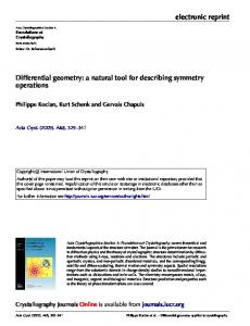
The eigenvalue may be positive or negative, we will use the Dirac sea representation, where all negative states are filled in the vacuum. On a plot of the eigenvalues ωn as a function of τ , the creation of a fermion is materialized by an energy level that goes out of the Dirac sea. Indeed, starting at ω(τ → −∞) < 0 the level is filled as it belongs to the Dirac sea. At the end of the transition τ → ∞, the energy of the level is positive ω(τ → ∞) > 0, and represents a particle, see Fig. 2.1. Let us consider the auxiliary problem −∂τ ΨL,R (τ, x) = HL,R (τ )ΨR,L (τ, x). (2.45) For adiabatically changing gauge fields, we already have a solution: Ψ(x, τ ) = e−

Rτ 0

dτ ωn (τ )

Ψn (x)

(2.46)

This solution is a zero-mode of the Euclidean Dirac equation (with τ = it) K(x, τ )Ψ = (∂τ + H(τ ))Ψ = EΨ.

(2.47)


16

E

Τ

Figure 2.1: Level crossing picture, one level crosses the zero-energy line and leads to the creation of one fermion.

It is normalizable from the fact that it crosses the zero-energy line. Indeed, Ψ(x, τ ) is normalizable at x → ±∞, because Ψ0 is, and vanishes at τ → ±∞ from the exponential factor in (2.46) as ωn is negative at τ → −∞ and positive at τ → ∞. To summarize, we connected the level crossing, and therefore the creation of one fermion, to the zero-modes of the Euclidean Dirac operator K. In a similar way, the creation of anti-fermions is represented by a level which crosses the zero-energy line from above. The construction (2.46) does not give a normalizable zero-mode for K, but it does give a zero mode for the operator K † (x, τ ) = (∂τ − H(τ )).

(2.48)

We observed that the number of created fermions can be found in the spectrum of the Euclidean Dirac Hamiltonian K. Combining this observation with Eq. (2.43) leads to the index theorem: e (2.49) ∆Nf = Ind(K) = d2 x εµν F µν , 2π where Ind(K) = dim(ker K) − dim(ker K † ).

2.4 2.4.1

The case of weak interactions Vacuum structure

We consider here a pure SU(2) theory with Higgs, L=

1 A 2 λ † 2 † µ 2 † d x − (Fµν ) + (Dµ H) (D H) + µ H H − (H H) , 4 2 3

(2.50)

2.4. THE CASE OF WEAK INTERACTIONS

17

where Dµ = ∂µ − igAaµ (T a H), T a = −iσ a /2 and σ a are the Pauli matrices. The electromagnetic U(1) is left aside4 . Weak interactions have the same complicated vacuum structure and topological properties as the Abelian Higgs model in 1+1 dimensions. We will therefore take several short-cuts in the derivations. The instanton counting goes as follows. As already explained, the finiteness of the action requires that on the points of the sphere S 3 at infinity, the fields are pure gauge. A gauge field configuration is a mapping from S 3 to SU(2). As π3 (SU(2)) = Z, these mappings can be separated in an infinite number of equivalence classes labeled by n ∈ Z. The equivalence classes are distinguished by the winding number: g2 a ˜ µν Fa , (2.51) Q= d4 xFµν 32π 2 where F˜ µν = 12 εµνρσ Fρσ is the Hodge dual field. As in 1+1 dimensions, Q = n when applied to a configuration of the equivalence class n. Rewriting the winding number as a surface integral leads to the Chern-Simons number: g2 2 abc a b c 3 a a εijk d x Fij Ak − ε Ai Aj Ak . NCS = 32π 2 3 It changes by n under application of large gauge transformations a a T 2πinx , U n = exp x2 + ρ2 where ρ is an arbitrary parameter of length dimension. There also are instanton and sphaleron transitions between vacua. The sphaleron solution cannot be written in analytic form and will be discussed in Chapter 6. For the instanton, see [16].

2.4.2

Fermionic content of the Standard Model and anomaly

The fermionic Lagrangian in the gauge basis reads Lf = Lγ µ DµLL + eR γ µ DµR eR + QL γ µ DµL QL + uR γ µ DµR uR + dR γ µ DµR dR √ 2 ˜ (2.52) + LMl eR H + QL KMd dR H + QL Mu uR H + h.c. , v α where L = Lα represents the leptonic left-handed doublets νeLα with α = e, µ, τ the L family index, eR =eαR represent the right-handed leptons, QL = Qαc L the left handed uαc L quark doublets dαc , c being the color index c = 1, 2, 3. The right handed quarks are L ˜ = −H∗0∗ . The matrices denoted uαc and dαc , the Higgs doublet is H = H1 and H R

R

H0

H1

Ml , Md , Mu are the diagonal and real mass matrices for the leptons, down quarks and up quarks and K is the Cabibbo-Kobayashi-Maskawa matrix, which contains the mixing 4

In the computation of the sphaleron rate, we explain in Appendix L how to take the electromagnetic sector into account.


18

angles between quarks and a CP violating phase. The covariant derivatives contain terms from electrodynamic and strong interactions, which will not be given here, and a term for the weak interactions for the left components, DµL = ∂µ − ieAaµ T a , DµR = ∂µ . The current associated with the 12 left-handed doublets ψLi = {qLαc , Lα } suffer from an anomaly. Triangle diagrams containing interactions with a weak field background lead i to the nonconservation of the fermion number current Jµ = ψ L γµ ψLi so that g2 ∂ Jµ = 12 32π 2

µ

a ˜ µν Fa . d4 xFµν

(2.53)

The right-hand side of this equation matches the winding number (2.51), that is to say that if the gauge fields change from one vacuum state to the next one (Q = 1), twelve fermions are created. Since the process may go in any direction, no net fermion number creation arises from this mechanism alone. Keeping in mind the properties of the electroweak theory, we will now build a 1+1 model, which imitates the electroweak nonperturbative physics as closely as possible.

2.5

A two dimensional model of the electroweak theory

We describe here the model that will be studied in the next three chapters and explain the common properties it shares with the electroweak theory. We also give a short review of the existing 1+1 dimensional models, with some of their properties in Appendix A. The model we will study contains a complex scalar field φ with vacuum expectation value v; a vector field Aµ , and nf fermions Ψj , j = 1, ..., nf : e 1 j L = − F µν Fµν + iΨ γ µ (∂µ − i γ 5 Aµ )Ψj 4 2 1 j 1 − γ5 j 2 j j 1 + γ5 j ∗ Ψ φ − if j Ψ Ψ φ. −V (φ) + |Dµ φ| + if Ψ 2 2 2

(2.54)

The charges of the left- and right-handed fermions differ by a sign, eL = −eR = 2e , and the symmetry breaking potential is chosen to be V [φ] = λ4 (|φ|2 − v 2 )2 . The particle spectrum consists of a Higgs field with mass m2H = 2λv 2 , a vector boson of mass mW = ev, and nf Dirac fermions acquiring a mass F j = f j v via Yukawa coupling. The model is free from gauge anomaly.5 There is, however, a chiral anomaly leading to the nonconservation of the fermionic current, Jµ =

JµL

+

JµR

=

nf

j=1

5

j ΨL γµ ΨjL

+

nf

j=1

j ΨR γµ ΨjR

=

nf

j

Ψ γ µ Ψj ,

j=1

Gauge anomaly spoils the renormalizability of the theory. It is canceled here by the choice of charges for the left and right component of the spinor. It is not possible to have only left-handed fermions that are charged, like in the electroweak theory, and still have fermion number nonconservation.

2.6. CONFINEMENT PROBLEMS IN 1+1 DIMENSIONS

19

with a divergence given by ∂µ Jµ = ∂µ JµL + ∂µ JµR = −nf

eL eR e εµν Fµν + nf εµν Fµν = −nf εµν Fµν . 4π 4π 4π

(2.55)

As we have seen in Sec. 2.1, the vacuum structure of this model is non-trivial. The transition between two neighboring vacua leads to the nonconservation of fermion number by nf units, as in the electroweak theory. This model, or very similar ones, have been studied as toy models for the fermionic number nonconservation in the electroweak theory in a number of papers; see, e.g. [43, 44]. Note that we do not reduce generality in considering Yukawa interaction between identical fermions only6 . In principle another mass term of the form MΨT γ0 Ψ+h. c. could be added to the Lagrangian (2.54). It is compatible with gauge and Lorentz invariance but breaks fermion number explicitly. As we are interested in instanton mediated fermion number nonconservation, we will not consider this term. In Chapter 3 we consider nf to be even. The case of odd nf , resulting in the creation of an odd number of fermions, is analyzed in Chapter 4. In Chapter 5 new particles and some more interaction terms will be added to understand the effect of the interactions between fermions.

2.6

Confinement problems in 1+1 dimensions

Two dimensional models display some strange properties, which are very interesting on their own, but may be a disaster for our purposes. We will explain what they are, where they occur and see that the precise model we want to study is free from such undesired effects.

2.6.1

Confinement of fermions by instanton gas

It is well known that in some 1+1 dimensional Abelian models, for instance in the theory defined by (2.1), non-integer charges q (we will call them quarks) are confined [33, 34]. Since one of our aims is to show that the 1+1 dimensional theory allows for the creation of one single fermion, confinement would be a serious problem. We already stress that this does not apply to our half charged fermions but this point needs to be discussed. A well known derivation of this involves Wilson loops (see for instance [33, 34]). It needs to consider two charged particles separated by a distance L. Instantons present between the two particles lead to an attractive force F . In the dilute instanton gas approximation7 it reads (2.56) F = −2κe−S0 (cos[θ] − cos[θ + 2πq/e]) i j ∗ 5 ˜ij A more general interaction could be written in the form if˜ij Ψ 1+γ 2 Ψ φ + h.c. but the matrix f j can always be diagonalized and made real through redefinition of the fields Ψ . 7 This approximation means instantons are rare events such that the particle will never hit any instanton core, only interactions with the instanton tail are taken into account 6


20

where S0 is the classical action, θ is the vacuum angle and κ contains the one loop quantum corrections. Note that the force is attractive and independent of the charge separation. This derivation leads directly to the static interaction potential, however, it is not Lorentz invariant, and requires that the charges “holds” at some place in spite of the attractive confining force. We will present here an original alternative derivation, which does not have these drawbacks and does not require any supplementary approximation. It is also closer to what we want to check, since it is based on the evolution of a single particle. We consider a quark of mass M moving in a space of length L. We want to compute its full propagator (2.57) G(x, y) = θ|T Ψ(x)Ψ(y) |θ, where Ψ is the quark field. In Euclidean space setting y = 0, it is a solution of the equation (2.58) −iγµE (∂µ − iqAµ ) − M GE (x) = δ(x). To solve this equation, we will choose a very particular gauge. The idea is to gauge rotate the instanton asymptotic fields (2.17) to a particularly simple form. For instance on the instanton solution (2.19) with winding number n expressed in the Ar = 0 gauge, we apply the gauge transformation x0 x0 (2.59) α = n −atan θ(x0 ) + atan − θ(−x0 ) . x1 x1 This leads to the following form for the gauge field far from the instanton center: n A0 = −2π δ(x0 )θ(−x1 ), q

A1 = 0.

(2.60)

In the instanton gas we consider, we combine different gauge transformations (2.59) to deform all the asymptotic instanton fields to lines in the negative direction of the space axis. We shall first find how a particle propagates in the field of an instanton centered at a = (a0 , a1 ). We use the following ansatz for the Green’s function (2.57), G(xµ ) = f (x0 )g(x1 )G0 (xµ ), where G0 (x) is the free propagator. The differential equation (2.58) in the field configuration (2.60) can be solved for the function f and g, q

g(x1 ) = 1 f (x0 ) = e−2πin e θ(x0 −a0 ) .

(2.61)

The effect of the instanton asymptotic fields is to give a phase to the free propagator. This solution can be generalized to the case of many instantons at positions ai , i = 1, ..., ninst. The effect of a dilute instanton gas is found performing an average on all possible instanton and anti-instanton configurations8 , weighted by their probability of occurrence e−S0 κT L, where L is the size of the space and T = x0 − y0 the interval of time considered. Different cases need to be distinguished. The particle can pass trough a number (n) of instanton or 8

We disregard instantons with higher winding number. They have a larger action, therefore their probability is exponentially suppressed.

2.6. CONFINEMENT PROBLEMS IN 1+1 DIMENSIONS

21

¯ ) to the instanton core9 . The anti-instanton (¯ n) and it can pass left (n, n ¯ ) or right (n , n propagator is then expressed as a sum over n, n , n ¯, n ¯ , which represent all the different possible configurations: (n+¯n+n +¯n )

q 1 L −S0 e κT e2πi(¯n−n) e eiθ(n+n −¯n−¯n ) G0 (x) G(x) = n!n !¯ n!¯ n! 2 n,n ,¯ n,¯ n L q −S0 (2.62) = exp e κT cos θ − 2π − cos θ G0 (x). 2 e Back to Minkowski space, the exponential in (2.62) is imaginary and corresponds to a mass term. By Fourier transforming back to momentum space, we find the mass 2 L q cos θ − 2π − cos θ m2f = M 2 + e−S0 κT 2 e for the quark. It diverges for L → ∞, which means that a single charged state cannot exist. Till now we made no assumption on the exact nature of the quark. If we take a chiral fermion (of charge q) as in (2.32, 2.41), we may find another conclusion. Indeed the constant κ contains the determinant of the Euclidean Dirac operator K, which may contain a zero-mode. It is the case in the model of interest 2.54 and the above argument fails.

2.6.2

Confinement of instantons by fermions.

A common statement [34] is that tunneling is suppressed by massless fermions. This statement also applies to the model (2.54), but needs to be interpreted correctly. The presence of massless fermions modifies the tunneling probability (2.21) in the following way: The fermionic fluctuation determinant should be included to the factor κ, which also contains the determinants of the bosonic fluctuation operators. We know from (2.49) that the fermions possess zero-modes10 , therefore the fermionic determinant vanishes and so does the transition probability (2.21). For instance massless fermions liberate the quarks from the previous section [45], as the confinement force (2.56) is proportional to κ. More precisely, although the instanton contribution to the partition function |θ|e−Hτ |θ is suppressed as asymptotic process (τ → ∞), it is allowed locally. Indeed, the fermionic spectrum possesses an exact zero-mode only in the infinite space limit. If the instanton transition is closely followed by an anti-instanton, no exact zero-mode exists and such processes are allowed. This suggests that there exists a confining force11 between instantons and anti-instantons (separated by a distance R), which prevents global tunneling [46, 47]. Indeed we can rewrite the fermionic determinant as an effective potential 9

In the dilute gas approximation we neglect the probability of passing through the instanton core. The index theorem given in (2.49) holds for chiral fermions, but a similar theorem can be written [32] for vector fermions and also leads to the presence of zero-modes. 11 The term “force” is somewhat abusive since we are in Euclidean space. 10


22

Vfone loop = ln(det(K)) for the bosonic action. For massless fermions, an analytical calculation gives [48]: 2 ln((det(K)) = −e (2.63) d2 xA2µ . For an instanton anti-instanton configuration, we have −e2 d2 xA2µ ∝ ln(eR), which leads to the existence of an attractive force F ∝ R1 . If the fermions are coupled to the Higgs field (and acquire a mass mf ), as in (2.54), the zero-modes exist and the instantons are also confined. The confining potential is indeed even stronger; in this case (see Appendix E, equation (E.7)), Vfone

loop

∝ −mf R,

(2.64)

which is the sign of a constant force between instantons. The vanishing probability of the vacuum to vacuum transition by one instanton |θ|e−Hτ |θone instanton = 0 is not a problem for our purposes. Indeed it means that fermions have to be created in an instanton transition [16]. We will see that an instanton transition has non-zero probability if it is accompanied by the emission of N fermions for each N present zero-modes. The Green’s function |θ|e−Hτ ψ 1 . . . ψ N |θone instanton in path integral formalism reads (2.65) DψDψDAµ Dηe−S[ψ,ψ,Aµ ,η] ψ 1 . . . ψ N , where the η stands for all other eventual degrees of freedom as the Higgs field. Using the conventional Grassmann properties of the fermionic path integral and performing the Gaussian integral around the instanton solution, we find (see Chapter 3 for more details) |θ|e−Hτ ψ 1 . . . ψ N |θone

instanton

2 = e−S0 τ L det−1/2 (Dbos ) det (K),

(2.66)

2 where det−1/2 (Dbos ) represents the product of the determinants of all bosonic degrees 12 of freedom and det (K) represents the fermionic determinant with all zero eigenvalues omitted. The result (2.66) for the transition probability is in principle non-zero, as long as we introduce as many fermionic operators as needed to cancel each zero-eigenvalue. Transitions between different sectors |n are possible, if they are accompanied with the emission or annihilation of fermions. Such events, are strictly speaking not vacuum to vacuum transitions. However it can be shown that, even in this case, the θ-vacua are still the correct vacua of the theory [17]. As we have seen, anomalies arise at one loop order [49]. To put the claims made in this chapter on firmer grounds, a complete control of the one-loop corrections is needed. In the path integral formalism, one-loop corrections are all included in the determinant of the fluctuation operators. The determinant of the bosonic operators were calculated in Ref. [50] and the fermionic determinant will be computed in the following chapter. 12

With zero-eigenvalue replaced by the normalization factors coming from the variable change to collective coordinates.

Chapter 3 Fermionic determinant In this chapter, we compute the one-loop fermionic contribution to the probability of an instanton transition with fermion number violation in the chiral Abelian Higgs model in 1+1 dimensions. The one-loop contributions are expressed through the determinant of the fermionic fluctuation operator. The dependence of the determinant on fermionic Yukawa couplings, scalar and vector mass is determined.

3.1

Introduction

The interest in the chiral Abelian Higgs model in 1+1 dimensions lies in the fact that it shares some properties with the electroweak theory but is much simpler and may serve as a toy model. One of the most interesting common features of the two gauge theories is the fermionic number nonconservation [16]. Both give rise to instanton transitions, leading to the creation of a net fermion number due to an anomaly [13, 15]. Both theories contain finite temperature sphaleron transitions [19, 43]. At zero temperature, zero fermionic chemical potentials and for a small number of particles participating in the reaction, the probability of the process can be computed using semiclassical methods. In general, the result is a product of the exponential of the classical action e−Scl and the fluctuation determinants. The latter factor includes the small perturbations of the fields around the instanton configuration and, in many cases, may be computed only numerically. Quite a number of computations of determinants in 1+1 dimensions can be found in the literature.1 In particular, the determinants have been calculated for the vector and scalar field fluctuations around the instanton in Ref. [50], as well as for the fermionic ones in Ref. [59], where it was assumed that fermions have no mass term and no interaction with the Higgs field. However, to our best knowledge, no computations incorporating the Yukawa coupling of the fermions to scalar field have been done until now, neither for realistic case of electroweak theory nor for the chiral Abelian Higgs model.2 1

For 3+1 dimensional computation without Yukawa couplings see the seminal paper by ’t Hooft [16]. The determinants in the high temperature sphaleron transition in 1+1 dimensions were computed in [43]. 2

23

CHAPTER 3. FERMIONIC DETERMINANT

24

The aim of the present work is to partially fill this gap, calculating the fermionic determinant in the 1+1 dimensional case, where the fermions interact with the Higgs field in a similar way as in the electroweak theory 3 . This calculation is somewhat delicate because of the difficulties occurring in regularization and renormalization of chiral gauge models beyond perturbation theory. Furthermore, an analytic solution to this problem cannot be obtained, since even the classical instanton profile, given by the Nielsen-Olesen string solution [38], is not known analytically, apart from the special case where the Higgs mass equals the vector field mass [62]. Nevertheless, we use analytical methods as long as possible before moving on to numerical computation. We will use a numerical method developed in [63], extended to our case. The chapter is organized as follows. In Sec. 3.2, the model and its basic features, such as its vacuum structure, anomaly, instanton configuration, and fermionic zero modes, are discussed. In Sec. 3.3, we study and compare the 1-loop divergences occurring in this model in various regularization schemes. In Sec. 3.4, the method of Ref. [63] to calculate determinants is discussed and applied to our case. In Sec. 3.5 we present in some detail the numerical procedures and give the results of the determinant computation. Finally, conclusions are given in Sec. 3.6.

3.2

The model

We consider the model given by the Lagrangian (2.54), which contains a complex scalar field φ with vacuum expectation value v; a vector field Aµ , and nf fermions Ψj , j = 1, ..., nf . We restrict ourselves to the case of an even number of fermions nf . We recall the fermionic Lagrangian and some of its properties: e j j 1 + γ5 j ∗ j 1 − γ5 j Ψ φ − if j Ψ Ψ φ. (3.1) Lf = +iΨ γ µ (∂µ − i γ 5 Aµ )Ψj + if j Ψ 2 2 2 The vacuum structure of this model is nontrivial [17]. Taking the A0 = 0 gauge and putting the theory in a spatial box of length L with periodic boundary conditions, one finds that there is an infinity of degenerate vacuum states |n, n ∈ Z with the gauge-Higgs configurations given by 2πnx 2πn (3.2) A1 = , φ = vei L . eL The transition between two neighboring vacua, described by an instanton, leads to the nonconservation of fermion number by nf units.

3.2.1

Lagrangian in Euclidean space

As the tunneling is best described in Euclidean space-time, we review here the corresponding equations and conventions. The Lagrangian (3.1, 2.54) may be rewritten in Euclidean 3

Similar studies have recently been performed for other models. In a supersymmetric theory in 2+1 dimensions the calculation is simplified by a supersymmetric constraint [60]. The fermionic contribution to the vortex mass has been calculated in a model resembling the (nonchiral) Abelian Higgs gauge theory, where the fermion couples to the absolute value of the scalar field [61].

3.2. THE MODEL

25

space: LE =

1 e j Fµν Fµν + iΨ γµE (∂µ − i γ5 Aµ )Ψj + V (φ) 4 2 1 j 1 − γ5 j † j j 1 + γ5 j ∗ + (Dµ φ) (Dµ φ) − if Ψ Ψ φ + if j Ψ Ψ φ, 2 2 2

(3.3)

with Dµ = ∂µ − ieAµ , γ0E = iγ0 and γ1E = γ1 . The fields Ψ and Ψ are independent variables, and the gauge transformation reads: γ5

γ5

Ψ −→ eiα(x) 2 Ψ , Ψ −→ Ψeiα(x) 2 , φ −→ eiα(x) φ.

(3.4)

For comparison, the Lorentz transformation is: Ψ(x) → Ψ (x ) = Λs Ψ(Λ−1 x ),

−1 Ψ(x) → Ψ (x ) = ΨΛ−1 s (Λ x ),

with Λs = exp(iγ 5 θ2 ) being the rotation matrix in two dimensions.

3.2.2

Instanton

The instanton which describes the tunneling between the states |0 and |n is simply the Nielsen-Olesen vortex with winding number n [38], which is a solution of the Euclidean equations of motion in two dimensions. In polar coordinates (r, θ), the field configuration reads: φ(r, θ) = einθ φ(r) = einθ vf (r),

(3.5)

Ai (r, θ) = εij rj A(r),

(3.6)

where r is the unit vector r = (cos θ, sin θ) and εij the completely antisymmetric tensor with ε01 = 1. The functions A and f have to satisfy the following limits: f (r) −→ cr |n| , r→0

r→∞

f (r) −→ 1, r→0

A(r) −→ 0,

(3.7)

n A(r) −→ − . er r→∞

Passing to dimensionless variables A=

m˜ A, e

φ=

m˜ φ, e

r=

r˜ m

with m =

√

λv 2

˜ φ˜ are : reduces the number of free parameters. The equations for A, 1 1 2 ˜ − ˜ ∂r˜rÃ(r) = 0, + φ˜ A(r) −∂r˜ r˜ r˜ 2 1 1 ˜ 2 2 ˜ ˜ ˜ − ∂r˜ r˜∂r˜φ(r) + − A(r) − 1 + µ φ(r) φ(r) = 0, r˜ r˜

(3.8)

(3.9)


26

with µ2 =

m2H 2m2W

=

λ . e2

The classical action is given by:

∞

Scl = πv 2 + µ2

0

 

r˜d˜ r µ2 

˜ A(r) A˜ (r) + r˜

2 (3.10)

2 2 4 µ 1 1 ˜ 2 A(r) ˜ − φ˜ (r)2 + φ(r) + . φ˜2 (r) − 2 r˜ 2 µ

The number ∆N of fermions created in the instanton transition can be computed by integrating (2.55) over the Euclidean space:

∆N = −

d x∂µ Jµ = −nf 2

d2 x

e εµν Fµν = −qnf , 4π

(3.11)

e where q = d2 x 4π εµν Fµν is the winding number of the gauge field configuration. For the instanton configuration (3.5,3.6), we have q = n.

3.2.3

Fermionic zero modes

According to the index theorem (see, for example, [32]), the Dirac operator in the background of the instanton satisfies the following relation: dim ker[K] − dim ker[K † ] = n. As the instanton in 1+1 dimensions coincides with the vortex, these zero modes may be found by carrying out a similar analysis as in Ref. [66], where the fermionic zero modes on the Nielsen-Olesen string were analyzed for nonchiral fermions. In this subsection, we present the corresponding equations. The Lagrangian for the fermion j in the background of the scalar and vector fields j j j may be written as LE fj = Ψ K Ψ , where j

K =

−if j φ∗ i∂0 − 2e A0 − ∂1 − i 2e A1 e e −i∂0 − 2 A0 − ∂1 + i 2 A1 if j φ

.

(3.12)

In the following, the family dependent Yukawa coupling f j will be replaced by f , keeping in mind that there is no mixing between different fermionic generations. The zero modes are the regular normalizable solutions of the equation KΨ = 0, with Aµ and φ given by (3.5, 3.6) 4 . Using polar coordinates and performing the substitution ˜ = exp r A(ρ) dρ Ψ, we get: Ψ 0

2

4

∂ ∂ + ri ∂θ −iF f(r)e−inθ ieiθ ∂r ˜ = 0, Ψ ∂ ∂ iF f (r)einθ − ri ∂θ −ie−iθ ∂r

(3.13)

However, in the massless case (f j = 0), a logarithmically divergent wave function is generally kept as a relevant solution. The reason is that its classical action is finite [44].

3.2. THE MODEL

27

˜ = where F = f v is the fermion mass. With the use of the phase decomposition Ψ ∞ imθ m Ψ , Eq. (3.13) can be rewritten as m=−∞ e ∂ m−n−1 m − F f (r)ΨL − = 0, Ψm−n−1 R ∂r r ∂ m m−n−1 + Ψm = 0. (3.14) L − F f (r)ΨR ∂r r In our case, the analysis of Ref. [66] shows that for a vortex with topological number n < 0 there are exactly |n| fermionic zero modes in the spectrum of K with m in the interval m ∈ {−n + 1, .., 1, 0} and none in the spectrum of K † . For n > 0 there are no zero modes in the spectrum of K, but n in the spectrum of K † . For the case of n = −1 studied below, the explicit form of the zero mode is given by r e 0 0 ΨL (r) = ΨR (r) ∝ exp − (3.15) F f (r ) + A(r ) dr . 2 0 Note that for massless fermions (F = 0), the zero mode decreases as √1r for large r. It is therefore not normalizable and has a divergent action. This behavior differs form the case of Refs. [59, 48, 44], where massless fermions of charges e were considered. In their case, the fermionic zero mode decreases as 1r for large r and has a finite action.

3.2.4

Determinant

Because of the presence of the fermionic zero modes, instanton transitions imply the creation of a net number of fermions. In the following, we will be interested in the creation of one of each type of fermion, for which an instanton of charge n = −1 is needed. The corresponding transition probability is proportional to det K, where the prime means omission of the zero eigenvalue in the calculation of the determinant. It is well known [16] that the eigenvalue problem for the operator K is ill defined. Consequently, one has to consider the Laplacian type operators K † K or KK † , which have the same set of eigenvalues (except for the zero modes). Then det K is defined up to a phase as det [K] = det [K † K]1/2 . The explicit expression for the operator K † K reads: (3.16) K †K = 2 −if [φ(eA0 + ieA1 ) + (i∂0 − ∂1 )φ] f |φ(r)|2 − (∂µ − i 2e Aµ )2 + 2e µν ∂µ Aν . if [φ∗ (eA0 − ieA1 ) − (i∂0 + ∂1 )φ∗ ] f 2 |φ(r)|2 − (∂µ + i 2e Aµ )2 + 2e µν ∂µ Aν The fermionic equations of motion, for instance Eq. (3.13), remain unchanged after the variable changes (3.8), if f is replaced by f /e and e is set to 1. The only free parameter in the bosonic sector (3.10) is µ, while there is a second parameter in the fermionic sector: the Yukawa coupling f . In conclusion, we are left with two dimensionless parameters, and the determinant can be calculated as a function of √ F f mW f mH (3.17) = µ 2 and = =√ . mW mH e mH 2λ


28

Obviously the determinant, being a product of an infinite number of eigenvalues, is a divergent quantity. In the next section, we discuss its regularization and renormalization.

3.3

Regularization and renormalization

For perturbative calculations, the dimensional regularization is best suited. However, as has been observed in Ref. [16], it is not applicable to the computation of the fermionic determinant, because the continuation of the instanton fields to a space with a fractional number of dimensions is not uniquely defined. Nevertheless, we discuss the dimensional regularization to fix the meaning of the Lagrangian parameters in Sec. 3.3.1. In Sec 3.3.2, we consider another regularization scheme based on partial waves decomposition. It permits one to exploit the spherical symmetry and turns out to be convenient for numerical purposes. In Appendix A, we consider the Pauli-Villars regularization used in Ref. [16] and prove its equivalence with the partial waves procedure.

3.3.1

Dimensional regularization

The Lagrangian depends on four parameters: the charge e, the scalar coupling λ, the scalar mass mH , and the Yukawa coupling f . The model under consideration is superrenormalizable. In order to use the dimensional regularization, we have to define the γ-matrices for an arbitrary number d = 2 − ε of dimensions: {γ µ , γ ν } = 2g µν , µ, ν = 0, 1, ..., d − 1.

tr(γ µ γ ν ) = 2g µν ,

(3.18)

The definition of the γ 5 matrix is ambiguous, we follow here the usual definition: 5 ν γ ,γ = 0, 5 ν = 0, γ ,γ

ν = 0, 1. ν = 2, ..., d − 1.

(3.19)

The physical parameters e, λ, mH , f in two dimensions are related to the d-dimensional parameters ed , λd , mHd , fd by: d

ed = eµ1− 2 ,

λd = λµ2−d ,

d

mHd = mH µ1− 2 ,

d

fd = f µ1− 2 .

We will work in the Rξ gauge. The complex field φ is written as φ = v + h + iϕ, where h and ϕ are real. The gauge fixing term is 1 Lg.f. = d2 x G[A, h, ϕ]2 , (3.20) 2 where G[A, h, ϕ] =

1 (∂µ Aµ − ξevϕ) . ξ

(3.21)

3.3. REGULARIZATION AND RENORMALIZATION

29

The Lagrangian for ghost fields c is

h d x¯ c −∂ − ξe v 1 + c. v

Lghost =

2

2

2 2

(3.22)

In the following we will work in the minimal subtraction (MS) scheme. The only divergent parameter is the Higgs mass mH . A straightforward computation gives the relevant part of the effective action, 1 UV Scount = dd x φ2 − v 2 δm2 (3.23) 2 with 1 1 1 µ2 µ2 2 ln( 2 ) + + λ−e δm = 3λ ln( 2 ) + 4π mH ε MS mW ε MS 1 µ2 2 −2f ln( 2 ) + , F ε MS 2

where 1ε M S = counterterm

1 ε

(3.24)

− γ + ln(4π). In the minimal subtraction scheme, we subtract the

1 2 φ − v 2 δm2M S , 2 with δm2M S containing all terms in (3.24) proportional to 1ε M S . For the photon propagator, the bosonic loops do not introduce any renormalization. However, as is well known [32], there is a finite contribution coming from fermionic loops. Because of the ambiguities in the definition of γ5 , dimensional regularization breaks the e chiral gauge invariance, and a term 4π A2µ needs to be added to the action. The complete counterterm action to be subtracted from the initial action (3.3) reads: UV Scount

d2 x

e 1 2 φ − v 2 δm2M S d x − A2µ + 4π 2

d

Scount =

3.3.2

=

.

(3.25)

Partial wave regularization

The spherical symmetry of the instanton suggests that partial wave expansion can be used. The eigenvalue problem decouples into one-dimensional differential equations. In this section, we discuss a natural way to regularize the partial waves. We consider here only the fermionic sector. Partial wave expansion We may write det[K † K] as a path integral: †

det[K K] =

DηD η¯ exp

2

†

d x η¯K Kη .

(3.26)


30

Partial wave decomposition is defined as follows: ∞

η(r, θ) =

imθ m

e

η (r),

∞

η¯(r, θ) =

m=−∞

e−imθ η¯m (r).

(3.27)

m=−∞

The regularization is done by putting our system in a finite spherical box of radius R, and cutting the sum over the partial waves at some m = L. After performing the partial wave decomposition, the regularized action reads:

R

2πr dr

S(R, L) = 0

M

η¯m (r)M ml (r)η l (r),

(3.28)

m,l=−L

with ml

L

1 = 2π

dθe−imθ K † Keilθ .

(3.29)

From the general expression (3.17) for K † K, we get for the vacuum: †

K Kvac =

F 2 − ∂02 − ∂12 0 2 0 F − ∂02 − ∂12

.

(3.30)

After phase decomposition we obtain a diagonal matrix in both spinor and partial wave space: m2 1 ∂ ∂2 ml ml 2 + 2 +F , (3.31) Mvac = δ 1l2 − 2 − ∂r r ∂r r where 1l2 is the identity in spinor space. The radial eigenvalue equation in vacuum reads: mm m ηλ = λ2 ηλm , Mvac

(3.32)

with boundary conditions η m (0) = η m (R) = 0, 0

η (0) = 1,

m = 0,

0

η (R) = 0.

(3.33)

From the relations (3.31)-(3.33) the free propagator may be derived GR m (r, r ) =

η¯m (r)η m(r ) λ

λ

=

1l 2π

λ

λ2 Im (F r) [Km (F r )Im (F R) Im (F R) Im (F r ) [Km (F r)Im (F R) Im (F R)

− Im (F r )Km (F R)] ,

r < r,

− Im (F r)Km(F R)] ,

r > r.

(3.34)

It allows us to treat the interaction terms present in (3.17) by standard diagrammatic methods.

3.3. REGULARIZATION AND RENORMALIZATION

31

One-loop divergences in partial waves As we have already seen, the fermionic parameter f needs no renormalization. However, the mass of the scalar Higgs receives divergent contributions from fermionic diagrams. The partial wave regularization can’t be introduced at the level of the fermionic Lagrangian (3.3), but only at the level of the squared determinant (3.26). One does not expect that the counterterms derived from the initial Lagrangian are sufficient to remove all infinities in (3.26). Hence, we recalculate the counterterm action (see Appendix C for details) needed to renormalize (3.26). The result is: UV (L, R) = Scount

L

m Scount (R)

m=−L

=

L

m=−L

0

R

e 2πr tr[Gm (r, r)] f 2 |φ|2 − v 2 + εµν ∂µ Aν dr, (3.35) 2

m are finite for each m and only the sum is divergent in the limit L → ∞. where the Scount Note that the counterterm (3.35) is non-local. This is due to the non-locality of the partial wave regularization procedure and may be checked to be correct by comparison to Pauli-Villars regularization, see Appendix B.6. For small constant background fields, (3.35) leads to R e 4L2 UV 2 2 2 2 1 f |φ(r)| − v + εµν ∂µ Aν (r) d r 1 + log .(3.36) Scount = 2 2π F 2 R2 0

In order to get results in the MS scheme from those calculated in the partial waves, we UV between the effective action found in these two schemes.5 calculate the difference δScount The result reads 2 4L2 1 dx 2 UV f (|φ|2 − v 2 ) + Sgf , δScount = log (3.37) − 2 2 Rµ ε MS 2π 2 4L2 d xe νρ ∂ν Aρ (x). Sgf = log (3.38) R2 F 2 2π 2 In comparison with the dimensional regularization, a supplementary divergent term involving gauge fields Sgf has appeared. It also arises when using Pauli-Villars scheme (see Appendix B.3) and is an extra divergence of the action (3.26) in comparison to the initial action (3.3). If we Wick-rotate Sgf back to our initial Lagrangian in Minkowski space-time, it gets an extra factor of i, and the action becomes non-hermitian and breaks unitarity. Because of this, Sgf must be subtracted completely. For the photon propagator, as in dimensional regularization, we have to subtract from the effective action the term e2 R 2 2 IR d rA (r) (3.39) Scount (R) = 4π 0

where

5

The counterterms found in the dimensional regularization have to be multiplied by a factor of 2, because we are dealing here with the squared operator K † K.


32

to recover chiral gauge invariance (see Appendix C.1). Regularization and renormalization in partial waves From the counterterm (3.36), we see that the initial theory is recovered in the limit 2L → ∞. The summation over partial waves and the limit L → ∞ has to be performed FR first and the infinite volume limit must be taken only after having removed the infrared counterterm. The explicit expression for the counterterms in the case of space dependent background is obtained in integrating (3.35) and the renormalized fermionic determinant may formally be written as: detren [K † K] = (3.40) ! L # " det[M m ] UV IR inst exp −Scount lim (L, R) exp −Scount (R) lim . m R→∞ L→∞ det[M ] vac m=−L This prescription differs from the one of [63] where the limit R → ∞ is taken first. It is shown in Appendix C that the order of the limits is crucial.

3.4

Determinant calculation

After the partial wave decomposition (3.26-3.29), K † K(r, θ) was expressed in terms of M lm (r). For our purposes, the case where M lm is diagonal in partial wave space (M lm = δlm M m ) is sufficient6 . The determinant may be calculated as: †

det[K K] =

+∞ "

det[M m ].

(3.41)

m=−∞

We are left with the much easier problem of finding the determinant of one-dimensional operators, which may be addressed with the following theorem [33]: Let us consider two operators Oi = −∂x2 + Wi (x), i = 1, 2 defined in an interval of length R. Let Ψi , i = 1, 2 be the solution of Oi Ψi = 0 with the boundary conditions Ψi (0) = 0, Ψi(0) = 1, i = 1, 2, we have:

6

(3.42)

O1 Ψ1 (R) det = . O2 Ψ2 (R)

(3.43)

We are interested mainly in the case n = −1, where one of each type of fermions is created. In this ml particular case, the operator Minst is diagonal in partial wave space. Note that this point is not crucial, as explained in Sec. 3.4.1, the determinant may be calculated in the nondiagonal case as well.

3.4. DETERMINANT CALCULATION

3.4.1

33

Treatment of radial operators

We follow here the method developed in Ref. [63] to calculate determinants. Note that here we will first consider the radial problem for 0 to R where R 1 and the limit R → ∞ will be taken afterward. In the present case, even if M ml is diagonal in partial wave space, it is not diagonal in spinor space. The theorem (3.43) needs generalization to two coupled second order differential equations. We are interested in the ratio between the operator m m M11 M12 m M = m m M21 M22 in the instanton background and the vacuum operator M m,vac , which is assumed to be m,vac diagonal. Let us define the matrix ψijm (i, j = 1, 2) and ψL,R as the solutions of the following differential systems: n,vac m,vac m M m ψj1 = 0, M11 ΨL = 0, j ij m (3.44) n,vac m,vac ΨR = 0, j Mij ψj2 = 0, M22 with boundary conditions m ψ11 vac,m = 1, r→0 ψ L m ψ12 lim vac,m = 0, r→0 ψ L

lim

m ψ21 vac,m = 0, r→0 ψ R m ψ22 lim vac,m = 1. r→0 ψ R

lim

(3.45)

The determinant is then given by: det[ψijm (R)] det[M m ] = m,vac . det[M m,vac ] ψL (R)ψRm,vac (R)

(3.46)

The remaining determinant is just the usual determinant for 2 × 2 matrices. It is an easy exercise to reproduce step by step the demonstration of Ref. [33] in this more general case. = The vacuum operator which is given in (3.31) has an analytic solution Ψm,vac j Im (F r). For the instanton (n = −1) configuration, we get: m2 ∂2 1 ∂ e e2 2 A(r) 2 2 + ε A (r) + me , − + F f (r) + ∂ A + µν µ ν 2 2 ∂r r∂r r 2 4 r 1 m = M21 = F −f (r) − f (r) + eA(r)f (r) , r 2 2 ∂ 1 ∂ e e2 2 A(r) m 2 2 = − 2− + 2 + F f (r) + εµν ∂µ Aν + A (r) − me . (3.47) ∂r r ∂r r 2 4 r

m M11 = − m M12

M22

The solution Ψm ij (r) needs to be computed numerically. To this aim, it is convenient to make the following substitution: m (r) = δ + h (r) Im (r), (3.48) Ψm ij ij ij


34

The determinant is then evaluated with det[M m ] = det[δij + hm ij (R)]. vac,m det[M ]

(3.49)

In terms of the functions hm ij , the equation (3.44) takes the form of an ordinary quantum mechanical equation with potential Vij (r): 2 1 ∂ (F r) ∂ Im m m + (r) = V (r) δ + h (r) . (3.50) + 2 h ik kj ij kj ∂r 2 r Im (F r) ∂r The effective potential Vij (r) in the background of the instanton is given by the following expressions: A (r) A(r) A2 (r) A(r) + e2 −e − me , V11 (r) = F 2 f 2 (r) − 1 − e 2r 4 2 r F f (r) V12 (r) = V21 (r) = eF f (r)A(r) − F f (r) − , r A (r) A(r) A2 (r) A(r) + e2 −e + me . V22 (r) = F 2 f 2 (r) − 1 − e 2r 4 2 r

(3.51)

The functions hm ij (r) can easily be found numerically from (3.50) with the boundary conditions hij (0) = 0, i, j = 1, 2, (3.52) hij (0) = 0, i, j = 1, 2. 0 . In this case, it is possible For m = 0 we have to remove the zero-mode present in Minst m to diagonalize the operator Minst with the substitution Ψ± = ΨL ± ΨR : ∂2 1 ∂ e e2 − 2− + F 2 f 2 (r) + εµν ∂µ Aν + A2 (r) ∂r r ∂r 2 4 1 (3.53) ± F −f (r) − f (r) + eA(r)f (r) Ψ± = M±0 Ψ± = 0. r

The fermionic zero-mode is contained in M+0 . We calculate det[M−0 ] with (3.43) and det [M+0 ] as in Ref. [63]: det [M+0,inst ] = det[M+0,vac ]

d det[M+0,inst + λ2 ]|λ2 =0 dλ2 det[M+0,vac ]

=

d λ h (R). dλ2

(3.54)

vac In the last relation hλ (r) is defined through Ψinst (1 + hλ ) with Ψinst +λ = Ψ +λ (r) being a solution of (M+0,inst + λ2 )Ψinst +λ (r) = 0,

with the boundary condition (3.42) and Ψvac (r) = I0 (F r) being the solution of M 0,vac Ψvac = 0.

3.5. NUMERICAL PROCEDURES

3.4.2

35

Ultraviolet divergences

m A possible way to calculate the counterterms Scount (R) is given in (3.35). We need to integrate numerically the Green’s function multiplied by the potential U(r) = f 2 (|φ|2 − v 2 ) + 2e εµν ∂µ Aν . As the Green’s function is not smooth, for numerical calculations, it is more convenient to solve the related differential equation7 2 1 ∂ (F r) ∂ Im + (3.55) +2 S m (r) = 2U(r), ∂r 2 r Im (F r) ∂r count

m m with the boundary conditions Sef f (0) = 0, Sef f (0) = 0. For the instanton configuration we have: inst.

U(r) =

3.5

F 2 (f 2 (r) − 1) − 2e (A (r) +

A(r) ). r

(3.56)

Numerical procedures

In this section we describe the numerical methods used in this work. First the background, namely, the well known Nielsen-Olesen vortex, is considered. The method used here to find the profile is explained briefly. In the second part, the calculations related to the fermionic determinant are discussed: the integration of the differential equations, asymptotic solutions, subtraction of divergences and treatment of zero modes. The renormalization and convergence of the different limits are checked and finally, results for the determinant are given.

3.5.1

Background

The instanton profile may be found with a shooting method (see, for instance, [68]). The boundary conditions at r = 0 are of the form: A(0) = 0,

A (0) = b,

φ(0) = 0,

φ (0) = β,

(3.57)

where the parameters b and β are found imposing the limits (3.7) and (3.8). We start the numerical integration at r ∼ 10−7 instead of r = 0, where some trivial divergences occur, and use a small r expansion for φ and A: β2 3 A(r) = br − r + O(r 5 ), 8 β(1 + 2b) 3 r + O(r 5 ), (3.58) φ(r) = βr − 8 valid for n = −1. The numerical integration is done with 32 decimals, and, to get an accurate8 profile, the boundary conditions have to be specified within an accuracy of order ∼ 10−14 . 7

A complete derivation is found in Ref. [63]. The extra factor of 2 in front of U (r) comes from the trace in spinor space. 8 The accuracy can be checked by calculating the instanton number (3.11) or the action of the instanton m2H for m2 = 1 that is known to be πv 2 [62]. The results of the numerical integration agrees to 13 decimals W


36

Figure 3.1: Instanton profile for mH /mW = 2, classical fields φ(r) (dashed), A(r) and their asymptotic forms (thin lines).

3.5.2

Fermionic determinant

For the fermionic determinant, the task is to solve Eqs. (3.50) and (3.55). These equations are completely symmetrical under the change m → −m; therefore, only positive m need to be considered. As the solution to the fermionic equations in the asymptotic instanton fields is known, it is sufficient to integrate numerically to r ∼ 15 and glue the asymptotic solution Ψm L (r) = AIm−1/2 (F r) + BKm−1/2 (F r), Ψm R (r) = CIm+1/2 (F r) + DKm+1/2 (F r).

(3.59)

The constants A, B, C, D are determined in imposing the continuity of Ψm (r) and its first derivative. The numerical integration, like for the vortex, starts at ∼ 10−6 , where the boundary conditions are found by calculating the power expansion for the hm ij : 2 δij δij , hm , ij () = Vij () 2(2 + 2m) (2 + 2m) 2 m m , Scount . Scount () = U() () = U() 2(2 + 2m) (2 + 2m) hm ij () = Vij ()

(3.60)

Having found the hm ij , we calculate the partial determinants with (3.46) and subtract to m found with (3.55) as prescribed in (3.40). each wave the partial counterterm Scount Numerically we store the value of the determinant for ∼ 50 different values of system radius Ri , i = 1, ..., 50. After renormalization, the partial determinants det[M m ] have to with the action in the latter case and at least 7 for the instanton number in any case (see Fig. 3.1 and Table 3.5.3).

3.5. NUMERICAL PROCEDURES

37

0.1

0.01

0.001

0.0001 1

2

5

10

20

50

m

Figure 3.2: Logarithm of the partial determinant log(det[M m ]) as a function of angular m2 momentum m, for the parameter values m2H = 1, mFH = 0.1. The upper small dots show W the results for determinant before renormalization, and the lower ones after. The lines show, respectively, 1/m and 1/m2 behavior.

decrease at least as m12 , so that the product over m remains finite. This is checked in Fig. 3.2. Using this property, for each Ri , we calculate the partial determinants from m = 1 to m = L ∼ 30 and fit them with an inverse power law: detren [M m ] =

const2 const3 const4 + + . m2 m3 m4

This approximate expression is then used for m = L ∼ 30 to infinity. This completes the limit L → ∞ and we may consider the limit R → ∞. At this point the determinant still depends on R (see Fig. 3.3). According to (3.40), the infrared counterterm (3.39) have to be subtracted. The renormalized determinant becomes approximately constant for typically 10 < F R < 100 and F R can be chosen in this range. Keeping in mind that for large F R higher partial waves should be considered, it is expected that the result becomes inaccurate at large F R. Fortunately, the determinant converges very fast as F R → ∞ and is found to be constant up to 4 decimals for typically 20 < F R < 40 from were the result is extracted. For m = 0 the zero-mode in M+0 has to be removed in the determinant calculation. This is done with(3.54), where the derivative is approximated as det

[M+0 ]

d λ hλ (R) − h0 (R) ∼ . = 2 h (R) = dλ λ

(3.61)

To get an accurate result, we take λ2 of the order (10−3 )F 2 and perform the computation of hλ (R) for some (∼ 10) different values of λ. These results are fitted to extrapolate the value of (3.61) at λ = 0.


38

6 5 4 3 2 0

20

40 FR

60

80

Figure 3.3: Logarithm of the determinant log(det[M]) as a function of the system radius R, m2 before (dashed) and after subtracting the infrared counterterm (3.39) ( m2H = 1, mFH = 0.1) W

3.5.3

Results

We first note that det [M] has dimension of mass−2 from dλd2 in (3.54). The fermion mass F may be used to obtain a dimensionless quantity F 2 dλd2 det[M]. The results

for F det [K † K] are plotted in Fig. 3.4. The logarithm of the partial determinant log(det[M m ]) behaves as m1 and after renormalization as m12 ; see Fig. 3.2. It becomes constant at large R after subtraction of the infrared counterterm, see Fig. 3.3. The behavior of the determinant for small fermion mass F is a power law, see Fig. 3.5. This comes from the partial determinant det (M+0 ) where we remove the zero mode, and can be checked with some analytical approximation (see Appendix E). The accuracy of the value for the determinant is estimated to be of the order 10−3 but may be less for F < 10−2 . mH

3.6

Conclusion

In this Chapter, we have studied an instanton transition in the chiral Abelian Higgs model with fermion number violation and computed the fermionic determinant taking into account the Yukawa couplings. The dimensional regularization has been used to fix the meaning of the Lagrangian parameters. The numerical calculations have been performed in the partial wave scheme, and the Pauli-Villars regularization is studied for completeness in Appendix A. In the limit of massless fermion (F → 0), our results can’t be compared to the calculation of Refs. [59, 48, 44]. Fermions of electric charge equal to the scalar field charge e where considered in these previous references, whereas we considered pairs of fermions with half-integer charge 2e . The instanton transition probability vanishes as F 1/4 in our case whereas it is finite in the case of integer fermionic charges. As noted in Sec. 3.2, there

3.6. CONCLUSION

39

0 0.1

2Μ2

0.2

23 12

0.3

13

0.4

15 0.1

0.5 2.5

2

1.5 1 Log FmH

0.5

0

0 0.1 0.2

2Μ2

0.3

8 6

0.4

4

0.5

2 0.6

1

0.7 2.5

2

1.5 1 Log FmH

0.5

0

Figure 3.4: Logarithm of the determinant log[F det [K † K]] as a function of the dim2 mensionless fermion mass mFH (horizontal axis) for different values of 2µ2 = m2H . The W different values of the determinant are fitted to few percents accuracy with the follow † K] = 1.62µ1/10 F 1/4 + −4.60 + 3.71µ1/5 − 0.632 ln µ F + det [K ing expression: F 6.97 − 6.76µ1/5 + 0.866 ln µ ln(1 + F ) in the interval 0 ≤ F ≤ 3 and 0.05 ≤ µ2 ≤ 8.


40

1

0.7

0.5

0.3 0.001

0.005 0.01 FmH

0.05

0.1

Figure 3.5: Determinant F det [K † K] as a function of the dimensionless fermion mass

MH F 0 for the case = 1. The values are fitted with the power law: F detM + = mH mW 1/4 . 1.644 mFH

m2H m2W

Scl πv2

b

β

1/10 1/5 1/3 1/2 2/3 1 2 4 6 8

0.6388286986270 0.7259086109970 0.8008642959782 0.8679102902678 0.9199259150759 1.0000000000000 1.1567609413307 1.3405945494178 1.4612151896139 1.5526758357349

2.557798983491183 1.554461598144364 1.081478368993385 0.812560321222651 0.663981767654766 0.499999999999919 0.308286653343485 0.189926436282935 0.142825844043109 0.116536242666195

5.756251019029544 3.541849174468259 2.496453159112955 1.901012558603257 1.571374124589507 1.206575709162995 0.777359529040461 0.508674018585679 0.399789567459296 0.338046791533589

m2

Table 3.1: Results for different m2H : classical action (Scl ) and the boundary conditions at W r = 0 for the instanton profile (b and β).

3.6. CONCLUSION

41

is no fermionic zero mode in our case if the fermion mass is set to zero. It is therefore not possible to create massless fermions with an instanton of charge n = −1. The fact that the probability to create fermions vanishes in the massless limit confirms this observation. As can be seen in (3.11), considering only one family of fermions leads to the creation of one single fermion. This process seems to be possible in two dimensions, although it is forbidden in four dimensions because of the Witten anomaly [67]. This is an important feature of this model, which is addressed in Chapter 4.

42


Chapter 4 Dynamical processes and creation of an odd number of fermions In this chapter, we describe the possibility of the creation of an odd number of fractionally charged fermions in the 1+1 dimensional Abelian Higgs model. We point out that for 1+1 dimensions this process does not violate any symmetries of the theory, nor makes it mathematically inconsistent. We construct the proper definition of the fermionic determinant in this model and outline how to generalize it for the calculation of the preexponent in realistic mathematically consistent 3+1 dimensional models with the creation of an even number of fermions.

4.1

Introduction

It is well known that many gauge theories with nontrivial topological structure allow for the violation of fermion number NF . A familiar example is just the Standard Model. The instanton processes in it lead to nonconservation of NF by an even number, equal to four times the number (three) of fermionic generations. A model with SU(2) gauge group and just one fermion in fundamental representation would predict, na¨ıvely, the existence of processes that change the vacuum topological number by one and lead to the creation of just one fermion. This type of process contradicts to quite a number of principles of quantum field theory, such as spin-statistics relation, Lorentz invariance, etc. A resolution of the paradox is known: this model turns out to be mathematically inconsistent, because of the so- called global Witten anomaly [67]. The Witten anomaly is connected with the topological fact that the fourth (four comes from the number of space-time dimensions) homotopy group π 4 (SU(2)) = Z2 is non-trivial. This makes it impossible to define a measure in the functional integral over the fermion fields in the models with an odd number of fermionic doublets. The anomaly disappears if the number of fermionic doublets is even, but then fermions are always created in pairs. Clearly, the Witten consistency condition does depend on the dimensionality of spacetime and may change if the number of dimensions is not equal to four. For example, in two-dimensional Abelian gauge theories, the topological considerations are different. The 43

CHAPTER 4. CREATION OF AN ODD NUMBER OF FERMIONS

44

corresponding homotopy group π 2 (U(1)) = 0 is trivial and the fermionic measure can be defined properly.1 So one may expect the existence of processes with one fermion creation in 1+1 dimensions. This Chapter is devoted to the demonstration that this effect really takes place in 1+1 dimensional models, specifically in an Abelian Higgs model with a chirally charged fermion of half integer charge. It will be shown that the creation of one fermion in 1+1 dimensions does not contradict neither to Lorentz symmetry, nor does the calculation of the cross section of such a process leads to some unexpected cancellations. There are generally two methods with which one can see that the processes with creation or decay of one fermion can take place. We will use both of them in this work. The first one is the analysis of fermion level crossing in the topologically nontrivial background [70, 71, 72, 73]. This picture is straightforward and very intuitive, but it does not allow (at least easily) for calculation of the probability or cross- section of the corresponding process. The second method uses perturbation theory in the instanton background. It was widely used in the calculation of baryon number violating processes [16, 74, 75, 76, 77]. The exponent of the probability is easily obtained in this approach, but the preexponential factor is much harder to calculate. For the theories with chiral fermions it was estimated before only using dimensional considerations for part of the computation. The correct definition of the preexponential factor (or, equivalently, the fermionic determinant) is nontrivial. This was noted, for example, in Refs. [78, 79]. In this article we construct a consistent way to calculate the preexponent in theories with chiral fermions. It is important to note that the same problem also occurs in the usual 4-dimensional electroweak theory, with an even number of fermionic doublets, where a similar procedure should be used to obtain the correct prefactor in the instanton transition probability. The chapter is organized as follows. In Sec. 4.2 we analyze the general properties of two-dimensional models, namely, the Lorentz transformation properties of the Greens’ functions and the absence of superselection rules and Witten like global anomalies. These properties differ from higher dimensional ones and lead to the possibility of one fermion creation. Section 4.3 describes the model we study and its vacuum structure. We explain here the creation of one fermion using level crossing approach. Instanton calculation of the cross section is given in the Sec. 4.4. Conclusions are presented in the Sec. 4.5. In Appendices F–H we describe some technical details of the computations.

1

Strictly speaking Witten like anomaly can occur even in theories with trivial πd+1 homotopy group that allow one fermion creation, see Ref. [69]. The argument there is inapplicable to 1+1–dimensional case, see discussion in the section 4.2.3.

4.2. LORENTZ INVARIANCE AND SUPERSELECTION RULES

4.2 4.2.1

45

Lorentz Invariance and Superselection Rules Lorentz invariant one fermion Greens’ functions

Usually, processes with an odd number of fermions participating in the reaction are automatically forbidden by the Lorentz symmetry. Let us show that in 1+1 dimensions it is not the case, i.e. Lorentz invariant Greens’ functions with one fermion can be nontrivial. Two-dimensional spinors transform under a Lorentz boost Λ with rapidity β in the following way, β −2 −1 β 5 e ΨL (Λ x) . (4.1) Ψ(x) → Ψ (x) = Λ 1 Ψ(Λ−1 x) = e− 2 γ Ψ(Λ−1 x) = β 2 e 2 ΨR (Λ−1 x) Requirement of the Lorentz invariance of the simple Green’s function with one fermion has the following form, supposing that the vacuum is Lorentz invariant G(x; y) = 0|Ψ(x)φ(y)|0 = 0|U −1 (Λ)Ψ(x)φ(y)U(Λ)|0 = 0|Λ 1 Ψ(Λ−1x)φ(Λ−1 y)|0 . 2

Moving y to the coordinate origin, y = 0, we get for the left and right components the equations (writing space and time dependence explicitly) β

GL (x0 , x1 ; 0, 0) = e− 2 GL (x0 cosh β − x1 sinh β, x1 cosh β − x0 sinh β; 0, 0) , β

GR (x0 , x1 ; 0, 0) = e 2 GR (x0 cosh β − x1 sinh β, x1 cosh β − x0 sinh β; 0, 0) . These equations allow solution

0 x 1 GL,R (x , x ; 0, 0) = exp ± atanh − 1 fL,R (xµ xµ ) 2 x $ 0 1 4 x ∓ x fL,R (xµ xµ ) = x0 ± x1 0

1

with arbitrary functions fL,R . Similar solutions can be found also for more complicated Greens’ functions. So, in 1+1 dimensions, thanks to the simple form of Lorentz transformation (4.1), Greens’ functions containing an odd number of fermion fields are not necessarily equal to zero.

4.2.2

Absence of superselection rules

We follow here the arguments given in [80]. In 3+1 dimensions a coherent superposition of states with even |even and odd |odd numbers of fermions is incompatible with Lorentz invariance. More precisely, a state with an odd number of fermions is multiplied by (−1) under rotation of 2π of the coordinate system around any axis and under double application of time reversal. Then clearly superpositions of even and odd states would change under the previously mentioned transformations which coincide with identity: |even + |odd

2π rotation

−→

|even − |odd .

46


In 1 + 1 dimensions the Lorentz group consists of a boost only. There is no rotation, and double application of time reversal does not give a factor (−1). Indeed, time reversal in two dimensions is: T = T0 KT = iγ 1 KT , where the operator T changes t → −t, K performs the complex conjugate and T0 = iγ 1 is a matrix in spinor space chosen so that the Dirac equation remains unchanged under time reversal. Note that iγ 1 is real and symmetric. Then T 2 = iγ 1 Kiγ 1 K = (iγ 1 )2 = 1l . Parity transformation can also be defined not to give factor (−1) after double application. So there are no superselection rules contradicting with considering configurations with odd number of fermions in 1+1 dimensions.

4.2.3

Absence of Witten and Goldstone anomaly

The existence of global anomalies lead to a mathematically inconsistent theory or to the non-existence of the physical space of state. As we already mentioned in the introduction, there is a global Witten anomaly in d–dimensional gauge theories with gauge group G and nontrivial πd (G). This is not the case for our model, because π2 (U(1)) is zero. However another type of global anomaly exists. There is a rather simple argument by Goldstone, present in [69], that relates the existence of the global anomaly to the possibility of creation of odd number of fermions in the instanton processes (or to odd number of fermion zero modes in the instanton background). The argument is rather short and nice and we will present it here. Let us suppose we have a gauge theory with an Yang–Mills instanton. Let us call π the gauge transformation associated with the instanton (which transforms between the vacua that are connected by the instanton), and Λ the corresponding operator acting on the quantum Hilbert space. The Gauss law requires that all gauge or coordinate transformations that can be connected continuously with the identity leave the physical states invariant. Λ is not constrained by Gauss law, since π is a topologically nontrivial transformation, and is generally equal to e−iθ , where θ is some phase. Now, if the instanton is associated with an odd number of zero modes, we have (−1)F Λ(−1)F = −λ, where (−1)F counts the fermion number mod 2. Let us now take a generator J of spatial rotations along some axis, and construct the operator Gs = π −1 exp(−isJ)π exp(isJ) . By construction G0 = 1, therefore Gauss law predicts that all physical states Gs |phys should be identical. However, G2π = π −1 (−a)F π(−1)F = −1. This means that the Hilbert space does not exist, which is the synonym of a global anomaly [67]. However, in our case this argument fails because of absence of spatial rotations. This means that the two dimensional theories should be free of global anomalies, and this should be the only case free of global anomalies allowing one fermion creation.

4.3. LEVEL CROSSING DESCRIPTION

4.3

47

Level Crossing Description

As in the previous Chapter, we consider the chiral Abelian Higgs model as given in Eq. (2.54). This time, however, we do not require that the number of fermions is even. We already know that one of each fermion is created in an instanton transition of winding number q = −1. The simplest description of fermion number violating processes in gauge theories is obtained from the analysis of the fermionic level structure in nontrivial external bosonic fields. First, we have to describe the level structure in different topological vacua, and then analyze the level crossing picture in the gauge field background interpolating between vacua with topological numbers different by one. To clarify the topological structure we will insert the system in a finite box of length L with periodic boundary conditions. At the end, the parameter L can be taken to infinity to recover the infinite space results.

4.3.1

Gauge transformations and fermion spectrum

Zero energy configurations of the gauge and Higgs fields are obtained by gauge transformations from the trivial vacuum state φvac = eiα(x) v ,

1 Avac µ = ∂µ α(x) . e

(4.2)

These configurations will be called bosonic vacua. In infinite space, or in finite space with periodic boundary conditions for the bosonic fields, the configurations are divided into 1 (α(∞) − α(−∞)). topological sectors, labeled by the topological number n = 2π Let us see what happens with fermions when we apply (large) gauge transformations changing the topological number of the vacuum. To leave the Lagrangian (2.54) invariant the fermionic fields should transform as γ5

Ψ → eiα(x) 2 Ψ ,

γ5

Ψ → Ψeiα(x) 2 .

(4.3)

The fractional fermionic charge leads here to some complications. For gauge transformations with odd n the transformation spoils the boundary conditions for the fermion wave function Ψ. So, at least in finite system size, the fermionic spectrum in bosonic vacua with even and odd topological numbers are different. As a result, the energies of the lowest states with odd and even topological numbers are different as well. In other words, the bosonic vacuum states with even n have higher energy than the states with odd n (see Appendix F) and therefore are not the true vacua of the theory 2 . Let us analyze this feature in more detail. The fermionic equation of motion is: [i∂0 − HD ] Ψ = 0 , 2

This difference disappears in the limit of infinite space, see Appendixes F and G.


48

with Dirac Hamiltonian

HD =

−i∂1 − 2e A1 fφ f φ∗ i∂1 − 2e A1

.

(4.4)

In the trivial background (Aµ = 0, φ = v) and in a box of size L with periodic boundary conditions, the positive and negative energy solutions have the form 2πl 2πl i x ei L x F −iEl t iEl t e L (El − kl ) Ψ+ = e , Ψ− = e , (4.5) 2πl 2πl ei L x (El − kl ) −ei L x F where momentum and energy are

% 2πl , l ∈ Z , El = F 2 + kl2 . (4.6) L Note that for all nonzero momenta there are two degenerate states with equal energy, corresponding to left and right moving particles (and right and left moving antiparticles with negative energy). The state with k = 0, E = F is not degenerate. 2πx 2π , A0 = 0, and φ = vei L ) and In the case of the n = 1 bosonic vacuum (with A1 = eL periodic boundary conditions3 we get 2πl i 2πl x i L x L F (El − kl ) −e e Ψ+ = e−iEl t i 2π(l−1) x , Ψ− = eiEl t , (4.7) 2π(l−1) i e L (El − kl ) e L xF kl =

with momenta and energy √ 2π(l − 12 ) , l ∈ Z , El = F 2 + k 2 . (4.8) kl = L There is no state with k = 0 in this case, and all the states are doubly degenerate in energy. We see that the fermion spectra in bosonic vacua with even and odd topological numbers are indeed different. So, in the case of finite space size, a gauge transformation with odd n leads to physical changes in the system. We thus should say that the only allowed gauge transformations (i.e. those that connect physically indistinguishable field 1 (α(L) − α(0)). Transitions between states with bosonic configurations) have even n = 2π background being vacuum configurations with n = 0 and n = 1 are still possible, but they are just tunneling between different (local) minima of the energy of the system (see Fig. 4.1). In the limit of infinite space (L → ∞), however, the difference between energy levels disappears. The total vacuum energy (or Dirac see energy) also turns out to be equal in both n = 0 and n = 1 backgrounds in infinite space limit, see Appendix F. The calculation of the fermion number of the Dirac see in these backgrounds, performed in Appendix G gives zero in both backgrounds. In the limit of infinite space transitions from n = 0 to n = 1 are again vacuum to vacuum transitions, while the vacua are not exactly gauge equivalent, but rather simply degenerate. 3

Alternatively one could use the equations in trivial background and impose anti-periodic boundary conditions.

4.4. INSTANTON CALCULATION OF THE CROSS SECTIONS

49

E

1

2

3

4

n

Figure 4.1: Picture of the fermionic energy in the different bosonic configurations. Bosonic vacua with odd n have a slightly different energy

4.3.2

Level crossing picture

Let us analyze a process with external gauge and Higgs fields interpolating between adjacent bosonic vacua, for example 2πixτ v φcl (x, τ ) = √ e− L [cos(πτ ) + i sin(πτ ) tanh(mH x sin(πτ )] , 2 2πτ Acl , 1 (x, τ ) = − eL

(4.9) (4.10)

with parameter 0 < τ < 1. This configuration goes from the vacuum n = 0 at τ = 0 to n = −1 at τ = 1 minimizing the energy of the intermediate configurations [43]. For each value of the parameter τ we solved numerically the static Dirac equation HD,τ Ψτ = Eτ Ψτ . Evolution of the energy levels is presented in Fig. 4.2. Exactly one level (level with negative energy with l = 0 in (4.5)) crosses zero. Together with the positive energy level with l = 0 they merge into the two degenerate energy states with l = 0 and l = 1 in n = −1 vacua (see (4.7), or, to be more precise, the go to linear combinations of the l = 0 and l = 1 states in (4.7)). So exactly one fermion should be created in a process with gauge fields interpolating between n = 0 and n = −1 bosonic vacua. Note that this is really a violation of the fermion number, as opposed to the situation in odd-dimensional models [86], where changes in the fermion number is compensated by the nontrivial fermion number of the bosonic background.

4.4

Instanton calculation of the cross sections

The level-crossing picture described in the previous section does not allow to calculate the probabilities of real processes of one fermion creation (or decay) at low energies. A convenient method for the calculation of such probabilities is given by perturbation theory in the instanton background [16, 74, 75, 76]. The usual prescription is to calculate the Euclidean Greens’ functions in the instanton background and then apply the Lehmann-Symanzik-Zimmermann (LSZ) reduction procedure to get matrix elements. The fermionic part of the Green’s function contains the fermionic determinant in the instanton background calculated without the zero mode.


50

0.4

0.2 E 0

-0.2

-0.4 0

0.2

0.4

Τ

0.6

0.8

1

Figure 4.2: Fermionic energy levels in the background (4.9) obtained numerically for a finite space of length L = 50 and periodic boundary conditions. The fermion mass is F = 0.35, and the charge e = 1.

However, the determinant of the Dirac operator K for a chiral fermion in nontrivial background is hard to define. The operator K itself maps from a Hilbert space to another and its determinant is not defined. The usual trick is to use instead K † K or KK † . However in a non-trivial background, these two operators do not contain the same number of zero modes. Their determinants, after removing the relevant zero-mode still differ by a constant. This problem seems to be connected with the fact that usual normalization is performed by division by the vacuum partition function4 while the Hilbert spaces for fermionic wave functions are not exactly the same in trivial and one instanton backgrounds [78]. We have to emphasize that this subtlety is not a feature of the 1+1 dimensional models but is also present in the Standard Model. In the existing calculations of the chiral fermion contribution to the instanton transition, the corresponding normalization was defined using dimensional arguments only [74, 77]. We propose the definition of the required determinant using sort of a valley approximation for the path integral. In this section we describe the whole procedure in detail. In Sec. 4.4.1 we describe the instanton solution and the zero modes. Section 4.4.2 is devoted to the na¨ıve definition of the Euclidean Greens’ functions (and the fermionic determinant) which leads to an inconsistent result. In the Sec. 4.4.3 we describe a careful definition of the fermionic determinant that resolves the problem. In Sec. 4.4.4 the LSZ reduction formula is used to get matrix elements.

4

More precisely by the determinant of the Dirac operator in the trivial background.


4.4.1

51

Instanton solution and fermionic zero modes

The Euclidean formulation of the model (2.54) is described in more detail in Sec. 3.2.1. The instanton which describes the tunneling between the states |0 and |n is simply the Nielsen–Olesen vortex with winding number n [38], see Sec. 3.2.2. We recall that the instanton field configuration reads φ(r, θ) = einθ φ(r) ≡ einθ vf (r) ,

(4.11)

A (r, θ) = ε r A(r) , i

ij j

(4.12)

where r = (cos θ, sin θ) is the unit vector and εij is the completely antisymmetric tensor with ε01 = 1. The functions A and f have the following asymptotic form: $ π −mr r→0 r→∞ |n| e f (r) −→ cr , f (r) −→ 1 − f0 , 2r $ a0 π −mW r n r→0 r→∞ e A(r) −→ − + . (4.13) A(r) −→ 0 , er e 2r r→∞

Later we will also use this solution in the unitary gauge, i.e. gauge where φ(r, θ) −→ v for all directions. The solution in this gauge is singular at the origin, but the singularity is a gauge artefact. Also, for odd n, the fermion zero mode is not a single valued function in the unitary gauge. However, one may also think of the configuration in unitary gauge as a limit of the configuration (4.11,4.12) transformed with the gauge function α(θ) = −n(θ − 2πΘ (θ − π)) ,

(4.14)

where Θ is a function approaching the step function for vanishing . For the case of n = −1 studied in Chapter 3 the explicit form of the zero mode is r e 0 0 (4.15) F f (r ) + A(r ) dr ΨL (r) = −ΨR (r) = const · exp − 2 0 e−F r r→∞ −→ U0 √ . r Note that for massless fermions (F = 0), the zero mode decreases as therefore not normalizable and has a divergent action.

4.4.2

√1 r

for large r. It is

Euclidean Greens functions

Let us start from evaluating the generating functional for fermionic Euclidean Green’s functions. We will not write here the source terms for bosonic fields explicitly because there is no problem of dealing with the bosonic part here, see, eg. [50]). 1 η , η] , DAµ Dφ e−Sbosonic ZA,φ [¯ Z[¯ η , η] = Z0 2 η , η] = DΨDΨ exp − d x(ΨKΨ − η¯Ψ − Ψη) , (4.16) ZA,φ [¯

52


where Z0 is the same functional integral with zero source terms. At the one-loop level, the fermionic part of the generating functional can be calculated regarding the bosonic fields Aµ , φ as external classical sources, both in the generating functional itself and in the normalization factor Z0 , which then factorizes in bosonic and fermionic parts. Let us try to evaluate the fermionic part ZA,φ [¯ η , η]/Z0. As far as it is just a Gaussian integral over Grassmann variables we can (at least formally) perform it exactly. To define it we proceed in the spirit of Ref. [75]. Let us start with the trivial background case first. We define the following eigenvalues and eigenvectors (4.17) K0† K0 ρn = κ2n ρn , K0 K0† ρñ = κ2n ρñ , where K0 is the Dirac operator (3.12) in trivial background, and the eigenvectors ρ˜ and ρ are normalized to 1 and connected with the formula ρñ =

1 K0 ρn . κn

(4.18)

Several notes are required here. First, the operators K0 K0† and K0† K0 are self conjugate, and thus the sets ρn and ρñ form full orthonormal sets of functions. Second, we are not trying to use operators K (or K † ) to define the eigenfunctions because they map from the space of spinors Ψ to a space with different gauge transformation properties (see (3.4)). And finally, as far as the background is now just the trivial vacuum, all κn = 0, so the relation (4.18) holds for all n. Also, by convention, we choose all κn > 0. Now we expand fermionic fields using these eigenmodes

an ρn , Ψ = a ¯n ρ˜†n Ψ= n

n

and define the functional integral measure as " dan d¯an . DΨDΨ = n

Then the integration immediately leads to 2 Z0 = DΨDΨ exp − d xΨK0 Ψ ! # "

" = dan d¯an exp − κn a ¯n an = κn . n

n

n

An analogous procedure should also be applied in the nontrivial background. We find the eigenvalues of the two following equations K † Kψn = λ2n ψn ,

KK † ψñ = λ2n ψñ ,

(4.19)

with relation similar to (4.18) for all λn = 0 1 ψñ = Kψn . λn

(4.20)


53

In the nontrivial background there may also exist zero eigenvalues, and K is no longer a normal operator5 , so there may be different number of zero eigenvalues for K † K and KK † . The index theorem says that dim Ker K † K −dim Ker KK † = n, so in one instanton case there should be one more zero mode for K † K (and it is the only zero mode present). For the zero modes there is no relation of the type (4.20), and we simply define them as † 0 † ˜0 K Kψk = 0 , KK ψl = 0 , with |ψ 0 |2 d2 x < ∞ . Now we re-expand fermionic fields in terms of new orthonormal sets ψK = {ψk0 , ψn } and ψ˜L = {ψ˜l0 , ψñ }

¯bn ψ˜† . Ψ= ck ψk0 + bn ψn , Ψ = c¯l ψ˜l0† + n n

k

n

l

One should now be careful when defining the integration measure, to be consistent with (4.17) " " " dck d¯ cl dbn d¯bn , DΨDΨ = P k

l

n

where P is the Jacobian for the change of the variables {an , ¯an } → {ck , bn , c¯l , ¯bn } P [A, φ] = det[(ρn , ψk )]−1 det[(ψ˜l , ρñ )]−1 , where (α, β) = dx¯ α(x)β(x) denotes scalar product for spinor functions. Absolute value of P is one, because it corresponds to transition between full orthonormal sets of functions, so it is only a complex phase, which, in general, depends on the background fields Aµ , φ. As it was noted in [75] that it is essential to take this phase into account to reconstruct a correct perturbative expansion for the theory. In our case, in the leading one-loop approximation this is not important, because there are no instanton orientation to be integrated over.6 Note that for example in four dimensional non-Abelian theory this is not the case. cl dbn d¯bn in (4.16) we get Performing Gaussian integration over dck d¯ " " " λn + (¯ η , η] = P [A, φ] × η † , ψn )(ψñ , η) × (¯ η † , ψk0 ) × (ψ˜l0 , η) . (4.21) ZA,φ [¯ n

k

l

This formula leads to the standard result that nonzero Greens’ functions must contain in addition to usual even number of fermionic legs, a set of fermionic operators of a special structure, defined by fermionic zero modes. In the instanton case we have only one zero mode, and the simplest nonzero Green’s function is given formally by the following expression & ' % 1 δZA,φ [η, η¯] && n=0 λn ' × P [A, φ] × ψ0 ≡ detren [KI† KI ] × P [A, φ] × ψ0 . = & Z0 δ η¯ n κn η,¯ η =0 (4.22) 5 6

Normal operator is an operator A with the property A† A = AA† . Instanton field configurations differ only by translations and gauge transformations.

54


It is easy to see that this quantity is ill defined. The left hand part of the equality has dimension m1/2 . In the right hand part of the expression ψ0 has dimension m (as it is normalized to one), P is dimensionless. Thus, the dimension of the infinite product should be m−1/2 , and not m−1 , as could be expected na¨ıvely.

4.4.3

Determinant definition

Let us try to clarify the definition of the determinant. The problem with the description in the previous section is that, strictly speaking, the eigensystems in (4.17) and in (4.19) generally belong to different Hilbert spaces: fermions living in trivial and one instanton backgrounds. One may hope that the situation can be cured if one calculates a quantity in a trivial background. A good candidate is the expectation value for two fermion operators in external instanton-anti-instanton background 2 (4.23) 0|Ψ(T )Ψ(−T )|0I−A = DΨDΨ exp − d x(ΨKI−A Ψ) Ψ(T )Ψ(−T ) . The index I − A means that everything is calculated in the instanton-anti-instanton background, with instanton and anti-instanton centered at Euclidean time t0 and −t0 respectively. Just by construction for large t0 this reproduces the modulus squared of the one fermion expectation value in instanton background 0|Ψ(t0 + T )Ψ(−t0 − T )|0I−A → ||Ψ(−T )|I |2 for t0 → ∞ .

(4.24)

Let us now calculate this integral using the method described in Sec. 4.4.2. We get the eigensystems of the form † KI−A ΨN = Λ2N ΨN KI−A

† ˜ N = Λ2 Ψ ˜ Ψ KI−A KI−A N N ,

(4.25)

where now there are no exact zero modes for both operators, so all eigenfunctions are related by a relation of the form (4.20). However, we can immediately construct an approximate eigensystem for (4.25) λIn ; λA Λ0 }, ΛN = { n; I A I ΨN = { ψn (t − t0 ); ψn (t + t0 ); ψ0 (t − t0 ) } , ˜ N = { ψñI (t − t0 ); ψñA (t + t0 ); ψ˜0A (t + t0 ) } , Ψ where Λ0 is small and goes to zero as t0 → ∞. So there are two sets of modes, corresponding to nonzero eigenmodes of the instanton and anti-instanton centered at their locations, and one nearly zero mode Λ0 , which is constructed out of a zero mode for the instanton ˜ for Ψ and for the anti-instanton for Ψ. It is now trivial to calculate (4.23) using (4.21) and differentiating it by δηδ η¯ 0|Ψ(T )Ψ(−T )|0I−A =

ΨN (−T )ΨN (T ) 1 " ( ΛN ) . Z0 N ΛN N


55

The sum is governed by the term with Λ0 , so we get ' ' ) ( n λIn ) ( n λA ' n Ψ0 (−T )Ψ0 (T ) (4.26) 0|Ψ(T )Ψ(−T )|0I−A = ' ( n κn ) ( n κn ) ' (no zero mode is present in n λIn ). It is easy to see, comparing formulas (4.22), (4.26) and (4.24) that ( % † † 4 det [KI KI ] det[KA KA ] I |Ψ(−T )|I = (4.27) ψ0 (−T ) ≡ detren [KI† KI ] × ψ0 , † † det[K0 K0 ] det[K0 K0 ] up to some complex phase, in principle. Calculation and renormalization of the determinant det [KI† KI ] is described in Chapter 3 and additional subtleties for the calculation of the anti-instanton determinant, which has no zero mode, is given in Appendix H. We can then use (4.27) as the correct definition of the renormalized determinant in the one instanton background. The dimension of the ratio in the numerator),

† det [KA KA ]

det[K0† K0 ]

det [KI† KI ] det[K0† K0 ]

is m−2 (zero mode is absent

has dimension zero (no zero mode here), and ψ0 is m because

of normalization. This whole expression has dimension m1/2 , which is now correct.

4.4.4

Reduction formula

A convenient method to get physical amplitudes from the Greens’ functions is provided by LSZ reduction procedure. There is one subtlety in application of the reduction formula in the instanton case, as compared to usually considered topologically trivial situations. The reduction formula is derived using the assumption that field operators are connected with creation-annihilation operators of the physical particles in the same canonical way for all times (both initial and final). For instanton like configurations this is true only in unitary gauge, which is singular at the origin. However, this singularity is of purely gauge type and does not contribute to the poles of the Green’s function, so it is safe to use it. At the same time other gauge choices may lead to appearance of nonphysical singularities in the Green’s function. We start from the Euclidean Green’s function, calculated in the saddle point approximation Ψ(x)h(y1 ) . . . h(ym )inst = % 2 −1/2 detren [KI† KI ]e−Sinst d x0 J(φ)det[Kscalar ] × ψ0 (x − x0 )hinst (y1 − x0 ) . . . hinst (ym − x0 ) , where det[Kscalar ] is the determinant of the bosonic field quadratic excitations over the instanton background, see eg. [50], J(φ) is the Jacobian appearing from the transition to the integration over the collective coordinate x0 (position of the instanton center), detren [KI† KI ] is the fermionic determinant defined in the previous subsection, ψ0 is the


56

fermionic zero mode, and hinst = φinst − φv is the instanton solution for the deviation of the scalar field from vacuum value. In complete analogy it is possible to add gauge fields here. Also pairs of fermion fields can be added, connected with fermion propagator in instanton background. The meaning of integration over the position of the instanton is clear after going to the momentum representation, where it leads to the energy-momentum conservation ˜ {q}) = (2π)2 δ 2 (p + k1 + · · · + km )G(p, d2 x d2 y1 . . . d2 ym eipx eik1 y1 . . . eikm ym × Ψ(x)h(y1 ) . . . h(ym )inst . Using these formulas we get for the Green’s function in momentum representation % ˜ {q}) = J(φ)det[Kscalar ]−1/2 detren [K † KI ]e−Sinst × ψ0 (p)hinst (k1 ) . . . hinst (km ) , G(p, I (4.28) where ψ0 (p), hinst (k) are the Fourier transforms of the zero mode and the instanton respectively, ψ0 (p) =

d2 x eipx ψ0 (x) ,

etc. Fourier transforms. Let us calculate the Fourier transforms appearing in (4.28). To get the matrix elements we will be interested only in the pole terms at the physical mass, so we can analyze only the infinite contributions from the exponential tails of the solutions. The instanton solution for the scalar field is (see. Chapter 3) hinst (x) = v(1 − f (r)) vf0 K0 (mH r) , where the constant f0 is determined from the asymptotics of the exact solution 1 − f (r) at large r (r is the distance from the instanton origin in Euclid). Thus we get 2πf0 v + regular terms . hinst (k) = d2 x eikx h(x) = − 2 mH + k 2 For the fermion zero mode we have −iθ/2 e−F r ψ0L e √ , ψ0 (x) = −→ U 0 ψ0R r→∞ −eiθ/2 r where the constant † U0 2is defined from the exact numerical solution for the zero mode and normalization ψ0 ψ0 d x = 1. The function ψ0 (x) is not well defined in singular gauge, as far as it changes sign when θ changes by 2π. We can say that θ runs from −π to π only, i.e. put the cut along the negative x (space coordinate) axis7 . It is simpler in this case 7

The singular gauge can be considered as a limit of gauges obtained by applying smooth gauge transformation with gauge function α = θ + 2πΘ (θ − π) to the instanton solution, with Θ being a smooth function becoming the step function in the limit → 0.

4.5. CONCLUSIONS

57

to make calculations after setting explicitly k1 = 0, then we get for the Fourier transform (in Minkowski) √ ∓iπ/4 ±iπ/4 √ e k0 ± k1 e

ψ0R,L (k0 ) = ∓U0 2π + + regular terms , F F − kµ kµ F + kµ kµ where upper and lower signs correspond to ψ0R and ψ0L respectively. Matrix element. As an example let us calculate the matrix element with one fermion and two scalars. It is given by (in Minkowski space-time) v (p)(ˆ p + F )ψ0 (p)× iM(p, k1 , k2 ) = i¯ (−i)(k12 − m2H )hinst (k1 ) × (−i)(k22 − m2H )hinst (k2 )× % −1/2 detren [KI† KI ]e−Sinst . Jdet[Kscalar ] Here v¯(p) is the antifermion spinor normalized like v(p)¯ v (p) = pˆ − m. So, the matrix element is % √ 2 −1/2 iM(p, k1 , k2 ) = i 4πU0 (2πf0 v) Jdet[Kscalar ] detren [KI† KI ]e−Sinst . (4.29) We get a nonzero Lorentz invariant matrix element for a process involving one fermion and two bosons, as announced previously. The matrix element (4.29) arise for instance in processes where an antifermion Ψ decays into two scalar φ if F > 2mH . One may also analyze other Greens’ functions. For instance, even simpler Green’s function of the form Ψhinst is nonzero in the model, giving boson-fermion mixing.

4.5

Conclusions

We have analyzed the Abelian Higgs model in 1+1 dimensions. Half charged chiral fermions with mass generated by Higgs mechanism in this model are created in processes which change the topological number of the vacuum. A peculiar feature of the 1+1 dimensional models makes it possible to create only one fermion in the process where topological vacuum number changes by one. Unlike in similar 3+1 dimensional models, this model does not possess Witten anomaly. Neither this effect contradicts Lorentz symmetry in 1+1 dimensions. We calculated the probability of such process using perturbation theory in the instanton background. Calculation of this probability requires evaluation of the fermionic determinant in the one instanton background. We note (see Section 4.4.3) that the fermionic determinant for chiral fermions is very hard to define in topologically nontrivial background, with the main obstacle lying in the correct normalization, which usually requires division by fermion determinant in zero (topologically trivial) background. This problem is connected with the properties of the Dirac operator in nontrivial background and is

58


not cured in the case with even number of anomalous fermion generations in the model. We want to emphasize, that this problem arises exactly in the same form in 3+1 dimensional theories. It arises separately for each fermionic doublet in case of SU(2) theory, and is not cured if there is an even number of them. Up to our knowledge the relevant normalization was chosen only on dimensional grounds in literature [74, 77]. We propose a method to deal with the problem in 1+1 dimensions, though direct generalization of it to more dimensions is not trivial.

Chapter 5 Paradoxes in the level crossing picture In this chapter, we consider the influence of the Yukawa couplings and fermion mixing on the level crossing. In theories with anomalous fermion number nonconservation the level crossing picture represents each created fermion by an energy level that crosses the zero-energy line from below. If several fermions of various masses are created, the level crossing picture contains several levels that cross the zero-energy line and cross each other. However, we know from quantum mechanics that the corresponding levels cannot cross if the different fermions are mixed via some interaction potential. The simultaneous application of these two requirements on the level behavior leads to paradoxes. For instance, a naive interpretation of the resulting level crossing picture gives rise to charge nonconservation. In this paper, we resolve this paradox by a precise calculation of the transition probability, and discuss what are the implications for the electroweak theory. In particular, the nonperturbative transition probability is higher if top quarks are present in the initial state.

5.1

Introduction

When a classical conservation law is broken by quantum corrections, It is said that the associated symmetry is anomalous. An anomaly in a current associated with gauge symmetry ruins the consistency of the theory. The requirement that all gauge anomalies cancel strongly restricts the possible physical theories. On the other hand, anomalies arising in other type of currents can lead to interesting physics. For instance in strong interactions, the anomaly in the chiral current is important in the well-known pion decay to two photons. In weak interactions, there is an anomaly in the baryon number current. Although anomalous baryon number violating transitions are strongly suppressed at small energies, they could be at the origin of the baryon asymmetry of the universe. Anomalous transitions leading to fermion number nonconservation arise in the electroweak theory or any other model with a similar vacuum structure. The crucial feature is the existence of many degenerate vacua, separated by energy barriers and the transition 59

CHAPTER 5. PARADOXES IN THE LEVEL CROSSING PICTURE

60

between them leads to the creation, or destruction, of fermions. The energy barrier can be passed by either by tunneling, which is represented by an instanton [16], or by thermal excitations [19, 87]. In the second case, the relevant configuration is the sphaleron [18]. It is defined as the maximum energy configuration along the path of minimal energy connecting two neighboring vacua. To visualize anomalous fermion number nonconservation, let us consider the path in the bosonic field space, parametrized by τ , that relates two neighboring vacua via the sphaleron configuration. If the bosonic fields evolve very slowly along this path, the fermionic states can be found by solving the static Dirac equation HD Ψn = En Ψn . This equation has positive as well as negative energy states. A way to represent the fermionic vacuum state is the Dirac sea. All states with negative energy are filled, whereas all positive energy states are empty. We are interested in the variation of the Dirac sea as a function of τ . On a graph containing all energy levels as function of τ , it may happen that an initially negative (therefore occupied) energy level crosses the zero energy line and becomes a real particle. This is the level crossing picture representation of the anomalous fermion number nonconservation [88]. In the case of the electroweak theory, one level for each existing fermionic doublet crosses the zero-energy line in the transition between two adjacent vacua [89]. The level crossing picture can be thought of as a quantum mechanical description of fermion creation. This description is assumed to match the complete quantum field theory when the background evolves very slowly. Consider now the case of two fermions Ψi , where i = 1, 2 is the flavor index. We first assume that the different flavors are not mixed by any interaction term, that is to say the Dirac equation, which generally reads Hij Ψj = EΨj , can be diagonalized in flavor space for any τ . We will call fermions for which H is diagonal, independent. On the level crossing picture for two fermions with different masses1 , we see that two energy levels cross the zero-energy line and cross each other. A simplified level crossing picture containing these two levels is given in Fig. 5.1.a.2 On the other hand, if the two fermions are mixed, for instance by the interaction between them and the background sphaleron fields, and the Dirac Hamiltonian is not diagonalizable, we know from quantum mechanics that the energy levels cannot cross each other. Therefore, in this case, the heavy fermion becomes the light one and the light one becomes the heavy one, see Fig. 5.1.b. This is so on the simplified level crossing picture but, if we reintroduce the other energy level, we see that, generally there are excited states of the light particle and the light fermion evolves to one of them, see Fig. 5.3. Therefore, we conclude from the level crossing picture that two light fermions are created in the case with mixing instead of a light and a heavy one. Suppose now that we introduce another gauge field Bµ , which shall be Abelian, not spontaneously broken and free from any anomaly. We further assume that the different fermions have different charges with respect to this field. The cancellation of the anomaly 1

We consider here fermions made massive through their Yukawa coupling to the Higgs field and not by a tree mass term. 2 The full level crossing picture of the theory we consider in the following is given in Fig. 5.2.

5.1. INTRODUCTION

61

Fig. 1. a.

Fig. 1. b.

E

E

0

Τ

1

0

Τ

1

Figure 5.1: Naive picture of level crossing containing only the two levels that cross the zero-energy line. The heavy particle is represented by a thick line. Two cases are pictured; without mixing (a) and with mixing between the two fermions (b). In the latter case the energy levels can’t cross, therefore the heavy particle becomes a light one and vice-versa.

for this gauge field Bµ requires that the sum of all the fermionic charges vanishes and therefore an anomalous transition leading to the creation of one of each existing fermions perfectly respects the B-gauge symmetry. However, in the case of mixing between the fermions, the creation of only light fermions leads to B-charge violation. Note that the mixing between the fermions is only possible if the background has a non-vanishing charge with respect to the B-gauge symmetry. It means that the B-gauge is broken in the sphaleron or instanton core. This is possible, and is generally the case, even if the B-gauge symmetry is unbroken in vacuum. Two points deserve further investigations. Firstly, if the level crossing picture changes qualitatively, it is interesting to see if the transition probability undergoes such changes. Secondly, we have to understand how charge conservation is ensured. These questions are mainly model independent, therefore we choose to resolve them in a simple 1+1 dimensional anomalous Abelian Higgs model with two chiral fermions, which contains the above paradox. In this particular model, we will show that the probability for the creation of two light fermions is zero, unless it is accompanied by the emission of some other particles that compensate for the charge asymmetry. We will also see that the transition probability is larger if there are heavy fermions in the initial or final state, again in contradiction to what the level-crossing picture suggests. These paradoxes also arise in the electroweak theory. Indeed, the quarks have various electric charges and in the background of the electroweak sphaleron or instanton the SU(2) × U(1)-gauge symmetry is completely broken by the presence of a charged weak field background. The resolution of these questions is of great interest for electroweak baryogenesis3 . This Chapter is organized as follows. In Sec. 5.2, we design a 1+1 dimensional model adapted to our purposes. The level crossing picture of this model is derived in 3

Even though with the current constraints on the Higgs mass, producing the observed baryonic asymmetry within the minimal Standard Model is impossible, electroweak baryogenesis may still work in some of its extensions [22] and in supersymmetric theories [24].

62


Sec. 5.3. In Sec. 5.4, we compute the nonperturbative transition rate in the instanton picture and resolve the paradoxes mentioned before. The implications of our results for the electroweak baryogenesis are discussed in Sec. 5.5.

5.2

The model

We construct here a simple model which contains the paradoxes mentioned in the introduction. In the chiral Abelian Higgs model 2.54, the fermions are independent. We therefore have to introduce another scalar field, allowing for other Yukawa couplings. This new scalar field should be non-zero in the instanton and sphaleron background to provide a semi-classical mixing term. To this aim, we couple it to the Higgs field with the interaction term h2 |χ|2 (|φ|2 − v 2 ). We will also introduce a U(1)B gauge field Bµ to give different charges to the two different flavors. The bosonic sector reads: 1 1 1 1 2 L = − FAµν FAµν − FBµν FBµν + |(∂µ − ieAµ )φ|2 + |(∂µ − ieAµ − ie Bµ )χ| 4 4 2 2 2 Λ λ M2 2 h 2 − |φ|2 − v 2 − |χ|4 − (5.1) |χ| − |χ| (|φ|2 − v 2 ). 4 4 2 2 Note that the χ field should be charged with respect to Bµ to break the B-gauge symmetry in the center of the instanton and sphaleron. We have now to specify the charge of each 1,2 A B of the four spinor components Ψ1,2 L,R with respect to U(1) and U(1) . Let us note αL,R 1,2 and βL,R the charges with respect to Aµ and Bµ . The following choice turns out to serve our aim: 1 βR1 = e2 , αR = − 2e , αL1 = 2e , βL1 = e2 , and 2 (5.2) 2 αR = − 2e , αL2 = 2e , βR = − e2 , βL2 = − e2 . The gauge symmetries imply that there are two classically conserved electric currents i

i

i

i

i jAµ = αLi ΨL γ µ ΨiL + αR ΨR γ µ ΨiR ,

jBµ = βLi ΨL γ µ ΨiL + βRi ΨR γ µ ΨiR . These currents are in general anomalous but are conserved with our particular choice of charges.

1 1 i 2 i i ∂µ jAµ = εµν FAµν (αR αR ) − (αLi )2 + εµν FBµν βR − αLi βLi = 0, 4π 4π i i

i i 1 1 εµν FBµν ∂µ jBµ = (βRi )2 − (βLi )2 + εµν FAµν αR βR − αLi βLi = 0. 4π 4π i i The fermionic current

i

i

jFµ = ΨL γ µ ΨiL + ΨR γ µ ΨiR . is conserved at the classical level, however, its anomaly does not vanish:

1 1 i εµν FAµν εµν FBµν (αR (βRi ) − (βLi ) ) − (αLi ) + ∂µ jFµ = 4π 4π i i −e εµν FAµν . = 2π

(5.3)

(5.4)

5.3. LEVEL CROSSING PICTURE

63

This is indeed what we need; there is no gauge anomaly but the fermion number current is anomalous. We can now write down an interaction between fermions and scalar field, and the fermionic Lagrangian reads: i i 1 µ 2 µ ink i 1 i 2 LM f erm = +iΨ γ (∂µ − e γ5 Aµ − e Bµ )Ψ + iΨ γ (∂µ − e γ5 Aµ + e Bµ )Ψ 2 2 2 2 j 1 + γ5 j ∗ j 1 − γ5 j 1 1 − γ5 2 2 1 + γ5 1 ∗ +ifj Ψ Ψ φ − ifj Ψ Ψ φ − if3 Ψ Ψ χ + if3 Ψ Ψ χ . (5.5) 2 2 2 2 The fermionic spectrum consists of two fermions of different mass F j = vf j , j = 1, 2 interacting with each other by Yukawa coupling to the scalar field χ. The vacuum structure of the model given by the Lagrangians (5.5) and (5.1) is non-trivial [17]. Taking the A0 = 0 gauge and putting the theory in a spatial box of length L with periodic boundary conditions, one finds that there is an infinity of degenerate vacuum states |n, n ∈ Z with the gauge-Higgs configurations given by 2πnx 2πn (5.6) , φ = vei L . eL The transition between two neighboring vacua leads to the creation of two fermions as intended: If the vector field Aµ undergoes the variation

A1 =

2π , (5.7) Le which corresponds to the difference between two adjacent vacua, the fermion number anomaly is −e µν A 2 −e −e ε Fµν d x = 2δA1 L = 2. δNF = (5.8) 2∂0 A1 d2 x = 2π 2π 2π δA1 = −

5.3

Level crossing picture

We build a path in the bosonic field space that goes adiabatically from one vacuum to the neighboring one. To this aim, we find the sphaleron and construct a path that relates it with the initial and final vacua. Such configurations are relevant for high temperature dynamics [92]. Using the A0 = B0 = 0 gauge, the sphaleron in this model reads φcl = −ive− cl

χ

Acl 1 %

B1cl

πix L

tanh(Mx),

= iαe cosh−1 (Mx), π = − , eL = 0, − πix L

(5.9)

with α = h1 (λv 2 − 2M 2 ). It can be found using results on solitons with two scalar fields of Ref. [91]. Note that this solution is only valid for a restricted parameter space λv 2 > 2M 2 ,

(5.10)

2M 2 + Λα2 − hv 2 = 0.

(5.11)


64

An example of a path going from vacuum n = 0 at τ = 0 to vacuum n = −1 at τ = 1 via the sphaleron at τ = 1/2 is φcl = ve−

2πixτ L

[cos(πτ ) + i sin(πτ ) tanh(Mx sin(πτ ))] ,

− 2πixτ L

χcl = −iαe 2πτ Acl = − , 1 eL B1cl = 0.

sin(πτ ) cosh−1 (Mx sin(πτ )), (5.12)

These configurations represent a set of static background fields interpolating between vacua in which the fermions evolve. The equations of motion for the fermions are i∂0 Ψ = HΨ, with

and

(5.13)



 Ψ1 = Ψ1L  Ψ2 = Ψ1R   Ψ=  Ψ 3 = Ψ2  L Ψ4 = Ψ2R

(5.14)



 f1 φ 0 f3 χ −i∂ 1 − 2e A1 − e2 B1   i∂ 1 − 2e A1 + e2 B1 0 0 f1 φ∗  , H= e e  f2 φ 0 0 −i∂ 1 − 2 A1 + 2 B1 f3 χ∗ 0 f2 φ∗ i∂ 1 − 2e A1 − e2 B1

(5.15)

the Dirac Hamiltonian. In the limit of slow transition τ˙ ∼ 0, the Hamiltonian is timeindependent and the spectrum of the static Dirac equation HΨn = En Ψn for each τ leads to the level-crossing picture. Of course, an analytic solution to this eigenvalue problem is not possible for each τ . We therefore give the analytic solutions at a few values of τ , check with perturbation theory that the interaction potential lifts the degeneracy of the levels where they cross each other, and then give the complete level crossing picture resulting from numerical computation.

5.3.1

Fermionic spectrum in the vacuum τ = 0, 1

For τ = 0, 1 the fermionic spectrum is the one of non-interacting fermions Ψi , i = 1, 2 (see Chapter 4.) and is labeled by an integer n. Eni

% = ± Fi2 + kn2 ,

kn =

2πn , L 2π(n− 12 ) , L

τ = 0, τ = 1.

Note that the spectrum is different in the states τ = 0 and τ = 1. The configuration τ = 0 is not a true vacuum for fermions, the fermionic contribution to vacuum energy being larger for τ = 0 than for τ = 1. This difference however vanishes in the limit of infinite system size (see Chapter 4.). All states are doubly degenerate in energy except for τ = 0 in the case n = 0.

5.3. LEVEL CROSSING PICTURE

5.3.2

65

Sphaleron configuration, τ = 1/2

The Dirac Hamiltonian in the background of the sphaleron reads  πx πx π iF 1 e−i L tanh(Mx) 0 −iF 3 cosh(Mx)−1 e−i L −i∂ 1 + 2L π  −iF 1 ei πx L tanh(Mx) i∂ 1 + 2L 0 0 H = π −i πx  L iF 2 e tanh(Mx) 0 0 −i∂ 1 + 2L πx πx π iF 3 cosh(Mx)−1 ei L 0 −iF 2 ei L tanh(Mx) i∂ 1 + 2L

  . 

(5.16) In the F3 = αf3 = 0 case, the Dirac equations decouple and can be solved separately for each fermion. In the limit L → ∞, one finds two zero-modes, one for each fermion: Fj iπ e− 2L x [cosh(Mx)]− M j , j = 1, 2. (5.17) Ψ0 = Fj iπ e 2L x [cosh(Mx)]− M The interaction can be introduced perturbatively. To this aim, the Dirac Hamiltonian is separated in two parts H = H0 + W with H0 = H(f3 = 0). In the Ψ10 , Ψ20 subspace, the interaction matrix reads 1 / i && && j 0 0 iI Ψ W Ψ = , Mij = −iI 0 ni nj with 1 I= n1 n2

(

L/2

−L/2

F +F − 1M 2 −1

(F3 )[cosh(Mx)]

dx =

+M +M 2 +M Γ[ F12M ]Γ[ F22M ] Γ[ F1 +F ] 2M , F1 F2 F1 +F2 Γ[ 2M ]Γ[ 2M ] Γ[1 + 2M ]

(5.18)

1

and ni = Ψi |Ψi 2 . The eigenstates of the matrix Mij are Ψ+ = −iΨ1 + Ψ2 with energy E+ = I, Ψ− = Ψ1 − iΨ2 with energy E− = −I. We see here that the interaction between the fermions lifts the degeneracy between the states and avoids that the levels cross each other.

5.3.3

Numerical results

The energy levels may be found numerically for each value of τ solving the static Dirac equation with the Hamiltonian (5.15) and periodic boundary conditions in the interval of length L. The results (Fig. 5.2, 5.3) show, in the cases of independent and mixed fermions, the creation of two fermions (two levels cross the zero-energy line). In the independent case, one of each fermion is created (Fig. 5.2), whereas two light ones are created in the mixed case (Fig. 5.3). The latter process violates charge conservation4 . For charge conservation 4

Two light fermions of charge −1/2 with respect to the B gauge field are created


66

0.3 0.2 0.1 E

0 -0.1 -0.2 -0.3 0

0.2

0.4

Τ

0.6

0.8

1

Figure 5.2: Level crossing of two fermions without mixing, F1 = 0.05, F2 = 0.35, f3 = 0, L = 50 and h = m = e = e = 1, M = 0.5. One of each fermion is created when going from τ = 0 to τ = 1 and the heavy fermion level (dashed) crosses many energy levels of the light fermion.

to be preserved, the transition probability of such a process must vanish. As a precise calculation of the transition probability is difficult in the sphaleron picture, we will use the instanton approach in the following, which leads to a well-defined semi-classical expansion. Note that the instanton picture will be similar to the adiabatic sphaleron transition if the fermionic masses are large and their associated time-scale small in comparison to the instanton size.

5.4

Instanton picture

We first derive the Euclidean properties of the model and then compute the transition probability for a few representative processes. In Euclidean space, the bosonic Lagrangian reads 1 1 1 1 2 FAµν FAµν + FBµν FBµν + |(∂µ − ieAµ )φ|2 + |(∂µ − ieAµ − ie Bµ )χ| = LEucl bos 4 4 2 2 λ 4 m2 2 Λ 4 M 2 2 h 2 |φ| + |χ| + |χ| + |χ| (|φ|2 − v 2 ), + |φ| − (5.19) 4 2 4 2 2 and the fermionic part i i †1 E i 1 †2 E i 2 LEucl f erm = +iΨ γµ (∂µ − e γ5 Aµ − e Bµ )Ψ + iΨ γµ (∂µ − e γ5 Aµ + e Bµ )Ψ 2 2 2 2 j 1 + γ5 j ∗ j 1 − γ5 j 1 1 − γ5 2 2 1 + γ5 1 ∗ Ψ φ + ifj Ψ Ψ φ + if3 Ψ Ψ χ − if3 Ψ Ψ χ , (5.20) −ifj Ψ 2 2 2 2 with γ0E = iγ0 and γ1E = γ1 .

5.4. INSTANTON PICTURE

67

0.1

0

-0.1 E -0.2

-0.3 0

0.2

0.4

Τ

0.6

0.8

1

Figure 5.3: Level crossing of two fermions with mixing, F1 = 0.05, F2 = 0.35, f3 = 0.24. The heavy fermion (dashed) energy level cannot cross the light fermion levels and two light fermions are created.

5.4.1

Bosonic sector

In order to find the instanton solution, let us point out the following: if χ = B = 0, we know the solution of the remaining equations, it is the Nielsen-Olesen vortex [38]. We search here for a solution of the same type, adding some generic form for B and χ: φcl (r, θ) = f (r)e−iθ , Aicl (r, θ) = εij rj A(r), χcl (r, θ) = g(r), Bcli (r, θ)

(5.21)

= ε r B(r), ij j

with polar coordinates (it = τ = r cos θ, x = r sin θ), r the unit vector in the direction of r and εij the completely antisymmetric tensor with ε01 = 1. Some details can be found in Appendix I, only the main results will be given here. An example of profile is given in Fig. 5.4 and the asymptotic form of the different functions are r→0

f (r) −→ f0 r + O(r 3 ), r→0

g(r) −→ g0 + O(r 2 ), √ r→∞ f (r) −→ 1 + f∞ K0 ( 2λvr), r→∞

g(r) −→ g∞ K1 (Mr),

r→0

A(r) −→ a0 r + O(r 3 ), r→0

B(r) −→ b0 r + O(r 3 ), r→∞ 1 + a∞ K1 (evr), A(r) −→ er r→∞ b∞ , B(r) −→ r

(5.22)

(5.23)

where f0 , a0 , b0 , g0 , f∞ , g∞ , a∞ , b∞ are constants found by computing the exact instanton profile.


68

1 frv 0.75 Ar 0.5

100 br gr

0.25 2.5

5

7.5

10

12.5

r

15

-0.25

Figure 5.4: Instanton shape (with a different scale for the field B) for the following values M2 λ λ for dimensionless constants (see Appendix I): m2 = λv 2 = 1, µ = e2 = 4, µ = e2 = 4, ρ = Λh = 1, H = hλ = 3.

5.4.2

Fermions

The fermionic fluctuations in the background of the instanton (5.21) are given by HΨ = EΨ, with:

H = H1 =

H2 I1

H1 I2 I1 H2

−if1 φ∗ i∂0 − ∂1 + 2e (−A0 − iA1 ) + e2 (B0 + iB1 ) e −i∂0 − ∂1 + 2 (−A0 + iA1 ) + e2 (−B0 + iB1 ) if1 φ

−if2 φ∗ i∂0 − ∂1 + + 2e (−A0 − iA1 ) + e2 (−B0 − iB1 ) = if2 φ −i∂0 − ∂1 + 2e (−A0 + iA1 ) + e2 (B0 − iB1 ) −if3 χ∗ 0 0 0 , I2 = . (5.24) = 0 if3 χ 0 0

The zero-modes are found solving the equation HΨ = 0, with H the Dirac operator in the background of the instanton. We use polar coordinates (r, θ) and expand fermionic imθ fluctuations in partial waves Ψ = ∞ Ψm . This leads to the following system of m=−∞ e


69

equations:

∂ m e e + + A(r) + B(r) Ψ1m − f1 f (r)Ψ2m − f3 g(r)Ψ4m−1 ∂r r 2 2 ∂ m e e − + A(r) − B(r) Ψ2m − f1 f (r)Ψ1m ∂r r 2 2 m−1 e e ∂ + + A(r) − B(r) Ψ3m−1 − f2 f (r)Ψ4m−1 ∂r r 2 2 ∂ m−1 e e − + A(r) + B(r) Ψ4m−1 − f2 f (r)Ψ3m−1 − f3 g(r)Ψ1m ∂r r 2 2

= 0, = 0, = 0, (5.25) = 0.

In the case f3 = 0 and B(r) = 0, the two fermions decouple and their zero modes are [66]: r 1 e j ψ (r) ∝ exp − dr (vfj f (r) + A(r)) , j = 1, 2. (5.26) −1 2 0 If f3 = 0 the fermions are coupled and the zero-modes cannot be found analytically. Their existence can be checked using the method of Ref. [66] and their asymptotic forms for r → ∞ read5     e−F1 r β2 e−F1 r 1 + F11 r eiθ   −e−F1 r −F1 r iθ α1  α2      1 2 −β e e 2 ψcl = √  −F2 r −iθ  , ψcl = √   , (5.27) −β e e 1 −F r   r r −e 2 −F2 r β1 e−F2 r 1 + F12 r e−iθ e where α1,2 are normalization constants and β1,2 parametrize the mixing of the two fermions. β1 and β2 vanish in the limit of decoupled fermions (f3 → 0) and have to be computed numerically solving the system of equations (5.25) for arbitrary value of f3 . The values of β1,2 found numerically are given as a function of the fermion masses in Fig. 5.5 and as function of the coupling f3 in Fig. 5.6. We will see that the constant β1 arises as a multiplicative factor in the probability of creating two heavy fermions and β2 in the probability of creating two light ones. The factors β1,2 are therefore the most important parameters to compare the transition probabilities. It is then useful to get a good understanding of their dependence on the different parameters. We will therefore provide an analytical approximation for them. For small coupling f3 , and small instanton size a in units of fermion mass, we can get a rough approximation by perturbation theory. We checked numerically that it corresponds reasonably well to the exact case and will be sufficient for the following discussion. We are interested in the case were the first fermion is very light in comparison to the second one and in comparison to the scalar field, F1 mχ . The calculations in Appendix J give ∞ dxg(x) sinh(f2 x)e−f1 x . (5.28) β1 ∼ = f3 v 0 5

We consider here the approximation B = 0 (or e = 0), which does not lead to observable changes (see Fig. 5.4)

70


4

Β1

2

0 logΒ1,2 F1 0.1

-2

F1 0.5

F1 1

F1 0.01 -4

Β2

-1.5

-1 logF2

-0.5

0

Figure 5.5: Coefficients β2 (dashed lines) and β1 (triangles) as a function of the mass F2 for some different light fermion masses F1 = 0.01, 0.1, 0.5, 1 and for f3 = 0.2. The line represent β1 = β2 in the degenerate case F1 = F2 . The constants F1,2 , f3 are in units of √ λv.

2

Β1 Β2 Β1 Β2 Β1 Β2

1 0

for for for for for for

f3 0.5 f3 0.5 f3 0.2 f3 0.2 f3 0.05 f3 0.05

-1 logΒ1,2

-2 -3 -4 -5 -2

-1.5

-1 logF2

-0.5

0

Figure 5.6: Coefficients β1,2 as a function of the mass F2 √ for some different couplings f3 and for f1 = 0.01. The constants F1,2 , f3 are in units of λv.


If the inverse fermion mass function g(r), we have:

1 f1 v

71

is small in comparison to the typical extent rinst of the

β1 ∼ = f3 v

∞

dxg(x) sinh(f2 x).

(5.29)

0

In the case of a large mass f2 and large instanton size, the constant β1 can be large from the presence of the sinh. In the case of small f2 , the integral can be clfurther simplified to β1 = f3 F2 xg(x)dx. A similar computation can be performed for ψ2 , β2 = f3 v dx g(x) sinh(f1 x)e−f2 x . (5.30) If f1 rinst 1 we have β2 = f3 F1 dxxg(x)e−f2 x , which is generically small and can be large for a large instanton size only; it is further suppressed by a large fermion mass f2 .

5.4.3

Transition probability

We start with two decoupled fermions (f3 = 0) and introduce the interaction perturba1 5 tively. It is clear what happens here; the interaction term −if3 Ψ 1−γ Ψ2 χ + h.c. allows 2 for the decay of the heavy fermion into a light fermion and a χ boson, a process which conserves the charge and which can be taken into account in final state corrections (see [97], for inclusion of fermions see [98]). This is not what we are interested in here. In the nonperturbative regime, two light fermions are created in the χ background, where the U(1)B gauge is broken and a χ boson should be emitted from the instanton tail as the U(1)B gauge symmetry is restored far from the instanton center. We will show here that processes violating charge conservation have vanishing probability. Green’s function Green’s functions with creation of two fermions and an arbitrary number of other particles read Gab (x1 , x2 , y1 ...yn , z1 ...zm , w1 , ..., wl ) = (5.31) n m l " " " ∗ −S[Ψ,Ψ,χ,χ∗,η] a b ∗ Ψ (x1 )Ψ (x2 ) χ(yi ) χ (yj ) η(yk ), DΨDΨDχDχ Dη e i=1

j=1

k=1

' where η stands for all neutral bosonic degrees of freedom, lk =1 η(yk) may contain the field A, φ and neutral pairs of fermions and the variable Ψ is a spinor containing the two fermions as in (5.14) and a, b = 1, ..4. The main contribution to the Green’s function for the creation of two fermions comes from the sector with one instanton (q = −1)6 . In this sector, fermions have two zero-modes 6

More precisely, in the dilute instanton gas approximation the result from the one instanton sector can be exponentiated to give the complete Green’s function [33].


72

(5.27). The Gaussian path integral over fermionic degrees of freedom can be evaluated, leading to the fermionic determinant with zero-modes excluded and the product of the fermionic zero-mode wave functions7 , G(x1 , x2 , y1 ...yn , z1 ...zm , w1 , ..., wl ) = DχDχ∗ Dη (5.32) q=−1 −S[Ψ,Ψ,χ,χ∗,η]

×e

det

1 2 (K[χ, η])ψχ,η (x1 )ψχ,η (x2 )

n "

χ(yi)

i=1

m "

∗

χ (yj )

j=1

l "

η(yk ).

k=1

Collective coordinates in the one instanton sector The bosonic action is expanded around the instanton configuration. Gaussian integration 1 2 )− 2 . However, zero modes over the quadratic fluctuations gives a determinant det(Dbos associated to symmetries require introduction of collective coordinates. There are two translation zero modes and one coming from U(1)B gauge. Performing an infinitesimal global gauge transformation, we get δχ = eiβ χ − χ ∼ iβeiθ g(r),

δφ = δA = δB = 0.

(5.33)

Note that the U(1)A gauge is broken, there is no normalizable zero mode associated to this symmetry. Rotation symmetry does not lead to a further zero mode.8 Collective coordinates are introduced as follows. The integral over the translation zero modes are replaced by an integral over the instanton position x0 . The integral over the U(1)B gauge zero-mode is replaced by an integral over all possible global gauge transformations β. The Green’s function reads: G(x1 , x2 , y1...yn , z1 ...zm , w1 , ..., wl ) = d2 x0 dβ e−Scl det (Kinst )NB Ntr (5.34) ×det

1 2 (Dbos )− 2 ψβ1 (x1

−

x0 )ψβ2 (x2

− x0 )

n "

χβ (yi − x0 )

i=1

m " j=1

χ∗β (yj

− x0 )

l "

ηβ (yk − x0 ),

k=1

with χ∗β = e−iβ χcl ,

(5.35)

ψβj = ei 2 Γ5 ψclj , j = 1, 2,

(5.36)

χβ = eiβ χcl , ηβ = ηcl ,

β

and NB , Ntr the normalization factor coming from variable change to collective coordinates. To simplify the notations, we also introduced the matrices Γi , i = 1, 2, 5 acting on the four dimensional spinor (5.14) as: 1l2 0 0 0 1l2 0 , Γ5 = , (5.37) Γ1 = , Γ2 = 0 1l2 0 0 0 −1l2 where 1l2 is the identity on a two dimensional subspace. 7 8

Note that the zero-mode functions still depend on the background ψ i = ψ i [χ, χ∗ , η]. Rotations give the same zero-mode as U (1)B gauge transformations


73

Fourier transformation of the Green’s function The Fourier transformation of the Green’s function after integration over the instanton location x0 reads (writing spinor indices explicitly) G

ab

(k1 , k2 , p1 ...pn , p1 ...pm , q1 , ..., ql )

2 (2)

= (2π) δ

2π

(P )

dβ κ

(5.38)

0

i β2 Γ5

× e

ψ˜cl1 (k1 )

m l n a β b " " " i 2 Γ5 ˜2 iβ −iβ ∗ ψcl (k2 ) e χ˜cl (pi ) e χ ˜cl (pj ) η˜cl (qk ), e i=1

j=1

k=1

l 1 2 )− 2 and P = k1 +k2 + ni=1 pi + m where κ = e−Scl det (Kinst )NB Ntr det(Dbos i=1 pi + i=1 qi . The integration over the instanton location leads to momentum conservation. In a similar way, integration over gauge rotation β enforces charge conservation. Indeed, the integral over β is non-zero only if the powers of eiβ cancel, that is to say, if charge with respect to the gauge field Bµ is conserved.9 As the different components of the spinors have different powers of eiβ , different cases have to be considered. We will concentrate here on three interesting situations, from which we will be able to derive some general conclusions.

5.4.4

Examples of allowed matrix elements

First consider a process involving one φ scalar as initial state, which decays into two fermions. In this case the integration over the coordinate β leads to: Gab (k1 , k2 , q1 ) = (2π)2 δ (2) (P ) κφ˜cl (q1 ) a b a b 1 2 1 2 . Γ2 ψ˜ (k2 ) + Γ2 ψ˜ (k1 ) Γ1 ψ˜ (k2 ) × Γ1 ψ˜ (k1 ) cl

cl

cl

(5.39)

cl

Applying the reduction formula, we get a non-vanishing matrix element for two different fermions only by multiplying the Green’s function by two fermionic legs u¯1 (k1 ), u¯2 (k1 ), iM(k1, k2, q1) = (2π)2 δ (2) (q − k1 − k2 ) κ i(q 2 + m2H )φ˜cl (q) u2 (k2 )(kˆ2 + F )Γ1 ψcl2 (k2 ) . i¯ u1 (k1 )(kˆ1 + F )Γ1 ψcl1 (k1 ) i¯ A straightforward calculation gives (see Appendix K) 2 |M(k1, k2, q1)|2 = 2(2π)3 κf∞ α1 α2 (1 + β1 β2 ) .

(5.40)

(5.41)

The decay rate is after integration of the phase space (supposing m1

non-perturbative processes with fermion number ... - Infoscience - EPFL

non-perturbative processes with fermion number ... - Infoscience - EPFL

Suggest Documents

with ... - Infoscience - EPFL

Spin mixing processes in magnetic ... - Infoscience - EPFL

Electrochemical reactions and ionization processes - Infoscience - EPFL

Massively parallel number crunching at EPFL - Infoscience

Fermion Number Fractionization

Central Pattern Generators Augmented with ... - Infoscience - EPFL

Plasmonic trapping with realistic dipole ... - Infoscience - EPFL

DICTATE: DIstributed CerTification Authority with ... - Infoscience - EPFL

Coupling Movement Primitives: Interaction with ... - Infoscience - EPFL

1 Introduction - Infoscience - EPFL

Walk 21 - Infoscience - EPFL

db-opt - Infoscience - EPFL

thymio - Infoscience - EPFL

actuator 98 - Infoscience - EPFL

Proceedings of - Infoscience - EPFL

JPSEC - Infoscience - EPFL

Untitled - Infoscience - EPFL

ELECTROENCEPHALOGRAM ALTERATIONS ... - Infoscience - EPFL

DETC2005-84864 - Infoscience - EPFL

uncorrected proof - Infoscience - EPFL

Untitled - Infoscience - EPFL

Convention Paper - Infoscience - EPFL

Elastic Transactions - Infoscience - EPFL

Differential geometry - Infoscience - EPFL