Non-perturbative renormalization of kaon four-quark operators with nf
Recommend Documents
The overlap fermion6,7was proposed by Narayanan and Neuberger to evade the so called âno-goâ theorem8. The action in the massless limit preserves a lattice.
Sep 19, 2013 - (Dated: September 23, 2013). We study the ... are problems. arXiv:1309.5114v1 [nucl-th] 19 Sep 2013 ...... 72, 1982 (1994); Phys. Rev. C 53 ...
(3) Dipartimento di Fisica and INFM Unit, University of Rome âLa Sapienzaâ, ..... 51 + 86xk + 40x2 k. 47 + 106xk + 68x2 k + 8x3 k. (10). Consistency of the two ...
Jul 13, 2018 - Nonperturbative Renormalization of Nonlocal Quark Bilinears for Parton. Quasidistribution Functions on the Lattice Using an Auxiliary Field.
6 days ago - (2018)], in which only the melonic sector has been studied. Using the power counting .... the elementary melon we generate the family of six point vertices in which we ... complex numbers of module 1. We consider a pair of ...
Feb 28, 1996 - arXiv:hep-th/9602174v2 11 Apr 1996. DFPD/95/TH/ ... (Konishi anomaly) the 1PI effective action might suffer from holomorphic anomalies [33].
Jan 3, 2014 - arXiv:1401.0669v1 [hep-lat] 3 Jan 2014 .... strange quark mass was tuned using the Wilson flow parameter w0 to set the lattice spacing [9] and.
Aug 30, 1996 - [6] The anomalous moment is then calculated from the spin-flip matrix ele- .... [8] R. J. Perry, A. Harindranath, and K. G. Wilson, Phys. Rev. Lett.
Jul 15, 2013 - [2] V. A. Rubakov and M. E. Shaposhnikov, Usp. Fiz. Nauk 166, 493 (1996) [Phys. Usp. 39, 461 ... [11] L. S. Brown, Ann. Phys. 126, 135 (1980).
arXiv:hep-th/0008114v1 14 Aug 2000. Nonperturbative Renormalization Flow and Essential Scaling for the. Kosterlitz-Thouless Transition. G. v. Gersdorffâ and ...
Dec 11, 2012 - arXiv:1209.4650v2 [cond-mat.stat-mech] 11 Dec 2012. Nonperturbative renormalization group for the stationary Kardar-Parisi-Zhang equation: ...
Feb 3, 2014 - Using smearing to alleviate the mixing of lattice twist-2 operators with lower ... the scale dependence of twist-2 operators as well as the mixing ...
Jul 18, 2018 - nonlocal quark bilinear operators, including a finite-length Wilson line (called Wilson-line operators). These operators are relevant to the ...
Feb 10, 2012 - imation errors h«1,2i on the free parameter g. 3. Numerical .... respective integral over the land-free subdomain S9 shown in Fig. 5: d0(x) 5. 1.
May 12, 2014 - The calculation heavily relies on the light-cone gauge formalism in the momentum fraction space that essentially rephrases the analysis of all ...
arXiv:hep-lat/9902030v1 23 Feb 1999. EDINBURGH-97/11 ...... 1. 64Nc(Nc ± 1). (IPV V + IPAA). IPt. 2 â¡ +. 1. 64(N2 c â 1). (IPV V â IPAA) ±. 1. 32Nc(N2 c â 1).
Dec 6, 2007 - We present a calculation of the renormalization coefficients of the quark bilinear operators and the K â K mixing parameter BK. The coefficients ...
Dec 19, 1997 - In the framework of the operator product expansion, not only the twist-2 operators but also the twist-3 operators contribute to g2(x, Q2) in the ...
Nov 20, 2013 - arXiv:1311.5177v1 [hep-lat] 20 Nov 2013. Renormalization of HQET âB = 2 operators: O(a) improvement and 1/m matching with QCD.
Sep 8, 1997 - φ4 model then the simple perturbation expansion is sufficient to ... The infrared scaling is usually called trivial because it can be .... tion describing the evolution of the renormalized, blocked bare ... where k′ < k in the Euclidean
Jun 5, 2017 - The first known example of such a theory is the Myers-Pospelov ... can be preserved at the one-loop order in a Myers-Pospelov QED [12]. The.
Non-perturbative renormalization of kaon four-quark operators with nf
Jan 28, 2011 - [10] J. Laiho and R.S. Van de Water, (2010), 1011.4524. [11] C.W. Bernard, Lectures given at TASI '89, Boulder, CO, Jun 4-30, 1989. [12] RBC ...
arXiv:1101.5579v1 [hep-lat] 28 Jan 2011
Non-perturbative renormalization of kaon four-quark operators with n f = 2 + 1 Domain Wall fermions
Edinburgh 2011/05 Peter Boyle, Nicolas Garron∗ for the RBC-UKQCD collaborations. School of Physics and Astronomy, University of Edinburgh, Edinburgh EH9 3JZ, U.K. E-mail: [email protected] We present our strategy and some preliminary results for the renormalization of four-quark operators relevant for kaon physics. We follow the non-perturbative Rome-Southampton method, with both exceptional and non-exceptional kinematics. We also implement momentum sources and twisted boundary conditions. We use an (almost) unitary setup: Domain-Wall valence on n f = 2 + 1 Domain-Wall sea and Iwasaki gauge action, at two values of the lattice spacing corresponding to approximately 0.086 fm and 0.114 fm . The chiral properties of these fermions play a crucial role in this compuation and are studied in detail in this work.
The XXVIII International Symposium on Lattice Field Theory, Lattice2010 June 14-19, 2010 Villasimius, Italy ∗ Speaker.
c Copyright owned by the author(s) under the terms of the Creative Commons Attribution-NonCommercial-ShareAlike Licence.
http://pos.sissa.it/
Nicolas Garron
1. Introduction Kaon physics has been extensively studied though lattice simulation for more than thirty years, and thanks to the recent algorithms and hardware developments one can now achieve the precision required to constraint the standard model and hopefully reveal the effect of new physics. Recently, BK , the quantity which parametrizes neutral kaon mixing in the standard model has been computed with an accuracy of a few percents [1]. Nevertheless, other kaon matrix elements are still poorly determined although they can have a great impact in the search for new physics or imply strong constraints on beyond the standard model (BSM) theories. For example, the non-perturbative contributions to neutral kaon mixing beyond the standard model have been computed only in the quenched approximation [2, 3], although computation with dynamical fermions are currently underway and some preliminary studies have been already presented [4, 5]. Probably even more importantly, a complete computation of K → ππ decays with dynamical quarks is still missing. Because the experimental parameters of CP violations are very well measured (|ε| = (2.228 ± 0.011) × 10−3 and Re(ε 0 /ε) = (1.65 ± 0.26) × 10−3 [6]), a precise and realistic computation of the relevant matrix elements would provide important constraints on the CKM matrix. One of the difficulties for the lattice implementation comes from the two-body final state. In the past this problem was usually circumvent by invoking the soft pion theorem to relate the two-pion state to a one-pion state. But, as it has been shown in [7], this approach is not reliable for a precise computation, mainly because of the poor convergence of chiral perturbation theory at masses around those of the kaon. A very important step forward has been made when it was realized how the energy shift of a two-particle state can be computed on the lattice [8]. The RBC-UKQCD collaborations have started the computation of this decay along this line, and the first results for the matrix element of the ∆I = 3/2 operators have been presented at this conference [9]. An alternative method has been recently presented in [10]. In this proceeding we present our strategy and some preliminary results for the renormalization of some of the relevant four-quark operators. It has become traditional to use a non-perturbative renormalization scheme like the Schrödinger functional or the RI-MOM scheme. Here we use a modified version of the latter, following what was done recently for BK [1], but generalized to other four-quark operators. In the next section we explain what are the operators we consider in this work. In the third section, we give more details about the numerical techniques, and preliminary results are presented in the fourth section.
2. General Framework 2.1 Kaon decay In the standard model at an energy scale below the charm quark mass, the dominant non perturbative contributions to the effective ∆s = 1, ∆d = −1 Hamiltonian can be described by a linear combination of ten four-quark operators: two current-current, four QCD penguins, and four electroweak penguins. Among these 10 operators, only seven are actually independent and it is useful to classify them according to their chiral and ispospin properties. Hence one notices that they fall into three different representations of SU(3)L ×SU(3)R which are (27, 1), (8, 1) and (8, 8), and they can contribute to two ispospin channels ∆I = 3/2 and ∆I = 1/2 (see for example [11, 12]). We will use the seven-operator renormalization basis defined in [12], in which the operators have 2
Nicolas Garron
s
d
d
d
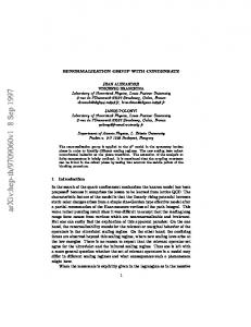
Figure 1: Example of eye diagram which contribute to K → ππ decay in the ∆I = 1/2 channel.
If chiral symmetry was exact, the operators of different chirality would not mix under renormalization, and in the basis described above the renormalization matrix would take the block diagonal form: ∆s=1 Z11 ∆s=1 Z ∆s=1 Z ∆s=1 Z ∆s=1 Z22 23 25 26 ∆s=1 ∆s=1 ∆s=1 ∆s=1 Z32 Z33 Z35 Z36 ∆s=1 ∆s=1 ∆s=1 ∆s=1 ∆s=1 . Z = (2.2) Z52 Z53 Z55 Z56 ∆s=1 ∆s=1 ∆s=1 ∆s=1 Z62 Z63 Z65 Z66 ∆s=1 ∆s=1 Z77 Z78 ∆s=1 Z ∆s=1 Z87 88 Furthermore, since ispospin is an exact symmetry in the chiral limit, for the (27,1) and (8,8) operators, it is enough to consider only the ∆I = 3/2 parts. This is numerically advantageous because the “eye diagram” (see fig. 1) which are difficult to compute can only contribute to ∆I = 1/2 processes.
3. Neutral kaon mixing In the standard model, neutral kaon mixing is dominated by box diagrams like the one shown 0 0 ∆s=2 in figure 2. The non-perturbative contributions are given by hK |O∆s=2 VV+AA |K i, where OVV+AA is the parity conserving part of (sγµL d)(sγµL d). Beyond the standard model, other operators contribute and they are usually given in the so-called SUSY basis O∆s=2 = (sα γµ (1 − γ5 )dα ) (sβ γµ (1 − γ5 )dβ ) , 1
(3.1)
O∆s=2 2 O∆s=2 3 O∆s=2 4 O∆s=2 5
= (sα (1 − γ5 )dα ) (sβ (1 − γ5 )dβ ) ,
(3.2)
= (sα (1 − γ5 )dβ ) (sβ (1 − γ5 )dα ) ,
(3.3)
= (sα (1 − γ5 )dα ) (sβ (1 + γ5 )dβ ) ,
(3.4)
= (sα (1 − γ5 )dβ ) (sβ (1 + γ5 )dα ) .
(3.5)
3
Nicolas Garron
W
s
d
t
t
W
d
s
Figure 2: Example of box diagram contributing to K − K mixing in the Standard model.
In this basis O∆s=2 is the standard model operator and O∆s=2 , i > 1 are the BSM ones. In the SU(3) i 1 ∆s=2 to the ∆I = 3/2 components of the and O flavor limit, It is straightforward to relate O∆s=2 4 5 electroweak penguins Q07 and Q08 , which transform under (8, 8). As one can find out from their transform under (6, 6) 1 . Thus, if chiral and O∆s=2 flavor structures, the remaining operators O∆s=2 3 2 symmetry is respected, O∆s=2 renormalizes multiplicatively, O∆s=2 and O∆s=2 mix together, and so 1 2 3 ∆s=2 ∆s=2 do O4 and O5 . To simplify the numerical implementation we work in the following basis: Q∆s=2 = (sα γµ dα )(sβ γµ dβ ) + (sα γµ γ5 dα )(sβ γµ γ5 dβ ) , 1
renormalizes multiplicatively, Q∆s=2 mixes It follows from the above considerations that Q∆s=2 1 2 ∆s=2 ∆s=2 ∆s=2 with Q3 and Q4 mixes with Q5 . We denote the renormalization factors computed in this basis by Zi∆s=2 . Moreover, in the SU(3) flavor limit they are some relations between the renormaj lization factors of the ∆s = 2 operators (3.6)-(3.10) and those of the ∆s = 1 operators (2.1). For example O∆s=2 and Q01 have the same renormalization factor, and the two by two renormalization 1 ) in the following way matrix of (Q7 , Q8 ) is related to the one of (Q∆s=2 , Q∆s=2 3 2 ∆s=1 = − 1 Z ∆s=2 Z87 2 32 ∆s=1 = Z ∆s=2 Z33 88
∆s=1 = Z ∆s=2 Z77 22 ∆s=1 = −2Z ∆s=2 Z87 32 1 In the literature,
(3.14)
we sometimes find the notation VLL for O1 , SLL for the set (O2 , O3 ) and LR for the set (O4 , O5 ).
4
Nicolas Garron
4. Numerical implementation and preliminary results The numerical setup of this computation is the same as the one presented in details in two recent publications [1, 13]. We use n f = 2 + 1 flavors of domain wall fermion on a Iwasaki gauge action at two values of the lattice spacing a ∼ 0.086 fm and a ∼ 0.114 fm , corresponding to the lattice volumes 32 × 64 × 16 and 24 × 64 × 16, respectively. On each ensemble the strange sea quark mass is fixed, while several values of the light sea quark masses have been considered (the corresponding unitary pion mass varies in the range 290 − 420 MeV). In this work we consider only the light valence quark masses which have the same values as their corresponding sea quarks, and perform the chiral extrapolations linearly in the quark mass. This computation was done with 20 configurations, and 100 bootstrap samples. In addition to the standard RI-MOM scheme, we implement also a scheme with non-exceptional (and symmetric) kinematic, which exhibits a better infrared behavior 2 [14, 15]. We also employ momentum sources [16] in order to obtain small statistical errors despite the expensive cost of the quark discretization. Furthermore, we use twisted periodic boundary conditions, which allows us to change smoothly the magnitude of the momentum without changing its direction (and thus control the O(4) discretization effects) [17]. This setup has been used recently used for the computation of ZBK [1]. Here we generalize this computation to the operators relevant for neutral kaon mixing beyond the standard model, and to the ∆I = 3/2 part of K → ππ decay. As described in [18], the Z matrix is essentially the invert of Λi j = Pj {Oi }, where Oi is a four-quark operator which belong to the basis given in eqs (3.6)-(3.10). Pj projects onto the Dirac and color structure of the operator O j (and a given flavor structure which depends on the choice of external states). In figures 3 and 4 we show the normalized Green vertex function Λi j extrapolated to the chiral limit. The range of simulated momenta corresponds to 1.98 GeV ≤ p ≤ 3.29 GeV on the finest lattice and to 1.80 GeV ≤ p ≤ 2.64 GeV on the coarser one. As expected the use of the momentum sources give us access to a very high statistical precision: at a given momentum the statistical error is below the permille (∼ 10−4 for ZBK ). Thanks to the twisted boundary conditions, the Z factors are smooth functions of the momentum (no scatter coming from the O(4) discretization effects is visible). Finally the effect of the non-exceptional kinematic is clearly visible in figure 4. The matrix elements shown in these plots should be zero if chiral symmetry was exact. With the Domain-Wall fermions, this is true only in the limit Ls → ∞, so in practice one has to check whether the effects of chiral symmetry breaking can be seen within the numerical precision. For the non-perturbative renormalization, this can be complicated by the presence of some Goldstone poles, which can affect the vertex functions. These poles are suppressed by the use of a non-exceptional kinematic. We confirm here an effect already seen in [4], that the good properties of the Domain Wall action can be obscured by a poor choice of kinematic.
2 The
non-exceptional scheme implemented here is called SMOM(γµ , γµ ) in [1]
5
Nicolas Garron
2
2 2 Λ11/Λ AV 2 Λ22/Λ AV 2 Λ23/Λ AV 2 Λ32/Λ AV 2 Λ33/Λ AV 2 Λ44/Λ AV 2 Λ45/Λ AV 2 Λ54/Λ AV 2 Λ55/Λ AV
1.5
1
0.5
0
2 AV 2 Λ22/Λ AV 2 Λ23/Λ AV 2 Λ32/Λ AV 2 Λ33/Λ AV 2 Λ44/Λ AV 2 Λ45/Λ AV 2 Λ54/Λ AV 2 Λ55/Λ AV
Λ11/Λ 1.5
1
0.5
0
-0.5
-0.5 1
2
1.5 (ap)
1
2.5
2
1.5
2
(ap)
2.5
2
Figure 3: Physical Green vertex functions for the non exceptional kinematic (SMOM scheme), in the chiral limit. On the left panel we show the results for the 243 lattice (a ∼ 0.114 fm) and on the right for the 323 lattice (a ∼ 0.086 fm). The error bars are smaller than the symbols.
2
0
-2
-4
-6
2 AV 2 Λ13/Λ AV 2 Λ14/Λ AV 2 Λ15/Λ AV 2 Λ21/Λ AV 2 Λ24/Λ AV 2 Λ25/Λ AV 2 Λ31/Λ AV 2 Λ34/Λ AV 2 Λ35/Λ AV 2 Λ41/Λ AV 2 Λ42/Λ AV 2 Λ43/Λ AV 2 Λ51/Λ AV 2 Λ2.5 /Λ AV 52 2 Λ53/Λ AV
Λ12/Λ
4
1
2
1.5 (ap)
2
2 AV 2 Λ13/Λ AV 2 Λ14/Λ AV 2 Λ15/Λ AV 2 Λ21/Λ AV 2 Λ24/Λ AV 2 Λ25/Λ AV 2 Λ31/Λ AV 2 Λ34/Λ AV 2 Λ35/Λ AV 2 Λ41/Λ AV 2 Λ42/Λ AV 2 Λ43/Λ AV 2 Λ51/Λ AV 2 Λ2.5 /Λ AV 52 2 Λ53/Λ AV
Λ12/Λ 0.004
0.002
0
-0.002
-0.004
-0.006
-0.008
1
2
1.5 (ap)
2
Figure 4: Chiraly disallowed Green vertex functions on the finest lattice for the exceptional (left) and nonexceptional (right) kinematic. We see that for the exceptional kinematic some of these matrix elements are suppressed only at high momenta, while in the non exceptional case they are all zero within the statistical precision.
5. Conclusions and outlook By combining momentum source with twisted boundary conditions and non exceptional kinematic we can obtain the renormalization factors of kaon four-quark operators with a very good handle on the different kinds or errors: the statistical errors are tiny (below the permille), most of 6
Nicolas Garron
the unwanted infrared effects are suppressed and the usual scatter coming from the O(4) discretization errors is absent. Even with this precision, when a non-exceptional kinematic is implemented, the non-physical mixing of the four-quark operators is compatible with zero, thanks to the good chiral properties of the Domain Wall action. We are currently extending our computation to a larger physical volume discussed in [9], where the simulated pion mass is significantly smaller (down to 180 MeV). We plan to use the step scaling method introduced in[17] in order to enlarge the RomeSouthampton window. We have also started a computation of the eye diagrams, with the use of stochastic sources. We thank our RBC/UKQCD colleagues for many discussions and contributions to this work.
References [1] Y. Aoki et al., (2010), 1012.4178. [2] A. Donini et al., Phys. Lett. B470 (1999) 233, hep-lat/9910017. [3] R. Babich et al., Phys. Rev. D74 (2006) 073009, hep-lat/0605016. [4] RBC, J. Wennekers, PoS LATTICE2008 (2008) 269, 0810.1841. [5] ETM, P. Dimopoulos et al., (2010), 1012.3355. [6] Particle Data Group, K. Nakamura et al., J. Phys. G37 (2010) 075021. [7] S. Li and N.H. Christ, PoS LATTICE2008 (2008) 272, 0812.1368. [8] L. Lellouch and M. Lüscher, Commun. Math. Phys. 219 (2001) 31, hep-lat/0003023. [9] E.J. Goode and M. Lightman, PoS LATTICE2010 (2010) 313, 1101.2473. [10] J. Laiho and R.S. Van de Water, (2010), 1011.4524. [11] C.W. Bernard, Lectures given at TASI ’89, Boulder, CO, Jun 4-30, 1989. [12] RBC, T. Blum et al., Phys. Rev. D68 (2003) 114506, hep-lat/0110075. [13] RBC, Y. Aoki et al., (2010), 1011.0892. [14] Y. Aoki et al., Phys. Rev. D78 (2008) 054510, 0712.1061. [15] C. Sturm et al., Phys. Rev. D80 (2009) 014501, 0901.2599. [16] M. Gockeler et al., Nucl. Phys. B544 (1999) 699, hep-lat/9807044. [17] RBC-UKQCD, R. Arthur and P.A. Boyle, (2010), 1006.0422. [18] G. Martinelli et al., Nucl. Phys. B445 (1995) 81, hep-lat/9411010.