Non Pre-emptive Scheduling of Messages on ... - Semantic Scholar

Submission to the 12th Euromicro Conference on Real-Time Systems Royal Institute of Technology, Stockholm, Sweden, June 19th - 21st, 2000

Non Pre-emptive Scheduling of Messages on SMTV Token-Passing Networks Eduardo Tovar

Francisco Vasques

Department of Computer Engineering, ISEP, Polytechnic Institute of Porto Rua São Tomé, 4200-072 Porto, Portugal E-mail: [email protected]; Fax: +351.22.8321159

Department of Mechanical Engineering, FEUP, University of Porto Rua Bragas, 4050-123 Porto, Portugal E-mail: [email protected]

Abstract Fieldbus communication networks aim to interconnect sensors, actuators and controllers within distributed computer-controlled systems. Therefore, they constitute the foundation upon which real-time applications are to be implemented. A specific class of fieldbus communication networks is based on a simplified version of tokenpassing protocols, where each station may transfer, at most, one Single Message per Token Visit (SMTV). In this paper, we establish an analogy between non pre-emptive task scheduling in single processors and scheduling of messages on SMTV token-passing networks. Moreover, we clearly show that concepts such as blocking and interference in non pre-emptive task scheduling have their counterparts in the scheduling of messages on SMTV token-passing networks. Based on this task/message scheduling analogy, we provide prerun-time schedulability conditions for supporting real-time messages with SMTV token-passing networks. We provide both utilisation-based and response time tests to perform the pre-run-time schedulability analysis of realtime messages on SMTV token-passing networks, considering RM/DM and EDF priority assignment schemes. Neither this paper nor any version close to it has been or is being offered elsewhere for publication. All necessarily clearances have been obtained for the publication of this paper. If accepted, the paper will be made available in camera ready forms by March 15th, 2000, and it will be personally presented at RTS'00 by one of the authors. The presenting author(s) will pre-register for RTS'00 before the due dates of the camera-ready paper.

1. Introduction Local area networks (LANs) are becoming increasingly popular in industrial computer-controlled systems. LANs allow field devices like sensors, actuators and controllers to be interconnected at low cost, using less wiring and requiring less maintenance than point-to-point connections. Besides the economic aspects, the use of LANs in industrial computer-controlled systems is also reinforced by the increasing decentralisation of control and measurement tasks, as well as by the increasing use of intelligent microprocessor-controlled devices. Broadcast LANs aimed at the interconnection of sensors, actuators and controllers are commonly known as fieldbus networks. Fieldbus networks are widely used as the communication support for distributed computer-controlled systems (DCCS), in applications ranging from process control to discrete manufacturing. Usually, DCCS impose real-time requirements; that is, traffic must be sent and received within a bounded interval, otherwise a timing fault is said to occur. This motivates the use of communication networks within which the medium access control (MAC) protocol is able to schedule messages according to their real-time requirements. One of the MAC protocols used in widely accepted fieldbus networks is based on a simplified version of the token-passing protocol. In these fieldbus networks (PROFIBUS and P-NET are just two examples) there are typically two types of network nodes: masters and slaves. This MAC protocol is based on a token-passing procedure used by master stations to grant the bus access to each other, and a master-slave procedure used by master stations to communicate with slave stations. Each time a master receives the token, it will be able to perform, at most, one message cycle. We denote this type of networks as Single Message per Token Visit (SMTV) token-passing networks. -1-

A message cycle consists of a master's action frame (request or send/request frame) and the associated responder's acknowledgement or response frame. We assume that responses from slaves are immediate, with a bounded turnaround time. At each master node, requests generated at the application process (AP) level are placed in the master's outgoing queue. At each token arrival, the highest priority message cycle will be processed. We assume the following message stream model:

Sik = (Cik , Ti k , Dik )

(1)

Sik defines a message stream i in master k (k = 1, ..., n). A message stream is a temporal sequence of message cycles concerning, for instance, the remote reading of a specific process variable. Cik is the longest message cycle duration of stream Sik. This duration includes both the longest request and response transmission times, and also the worst-case slave's turnaround time. Tik is the periodicity of stream Sik requests. In order to have a subsequent timing analysis independent from the model of the tasks at the application process level, we assume that this periodicity is the minimum interval between two consecutive arrivals of Sik requests to the outgoing queue. Finally, Dik is the relative deadline of a message cycle; that is, the maximum admissible time interval between the instant when the message request is placed in the outgoing queue and the instant at which the related response is completely received at the master's incoming queue. Finally, nsk denotes the number of message streams associated with a master k. In our model, the relative deadline of a message can be equal or smaller than its period (Dik ≤ Tik). Thus, if in the outgoing queue there are two message requests from the same message stream, this means that a deadline for the first of the requests was missed. Therefore, the maximum number of pending requests in the outgoing queue will be nsk. We denote the worst-case response time of a message stream Sik as Rik. This time is measured starting at the instant when the request is placed in the outgoing queue, until the instant when the response is completely received at the incoming queue. Basically, this time span is made up of two components. One concerns the time spent by the request in the outgoing queue, until gaining access to the bus (queuing delay). The other concerns the time needed to process the message cycle, that is, to send the request and receive the related response (transmission delay). Thus,

Rik = Qik + Cik

(2)

where Qik is the worst-case queuing delay of a message request from Sik. Analysis for the worst-case response time can be performed if the worst-case token rotation time is assumed for all token cycles. Assume also that CM is the maximum transmission duration of a message cycle. If a master uses the token to perform a message cycle, we can define the token holding time as:

H = ρ + CM + τ

(3)

where the symbol τ denotes the time to pass the token after a message cycle has been performed and the symbol ρ denotes the master’s worst-case reaction time. As the token rotation time is the time interval between two consecutive token visits, the worst-case token rotation time, denoted as V, is:

V = n× H

-2-

(4)

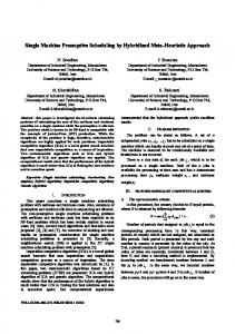
Considering priority-based dispatching mechanisms, the worst-case response time for a message request occurs when the request is placed in the master's queue just after the token arrival, hence not being able to be processed in that token visit. If there were any other message request pending before the token arrival, then the token would have been used to transmit that message; otherwise, the master would not use the token at all. Therefore, the worst-case response time of a message stream Sik will be:

Rik = Qik + Cik = V + Φ × V + Cik

(5)

where the first term V denotes the message blocking, and the symbol Φ denotes the number of higherpriority messages (interference) that can be scheduled ahead of a message from Sik. Fig. 1 illustrates the case where Φ equals 0 (highest priority message cycle S11). highest priority request from master 1 released marginally after the token arrival

a lower priority message induces a priority inversion with length V

highest priority requests processed here

req(S11)

res(S11)

Bus

Master holding the token

1

3

2 τ

H

1

2

ρ

V

CM

Figure 1

The remainder of this paper is organised as follows. In Section 2 we survey some relevant results for the priority-based schedulability analysis of real-time tasks, both for fixed and dynamic priority assignment schemes. We give emphasis to the worst-case response time analysis in non pre-emptive contexts, since that analysis is of paramount importance to the message schedulability analysis in SMTV token-passing communication networks. In Section 3 we discuss the analogy between task scheduling in a single processor environment and message scheduling in SMTV token-passing networks. Based on this task/message scheduling analogy we provide utilisation-based tests and response time tests, in Section 4 and Section 5, respectively, for SMTV token-passing networks. In both cases, RM/DM and EDF priority assignment schemes are considered. Finally, in Section 6, some conclusions are drawn.

2. Schedulability Analysis of Tasks in Single Processor Systems Real-time computing systems with tasks dispatched according to a priority-based policy (we consider only RM/DM or EDF), must be tested a-priori in order to check if, during run time, no deadline will be missed. This feasibility test is called the pre-run-time schedulability analysis of the task set. There are mainly two types of analytical methods to perform pre-run-time schedulability analysis. One is based on the analysis of the processor utilisation. The other is based on the response time analysis for each individual task. In [1], the authors demonstrated that by considering only the processor utilisation, a test for the pre-run-time schedulability analysis could be obtained. Contrarily, a response time test must -3-

be performed in two stages. First, an analytical approach is used to predict the worst-case response time of each task. The values obtained are then compared, trivially, with the relative deadlines of the tasks. The utilisation-based tests have a major advantage: it is a simple computation procedure, which is applied to the overall task set. By this reason, they are very useful for implementing schedulers that check the schedulability online. However, utilisation-based tests have also important drawbacks, when compared with their response-time counterparts. They do not give any indication of the actual response times of the tasks. More importantly, and apart from particular task sets, they constitute sufficient but not necessary conditions. This means that if the task set passes the test, the schedule will meet all deadlines, but if it fails the test, the schedule may or may not fail at run-time (hence, there is a certain level of pessimism). It is also worth mentioning that the utilisation-based tests cannot be used for more complicated task models [2]. 2.1. Schedulability Tests: Case of the Fixed Priority Assignment 2.1.1. Basic Utilisation-Based Test For the RM priority assignment, Liu and Layland introduced an utilisation-based sufficient test: N

Ci

∑T i =1

(

)

≤ N × 21 N − 1

(6)

i

This utilisation-based test is valid for periodic independent tasks, with relative deadlines equal to the period, and for pre-emptive systems. In [3], the authors provide an exact analysis:

 i   l × Tk   Tj × min ∑ U j ×   ≤ 1, ∀i, 1≤i≤n ( k ,l )∈Ri j =1  l × Tk  T j     

(7)

where Ri = {(k,l)} with 1 ≤ k ≤ i and l = 1, ..., Ti/Tk. It is clear that inequality (7) is not an easy to use test, hence loosing one of the advantages inherent to the more basic formulations: its simplicity. 2.1.2. Extended Utilisation-Based Tests In [4], the authors update the utilisation-based test (6) to include blocking periods, during which higherpriority tasks are blocked by lower-priority ones, to solve the problem of non-independence of tasks:

 i Ci  ∑  i =1 Ti

 Bi  + ≤ i × 21 i −1 , ∀i , 1≤i≤ N  Ti

(

)

(8)

where Bi is the maximum blocking a task i can suffer. This analysis can be extended to a non pre-emptive context, since in this case a higher-priority task can also be "blocked" by a lower-priority task. Assuming that the tasks are completely independent, the maximum blocking time a task can suffer is given by:

if Pi = min {Pj }  Bi = 0, j =1,.., N   {C j }, if Pi ≠ jmin {Pj }  Bi = max =1,.., N j∈lp (i )

-4-

(9)

where lp(i) denotes the set of lower-priority tasks (than task i). Therefore, inequality (8) can be used as an utilisation-based test for a set of non pre-emptable independent tasks, with the blocking for each task as given by (9). Moreover, accepting an increased level of pessimism, inequality (8) can be simplified to:

 N Ci  ∑  i =1 Ti

 B   + max  i  ≤ i × 21 N −1  i, 1≤i ≤ N  Ti 

(

)

(10)

Note that if all tasks have the same computation time, (10) considers that each task may be blocked at the rate of the highest-priority task. 2.1.3. Response Time Tests for the Pre-emptive Context In [5] the authors proved that the worst-case response time Ri of a task i is found when all tasks are synchronously released (critical instant) at their maximum rate. Ri is defined as:

Ri = I i + Ci

(11)

where Ii is the maximum interference that task i can experience from higher-priority tasks in any interval [t, t + Ri). Without loss of generality, it can be assumed that all processes are released at time instant 0. Consider a task j with higher-priority than task i. Within the interval [0, Ri), it will be released Ri/Tj times. Therefore, each release of task j will impose an interference Cj. The worst-case response time Ri of a task τi is then:

Ri =

R    i  × C  + C ∑ j i  j∈hp(i )  T j   

(12)

where hp(i) denotes the set of higher-priority tasks (than task i). Equation (12) embodies a mutual dependence, since Ri appears in both sides of the equation. The easiest way to solve such equation is to form a recurrence relationship [6]:

Wi m +1 =

 W m    i  ×C  + C ∑ j  i j∈hp(i )  Tj   

(13)

The recursion ends when Wim+1 = Wim = Ri and can be solved by successive iterations starting from Wi0 = Ci. Indeed, it is easy to show that Wim is non-decreasing. Consequently, the series either converges or exceeds Ti (case of RM) or Di (case of DM). If the series exceeds Ti (or Di), the task τi is not schedulable. 2.1.4. Response Time Tests for the non Pre-emptive Context In [6] the authors updated the analysis of [5] to include blocking factors introduced by periods of non pre-emption, due to the non-independence of the tasks. The worst-case response time is updated to:

Ri = Bi +

R 



∑( )  T  × C  + C i

j∈hp i



j



j



i

(14)

which may also be solved using a similar recurrence relationship. Bi is also as given by equation (9). Some care must be taken using equation (14) for the evaluation of the worst-case response time of non pre-emptable independent tasks. In the case of pre-emptable tasks, with equation (12) we are finding the processor's level-i busy period preceding the completion of task i; that is, the time during which task i

-5-

and all other tasks with a priority level higher than the priority level of task i still have processing remaining. For the case of non pre-emptive tasks, there is a slight difference, since for the evaluation of the processor's level-i busy period we cannot include task i itself; that is, we must seek the time instant preceding the execution start time of task i. Therefore, equation (11) can be used to evaluate the task's response time of a task set in a non preemptable context and independent tasks, where the interference is:

I i = Bi +

  Ii    C ×   ∑ j   T j∈hp(i )  j   

(15)

Note also that a re-definition for the critical instant must be made. The maximum interference occurs when task i and all other higher-priority tasks are synchronously released just after the release of the longest lower-priority task (than task i). 2.2.

Schedulability Tests: Case of the Dynamic Priority Assignment

2.2.1. Basic Utilisation-Based Test For the EDF priority assignment, Liu and Layland also introduced an utilisation-based pre-run-time schedulability test (16), valid for non pre-emptive, independent and periodic tasks, for which the relativedeadline is equal to the period. N

Ci

∑T i =1

≤1

(16)

i

Inequality (16) can be easily updated to include blocking periods due to the non-independence of the tasks. In [7], the author updated inequality (16) to:

 i Ci  ∑  i =1 Ti

 Bi  + ≤ 1, ∀i, 1≤i≤ N  Ti

(17)

where Bi is the maximum blocking a task i can suffer, considering the stack resource protocol (SRP). The key idea behind the SRP is that when a job needs a resource which is not available, it is blocked at the time it attempts to pre-empt, rather than later. This makes inequality (17) valid for sets of non preemptable tasks, dispatched according to the EDF scheme. Similarly to the updating of (8) to (10), (17) can be updated to a simpler (but more pessimistic) test:

 N Ci  ∑  i =1 Ti where Bi is defined as:

 B   + max  i  ≤ 1  i, 1≤i≤ N  Ti 

Bi = max{C j } j ≠i

(18)

(19)

Another relevant result from [7] is that (17) can also be extended to task sets with relative deadlines smaller than periods:

 i Ci  ∑  i =1 Di

 Bi  + ≤ 1, ∀i , 1≤i≤ N  Di -6-

(20)

As a corollary, inequality (16) can be extended for task sets with Di ≤ Ti: N

Ci

∑D i =1

≤1

(21)

i

These simple utilisation-based tests ((18) and (20)) are however quite pessimistic. Less pessimistic utilisation-based tests will now be addressed in Sections 2.2.2 and 2.2.3, for pre-emptive and non preemptive tasks, respectively. Later, in Sections 2.2.4 and 2.2.5, recent results on response time analysis will be addressed, for pre-emptive and non pre-emptive tasks, respectively. 2.2.2. Extended Utilisation-Based Tests for the Pre-emptive Context In [8] the author extends the results of Liu and Layland in order to consider sporadic tasks, where inequality (16) is updated to: +

 t − Di  ∑   × C i ≤ t , ∀ t ≥0 i =1  Ti  N

(22)

with x+ = 0 if x < 0. This formulation has advantages over (20), in the sense that it turns out to be a necessary and sufficient condition. Inequality (22) can not be classified as a simple test when compared to (20). It has also an additional problem, since it must be checked over an infinite continuous time interval [0, ∞). A simplification to the schedulability test can be made considering that the right side of inequality (22) does only change at k×Ti+Di time instants, and thus the inequality does only need to be checked for these time instants. Different authors have addressed the problem of finding an upper limit for t. It is possible to prove that if the total utilisation of the processor is ≤ 1 (condition (16)), it exists a point tmax, such that ∑i=1,..,n((t – Di)/Ti+ × Ci) ≤ t always hold, ∀t ≥ t . Consequentely, inequality (22) can be max

re-written as follows: +

 t − Di  N   U {Di + k × Ti , k ∈ ℵ} ∩ [0, t max ) C t , , with S × ≤ ∀ = ∑ i t∈S   i =1  Ti  i =1   N

(23)

In [9] the authors demonstrated that tmax could be given by (U/(1-U))×maxi=1,...,.N{(Ti-Di)}, where U represents the overall processor's utilisation (∑i=1,...,.N (Ci/Ti)). This result was further improved in [10], where the upper bound for t is defined as tmax=((∑i=1,...,.N (1-Di/Ti)×Ci)/(1-U). Although this last formulation gives a smaller value for tmax, it still suffers from the same disadvantage: as the overall utilisation approaches 1, its value becomes very large. Another approach is considered in [10] and [11], where the authors demonstrate that tmax = L (synchronous processor's busy period). The synchronous processor's busy period is defined as the time interval from the critical instant up to the first instant when there are no more pending tasks in the system: N L L = ∑   × Ci i =1  Ti 

Equation (24) may be solved by recurrence, starting with L0 = ∑i=1,..,NCi.

-7-

(24)

2.2.3. Extended Utilisation-Based Tests for the non Pre-emptive Context For the non pre-emptive context, a similar test was presented in [8] and [12]: +

 t − Di  {C j }≤ t , ∀ t ≥ Dmin , with Dmin = jmin {D j } ∑   × C i + jmax =1,..., N =1,...,N i =1  Ti  N

(25)

Comparing to the test for the pre-emptive context (22), the inclusion of the blocking factor is intuitive (see Section 2.2.1.). However, in [13] the authors discuss the pessimism inherent to the inequality (25). The main argument is that in this inequality it is considered that the cost of possible priority inversions is always initiated by the longest task and, moreover, it is effective during the entire interval under analysis. To reduce this level of pessimism, it is suggested the following modification: +

 t − Di  {C j }≤ t , ∀ t∈S , with jmax {C j }= 0 if ∃/ j : D j > t ∑   × C i + jmax =1,..., N =1,..., N i =1  Ti  D j >t D j >t N

(26)

That is, the blocking factor is only included if its deadline occurs after t. 2.2.4. Response Time Tests for the Pre-emptive Context The worst-case response time analysis for pre-emptive EDF scheduling was first introduced in [14]. In his work, Spuri demonstrated that the worst-case response time of a task i is found in the processor's deadline-i busy period (analogous to the processor's level-i busy period in the case of fixed priorities). However, the longest processor's deadline-i busy period may occur when all tasks but task i (contrarily to the case of fixed priority assignment) are synchronously released and at their maximum rate. This means that, in order to find the worst-case response time of task i, we need to examine multiple scenarios within which, while task i has an instance released at time a, all other tasks are synchronously released at time t = 0. Thus, given a value of a, the response of an instance of task i is:

Ri (a ) = max{Ci , Li (a ) − a}

(27)

where Li(a) is the length of the deadline-i busy period, which starts at time instant t = 0. Li(a) can be evaluated by the following iterative computation:

Li (a ) =

     min  Li (a ) , 1 +  a + Di − D j   × C  + 1 +  a   × C   ∑ j     Ti   i Tj  T j  j ≠i       D j ≤ a + Di 

(28)

Equation (28) can be solved by recurrence, starting with Li0(a) = 0. Obviously, in equation (28), the computational load only considers tasks that have deadlines earlier than Di. Finally, in the general case, the worst-case response time for a given task i is:

Ri = max{Ri (a )} a ≥0

(29)

The remaining problem is how to determine the values of a. Looking to the right-hand side of equation (28), we can easily understand that its value only changes at k × Tj + Dj – Di steps.

-8-

a ∈ U {k × T j + D j − Di , k ∈ℵ0 }∩ [0, L[ N

j =1

(30)

with L as given by equation (24). 2.2.5. Response Time Tests for the non Pre-emptive Context The worst-case response time analysis for the non pre-emptive EDF scheduling was introduced in [13]. The main difference from the analysis for the pre-emptive case is that a task instance with a later absolute deadline can cause a priority inversion. Thus, and similarly to the fixed priority case (Section 2.2.4), instead of analysing the deadline-i busy period preceding the completion time of task i, we must analyse the busy period preceding the execution start time of the task’s instance. Consequently, the response time of the τi ‘s instance released at time a is:

Ri (a ) = max{C i , Li (a ) + C i − a}

(31)

where Li(a) is now the length of the busy period (preceding execution). Thus, Ri(a) can be evaluated by means of the following iterative computation:

Li (a ) = max {C j }+ D j > a + Di

     min 1 +  Li (a ) , 1 +  a + Di − D j   × C  +  a  × C   j    Ti  i T j  Tj j ≠i            D j ≤ a + Di 

∑

(32)

3. From Task to Message Scheduling in SMTV Networks: Analogies In this section we discuss the analogy between task scheduling in a single processor environment and message scheduling in SMTV token-passing networks. This analogy will later enable the formulation of feasibility tests for the pre-run-time schedulability analysis of message stream sets in SMTV tokenpassing networks. In the schedulability analysis of tasks in the non pre-emptive context, the concept of processor's busy period denotes the time interval within which the processor is not idle (see Section 2.1.4). Consider the following task set example (D=T): Table 1 Task

Computation Time (C)

Period (T)

A B C D

10 10 10 10

60 80 100 100

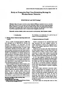
Assuming a RM priority assignment policy in a non pre-emptive context, Fig. 2 illustrates a time-line considering that the first instance of task D (lower-priority task) is released marginally after time instant 0, and before all other instances of higher-priority tasks. Note that the blocking of a task in a non preemptive context is equal to the maximum execution length of a lower-priority task (see equation (9)). Consider now the following message stream set example (where D=T) to be scheduled in a SMTV tokenpassing network:

-9-

Table 2 Message

Message Cycle Length (C)

Period (T)

A B C D

2 2 2 2

60 80 100 100

This case will be shown to be loosely equivalent to the previous task scheduling example, when the token cycle time is equal to the tasks' execution time (V = Ctask). Maximum blocking for a higher priority task (as all Cs are equal)

When this request appears, there is no pending task

Time utilisation of the shared resource (processor) by a task

Task D

Task C

Task B

Task A

10

20

30

40

50

60

70

80

90

100 110 120 130 140 150 160 170 180

processor busy period release of task

Figure 2

Consider now Fig. 3, which illustrates the time-line for a message scheduling on a SMTV token-passing network, considering a messages' release pattern (arrival of requests to the outgoing queue) similar to the previous tasks' release pattern. It is clear that the message blocking time is equal to the token cycle time. However, this blocking term is independent of the priority ordering of message transfers. Therefore, the blocking problem in the task scheduling theory can only be considered to be loosely equivalent to the blocking problem in SMTV token-passing networks, since the priority ordering property is not preserved. This request appears just after the token arrival, hence it is not able to be processed in this token visit

Time utilisation of the shared resource (token/network) by a message cycle, as seen by the local station

Maximum blocking for any-priority message cycle

Message D

Message C

Message B

Message A

10

20

30

40

50

60

70

80

100 110 120 130 140 150 160 170 180 V

token busy period

Arrival of the request to the queue

90

Instant of token arrival

Figure 3

-10-

It is also clear that tests available for the schedulability analysis of non pre-emptable tasks in single processor systems can be adapted to the message scheduling in SMTV token-passing networks, considering that the blocking term is equal to the token cycle time, independently of the message priority. Therefore, the computation time of a task can be considered equivalent to the token cycle time, since in a SMTV token-passing network the shared resource (network access/token) is available once in every V interval. This means that the contribution of each higher-priority message cycle to the overall queuing delay of a lower-priority message cycle is always equal to V. Finally, in Table 3 we summarise the analogies between task scheduling in non pre-emptive single processor environments and message scheduling in SMTV token-passing networks. Table 3 Task Scheduling Maximum blocking (except for the lowest priority task/message)

Bi = max {C j }

Message Scheduling

∀j∈lp (i )

V

Maximum blocking (lowest priority task/message)

0

V

Resource usage time for the higher-priority tasks/messages

Cj

V

Resource usage time for the task/message itself

Ci

Ci

Considering these analogies between task scheduling and message scheduling, a set of (token) utilisationbased and response time tests can be developed for the schedulability analysis of SMTV token-passing networks. In the following sections we present both types of tests.

4. (Token) Utilisation-Based Tests In this section, we derive (token) utilisation-based schedulability tests for both fixed and dynamic priority assignment schemes. Such schedulability tests, which can be quite pessimistic, provide an easy tool to evaluate the schedulability of the overall message set with a reduced complexity. 4.1.

Case of Rate Monotonic Priority Assignment

Considering the analogies to the blocking and tasks' computation time drawn in the previous section, the schedulability test (10) for the RM dispatched tasks can be adapted to encompass the characteristics of the SMTV token-passing protocol, as follows:

 ns V ∑ k  i= T  1 i k

 1   V   + max  k  ≤ ns k ×  2 ns k − 1, ∀ k  1≤ i ≤ n T    i    

(33)

As the worst-case token cycle time (V) is constant, equation (33) can be re-written as:

 ns 1 V ×  ∑ k  i =1 Ti k

 1 +  min T k i 

  ns1k  k  2 − 1 , ∀ k ≤ ns ×      

{ }

(34)

Note that, as we are considering SMTV token-passing networks, the interference from other masters is only reflected on the evaluation of the V parameter.

-11-

Consider the following example, which highlights the use of the proposed schedulability test (34): Table 4 Stream

Period

S1k

5

S2k S3k S4k

7 8 12

Considering that the worst-case token rotation time is V = 1, it follows that the schedulability test is:  4 1 1 ×  ∑ k  i =1 Ti

  + 

  1 1 1 1 1 1 1 + = 0.75 ≤ 0.76  ≤ 4 ×  2 4 − 1 ⇔ + + + 5  5 7 8 12 5  

Therefore the message stream set of Table 4 is schedulable by the RM algorithm in a SMTV tokenpassing network. In Fig. 4, we present a possible time-line for the message scheduling, assuming that all messages are requested just after the first token arrival. In this way, we represent a blocking term at the beginning of the time-line.

S1k Requests at the AP level

S2k S3k S4k

1

2

3

4

5

6

7

8

9

10

11

12

13

14

15

16

17

...

Token arrivals

Message cycle processed

low

Priority queue (RM) hi

S1k

S2k

S3k

S4k

Figure 4

This example highlights the pessimism associated to the utilisation-based tests, since, although the schedulability test is just marginally true, none of the message cycles is scheduled close to its deadline. 4.2.

Case of Earliest Deadline First Priority Assignment

Considering again the analogies to the blocking and tasks' computation time drawn in Section 3, the schedulability test (18) for the EDF dispatched tasks can also be adapted to encompass the characteristics of the SMTV token-passing protocols, as follows:

 ns k 1 V ×  ∑ k  i =1 Ti 

 1 +  min T k  1≤ i ≤ n i

  ≤ 1, ∀ k  

{ }

(35)

Consider now the following example, where periods are considered to be marginally smaller than multiples of the worst-case token cycle time (V = 1): -12-

Table 5 Stream

Period

S1k S2k

45

S3k

6

k

8

S4

-

The application of the schedulability test (35) to this message stream set is:  4 1 1 ×  ∑ k  i =1 Ti

  + 

1 1 1 1 1 1  ≤ 1 ⇔  + + + +  ≤ 1 ⇔ 0.99 ≤ 1 TRUE 4  4 5 6 8 4

Hence, this message stream set is schedulable considering the EDF priority assignment scheme, while with the RM assignment scheme would not pass the schedulability test (34): 0.99 ≤ 0.76 is FALSE.

5. Response Time Tests In this section we derive response time schedulability tests for both fixed and dynamic priority assignment schemes. Such schedulability tests, compared to the (token) utilisation-based tests are more complex, but also much less pessimistic, as it will be shown in this section. This is an expected result, as response time tests for task scheduling are sufficient and necessary conditions, while the utilisation-based tests are generally only sufficient conditions (refer to Section 2). It is also important to note that for the case of Dik < Tik there are no simple utilisation-based tests for the case of fixed priorities. 5.1.

Response Time Tests: Fixed Priority Assignment

Based on the analogies between task scheduling and message scheduling on SMTV token-passing networks, the worst-case response time analysis for the non pre-emptive context (refer to Section 2.1.4) can be adapted to encompass the characteristics of the SMTV token-passing protocols. The worst-case message response is defined in equation (2), where Qik is:

  Qik    Qik   Q = V + ∑  k  ×V = V × 1 + ∑  k    ∀ ( ) Tj  ∀ j∈hp ( i )  T j  j∈hp i    k i

(36)

Note that this queuing delay is the equivalent to the task's interference in a non pre-emptive context (15). Considering again the message stream set example presented in Table 5, the worst-case response time for each message stream will be as shown in Table 6 (assuming Cik = 0.2, ∀i). Table 6 Stream

Response

S1k S2k S3k S4k

1.2 2.2 3.2 7.2

Considering the message stream S4k, the iterations for evaluating its queuing delay are as follows: Q 4k

(0 )

(1)  0  0 0  1  1  1  = 1 +  −  +  −  +  −  = 1; Q 4k = 1 +  −  +  −  +  −  = 4  4  5  6  4  5  6 

-13-

Q 4k Q 4k

(2 )

(4 )

(3 )  4 4  4 5  5 5 = 1 +  −  +  −  +  −  = 5; Q 4k = 1 +  −  +  −  +  −  = 6 4  5  6   4  5  6  (5 )  6  6 6  7  7 7  = 1 +  −  +  −  +  −  = 7; Q 4k = 1 +  −  +  −  +  −  = 7 4  5  6  4  5  6 

and iterations stop, since Q4k(5) = Q4k(4) = 7. Therefore, from equation (2) R4k = 7 + 0.2 = 7.2, which is smaller than its relative deadline (its period), and thus, the message stream set is RM schedulable. Considering the same message stream set, the (token) utilisation-based test (34) gives 0.99 ≤ 0.76, which is equivalent to state that this message stream set may or not be schedulable. Therefore, it turns out that the response time test is much less pessimistic than the (token) utilisation-based test. The time-line presented in Fig. 5 illustrates the above results.

S1k S2k

Requests at the AP level

S3k S4k

1

2

3

4

5

6

7

8

9

10

11

12

13

14

15

16

17

...

Token arrivals

Message cycle processed

low

Priority queue (RM) hi

S1k

S2k

S3k

S4k

Figure 5

5.2.

Response Time Tests: Dynamic Priority Assignment

Based on the analogies between task scheduling and message scheduling on SMTV token-passing networks, the worst-case response time analysis for the non pre-emptive context (refer to Section 2.2.5) can also be adapted to encompass the characteristics of the SMTV token-passing protocols. The worst-case message response time is, obviously, given by equation (2). However, a major difference exists for the definition of the queuing delay, which for the EDF case must be defined as:

  k k k         − D D Q   Qik = V × 1 + ∑ min 1 +  ik  , 1 +  i k j    j ≠i   T j   T j     k k D ≤ D j i  

(37)

that is, a message request concerning stream Sik will be delayed by all message requests of other streams having earlier or equal absolute deadlines than the absolute deadline for Sik (absolute deadlines are the difference between the relative deadline, Dik, and the beginning of the evaluation interval - assumed at time instant 0). Note that while ∑(1 +  Qik / Tjk  ) requests having relative deadlines smaller or equal to

-14-

Dik can be placed in the AP queue, from those requests, only a maximum of 1 +  (Dik - Djk)/ Tjk  will have absolute deadlines earlier than Dik. We illustrate this effect with the following example. Table 7 Stream

Period

S1k S2k S3k S4k

4567-

If we consider the synchronous release pattern for message streams (Table 7), a time-line for the EDF schedule may be as illustrated in Fig. 6.

S1k Requests at the AP level

S2k S3k S4k

1

2

3

4

5

6

7

8

9

10

11

12

13

14

15

16

17

...

Token arrivals

Message cycle processed

low

Priority queue (EDF) hi

S1k

S2k

S3k

S4k

Figure 6

As it can be seen from Fig. 6, there is a request for S1k arriving to the queue before the processing of the first request for S4k. However, as that request for S1k has an absolute deadline which is later than the absolute deadline for S4k, it will be processed only after the request for S4k. This behaviour of the EDF scheduler is effectively translated by equation (37), as can be seen by the following successive iterations (V = 1):   0   7 − − 4−    0   7 − − 5−  1 , 1 + + + = 1 + min 1 +  −  , 1 +      +  − −  −  5    5   5   4   0   7 − − 4−  + 1 +  −  , 1 +    = 1 + min {1, 1} + min {1, 1} + min {1, 1} = 4 −  6   6    4   7 − − 4−    4   7 − − 5−  (1) 1 , 1 Q 4k = 1 + min 1 +  −  , 1 +  + + +      + − −  −  5   5   5   4  − −   4  7 − 4  + 1 +  −  , 1 +    = 1 + min {2, 1} + min {1, 1} + min {1, 1} = 4 −  6   6  Q 4k

(0 )

and iterations stop, as Q4k(1) = Q4k(0) = 4. The maximum queuing delay for a request of stream S4k, considering that the streams have a synchronous release pattern, is thus as shown in Fig. 6.

-15-

Note however that the worst-case response time for EDF dispatched messages is not necessarily found with a synchronous release pattern (refer to Sections 2.2.4 and 2.2.5). Therefore, equation (37) must be updated to:

      Q k (a )   a + Dik − D kj     a   i  Q (a ) = B (a ) + V ×  ∑ min 1 +  k , 1 +   +  k   T jk   T j   k j ≠i k       Ti     D j ≤a + Di k i

k i

(38)

where Bik is defined as follows:

V , a = 0 Bik (a ) =  k k V , a ≠ 0 ∧ ∃ j : D j > a + Di

(39)

Note that while with the RM/DM approach (Section 5.1) the blocking term is V and effective for all the message streams, with the EDF approach, we must only consider (if a ≠ 0) a blocking if it exists a message stream Sjk (j ≠ i) with an absolute deadline later than the relative deadline of the instance of Sik released at time instant a. A main difference exists in comparison to the analogous formulation for task scheduling (32), since in the case of the SMTV token-passing model, for a = 0 there is always a blocking with the value V. Similarly to the case of task scheduling, a belongs to the following set of values:

  ns k  a ∈ 0,  ∪ Ψ × Tl k + Dlk − Dik , Ψ ∈ ℵ 0 ∩ [0, L[    l =1

{

}

(40)

where the (token) synchronous busy period is given by:

 L  L = ∑  k  ×V i =1  Ti  ns k

The queuing delay is thus:

(41)

{

Qik = max 0, Qik (a ) − a a

}

(42)

since the computation Qik(a) may occasionally give a value smaller than a (for instance, when the value of a corresponds to more than one request of Sik during the interval under analysis, the interval [0,Qik(a)]. Finally, substituting equation (42) back in equation (2), the worst-case response time of a message stream dispatched according to the EDF scheme is:

{

}

Rik = max 0, Qik (a ) − a + C ik a

(43)

In Appendix A.1, A.2 and A.3, we give the pseudo code details for the evaluation of L (41), for the determination of the a values for each stream Sik (40), and for the evaluation of Qik (38), respectively. The analysis outlined will be now illustrated for the stream set example of table 7. The results presented were obtained using the following exact characterisation of the message stream set of table 7: Table 8 Stream k

S1 S2k S3k S4k

Cik

Ti k

Dik

0.2 0.2 0.2 0.2

3.99 4.99 5.99 6.99

3.99 4.99 5.99 6.99

-16-

For this message stream set, the value for L (upper bound for a) is (Algorithm A.1): L = 9. Therefore, the values of a that must be tested for each message stream (Algorithm A.2) are: Table 9 Stream

a=0

a1

a2

a3

a4

a5

A6

a7

S1k S2k S3k S4k

0.00 0.00 0.00 0.00

1.00 1.00 1.00 0.99

2.00 2.00 1.99 2.99

3.00 2.99 3.99 4.98

3.99 4.99 5.98 4.99

5.99 6.98 5.99 6.99

7.98 6.99 7.99 7.98

7.99 8.99 8.98 8.97

In order to evaluate the queuing delay for each release pattern, equation (7.8) must be evaluated for each a value (Algorithm A.3). The results for (Qik(a) - a) are: Table 10 Stream

a=0

a1

a2

a3

a4

a5

a6

a7

S1k S2k S3k S4k

1.00 2.00 3.00 4.00

1.00 2.00 2.00 2.01

1.00 1.00 1.01 0.01

0.00 0.01 -0.99 -1.98

-0.99 -1.99 -2.98 -1.99

1.01 0.02 -2.99 -3.99

-0.98 2.01 2.01 3.02

0.01 1.01 2.02 2.03

In this table, for each message stream the value of max{0, Qik(a) - a} is highlighted. The worst-case response times for the message streams are presented in Table 11. Table 11 Stream

Response

a

S1k S2k S3k S4k

2.01+0.2=1.21 2.01+0.2=2.21 3.00+0.2=3.20 4.00+0.2=4.20

5.99 6.99 0.00 0.00

Therefore, the message stream set is EDF schedulable, since Rik ≤ Tik (Dik ), ∀i, while it would not be schedulable with the RM approach. In fact, stream S4k, and using equation (36), will have the following worst-case queuing delay: Q4k Q4k Q4k

(0 )

(2 )

(4 )

(1) 0 0 0 1 1 1 = 1 +  −  +  −  +  −  = 1; Q4k = 1 +  −  +  −  +  −  = 4 4  5  6   4  5  6  (3 ) 4 4 4 5 5 5 = 1 +  −  +  −  +  −  = 5; Q4k = 1 +  −  +  −  +  −  = 6 4  5  6  4  5  6  (5 ) 6 6 6 7  7 7 = 1 +  −  +  −  +  −  = 7; Q4k = 1 +  −  +  −  +  −  = 7 4  5  6   4  5   6 

and thus R4k = 7 + 0.2 = 7.2, which is larger than T4k (D4k )= 6.99. Fig. 7 puts this to evidence. As a final remark, it is important to note that the stream set of Table 8 does not emphasise the importance of parameter a. This is only due to the specific characteristics of the particular stream set. In fact, the results in Tables 10 and 11 show that considering a = 0 corresponds virtually to the actual worst-case response time. The following example will better illustrate the importance of parameter a in the evaluation of the queuing delay. The only difference to the previous example is in the value of D2k.

-17-

Table 12 Stream k

S1 S2k S3k S4k

Cik

Ti k

Dik

0.2 0.2 0.2 0.2

3.99 4.99 5.99 6.99

3.99 3.90 5.99 6.99

For this stream set example, the set of values for a would be (L = 9): Table 13 Stream

a=0

a1

a2

a3

a4

a5

a6

a7

S1k S2k S3k S4k

0.00 0.00 0.00 0.00

2.00 0.09 1.00 0.99

3.00 2.09 1.99 1.90

3.99 3.09 2.90 4.98

4.90 4.08 5.98 4.99

7.98 4.99 5.99 6.89

7.99 8.07 7.89 6.99

--8.08 7.99 8.97

Using the resulting values for each Qik(a), the difference (Qik(a) - a) is: Table 14 Stream

a=0

a1

a2

a3

a4

a5

A6

a7

S1k S2k S3k S4k

2.00 1.00 3.00 4.00

1.00 1.91 2.00 2.01

0.00 0.91 1.01 1.10

-0.99 -0.09 0.10 -1.98

1.10 -1.08 -2.98 -1.99

-0.98 -1.99 -2.99 -3.89

0.01 -1.07 1.11 -3.99

--0.92 3.01 2.03

As it can be seen, for stream S2k, with a = 0.09, the queuing delay (as compared to the case of a = 0) increases from 1.00 to 1.91. This is an understandable result, as its "absolute deadline" will then be 0.09 + 3.90 = 3.99, and therefore, Sik will be scheduled earlier. S1k Requests at the AP level

S2k S3k S4k

1

2

3

4

5

6

7

8

9

10

11

12

13

14

15

16

17

...

Token arrivals

Message cycle processed

low

Two message requests belonging to the same stream: a deadline was missed.

Priority queue (RM) hi

S1k

S2k

S3k

S4k

Figure 7

6. Conclusions The main contribution of this paper was the adaptation, by providing the convenient analogies, of the feasibility tests available for non pre-emptive task scheduling to the scheduling of messages in SMTV token-passing networks. -18-

We reasoned on how the blocking effect (resulting from non pre-emption) in the schedulability analysis of tasks could be mapped to each case of priority scheme used to schedule messages. We showed how the worst-case execution time of tasks could be translated to the upper bound of the token rotation time in SMTV token-passing networks. More important, we demonstrated how the simple utilisation-based feasibility tests for non pre-emptive independent tasks could be easily adapted to be used as (token) utilisation-based tests. However, as these tests can be quite pessimistic, we developed response-time tests which were also adapted from the well know response time tests used for RM/DM scheduled non preemptable independent tasks and we also adapted the more recently developed response time tests for EDF scheduled non pre-emptable independent tasks.

Acknowledgements This work was partially supported by ISEP, FLAD, DEMEGI and FCT.

References [1] Liu, C. and Layland, J. (1973). Scheduling Algorithms for Multiprograming in Hard-Real-Time Environment. In Journal of the ACM, Vol. 20, No. 1, pp. 46-61. [2] Tindell, K. (1992). An Extendible Approach for Analysing Fixed Priority Hard Real-Time Tasks. Department of Computer Science, University of York, Technical Report YCS-189. [3] Lehoczky, J. (1990). Fixed Priority Scheduling of Periodic Task Sets with Arbitrary Deadlines. In Proceedings of the 11th IEEE Real-Time Systems Symposium, pp. 201-209. [4] Sha, L., Rajkumar, R. and J. Lehoczky (1990). Priority Inheritance Protocols: an Approach to Real-Time Synchronisation. In IEEE Transactions on Computers, Vol. 39, No. 9, pp. 1175-1185. [5] Joseph, M. and Pandya, P. (1986). Finding Response Times in a Real-Time System. In The Computer Journal, Vol. 29, No. 5, pp. 390-395. [6] Audsley, N., Burns, A., Richardson, M., Tindell, K and Wellings, A. (1993). Applying New Scheduling Theory to Static Priority Pre-emptive Scheduling. In Software Engineering Journal, Vol. 8, No. 5, pp. 285292. [7] Baker, T. (1991). Stack-Based Scheduling of Real-Time Processes. In Real-Time Systems, Vol. 3, No. 1, pp. 67-99. [8] Zheng, Q. (1993). Real-Time Fault-Tolerant Communication in Computer Networks. PhD Thesis, University of Michigan. [9] Baruah, S., Howell, R., Rosier, L. (1990). Algorithms and Complexity Concerning the Pre-emptive Scheduling of Periodic Real-time Tasks on One Processor. In Real-Time Systems, 2, pp. 301-324. [10] Ripoll, I., Crespo, A., Mok, A. (1996). Improvement in Feasibility Testing for Real-time Systems. In RealTime Systems, 11, pp. 19-39. [11] Spuri, M. (1995). Earliest Deadline Scheduling in Real-time Systems. PhD Thesis, Scuola Superiore Santa Anna, Pisa. [12] Zheng, Q., Shin, K. (1994). On the Ability of Establishing Real-Time Channels in Point-to-Point PacketSwitched Networks. In IEEE Transactions on Communications, Vol. 42, No. 2/3/4, pp. 1096-1105. [13] George, L., Rivierre, N., Spuri, M. (1996). Preemptive and Non-Preemptive Real-Time Uni-Processor Scheduling. Technical Report No. 2966, INRIA. [14] Spuri, M. (1996). Analysis of Deadline Scheduled Real-Time Systems. Technical Report No. 2772, INRIA.

-19-

Appendix A.1. Evaluation of the Synchronous (Token) Busy Interval - L (EDF case) -------------------------------------------------------------- Evaluation of the (Token) Synchronous Busy Period -------------------------------------------------------------function TSBP; input: ns /* number of streams of master k */ V /* token cycle time */ s[i,j] /* i ranging from 1 to ns */ /* j = 1 -> length of a message cycle of the stream */ /* j = 2 -> periodicity of the stream */ /* j = 3 -> relative deadline of the stream */ output:L /* (Token) Synchronous Busy Period */ begin 1: L = ns × V; 2: repeat 3: L_before = L; 4: for i = 1 to ns do 5: aux = L / s[i,2]; 6: if (frac(aux) 0) then 7: L = L + (trunc(aux) + 1) × V 8: else 9: L = L + trunc(aux) × V 10: end if; 11: until L_before = L; return L; --------------------------------------------------------------

A.2. Finding the Set of Values for a (EDF case) -------------------------------------------------------------- Finding the Set of Values for the a parameter -------------------------------------------------------------function a_values; input: ns /* number of streams of master k */ L /* value of for the synchronous busy period */ s[i,j] /* i ranging from 1 to ns */ /* j = 1 -> length of a message cycle of stream */ /* j = 2 -> periodicity of the stream */ /* j = 3 -> relative deadline of the stream */ str /* particular stream to evaluate output:List_a[str,i] /* list of the values for parameter a, */ /* concerning stream str */ /* i ranges from 1 to na[str] */ na[str] /* number of values for parameter a, */ /* concerning stream str */ begin 1: 2: 3: 4: 5: 6: 7: 8: 9: 10: 11: 12: 13: 14: 15: 16: 17: 18: 19: 20: 21: 22: 23: 24:

kapa = 0; na[str] = 1; repeat store = FALSE; for j = 1 to ns do aux = kapa × s[j,2] + s[j,3] - s[str,3]; if (aux < L) and (aux > 0) then exist = FALSE; i = 1; while List_a[str,i] aux do i = i + 1; end while; if List_a[str,i] 0 then for i1 = 1 to na[str] + 1 downto i do List_a[str, i1] = List_a[str, i1 - 1] end for; List_a[str, i1] = aux; na[str] = na[str] + 1 end if; store = TRUE; end if; if (aux < 0) then store = TRUE; end if;

-20-

25: end for; 26: kapa = kapa + 1 27: until store = FALSE return List_a, na; --------------------------------------------------------------

A.3. Evaluation of the Queuing Delay (EDF case) -------------------------------------------------------------- Evaluation of the Queuing Delay of a Stream -------------------------------------------------------------function Q_Delay; input: ns /* number of streams of master k */ V /* token cycle time */ s[i,j] /* i ranging from 1 to ns */ /* j = 1 -> length of a message cycle */ /* of the stream */ /* j = 2 -> periodicity of the stream */ /* j = 3 -> relative deadline of the stream */ L /* (Token) Synchronous Busy Period */ List_a[str,i] /* list of the values for parameter a, */ /* concerning stream str */ /* i ranges from 1 to na[str] */ na[str] /* number of values for parameter a, */ /* concerning stream str */ output: qd[i]

/* maximum queuing delay for a stream i */ /* i ranging from 1 to ns */

begin 1: for i = 1 to ns do 2: for iter = 1 to na[i] /* for each value of a */ 3: a = List_a[i,iter]; 4: q = 0; 5: repeat 6: q_before = q; 7: requests = 0; 8: for j = 1 to ns do 9: if j i then 10: if s[j,3] (a + s[i,3]) then 32: block = 1; 33: end if; 34: end if; 35: end for; 36: 37: q = (block + req) × V 38: until q = q_before; 39: if (q - a) > qd[i] then 40: qd[i] = (q - a) 41: end if; 42: end for; /* cycle concerning values for a */ 43: end for; return qd; --------------------------------------------------------------

-21-