Non-Rigid Graph Registration using Active ... - Infoscience - EPFL

SUBMITTED TO IEEE TRANSACTIONS ON PATTERN ANALYSIS AND MACHINE INTELLIGENCE

1

Non-Rigid Graph Registration using Active Testing Search Eduard Serradell, Miguel Amável Pinheiro, Raphael Sznitman, Jan Kybic, Senior Member Francesc Moreno-Noguer and Pascal Fua, IEEE Fellow Abstract—We present a new approach for matching sets of branching curvilinear structures that form graphs embedded in R2 or R3 and may be subject to deformations. Unlike earlier methods, ours does not rely on local appearance similarity nor does require a good initial alignment. Furthermore, it can cope with non-linear deformations, topological differences, and partial graphs. To handle arbitrary non-linear deformations, we use Gaussian Processes to represent the geometrical mapping relating the two graphs. In the absence of appearance information, we iteratively establish correspondences between points, update the mapping accordingly, and use it to estimate where to find the most likely correspondences that will be used in the next step. To make the computation tractable for large graphs, the set of new potential matches considered at each iteration is not selected at random as in many RANSAC-based algorithms. Instead, we introduce a so-called Active Testing Search strategy that performs a priority search to favor the most likely matches and speed-up the process. We demonstrate the effectiveness of our approach first on synthetic cases and then on angiography data, retinal fundus images, and microscopy image stacks acquired at very different resolutions. Index Terms—Graph matching, Non-rigid registration, Active search.

F

1

I NTRODUCTION

Graph-like structures are pervasive in biomedical 2D and 3D images. Examples are blood vessels, pulmonary bronchi, or nerve fibers. They can be acquired at different times and scales, or using different modalities, which may result in vastly diverse image appearances. For example, neuronal structures acquired using a light microscope (LM), such as those in the upper row of Fig. 1, look radically different when imaged using an electron microscope (EM) that, as shown in the bottom row of Fig. 1, has a much higher magnification. Nevertheless, registering them is desirable in order to identify the same region in both images and to combine the specific information each modality provides, in this case large-scale connectivity from the lowresolution data and fine details such as dendritic spines from the high-resolution data. This kind of drastic appearance changes makes it impractical to use registration techniques that rely on maximizing image similarity [27], [40], in particular when the images are very different and when dealing with thin structures, such as blood vessels or neuronal fibers. The lack • E. Serradell and F. Moreno-Noguer are with the Institut de Robòtica i Informàtica Industrial, CSIC-UPC, Barcelona, Spain. • R. Sznitman and P. Fua are with the Computer Vision Laboratory, EPFL, Lausanne, Switzerland. • M.A. Pinheiro and J. Kybic are with the Center for Machine Perception, Czech Technical University in Prague, Czech Republic. This work has been partially funded by the EU Micro Nano and Chist-Era ViSen projects, by the Spanish Ministry of Economy and Competitiveness under project PAU+ DPI2011-27510, and by the Czech Science Foundation project P202/11/0111.

of distinguishing features of individual branching points or edges makes the use of feature-based correspondence techniques equally impractical. Since the graph geometrical and topological structure may be the only property shared across modalities, graph matching becomes the only effective registration means. This also includes subgraph matching when the images have been acquired at different resolutions. Most existing techniques that attempt to do this rely on matching Euclidean or Geodesic distances between graph junction points [12], [17], [35], which is very sensitive to the small length changes inherent to the biological structures we consider. This may be valid for pulmonary vessels, which undergo a smooth deformation, or retinal fundus images that show only slight non-linearities produced when the curved surface of the retina is viewed from different viewpoints. Yet, when dealing with images acquired using distinct modalities and at different resolutions, the acquired structures exhibit significant topology changes, for example, due to the failure of one of the methods to display parts of the structure. Similarly, large non-linear deformations may occur because we work with a living specimen and the acquisitions are separated in time or because the deformation is introduced by the sample preparation or handling process. We know of no current method that can simultaneously handle all issues related to this kind of data: non-linear deformation, unknown initial position and lack of distinguishing local features. We therefore propose a new approach for matching graph structures embedded in either R2 or R3 , which can deal with these cases while being robust to topological differences between the two graphs and even changes in the distances between vertices. It requires no initial pose esti-

SUBMITTED TO IEEE TRANSACTIONS ON PATTERN ANALYSIS AND MACHINE INTELLIGENCE

(a)

(b)

(c)

2

(d)

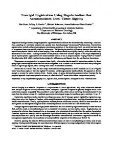
Fig. 1: Brain tissue at different resolutions. (a) Image stack acquired using a two-photon light microscope from live brain tissue at a 1 micrometer resolution and a smaller area of the same tissue imaged using an electron microscope, at a 20 nanometer resolution. The orange box in the top image denotes the area from which the EM sample has been extracted. (b) Semi-automated delineation of some dendrites overlaid in magenta and manual segmentation of an axon overlaid in green and a dendrite in yellow. (c) The segmented structures on a black background. Since the resolution is much higher in the EM data, dendritic spines and synapses are clearly visible. (d) Graph representation of the neuronal structures. The red dots, named “graph nodes”, are used for a coarse registration of the graphs. The white dots, named “edge points”, are used for fine alignment. This figure, as most others in this paper, is best viewed in color. mate, can handle non-linear deformations, and does not rely on local appearance or global distance matrices. Instead, given graphs extracted from the two images or image-stacks to be registered, we treat graph nodes as the features to be matched. We model the geometric mapping from one data set to the other as a Gaussian Process whose predictions are progressively refined as more correspondences are added. These predictions are in turn used to explore the set of all possible correspondences starting with the most likely ones, which allows convergence at an acceptable computational cost even though no appearance information is available. To make the computation tractable for large graphs, we introduce an active testing search strategy for speeding up the exploration of the set of possible correspondences by first considering the most likely ones. We demonstrate the effectiveness of our technique on a variety of registration problems including both synthetic and real data of angiographies, retinal-fundus images acquired at different times and different points of view, as well as neural image-stacks acquired using different modalities. This paper is an extended version of [31], where using Gaussian Processes was proposed, and [26], which introduced a preliminary version of the active testing strategy. The present paper combines both previous contributions, provides a more thorough mathematical justification of the active search technique, and includes a more extensive set of experiments and comparisons with other methods.

2

R ELATED W ORK

Area-based registration techniques that maximize image similarity criteria such as correlation or mutualinformation [27], [40] are not applicable in our context as they are not designed to deal with truly different appearances and limited capture ranges. We therefore consider only techniques that match graph structures across images, which we have split into four major categories. In most cases described below, only the branching points (nodes) extracted from the input structures are used for matching, while the edges connecting them are ignored. In the first class, the graphs are assumed to be related by a low-dimensional geometric transform, such as a rigid mapping, which can be instantiated from very few correspondences. It is therefore feasible to hypothesize and test random correspondences, as it is done in RANSAC [14]. However, as the number of transformation parameters or graph nodes increases, the space of possible matches becomes too large to explore randomly, and one has to resort to methods like PROSAC [10] or Guided-MLESAC [37] that reduce the search space through priors based on appearance. When appearance information is not available, more sophisticated search strategies have to be used, such as accelerated hypothesis sampling with information derived from the residual sorting [6]. Here, we propose to use an Active Search strategy [16], [26], [36], which iteratively selects the hypotheses that maximize the information gain,

SUBMITTED TO IEEE TRANSACTIONS ON PATTERN ANALYSIS AND MACHINE INTELLIGENCE

allowing to rapidly progress towards the global minimum. The second class of approaches typically requires a good initial estimate of the transformation to establish an initial estimate of the correspondences, which are then progressively refined. For rigid transformations, one of the earliest algorithms is the Iterative Closest Point (ICP) [4], later extended to non-rigid transformations using techniques such as Non-Rigid ICP [2], [21], or Coherent Point Drift (CPD) [24]. In any event, a good initial estimate is critical to prevent these methods from falling into incorrect local minima. The third class of methods relies on having a sufficiently discriminative criterion for evaluating the pairwise compatibility of nodes, such as local appearance descriptors, or the geometric compatibility when considering correspondence pairs [8], [13], [17], [19], [20], [38]. Global nodal matches are then estimated using multidimensional optimization schemes such as graduated assignment [17], spectral techniques [19], [20], [38] or considering the graphs as an absorbing Markov chain [8]. Considering compatibilities as binary tests, the largest consistent set of matches corresponds to the maximum weighted independent set or equivalently, to the maximum weighted clique [13], [32]. Due to its high computational cost, the method is only applicable to small graphs. For specific medical imaging applications, some authors have attempted to register actual biological graphs we may find in structures like the pulmonary vessels [35], or the retina [1], [12]. Yet, while these methods allow for a non-parametric formulation of the problem, they cannot be used when appearance information is not available and the inter-nodal distances vary due to non-linear deformations, which is the case we consider in this paper. The final category involves those methods that simultaneously search for correspondences and estimate the transformation parameters using a Kalman filter-like approach [7], [11], [22], [29], [33], [34]. As soon as a few initial correspondences have been established, the set of remaining potential matches is rapidly reduced, making the search complexity manageable. However, these algorithms, like RANSAC, require an a priori parametric model of the transformation whose parameters are computed using the correspondences, and thus, cannot generalize to arbitrary deformations. Similar limitations are also shared by methods relying on implicit shape models [15], [25]. In the Gaussian Process framework we propose, we also progressively reduce the number of potential correspondences but, in contrast to previous approaches, no parametric deformation model is required. Instead, the deformation is completely defined by the correspondences and can therefore be completely generic. We will demonstrate that this significantly enlarges the applicability domain of our approach and improves the accuracy of the results.

3

A PPROACH

Let us assume we are given two graphs G A = (XA , EA ) and G B = (XB , EB ), such as the one of Fig. 1-right,

3

extracted from two images or image-stacks A and B. The Es denote the graphs’ edges and the Xs their nodes— shown as red dots in the figure—that are points in RD , where we assume D ∈ {2, 3}. The edges, in turn, are represented by dense sets of points—shown as white dots in the figure—that form R2 or R3 paths connecting the nodes. Our goal is to use these two graphs to find a geometrical mapping m from A to B such that m(xA i ) is as close as possible to xB in the least-squares sense assuming that xA j i B and xj are corresponding pixels or voxels. If correspondences between points belonging to the two graphs were given, we could directly use the Gaussian Process Regression (GPR) [28] to estimate a non-linear mapping that would yield a prediction of m and its associated variance [5]. In our case, however, the correspondences are initially unavailable and cannot be established on the basis of local image information because the A and B are too different in appearance. In short, this means that we must rely only on geometrical properties to simultaneously establish the correspondences and estimate the underlying non-linear transform. Since attempting to do this directly for all edge points would be computationally intractable, our algorithm goes through the following two steps: 1) Coarse alignment: We begin by only matching graph nodes so that the resulting mapping is a combination of an affine deformation and a smooth non-linear deformation. We initialize the search by randomly picking D correspondences, which roughly fixes relative scale and orientation, and using them to instantiate a Gaussian Process (GP). We then recursively refine it as follows: Given some matches between G A and G B nodes, the GP serves to predict where other G A nodes should map and restricts the set of potential correspondences. Among these possibilities, we select the most promising one based on geometric or information gain criteria we will define in Section 5, and use it to refine the GP. Repeating this procedure recursively until enough mutually consistent correspondences have been established and backtracking when necessary lets us quickly explore the set of potential correspondences and recover an approximate geometric mapping. 2) Fine alignment: Having been learned only from potentially distant graph nodes, the above-mapping is coarse. To refine it, we also establish correspondences between points that form the edges connecting the nodes in such a way that distances along these edges, which we will refer to as geodesic distances, are changed as little as possible between the two graphs. Because there are many more such points than nodes, this would be extremely expensive to do from scratch. Therefore, we constrain the correspondence candidates to edges between already matched nodes and rely on a Hungarian algorithm [23] to perform the optimal assignment quickly. In the remainder of this paper, we first outline the GPR model that we use. We then introduce our procedures for

SUBMITTED TO IEEE TRANSACTIONS ON PATTERN ANALYSIS AND MACHINE INTELLIGENCE

Gaussian Process Regression GA, GB

Eq. (1) can now be rewritten as

Source and target graph Point in RD Dimension of the input points Set of nodes from the source graph Set of nodes from the target graph Set of GP hyperparameters Precision of the measurement noise Kernel function Number of correspondences

xi D = {2, 3} A XA = {xA 1 , ..., xnA } B } XB = {xB , ..., x nB 1 Θ = {θ0 , θ1 , θ2 , θ3 } β k (xi , xj ) nc

4

mπ (xA )

=

i=1 nc X T A = ai (θ0 + θ1 (xA i ) x )+ i=1

  nc X θ3 A 2 ai θ2 exp − ||xA − x || , (4) 2 i i=1

Active Test Search Algorithm T πt Cπt Sπt u Ω = {ω u 1 , ω0 }

ATS total number of iterations Partial assignment selected at iteration t Set of children of the tree node πt Quality score of assignment πt Scoring noise model parameters

TABLE 1: Summary of notations used in this paper

coarse and fine alignments. All the notations used in this paper are summarized by Table 1.

4

G AUSSIAN P ROCESS R EGRESSION

Without loss of generality, let us assume that the elements of XA and XB have been reordered so that the set B π = xA ↔ x l l 1≤l≤nc denotes correspondences between D-dimensional points from A and B respectively. Using the GP approach to non-linear regression and assuming Gaussian i.i.d. noise of precision β in all coordinate values, these correspondences can be used to predict that a point xB in B corresponding to xA in A can be expected to be found at a location with the following mean mπ (·) and isotropic variance σπ2 (·) : A

T

B C−1 π Xπ A A

mπ (x ) = k , σπ2 (xA ) = k (x , x ) + β −1 − kT C−1 π k ,

nc X A ai k(xA i ,x )

(1) (2)

where k is a kernel function, β −1 is the measurement noise variance, Cπ is the nc × nc symmetric matrix with A −1 elements Ci,j = k (xA δi,j , k is the vector i , xj ) + β A A A A T [k (x1 , x ), . . . , k (xnc , x )] , and XB π is the nc × D B T matrix [xB 1 , . . . , xnc ] . Among the different types of existing kernel functions [28], we chose the widely used summation of a squared-exponential, a constant term, and a linear term   θ3 k (xi , xj ) = θ0 + θ1 xTi xj + θ2 exp − ||xi − xj ||2 . (3) 2

We found this kernel to be the most appropriate for our purposes, because it implicitly defines a mapping function composed of an affine plus a non-linear transformation. This approximates well most of the warps appearing in biomedical imaging. Given this expression for k, the geometric mapping from

B where ai is the ith row of the matrix C−1 π Xπ . The first term of Eq. (4), which contains the θ0 and θ1 hyperparameters, is a linear function of the input coordinates while the second one, which involves the θ2 and θ3 , allows for additional non-linear deformations. Apart from the mapping mπ (·), we also need to evaluate the mapping quality for any particular set of correspondences π. Let us define a quality score as Sπ ∈ R, which is a deterministic function. We use the following two methods to evaluate the quality of a correspondence set: - Assigned distance: We compute the minimum possiB ble total distance between mπ (xA i ) and points xj ∈ B X for all 1 ≤ i ≤ nA

Sπ =

nA X nB X

B Hi,j · dist(mπ (xA i ), xj ),

(5)

i=1 j=1

where ‘dist’ is a Euclidean distance and H is the assignment matrix computed by the Hungarian algorithm [23]. - Number of inliers: We compute the proportion of edge and branching points in XA that are mapped near a point in XB as Sπ =

|I| , |XA |

(6)

n o A A B − 12 I = xB . j | ∃mπ (xi ), dist(mπ (xi ), xj ) < β Our experiments show that these two measures suffice to recognize good sets of correspondences.

5 C OARSE A LIGNMENT   A B Let XA = xA and XB = xB be 1 , . . . , xnA 1 , . . . , xnB the nodes of our two graphs. Our first goal is to simultaneously retrieve as many correspondences π = {xA ↔ xB } as possible and to determine the underlying non-linear mapping xB = mπ (xA ) that best aligns them. In this section, we present two different approaches for doing this. The first one—Section 5.1—relies on first assigning correspondences to nodes for which there are few to choose from. The second—Section 5.2—uses a more sophisticated strategy that ranks partial solutions and attempts to extend the most promising ones first. We introduced the first strategy in [31] and tested it successfully on relatively small graphs. However, as will be shown in Section 7, its computational requirements grow quickly with the number of graph nodes. The second strategy, while slightly more complex, scales better.

SUBMITTED TO IEEE TRANSACTIONS ON PATTERN ANALYSIS AND MACHINE INTELLIGENCE

Algorithm 1 Greedy Alignment (G A , G B ; Θ, β; T ) 1: Initialize Correspondence Set: B A B π0 ← {xA i1 ↔ xj1 , . . . , xiD ↔ xjD } 2: for t = 0, . . . , T do 3: {mπt , σπ2 t } = ComputeMapping(XA , XB , Θ, πt ) 4: Sπt = QualityScore(mπt , β) 5: for i = 1 . . . nA do 2 A B 6: Bi = ComputeBoundary(mπt (xA i ), σπt (xi ), X ) B B B B 7: PotCandi = {xj ; xj ∈ X ∧ xj ∈ Bi } 8: end for 9: i∗ = arg mini {|PotCandi |} for |PotCandi | 6= 0 10: if i∗ 6= ∅ then 11: xB j ∗ = PickRandom(PotCandi∗ ) B 12: πt+1 ← πt ∪ {xA i∗ ↔ x j ∗ } 13: else 14: πt+1 ← πt−1 15: end if 16: end for 17: return π ∗ = arg max{1,...,T } Sπt

5.1

Greedy Search

Let mπ (·) be a GP written using the formulation of Section 4, which we instantiate by first randomly selecting only D correspondences (line 1 in Algorithm 1). This gives us an initial correspondence set π0 , which we use to get a rough estimation of the global scale and rotation. We then iteratively construct sets of correspondences in T steps as follows. 1) At iteration t, we have a set of correspondences πt from which we compute (line 3) the mapping mπt (·) and covariance σπ2 t (.) using Eqs. (1) and (2). A 2) For each unmatched node xA i ∈ X , we search for B B potential correspondences xj ∈ X in the bounded region Bi determined by the predicted covariance σπ2 t (xA i ) (lines 6–7). We use the Mahalanobis distance to define the boundary:

5

The process is controlled by the noise parameter β of Eq. (2) and the vector Θ = {θ0 , θ1 , θ2 , θ3 } containing the kernel hyperparameters of Eq. (3). To avoid having to tune these parameters for each new dataset, we center and scale the XA and XB coordinates so that their average distance to the origin is one and perform the computation on the scaled datasets. As a result, we were able to use the same Θ for all experiments described in Section 7. To speed up the computation, we reject matches that would produce large changes in geodesic distances, which we define as the length of a path connecting the edges between two graph nodes xi and xj . Given already established correspondences π between graphs, then for each new potential match, the geodesic distances from the new corresponding points to the already matched nodes in both graphs have to be approximately proportional. We set the tolerance for geodesic distance variations depending on the level of deformations we expect to recover. Proceeding in this way, the algorithm gains robustness against outliers, while avoiding unnecessary checks, thus keeping a low complexity. Note that geodesic distances are invariant to rotations, to the bending of the branches, and to isometric changes. 5.2

Active Test Search

We have tested the algorithm described above on graphs containing up to 100 nodes, for which the computation takes more than 1000 seconds in Matlab on an 4-Core 2.3 GHz 64-bit processor. because the computational cost grows exponentially with the number of nodes, it becomes impractical for larger graphs. We have therefore developed an alternative approach that relies on the Active Testing Search (ATS) [16], [36]. This involves progressively refining an approximate solution by making a budgeted number of observations and computing the posterior distribution over all potential solutions after each test. Hence, the algorithm proceeds iteratively and selects at each step the correspondence set expected to yield  T  −1   B 2 A A B the highest information gain based on all previous ones. M2 = mπt (xA ) − x σ (x ) m (x ) − x πt i j πt i i j In other words, our method does not perform either n o B 2 A B a depth-first search, such as the one described in SecBi = ∀xB ∈ X |M (m (x ), x ) < 2 πt j i j tion 5.1, or a traditional breadth-first search, but a priority search. For this purpose, as new correspondences are added 3) We choose the node xA i∗ with the smallest number of potential candidates (line 9), and randomly pick one to partial solutions, it maintains a sorted list of which ones B are most likely to lead to a correct solution. It then attempts of them to define the match xA i∗ ↔ xj ∗ , which we add to the correspondence set πt (lines 11–12). If there is to extend these first so that less likely candidates may never no point from XB which satisfies the conditions to be extended at all, saving computation time. In addition, our ATS approach is adaptive and allows be selected, we remove the last added correspondence for backtracking without hand-tuned pruning of the search from πt and continue searching (line 14). 4) We take the quality score Sπt to be the number of space. It is summarized in Algorithm 2 and we describe it in more details below. inliers as defined in Eq. (6). As described in Algorithm 1, this process is repeated T times, backtracking and selecting different correspondences 5.2.1 ATS—Coarse Alignment using a depth-first search. We then return the correspon- ATS maintains a list of candidate correspondence sets, dence set π ∗ with the highest score, and its corresponding where we denote the probability that the correspondence mπ∗ . We also terminate if the inlier consenus Sπt becomes set π is part of the correct mapping π ∗ as π . This list of large enough. This process is depicted in Fig. 2. candidates is handled by means of a priority queue Q (line

SUBMITTED TO IEEE TRANSACTIONS ON PATTERN ANALYSIS AND MACHINE INTELLIGENCE

6

Original Graphs

Initialization

it#2

it#6

it#11

it#15

it#20

Coarse Alignment

Fig. 2: Coarse alignment steps. The initial graph structures are depicted in the top left-most figure, the model graph in red and the target in blue. Exploration of the search space starts by picking randomly two correspondences, highlighted in green, thus roughly fixing scale and orientation. Then, the next match candidate is chosen among the nodes located inside the bounded regions, which are a function of the GP predicted covariances, shown as black ellipses. Every correspondence added to the hypotheses set helps refining the mapping uncertainty. The final correspondence set, defines a coarse alignment of the graphs. Best viewed in color. 1 of Algorithm 2), whose elements are (π, π ) pairs sorted in order of decreasing probability. At first, we form all possible sets of D pairs of correspondences that can be used to initialize a mapping mπ (·). We assume that each π from this initial set has equal probability . At each ATS iteration, t = 0, ..., T , we want to select the candidate set πt that is most likely to provide a good mapping. We therefore select the first element (πt , πt ) of Q, which is the one with highest likelihood and then evaluate the quality score Sπt (line 5) to verify if it is indeed a good mapping. Given that Sπt can be noisy, we consider it to be a random variable with a known noise model, i.e. the likelihood model P (Sπt |π ∗ ) is assumed to be explicitly known and is described in the following section. To aggregate the information provided by the quality score, we compute the posterior distribution of the correct correspondences given the newly observed score. Simultaneously, we further refine our candidates by expanding the candidate set previously evaluated. In particular, from πt , we generate a new set of candidate correspondences B B Cπt = {πt ∪ {xA i ↔ xj }|xj 6∈ πt }, which contains all children of the current node, where xA i 6∈ πt is additional element of XA considered at the depth below πt . As in [16], [36], the posterior for any element π ∈ Cπt can be computed as r(St )πt , ∝ |Cπt |

Algorithm 2 ATS Alignment (XA , XB ; Θ, β; T, ψ) 1: Initialize Priority Queue:
B B A Q ← Push {xA i1 ↔ xj1 , . . . , xiD ↔ xjD },  2: for t = 1 . . . T do 3: {πt , t } = Pop(Q) 4: {mπt , σπ2 t } = ComputeMapping(XA , XB , Θ, πt ) 5: Sπt = QualityScore(mπt ) 6: if r(Sπt ) > ψ then return π ∗ = πt end if 7: for πz ∈ Cπt do 8: Q ← Push (πt , πt r(Sπt )/|Cπt | ) 9: end for 10: end for 11: return π ∗ = arg max{1,...,T } Sπt

following section). The complete derivation of this equation as well as why the normalization constant is not needed are shown in the Appendix. Intuitively, Eq. (7) is simply an application of Bayes rule, where πt is a prior, r(St ) is the data-term and dividing by |Cπt | attributes equal probability to all the expanded candidates of πt . Once this process is repeated T times or until the likelihood ratio is higher than ψ, we return the assignment π ∗ with the best score. 5.2.2

(7)

where r(St ) is the likelihood ratio (defined explicitly in the

Quality Score Selection and Noise Model

To compute the quality score Sπ for any set of correspondences π we use the previously described assigned distance of Eq. (5) and the number of inliers of Eq. (6). In particular,

SUBMITTED TO IEEE TRANSACTIONS ON PATTERN ANALYSIS AND MACHINE INTELLIGENCE

(a)

(b)

7

(c)

Fig. 3: Gaussian noise models for percentage of inliers. (a) Each curve depicts the Gaussian noise model N (·; ω u1 ) for a given depth u of the tree. (b) Similarly, each curve depicts the noise models for N (·; ω u0 ). (c) Likelihood ratio r(·) between N (·; ω u1 ) and N (·; ω u0 ) for each value of u.

we compute Sπ using the assigned distance when the number of correspondences |π| is below a certain threshold γ, which we set to 5 in all experiments. Otherwise we compute Sπ using the number of inliers. We found that using two different quality functions provides more informative scores for small and large sets of correspondences. This is similar to the strategies employed in [7]. We consider the quality scores to be random noisy observations and assume the following observation model ( N (s; ω u1 ), if δ(π, π ∗ ) = 1 ∗ P (Sπ = s|π ) = , (8) N (s; ω u0 ), if δ(π, π ∗ ) = 0 where π ∗ is the correct set of correspondence assignments, u is the number of correspondences in π, N is a Gaussian probability distribution with parameters ω u1 , ω u0 and δ(π, π ∗ ) = 1 if the correspondences of π respect π ∗ and 0 otherwise. From this model, the likelihood ratio can be computed as N (Sπ ; ω u1 ) . (9) r(Sπ ) = N (Sπ ; ω u0 ) To learn the parameters of the Gaussian distributions N (·; ω u1 ) and N (·; ω u0 ), we proceed as follows: - True Distribution: To estimate the parameters for N (·; ω u1 ), we synthetically generate L point clouds XA such that nB > nA and fit a minimum spanning tree to obtain the graph representation. The point cloud XB is generated by applying random affine transformations and a smaller amplitude nonlinear deformation to XA . This allows us to know exactly the true correspondence π ∗ . – generating a set {{XA }l , {XB }l , πl∗ }L l=1 . Then, we take subsets of the full set of true correspondences π ∗ and compute Sπ . Once all scores on all L generated sets are computed, we estimate the Gaussian distribution A A parameters {ω u1 }nu=1 = {µu1 , σ1u }nu=1 . An example of the learned probability densities can be seen in Fig. 3(a). - False Distribution: Second, to learn the parameters for N (·; ω u0 ), we follow a similar sampling approach. Given the number of possible incorrect correspondences, for partial assignments that include many

assignments, i.e. when u is large, we construct sets of incorrect correspondences π by starting from a subset of π ∗ and adding a few incorrectly matched points. Proceeding in this manner, we take false partial assignments which are close to the true correspondence π ∗ because we expect to only explore the higher depths of the search tree, that is, high values of u, when our previous hypotheses are correct. An example of such distribution is depicted in Fig. 3(b). In practice, we have found the above the process for learning the parameters of the observation models to be effective and robust. If enough training data with known correspondences is available, we could learn more complex models for the real shape of the positive and negative distributions. In addition, even though we use synthetically generated datasets, the same learned parameters are good enough to be used across different experiments in Sec. 7 and indicate that the parameters are fairly robust and valid for different tasks.

6

F INE A LIGNMENT

Given two graphs G A and G B , both coarse alignment algorithms described above in Sections 5.1 and 5.2 return a set of corresponding graph nodes π ∗ , along with the corresponding mapping m(·) = mπ∗ and the covariance estimator σ 2 (·) = σπ2 ∗ . This set of matches π ∗ relates the graph’s nodes and is therefore coarse. Given that the nodes are connected by paths, we can refine the mapping by establishing correspondences between edge points that lie on these paths. We assume the node correspondences to be correct and only establish new ones between points lying on paths linking matching nodes. We proceed iteratively using the following steps: 1) For each pair of paths connected by corresponding graph nodes, we use the Hungarian algorithm [23], guided by the current mapping mπr (·) and covariance estimator σπ2 r (·), to establish new matches πr+1 between the edge points of the two paths. We constrain all the matches to have a consistent geodesic distance with their respective graph nodes.

SUBMITTED TO IEEE TRANSACTIONS ON PATTERN ANALYSIS AND MACHINE INTELLIGENCE

it#1

it#2

it#3

8

Fine Alignment

Fig. 4: Fine alignment steps. Once a coarse alignment of the two graphs (model in red and target in blue) has been found, the algorithm starts matching points lying on the edges. The assignments (depicted in green) are computed using the Hungarian algorithm and constrained by the graph topology and GP predictions. After a few iterations, the warped structure (top) is completely aligned to the target graph. For each successive plot, we zoom to a smaller region (bottom) to better show the algorithm at work. Best viewed in color. 2) Given these new correspondences πr+1 , reestimate mπr+1 (·) and σπ2 r+1 (·). 3) Compute the quality of the resulting mapping Sπr+1 using the Assigned distance function defined in Eq. (5). 4) If Sπr+1 > Sπr , iterate. Otherwise, terminate and return πr , mπr (·), and σπ2 r (·). This yields a final expanded set of correspondences πf ine , mapping mπf ine (·), and covariance estimator σπ2 f ine (·). Note that we use the same GP parameters Θ as before. The whole process is illustrated by Fig. 4 and summarized in Algorithm 3.

Matching) and ATS-RGM (Active Testing Search for Robust Graph Matching), respectively. We will initially test all methods on synthetically generated data with increasing levels of noise, non-rigid deformation, missing points and different initial conditions. We will then show the performance of the algorithms on 2D and 3D biomedical images, including retinal images, neuronal structures and heart angiograms.

We will compare our algorithm to several others for nonrigid point matching and shape recovery. As representative examples of point set registration we have chosen the original Iterative Closest Point [4] (ICP), the Thin Plate SplinesAlgorithm 3 Fine Alignment (G A , G B ; Θ, β; π ∗ ) Robust Point Matching (TPS-RPM) [9], the Coherent Point 1: Initialize Correspondence Set from Coarse Alignment: Drift (CPD) [24] and the recent Gaussian Mixture Model πr = π ∗ Registration (GMMREG) proposed in [18]. As examples of mπr = mπ∗ , σπ2 r = σπ2 ∗ ; graph matching approaches, we have considered Spectral 2: repeat Matching (SM) [19] and Integer Projected Fixed Point 3: πr+1 ← OptimalAssignment(XA , XB , Θ, πr ) (IPFP) [20], which can be combined, as well as Path 4: {mπr+1 , σπ2r+1 }=ComputeMapping(XA, XB , Θ, πr+1 ) Following Algorithm (PATH) [39]. The results of the coarse 5: Sπr+1 = QualityScore(mπr+1 ) alignment obtained by ATS-RGM and our previous Greedy6: until Sπr+1 ≤ Sπr RGM version are virtually the same, therefore only the 7: return πf ine = πr results for ATS-RGM are shown when comparing accuracy.

7

E XPERIMENTS

We evaluate our approach on both synthetic and real data against state-of-the-art methods. In the remainder of the paper we will refer to the methods presented in Sections 5.1 and 5.2 as Greedy-RGM (Greedy Search for Robust Graph

We ran all the algorithms on a 2.3 GHz 4-Core 64-bit machine with 8 GB RAM. Most of the aforementioned algorithms are implemented using a combination of Matlab and Mex-C++ functions. Similarly, we implemented the skeleton of our approach in Matlab and used C++ for the most time-consuming parts: the Gaussian Process routines and the Active Testing Search.

SUBMITTED TO IEEE TRANSACTIONS ON PATTERN ANALYSIS AND MACHINE INTELLIGENCE

9

Experiment #1

Tree Model

σn = 0.01

po = 5%

Experiment #2

σn = 0.02

pd = 0.2

φ=

σn = 0.03 π 6

Tree Model

pd = 0.5

σn = 0.005

Experiment #3

Tree Model

po = 20%

σn = 0.005

po = 5%

φ=

pd = 1.5 π 6

Experiment #4

po = 40%

pd = 0.2

pd = 1.0

φ=

po = 60% π 6

Tree Model

φ=

σn = 0.005

2π 5

φ=

po = 5%

3π 5

φ=

4π 5

pd = 0.2

Fig. 5: Quantitative evaluation on synthetic data. Performance tests of all competing methods in different configurations of noise, deformation, outliers and rotation. The curves represent the median of the correct correspondences percentage achieved by each method. Below each result, we show the tree model used in all the experiments (in blue) and some corrupted samples to illustrate how each parameter affects the transformed graph (in green).

SUBMITTED TO IEEE TRANSACTIONS ON PATTERN ANALYSIS AND MACHINE INTELLIGENCE

-

Fig. 6: Computational Cost. Processing time required by RANSAC, Greedy-RGM and ATS-RGM as a function of the number of nodes. We computed the median of 20 experiments for each of the methods.

7.1

-

Synthetic Experiments

To evaluate our approach against others, we generated pairs of trees composed of a model tree computed as the minimum spanning tree of N = 50 randomly selected 2D points in a 2 × 2 bouding box and target tree obtained by deforming and randomizing it. More specifically, let xi be the nodes of the model tree and x0i those of the target tree. For all i from 1 to N , we write x0i = R(φ)

 Sx 0

   0 T xi + x + D(pd ) + ξ(σn ), Ty Sy

(10)

where the deformation includes the following components. - Rotation, scaling, and translation; The target model is rotated by an angle φ, translated by Tx and Ty , and scaled by Sx and Sy - Non-linear deformation: We add a non-linear warping D(pd ) defined as a linear combination of B-splines whose control points are uniformly distributed in the input space. Its magnitude is controlled by pd , which specifies the amount of displacement of the B-spline coefficients. - Noise: We perturb the node locations of the target graph by a zero mean Gaussian noise ξ(σn ), where σn is the standard deviation. - Outliers: We produce outliers by randomly and independently removing a percentage po of the total number N of nodes from both the model and target trees. As a result, some branches appear in one tree and not the other. We use the pairs of trees created in this manner as input to all algorithms. To ensure a fair comparison, we set the required parameters to the values suggested in the corresponding papers, which we list below1 . - ICP: Does not require extra parameters. - TPS-RPM: We set the initial temperature Tinit to half the maximum Euclidean distance between the 1. Note that for ease of reference we are keeping the same parameter notation here as in the original papers. While some of these parameters are also used in our algorithm (i.e. : w, T , σd ) their meaning do not necessarily need to be the same.

10

nodes of the model tree, and the final temperature to Tf inal = 0.01 · Tinit . The remaining parameters are set to λinit = 1 and λinit = 0.01, as suggested by the 1 2 authors. GMMREG: We set the maximum number of iterations to 10000, and α and β to 1 and 2, respectively. CPD: We use a non-rigid configuration of the algorithm for all the experiments. We set λ = 3, β = 3 and outliers = 0.2. SM and IPFP: We build the affinity matrix using the description provided in [19]. As we do not have appearance information, we set the label affinity term M (a, a) to zero, making the matching score depend solely on the pairwise geometric information. The (d −d 0 0 )2 pairwise affinity is set to M (a, b) = 4.5 − ij 2σ2i j d if |dij − di0 j 0 | < 3σd and zero otherwise. PATH: We build the graphs as suggested by the authors for the application of “alignment of vessel images”. We connect each node xi to all points xj within a distance r, and each edge is assigned a weight wi,j = exp(−||xi − xj ||2 ), ∀xi , xj ∈ X, ||xi − xj ||2 < r. This is done for all nodes of both model and target trees. In our case we set r = 0.3 · dmax , where dmax is the maximum Euclidean distance between the points of the model tree.

7.1.1

Performance Evaluation

We tested all algorithms for robustness to rotation, deformation, and topology changes by varying the geometric deformation parameters of Eq. (10) as well as the percentage of missing nodes p0 . We performed four different independent experiments. For each we generated 50 pairs of model and target trees using the same set of parameters and a fixed small change in scale and translation. In Experiment #1 we evaluated the influence of noise on the points 2D locations by sweeping the range σn ∈ [0 – 0.04] and setting po = 5%, pd = 0.2 and φ = π6 . In Experiment #2 we tested the behavior of the algorithms against increasing levels of non-linear deformation, varying the deformation parameter within the range pd ∈ [0 – 2], and setting the rest of parameters to constant values σn = 0.005, po = 5%, and φ = π6 . Similarly, in Experiment #3, we assessed the robustness of the algorithms to the presence of outliers by randomly deleting a percentage po ∈ [0% − 90%] of nodes in both trees –which turned to outlier tree branches– and setting σn = 0.005, pd = 0.2 and φ = π6 . Finally, in Experiment #4 we tested the invariance of all the methods to initial conditions by changing the orientation of the target within φ ∈ [−π, π] and fixing the rest of the parameters to σn = 0.005, po = 5% and pd = 0.2. To give significance to the magnitudes of the experimental parameters we consider, the images below each performance curve of Fig. 5 show different samples of the same model graph and different target graphs generated by varying the levels of noise, deformation, outliers and rotation. For each experimental parameter setting experiments and each algorithm, we computed the average percentage of

SUBMITTED TO IEEE TRANSACTIONS ON PATTERN ANALYSIS AND MACHINE INTELLIGENCE

11

X: 1048 Y: 498.8

(a)

(b)

(c)

(d)

(e)

(f)

Fig. 7: Retinal fundus images used in [12]. Each row contains a single experiment. (a,b) Two images of the same retina taken from different viewpoints, with the vascular trees overlaid in red and blue. (c) The first tree is overlaid in red over the second image after non-linear transformation, which corresponds to the output of the Greedy-RGM coarse alignment. (d) Final result of our non-rigid registration: the graph from the first image is overlaid in red over the second image. (e) Our result is superposed with the Coherent Point Drift alignment, in yellow. (f) Detail of the rectangle in (e). Our algorithm behaves well on this dataset, while CPD fails to recover the correct shape because there are too many non-corresponding branches. Best viewed in color.

(a)

(b)

(c)

(d)

(e)

(f)

Fig. 8: Angiography images from a beating heart. (a) Two different images with extracted vascular trees overlaid in red. (b) Two other images taken later in the heart cycle with extracted vascular trees overlaid in blue. (c) The original red trees are shown after the non-linear coarse alignment of the tree nodes, obtained using our Greedy-RGM. (d) The resulting warped trees are overlaid in red after non-linear registration. Note that the trees —in particular in the first example— have distinctly different topologies, which affects our algorithm very little. (e) Comparison with the result obtained using non-linear Coherent Point Drift, in yellow. (f) A zoom of a region of interest. Using the graph intrinsic geometry grants us robustness against vessel bendings and outliers, achieving a better registration of the two shapes. Best viewed in color.

correct matches over our 50 tree pairs and plot the results in Fig. 5. Under favorable conditions, that is, relatively small graphs with less than 50 nodes, uncorrupted data and purely affine transformation, all methods exhibit similar performance. However, when we progressively introduce artifacts the differences become clear. For instance, it can be seen that CPD deals poorly when there are missing parts or when the initial rotation is above 70 degrees, as stated in their paper. Similarly, the rigid ICP can only find local solutions, even when dealing with much smaller initial rotation angles. Graph methods (PATH, SM+IPFP) are able to find global solutions as they are invariant to

initial conditions by construction. However, as shown in the first row of Fig. 5, they are very sensitive to modifications in the topology of the graph. TPS-RPM and GMMREG underperform our approach for each of the tests. In short, each one of the competing methods can address some of the difficulties, however only ours can handle all of them. The results of Fig. 5 also indicate the suitability of using our approach in sub-graph matching. The robustness of our approach stems from the randomized search strategy, that allows searching for a global minimum and makes the algorithm insensitive to initial rotations. This is true for both Greedy and Active Testing Search. On the other hand,

SUBMITTED TO IEEE TRANSACTIONS ON PATTERN ANALYSIS AND MACHINE INTELLIGENCE

(a)

(b)

(c)

12

(d)

(e)

Fig. 9: Blood vessels in brain tissue. (a) Segmented two photon microscopy data. (b) Segmented bright-field optical microscopy data. (c) Registration of structures using Active Testing Search, in red. (d) Alignment using CPD, in yellow. (e) A view in detail at the results of both ATS-RGM and CPD. Best viewed in color.

(a)

(b)

(c)

(d)

(e)

Fig. 10: Light and electron microscopy neuronal trees. (a) Graph structure extracted from the electron microscopy image stack, in red. (b) Segmented light microscope neurons in blue. (c) After the non-linear registration process using ATS-RGM, the EM segmented neuron is deformed and aligned over the LM extracted neuron. (d) Registration using CPD, in yellow, which falls into a local minimum. (e) A zoom over the region where the EM stack has been extracted. The two neurons have been completely aligned. Best viewed in color.

the non-rigid transformation based on Gaussian Process regression provides robustness to large amounts of noise and deformation. 7.1.2 Computational Cost Finally, we compared the computational cost of the two versions of our algorithm and RANSAC [14]. We generated a new set of experiments in which the new model and target tree pairs are as before except for the fact that we varied the number of nodes from 20 to 200 and performed an affine transformation plus random noise of small amplitude. As illustrated in Fig. 6, the computation time grows much faster for both Greedy-RGM and RANSAC than for ATS-RGM, which remains manageable. Both versions of our algorithm (ATS-RGM and Greedy-RGM) yield similar performance, only differing in the time consumed to reach the global solution. Note that, since the transformations are almost affine, the absolute run-time value is lower than some of the real experiments we consider in the next section. Note that the purely local methods, such as CPD and ICP, tend to be much faster and can deal with thousands of points in reasonable amounts of time. Yet, as we have seen in the fourth experiment of Fig. 5, these algorithms require accurate initializations. On the other hand, the graph matching methods, such as SM + IPFP or PATH, treat the problem as an Integer Quadratic Program (IQP) and hence are limited by the construction of the pairwise score matrix whose size grows quadratically with the number of nodes.

7.2

Real Experiments

We next present several examples of results obtained by ATS-RGM and Greedy-RGM on real biomedical datasets. The graphs were extracted semi-automatically using a plugin [3] for the Fiji platform [30]. To evaluate the accuracy of the different methods in the absence of ground truth, we assigned each node in the deformed graphs —overlaid in red for our method and yellow for CPD on Figs. 7 and 8 (d,e,f)— to its assumed match in the target graph overlaid in blue. To this end, we use the Hungarian algorithm to find it by taking the Euclidean distance as the cost to minimize, while rejecting outlier branches by setting a distance threshold defined ad hoc for each of the datasets. We use this error measure since there is no true correspondence between the sampled points along the edges of the graphs. This error measure gives an idea of the quality of the alignment. Observe for example, the assignments (in green) obtained in the two images of Fig. 11, for the Greedy-RGM and CPD methods. In Table 2, we show these errors and the corresponding computation times. For ATS-RGM and Greedy-RGM, we distinguish the times required for coarse and fine alignment. We have not provided the error for IPFP and PATH because these methods only give correspondence hypotheses, and are unable to define a valid transformation without an outlier rejection step. In Fig. 7 we show registration results for retinal fundus vascular graphs that are deformed from one image to

SUBMITTED TO IEEE TRANSACTIONS ON PATTERN ANALYSIS AND MACHINE INTELLIGENCE

ATS-RGM

Greedy-RGM

CPD [24]

ICP [4]

TPS-RPM [9]

GMMREG [18]

(pix) (s) (pix) (s) (pix) (s)

2.68 1293.3 + 406.4

2.68 5998.9 + 336.8

20.67∗ 580.2

20.04∗ 24.3

19.32∗ 4236.8

21.30∗ 139.7

2.94 280.0 + 301.4 1.16 307.8 + 129.4

2.51 16353.1 + 261.2 1.05 1240.9 + 162.8

20.45∗ 468.5 2.95 144.3

20.46∗ 67.9 9.77∗ 8.1

17.79∗ 5791.1 2.92 726.7

20.84∗ 147.1 4.21 31.9

(pix) (s) (vox) (s)

1.57 167.9 + 77.2 4.38 593.7 + 55.5

1.81 112.0 + 95.4 4.89 15029.1 + 19.9

3.42 68.8 4.19 37.1

4.84∗ 5.0 7.23 30.9

3.21 327.0 6.67 334.8

6.56 21.1 12.71 31.2

Error (µm) Time (s)

0.05 42.4 + 15.8

0.07 116.1 + 18.2

0.25∗ 22.2

0.27∗ 28.2

0.20∗ 28.5

0.46∗ 22.4

Dataset Retina I (Fig. 7 Top) Retina II (Fig. 7 Bot.) Angio I (Fig. 8 Top) Angio II (Fig. 8 Bot.) Brain vessels (Fig. 9) Neuronal (Fig. 10)

13

Error Time Error Time Error Time Error Time Error Time

TABLE 2: Error: Geometric error on real datasets for the proposed approach and other state of the art methods. Failed experiments (producing incorrect alignment) are marked with an *, see Fig. 7(d) or Fig. 10(d) for examples. Elapsed Time: Processing time for each method, in seconds. For ATS-RGM and Greedy-RGM, we distinguish the times required for coarse and fine alignment.

the next because the camera is looking from different viewpoints. This produces distortions of the curved retinal surface’s projection, that are well modeled by an affine transform. Thus, there is very little non-linearity in the deformation and these results are similar to those of [12], even though the trees only partially overlap. However, as the amount of spurious branches is quite large, CPD fails to recover the correct shape. In contrast, our approach can naturally handle such artifacts. In the 2D X-ray angiography images of Fig. 8 the nonlinearities of the transformation are much more apparent. As shown in the zoomed-in area, our algorithm nevertheless does a good job of recovering this more complex deformation and aligning the trees. Again, we assessed the performance of the CPD on these images and observed that it could not retrieve a correct solution unless a relatively accurate initialization was provided. Even when we supplied with our coarse transformation estimate, CPD could only deal with small non-linearities. Next, we register two 3D datasets. A blood vessels network in brain tissue is shown in Fig. 9. One of the 3D image stacks is acquired using a two-photon microscope and the other using bright-field microscopy after excision and fixation. As the resulting segmentations are partially aligned, the experiment’s difficulty consists in identifying the non-linearities of the deformation. Our algorithm clearly outperforms other state-of-art methods and provides results similar to the CPD. In the zoomed image of Fig. 9(e) it is possible to appreciate it. Although CPD works well when the initial conditions are favorable, it completely misaligns one of the branches while our result respects the topology. Finally, we register the 3D neuronal stacks extracted from the brain tissue of Fig. 1 using light (LM) and electron (EM) microscopy, where the EM block is a small section of the LM volume and has been non-linearly deformed due to the extracting process. The intended application is to automatically localize the EM volume in the corresponding part of the LM volume. Even though the two images look extremely different, our algorithm returns a valid deformation as shown in Fig. 10. No other method was able to recover the correct alignment.

(a)

(b)

Fig. 11: Accuracy Measure. Two alignment solutions computed from the retina dataset by Greedy-RGM (a) and CPD (b). The assignments (in green) between the points of the two graphs after registration are used to compute the residual distance error. Best viewed in color.

8

C ONCLUSION

We have shown that our algorithm can match graphs with neither appearance information nor initial pose estimate, while allowing for partial matches and non-linear deformations. This is made possible by using Gaussian Processes to model the geometric mapping from one graph to another and using this mapping to progressively constrain the search area for correspondences between graph nodes. Because this mapping is non-parametric, we can effectively handle situations containing high levels of non-linear deformations with many nodes and without assuming any particular transformation model beforehand. For relatively small graphs a simple depth-first approach to establishing the correspondences yields good results. As the graphs become bigger, the set of all possible correspondences becomes too large and we therefore proposed a more sophisticated approach that ranks partial solutions and attempts to extend the most promising ones first. This allows to correctly align biological structures that are non-linearly transformed and extracted with different techniques, without the need of prealigning them, in a manageable amount of time. We have also shown in quantitative experiments that our method consistently outperforms stateof-the-art.

SUBMITTED TO IEEE TRANSACTIONS ON PATTERN ANALYSIS AND MACHINE INTELLIGENCE

As future work, we will explore how we can include graph constraints to further reduce the computational cost of the search, allowing for a registration of bigger nonlinear structures.

R EFERENCES [1]

[2] [3] [4] [5] [6] [7] [8] [9] [10] [11] [12] [13] [14]

[15] [16] [17] [18] [19] [20]

[21] [22] [23]

W. Aguilar, Y. Frauel, F. Escolano, M. Elena Martinez-Perez, A. Espinosa-Romero, and M. Angel Lozano. A Robust Graph Transformation Matching for Non-Rigid Registration. Image and Vision Computing, 27:897–910, 2009. B. Amberg, S. Romdhani, and T. Vetter. Optimal Step Nonrigid ICP Algorithms for Surface Registration. In Conference on Computer Vision and Pattern Recognition, 2007. F. Benmansour, E. Turetken, and P. Fua. Tubular Geodesics: Fiji plugins, 2012. http://cvlab.epfl.ch/software/delin/index.php. P. Besl and N. Mckay. A Method for Registration of 3D Shapes. IEEE Transactions on Pattern Analysis and Machine Intelligence, 14(2):239–256, February 1992. C.M. Bishop. Pattern Recognition and Machine Learning. Springer, 2006. T. Chin, J. Yu, and D. Suter. Accelerated Hypothesis Generation for Multistructure Data via Preference Analysis. IEEE Transactions on Pattern Analysis and Machine Intelligence, 34(4):625–638, 2012. M. Chli and A.J. Davison. Active Matching. In European Conference on Computer Vision, pages 72–85, 2008. M. Cho, J. Lee, and K.M. Lee. Reweighted Random Walks for Graph Matching. In European Conference on Computer Vision, pages 492– 505, 2010. H. Chui and A. Rangarajan. A New Point Matching Algorithm for Non-Rigid Registration. Computer Vision and Image Understanding, 89(2-3):114–141, 2003. O. Chum and J. Matas. Matching with Prosac - Progressive Sample Consensus. In Conference on Computer Vision and Pattern Recognition, pages 220–226, June 2005. A.J. Davison. Active Search for Real-Time Vision. In International Conference on Computer Vision, pages 66–73, 2005. K. Deng, J. Tian, J. Zheng, X. Zhang, X. Dai, and M. Xu. Retinal Fundus Image Registration via Vascular Structure Graph Matching. International Journal of Biomedical Imaging, 2010. O. Enqvist, K. Josephson, and F. Kahl. Optimal Correspondences from Pairwise Constraints. In International Conference on Computer Vision, 2009. M.A Fischler and R.C. Bolles. Random Sample Consensus: A Paradigm for Model Fitting with Applications to Image Analysis and Automated Cartography. Communications ACM, 24(6):381–395, 1981. K. Fujiwara, K. Nishino, J. Takamatsu, B. Zheng, and K. Ikeuchi. Locally Rigid Globally Non-Rigid Surface Registration. In International Conference on Computer Vision, 2011. D. Geman and B. Jedynak. An Active Testing Model for Tracking Roads in Satellite Images. IEEE Transactions on Pattern Analysis and Machine Intelligence, 18(1):1–14, January 1996. S. Gold and A. Rangarajan. A Graduated Assignment Algorithm for Graph Matching. IEEE Transactions on Pattern Analysis and Machine Intelligence, 18:377–388, 1996. B. Jian and B. C. Vemuri. Robust Point Set Registration Using Gaussian Mixture Models. IEEE Transactions on Pattern Analysis and Machine Intelligence, 33(8):1633–1645, 2011. M. Leordeanu and M. Hebert. A Spectral Technique for Correspondence Problems Using Pairwise Constraints. In International Conference on Computer Vision, pages 1482–1489, October 2005. M. Leordeanu, M. Hebert, and R. Sukthankar. An Integer Projected Fixed Point Method for Graph Matching and Map Inference. In Advances in Neural Information Processing Systems, pages 1114– 1122, 2009. H. Li, R.W. Sumner, and M. Pauly. Global Correspondence Optimization for Non-Rigid Registration of Depth Scans. In Symposium on Geometry Processing, pages 1421–1430, 2008. F. Moreno-Noguer, V. Lepetit, and P. Fua. Pose Priors for Simultaneously Solving Alignment and Correspondence. In European Conference on Computer Vision, October 2008. J. Munkres. Algorithms for the Assignment and Transportation Problems. Journal of the Society of Industrial and Applied Mathematics, 5(1):32–38, March 1957.

14

[24] A. Myronenko and X.B. Song. Point-Set Registration: Coherent Point Drift. IEEE Transactions on Pattern Analysis and Machine Intelligence, 32(12):2262–2275, 2010. [25] N. Paragios, M. Rousson, and V. Ramesh. Non-Rigid Registration Using Distance Functions. Computer Vision and Image Understanding, pages 142–165, 2003. [26] M. A. Pinheiro, R. Sznitman, E. Serradell, J. Kybic, F. MorenoNoguer, and P. Fua. Active Testing Search for Point Cloud Matching. In Information Processing in Medical Imaging, 2013. [27] J. P. W. Pluim, J. B. A. Maintz, and M. A. Viergever. Mutual Information Based Registration of Medical Images: A Survey. IEEE Transactions on Medical Imaging, 22(8):986–1004, 2003. [28] C. E. Rasmussen and C. K. Williams. Gaussian Process for Machine Learning. MIT Press, 2006. [29] J. Sanchez-Riera, J. Ostlund, P. Fua, and F. Moreno-Noguer. Simultaneous Pose, Correspondence and Non-Rigid Shape. In Conference on Computer Vision and Pattern Recognition, June 2010. [30] J. Schindelin, I. Arganda-Carreras, E. Frise, V. Kaynig, M. Longair, T. Pietzsch, S. Preibisch, C. Rueden, S. Saalfeld, and B. Schmid. Fiji: an open-source platform for biological-image analysis. Nature Methods, 9(7):676–682, 2012. Code available at http://pacific.mpicbg.de. [31] E. Serradell, P. Glowacki, J. Kybic, F. Moreno-Noguer, and P. Fua. Robust Non-Rigid Registration of 2D and 3D Graphs. In Conference on Computer Vision and Pattern Recognition, June 2012. [32] E. Serradell, F. Moreno-Noguer, J. Kybic, and P. Fua. Robust Elastic 2D/3D Geometric Graph Matching. In SPIE Medical Imaging, 2012. [33] E. Serradell, M. Özuysal, V. Lepetit, P. Fua, and F. MorenoNoguer. Combining Geometric and Appearance Priors for Robust Homography Estimation. In European Conference on Computer Vision, pages 58–72, September 2010. [34] E. Serradell, A. Romero, R. Leta, C. Gatta, and F. Moreno-Noguer. Simultaneous Correspondence and Non-Rigid 3D Reconstruction of the Coronary Tree from Single X-Ray Images. In International Conference on Computer Vision, November 2011. [35] D. Smeets, P. Bruyninckx, J. Keustermans, D. Vandermeulen, and P. Suetens. Robust Matching of 3D Lung Vessel Trees. In MICCAI Workshop on Pulmonary Image Analysis, 2010. [36] R. Sznitman and B. Jedynak. Active Testing for Face Detection and Localization. IEEE Transactions on Pattern Analysis and Machine Intelligence, 32(10):1914–1920, June 2010. [37] B. Tordoff and D.W. Murray. Guided Sampling and Consensus for Motion Estimation. In European Conference on Computer Vision, pages 82–98, 2002. [38] L. Torresani, V. Kolmogorov, and C. Rother. Feature Correspondence via Graph Matching: Models and Global Optimization. In European Conference on Computer Vision, pages 596–609, 2008. [39] M. Zaslavskiy, F. Bach, and J-P. Vert. A Path Following Algorithm for the Graph Matching Problem. IEEE Transactions on Pattern Analysis and Machine Intelligence, 31(12):2227–2242, 2009. [40] B. Zitova and J. Flusser. Image Registration Methods: A Survey. Image and Vision Computing, 11(11):977–1000, 2003.