Soichiro Inatani, Truyen Van Phan and Masaki Nakagawa. Department of Information ..... 18 Average of lengths of spatial neighbors. 19 Standard deviation of ...
2014 14th International Conference on Frontiers in Handwriting Recognition
Comparison of MRF and CRF for Text/Non-text Classification in Japanese Ink Documents Soichiro Inatani, Truyen Van Phan and Masaki Nakagawa Department of Information Engineering Tokyo University of Agriculture and Technology Tokyo, Japan inai17ibar @ gmail.com, truyenvanphan @ gmail.com, nakagawa @ cc.tuat.ac.jp
For training and evaluating pattern recognition and classification systems, a massive amount of samples is necessary. There are two popular online handwritten document databases, the Kondate database [1] and the IAMonDo database [3]. They are used in most of the researches on text/non-text classification. Kondate has Japanese online handwritten documents containing text, drawings, diagrams, formulas, etc. IAMonDo stores English online handwritten documents containing heterogeneous objects similarly.
Abstract— In the paper, we compare the methods based on Markov Random fields (MRF) and Conditional Random fields (CRF) for separating text and non-text ink strokes in online handwritten Japanese documents. This paper validates the effect of context information in neighbor strokes based on graphical models of MRF and CRF. The task of separating text and nontext ink strokes in ink documents denotes classifying ink strokes into two classes (text and non-text). For classification, Support Vector Machine (SVM) classifiers are trained on the set of ink strokes. After converting the SVM’s outputs to likelihood probabilities, they are assigned to the likelihood clique potentials of MRF and the feature functions of CRF. The classification based on MRF or CRF is considered as a labeling problem, which can be solved using a labeling algorithm. The experiments on Japanese ink documents in the Kondate database shows that the proposed method based on CRF achieves a classification rate of 98.02% while the method based on MRF produces the classification rate of 97.86%. Keywords— Text/Non-text classification; Text/Non-text separation; ink stroke classification; Markov Random fields; MRF; Conditional Random fields; CRF
I.
(a)
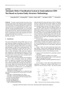
Fig. 1. An example of online handwritten digital ink from the Kondate database [1], with non-text strokes highlighted in green.
INTRODUCTION
In recent years, several works using context information reported superior results for text/non-text classification. Context information comes not only from each stroke but also from its surrounding strokes. For example, there is context related to the position of strokes and the time relation to write a sequence of strokes. Zhou et al. [5] achieved high classification rate (96.61%) for Japanese documents in the Kondate database. It proposed the approach for classifying text and non-text based on Markov Random fields (MRF), which utilized the spatial relationship in neighboring strokes. The result was superior to that of the classification by SVM (92.58%). Delaye et al. [6] presented the state-of-the-art performance for English documents in the IAMonDo database. The method based on Conditional Random field (CRF) achieved 96.68%, which utilized the spatial and temporal relationship. Similarly, Delaye et al. [7] proposed the method based on Conditional Random fields (CRF) with 5 types of relationship. It achieved higher performance (97.23%) than the result of [6]. However, we cannot compare [5] and [7] under the same condition due to the differences of the databases and the number of features. In [6] and [7], new features called local context features carry context information in its surrounding strokes. Recently, the new approach for mode detection using long short-term memory
As smart phones and tablet PCs spread into both home and workplace, people are getting accustomed to touch-based or pen-based interfaces. These devices allow users to write text and draw figures on their surfaces in the form of pen-tip or finger-tip traces, often called digital ink, without changing mode so that a user is able to express one’s idea or concept naturally and explain it to others who can also understand it without paying any attention. On the other hand, mixture of text, tables, diagrams, formulas and whatever else in digital ink brings about a difficult problem to document analysis and recognition systems. For machine recognition and information retrieval, those mixed objects need to be classified into abstract classes such as text, tables, diagrams and formulas. Text/nontext classification improves text recognition, text search [2], diagram interpretation [3] and so on. Figure 1 shows an example of mixed or heterogeneous digital ink from the Kondate database [1]. In order to realize high performance and effectiveness of succeeding recognition and interpretation, text/non-text classification must produce high accuracy without taking large processing time.
2167-6445/14 $31.00 © 2014 IEEE DOI 10.1109/ICFHR.2014.120
(b)
684
are called TT_SVM, NN_SVM and TN_SVM. The TT_SVM classifies each stroke pair into two classes: text&text or the rest. The text&text class indicates that a pair of strokes is classified into text. Similarly, NN_SVM classifies each stroke pair into non-text&non-text or the rest. TN_SVM classifies each stroke pair into text&non-text or the rest. The results of the binary SVMs have context information, which can be used to improve classification accuracy.
(LSTM) [8] presented outstanding performance (98.47%) than other methods for the IAMonDo database. The method utilized only temporal relationship without the use of spatial relationship. As we can see from these previous works, context information is important for improving the results of text/nontext classification. In this paper, we propose the two methods based on MRF and CRF for classifying ink strokes into text and non-text in online handwritten Japanese documents. The purpose of this work is to compare the methods under the same condition for the same database and fairly evaluate their performances.
C. Classification based on the graphical model Markov Random Fields (MRF) and Conditional Random Fields (CRF) are probabilistic graphical models, which have Markov property and can express the interactions between classes of neighbor strokes. We perform the reclassification based on MRF and CRF to the outputs by the SVMs. It is necessary to convert the outputs of the SVMs to suitable values. In this work, we input them as clique potentials on the graphical models.
This paper is organized as follows. Section II describes the proposed classification methods based on MRF or CRF. Section III presents the feature extraction of single strokes and stroke pairs. Section IV presents the MRF model in this paper and its parameters estimation. Then, Section V presents the CRF model and how to train it. Section VI presents the experiments and their results. Finally, Section VII draws conclusions of this paper. II.
Following [5], the output of U_SVM is converted to posterior probabilities for text class and non-text class. Then, the outputs of the three binary SVMs are converted to posterior probabilities for three classes: text&text, nontext&non-text, and text&non-text. By fitting sigmoid functions, the SVMs’ outputs are converted to posterior probabilities. For M class classification, the outputs of M SVMs are converted to posterior probabilities in (1), where ߙ is the bias for class ݆ (�݆ ൌ ͳ to )ܯ, ߚ is the weight.
CLASSIFICATION METHODS
The text/non-text classification problem can be formulated as a labeling problem. Figure 2 shows the system architecture for text/non-text classification based on which we compare the constituent methods and elaborate them. It is composed of three parts, feature extraction, stroke classification and context evaluation in term of the graphical model: MRF or CRF model. First, we introduce how to extract features from strokes in online documents. Second, we present the classification of single strokes and that of stroke pairs by Support Vector Machine (SVM) classifiers. Finally, we classify each ink stroke into text or non-text according to MRF or CRF based on results of the SVMs. In the rest of this section, we briefly present the system architecture. Text/non-text classification
Input data
Online Handwritten document
Feature Extract
Stroke Classification (SVM Classifier)
Context Evaluation (Graphical Model)
ߨ ሺ݂ሻ ൌ ܲ൫ߨ ൌ ͳห݂൯ ൌ
ͳ ͳ �ሾെሺߚ ݂ ߙ ሻሿ
ሺͳሻ
These parameters are estimated by minimization of the cross-entropy function [10][11] in (2). ே
ெ
ܬൌ െ ൣ�ݐ �ߨ ൫ͳ െ ݐ ൯ ൫ͳ െ ߨ ൯൧
Output data
ሺʹሻ
ୀଵ ୀଵ Classification Result
According to the Bayesian rule, the posterior probabilities can be converted to conditional likelihood probabilities in (3), where ݔis a set of features. ܲሺݐሻ is the prior probability for class ݐ, which is estimated from a training set.
Fig. 2. The system for text/non-text classification.
A. Extraction Stroke Features We extract 2 types of features from ink strokes for text/nontext classification. The first type of features is called unary stroke features, which are extracted from single strokes. The second type of features, binary stroke features, is extracted from pairs of strokes. Unary stroke features are used for single stroke classification into text or non-text, and binary stroke features are used for pair stroke classification into three classes as described in the next sub-section.
ܲሺݔȁݐሻ ൌ
ܲሺݐȁݔሻܲሺݔሻ ܲሺݐȁݔሻ ן ܲሺݐሻ ܲሺݐሻ
ሺ͵ሻ
By the Gibbs distribution, the unary likelihood probability ܲሺݔ ȁ݆ሻ is converted to the single-stroke likelihood clique potential in (4), where is the unary stroke feature. Similarly, the binary likelihood probability ሺݔ ᇲ ȁ݆ǡ ݆Ԣሻ is converted to the likelihood clique potential in (5), where ݔ ᇲ is the binary stroke feature. The clique potentials are proportional to negative logarithm of probabilities and monotone decreasing functions, which can be summable.
B. Classification by SVM In [9], SVM classifiers are used to evaluate both the stroke features. We train and test 4 SVMs. The first SVM called U_ SVM, which classifies each single stroke into two classes: text and non-text. The result of U_SVM presents text/non-text classification accuracy without context information. Then, three other SVMs classify stroke pairs into three classes: text&text, non-text&non-text, and text&non-text. Their SVMs
ܸଵ ሺݔ ȁ݆ሻ ൌ െ ܲሺݔ ȁ݆ሻ ǡ ݆ ܮ א ܸଶ ሺݔᇱ ȁ�݆ǡ ݆ ᇱ ሻ ൌ െ ܲሺݔ ᇲ ȁ݆ǡ ݆ ᇱ ሻ ǡ ݆ǡ ݆Ԣ ܮ א
685
ሺͶሻ ሺͷሻ
The prior clique potentials are also proportional to negative logarithm of prior probabilities of five classes: text, non-text, text&text, non-text&non-text, and text&non-text. Equation (6) shows the single-stroke prior clique potential, where ݒ Ͳ�is the penalty against a stroke classified into class�݆. Equation (7) shows the pair-stroke prior clique potential, where ݒை௧ ݒூௗ Ͳ indicates that spatial neighbor strokes often belong to the same class. They have an effect of controlling the rate of strokes classified into each class. ܸଵ ሺ݆ሻ ൌ ݒ �ǡ����݆ �ܮ א
C. Binary Stroke Feature Table 2 shows three sets of binary stroke features in previous works. Only 4 binary stroke features are used in [5] and 6 binary stroke features are used in [6]. Delaye et al. [7] extracts 20 binary stroke features, where the first 13 features focus on the gap between neighboring strokes and the last 7 features measure the similarity between them. To compare performances of three sets of unary and binary stroke features, we experiment with them respectively. TABLE I.
ሺሻ ሺሻ
[5] 1 2 3 4
[6] 1 2 3 4
This section presents how to make cliques, two neighborhood systems and all the features.
5 6 7 8 9 10 11
5 6 7 8
ܸଶ ሺ݆ǡ ݆
ᇱሻ
ݒ ����݆��݆Ԣ��
ൌ ൜ ூௗ ݒை௧ ����������݆ǡ ݆Ԣ ܮ א
III.
FEATURE EXTRACTION
A. Cliques and Neiborhood Systems Strokes in online ink documents correspond to the set of observed sites�ܵǣ� ݔൌ ሼݔଵ ǡ ǥ ǡ ݔூ ሽǡ ݅ ܵ א. The classes correspond to the set of labels� ܮൌ ሼܶǡ ܰሽ, which are text (ܶ) and non-text ( ܰ ). The labeling to assign the sites is expressed as � ݕൌ ሼݕଵ ǡ ǥ ǡ ݕூ ሽǡ ݕ ܮ אǡ ݅ ܵ א, which is estimated by a labeling algorithm.
9 10
11 12
13
To make context tractable, two types of the cliques, singlesite cliques and pair-site cliques, are taken into account in this work. The single-site cliques are defined by only a site. The pair-site cliques are defined by two sites selected according to a neighborhood system. The neighborhood system decides whether or not strokes are adjacent. We use two neighborhood systems based on spatial relationship and temporal relationship.
14
[7] Feature Description 1 Stroke length. 2 Area of the convex hull of the stroke. Compactness. Eccentricity. 3 Stroke duration. 4 Ratio of the principal axis of the stroke seen as a cloud of points. 5 Rectangularity of the minimum area bounding rectangle of the stroke. 6 Circular variance of points of the stroke around the principal axis. 7 Normalized centroid offset along the principal axis. 8 Ratio between first-to-last point distance and trajectory length. 9 Accumulated curvature. 10 Accumulated squared perpendicularity. 11 Accumulated signed perpendicularity. 12 Stroke width. 13 Stroke height. 14 Number of temporal neighbors of the stroke. 15 Number of spatial neighbors of the stroke. 16 Average of the distances from the stroke to spatial neighbors. Standard deviation of the distances from the stroke to spatial 17 neighbors. 18 Average of lengths of spatial neighbors. 19 Standard deviation of lengths of spatial neighbors. Average of the distances from the stroke to spatial neighbor’s centroid.
TABLE II.
The spatial neighborhood system is used for making pairsite cliques. The spatial neighborhood system decides whether or not strokes are neighbors according to the minimum distance between strokes, that is, only the strokes within a certain distance are considered as neighbors. With reference to [5], the threshold is set to 0.4 times the average stroke length of a training set.
[5] 1 2 3
[6] 1 2 3
4
4
5 6
The temporal neighborhood system is also used for extracting binary stroke features and local context, which is a part of unary stroke features mentioned below. Two strokes are temporal neighbors if the temporal distance between them is below a threshold 3.5 (in seconds) and if they are not separated by more than 4 intermediate strokes between them in the time sequence. B. Unary Stroke Feature Table 1 presents three sets of unary stroke features in previous works. Only 11 unary stroke features are used in [5] and 14 unary stroke features are used in [6]. In Delaye et al. [7], 19 unary stroke features including local context are extracted. The first 13 features have properties of each single stroke itself, whereas last 6 features called local context have properties of its spatial and temporal neighboring strokes.
THREE SETS OF UNARY STROKE FEATURES.
THREE SETS OF BINARY STROKE FEATURES.
[7] Feature Description 1 The minimum distance between two strokes. 2 The maximum distance between the endpoints of two strokes. 3 The minimum distance between the endpoints of two strokes. The distance between the centers of the bounding boxes of two strokes. 4 Horizontal distances of the centroids of 2 strokes. 5 Vertical distances of the centroids of 2 strokes. 6 Off-stroke distance between 2 strokes. 7 Off-stroke distance projected on X and Y axis. 8 Temporal distance between 2 strokes. 9 Ratio between off-stroke distance and temporal distance. Ratio between areas of the largest bounding box of 2 strokes and that 10 of their union. 11 Number of strokes in the sequence between 2 strokes. Number of spatial neighbors of 2 strokes intersecting the bounding 12 box defined by centroids of 2 strokes. Number of spatial neighbors of 2 strokes intersecting the line joining 13 the centroids. 14 Ratio between areas of the bounding boxes. 15 Ratio between the lengths of the diagonal of the bounding boxes. 16 Ratio between the heights of the bounding boxes. 17 Ratio between the widths of the bounding boxes. 18 Ratio between the stroke curvatures. 19 Ratio between the stroke lengths. 20 Ratio between the stroke durations.
IV.
MARKOV RANDOM FIELDS
Figure 3 depicts an example of the graphs by Markov Random Fields (MRF), where ܰ is adjacent to a site�݅. The interactions between labels of neighboring sites represent
686
Therefore, maximizing a posterior probability in (8) is equivalent to minimizing the energy function in (13). In this work, the energy function is minimized according to the relaxation labeling (RL) Algorithm [12], so that we can find the best labeling by solving�� כ ݕൌ ���ܷሺݔȁݕሻ.
posterior distributions. MRF has a restriction that the interdependence of labels is governed only by labels of neighboring sites defined by the neighborhood system [12]. To solve the classification problem as a sequence labeling problem, we use the MAP-MRF framework in reference to [5].
ܷሺݔȁݕሻ ܷሺܨሻ ൌ ሼܸଵ ሺݔȁݕሻ ܸଵ ሺݕሻሽ� ଵאଵ
������������������������������� ሼܸଶ ሺݔȁݕሻ ܸଶ ሺݕሻሽ
ሺͳͶሻ
ଶאଶ
B. Parameters Estimation The results of the 4 SVMs can be approximately converted to the likelihood clique potentials. The prior clique potentials are the parameters of MRF, which depend on the prior probabilities for each class. However, it is difficult to calculate the prior probabilities directly because the interactions between labels of sites spread globally. In this paper, we estimate their parameters using the Genetic Algorithm (GA). GA has higher precision than a gradient descent algorithm, while it takes a longer time than a gradient descent algorithm. We choose GA for improving accuracy. Here we set the parameters on genes respectively. The range of each parameter is decided with respect to the parameter in [5]. The fitness function to evaluate is a classification rate on a training set.
Fig. 3. An example of the graphs by Markov Random Fields.
A. MAP-MRF Framework In the MAP-MRF framework, we can find the best labeling כ ݕunder an optimization criterion, which is usually the maximum a posteriori (MAP) probability. Equation (8) shows the maximization of a posterior probability. כ ݕൌ ܲሺݕȁݔሻ ൌ ܲሺݔȁݕሻܲሺݕሻ ௬
௬
ሺͺሻ
According to the Hammersley-Clifford theorem, MRF can be seen as the Gibbs random field [12]. In (9), ܲሺݕሻ denotes the prior probability for each label.�The normalization function ܼ guarantees the probabilistic nature. In (10), ܷሺݕሻ indicates the prior energy function, which is a sum of the prior clique potentials on a clique�ܿ. ͳ ିሺ௬ሻ ݁ ܼ
ሺͻሻ
ܷሺݕሻ ൌ ܸ ሺݕሻ
ሺͳͲሻ
ܲሺݕሻ ൌ
V.
With reference to [5] and [7], we propose a simpler method than the method in [7] with a less number of weights and feature functions.
א
Equation (11) demonstrates the probability of (8) is represented by the energy function. In (12), the likelihood energy function ܷሺݔȁݕሻ is calculated from the likelihood clique potentials under the conditional independence of observed sites. ܲሺݔȁݕሻܲሺݕሻ ൌ
ͳ ିሺሺ௫ȁ௬ሻାሺ௬ሻሻ ݁ ܼ
ܷሺݔȁݕሻ ൌ ܸ ሺݔȁݕሻ
A. Formulation In (15), we can find the best labeling according to maximizing the conditional probability ܲሺݕȁݔሻ , where ߰ indicates a potential function on a clique �ܿ . The potential functions are formed of feature functions and weight parameters. Equation (16) presents a normalization function that guarantees the probabilistic nature of (15).
ሺͳͳሻ
ሺͳʹሻ
א
ܲሺݕȁݔሻ ൌ
By the Bayesian rule, (13) presents the posterior energy function, which is derived from the likelihood energy and the prior energy. In (12), ܥindicates a set of all cliques. ܷሺݕȁݔሻ ܷ ןሺݔȁݕሻ ܷሺݕሻ ൌ ሼܸ ሺݔȁݕሻ ܸ ሺݕሻሽ
CONDITIONAL RANDOM FIELDS
Conditional Random Field (CRF) represents a distribution over labels conditioned on the observation as MRF [13]. It has a structure of the graphical model and can express contextual dependency from probabilities between random variables directly. It is important to design potential functions composed of feature functions and weight parameters to use CRF.
ͳ ෑ ߰ ሺݕ ǡ ݔ ሻ ܼሺݔሻ
ሺͳͷሻ
ீא
ܼሺݔሻ ൌ ෑ ߰ ሺݕԢ ǡ ݔ ሻ
ሺͳሻ
௬ᇱא ீא
ሺͳ͵ሻ
CRF has a property to have some weight parameters that can be trained. In [7], the number of feature functions and that of weight parameters are both 82. We design the model containing 7 weight parameters�ࣂ and 10 feature functions. The feature functions of [7] employ 20 binary stroke features while
א
Equation (14) shows the posterior energy is composed of the likelihood clique potentials and the prior clique potentials on single-sites and pair-sites where �ͳܥis a set of single-site cliques and ʹܥis a set of pair-site cliques.
687
best labeling כ ݕin accordance with maximizing a conditional posterior probability ܲሺݕȁݔሻ using the ICM method.
ours employ clique potential functions �ࢂ derived from the outputs of the three binary SVMs. The proposed model is less expressive than [7], but it can be easily trained.
VI.
Equation (17) presents the single-site clique potential function, where ܸଵ ሺݔ ȁ݆ሻ is a likelihood single-site clique potential for label �݆�ሺܮ אሻ , and ܸଵ ሺ݆ሻ is a prior single-site clique potential for a label�݆ . Then, (18) shows a pair-site clique potential function, where a label�݆Ԣ�ሺܮ אሻ denotes the label of a site ݐneighbored to site� ݏ. In (18), ܸଶ ሺݔᇱ ȁ�݆ǡ ݆ ᇱ ሻ indicates a likelihood pair-site clique potential, and ܸଶ ሺ݆ǡ ݆ ᇱ ሻ indicates a prior pair-site clique potential.
A. Database To evaluate performances of the proposed methods employing MRF and CRF, we use Japanese ink documents in the Kondate database, which contains 670 documents pages by 67 writers, 10 pages of each writer. In [5], 310 pages were used for training and 360 pages were used for testing. We follow these sets in order to compare our results with their results rather than making cross validation. In this experiment, we train the 4 SVM classifiers, MRF and CRF. Table 3 summarizes the number of document pages and strokes for training and testing, and breakdown of strokes into text and non-text strokes.
The above mentioned 7 weight parameters adjust biases between these feature functions. In (17), �ߠ௨ �and�ߠ adjust the bias for single-site and pair-site cliques. In (18), ߠ௩ and ᇱ ߠ௩ adjust the biases for five classes: text, non-text, text&text, non-text&non-text and text&non-text. There are constraints ܸଶ ሺݔᇱ ȁ�ܶǡ ܰ�ሻ ൌ ܸଶ ሺݔᇱ ȁ�ܰǡ ܶ�ሻǡ���ܸଶ ሺܶǡ ܰሻ ൌ ܸଶ ሺܰǡ ܶሻ and ߠ௩்ே ൌ ߠ௩ே் Ǥ ߰ ൫ݕ ǡ ݔ Ǣ ߠ ǡ ߠ௩ ൯ ൌ
൛ߠ௨ �ܸଵ ሺݔ ȁ݆ሻ
ߠ௩ �ܸଵ ሺ݆ሻൟ
TABLE III.
THE NUMBER OF DOCUMENT PAGES AND STROKES FOR TRAINING AND TESTING IN THE KONDATE DATABASE.
Usage Training Testing
ሺͳሻ
ᇲ
ሺͳͺሻ
B. Training Parameters In CRF, training is equivalent to optimizing the weight parameters ࣂ for bias adjustment. Equation (20) shows a labeling criterion of maximizing the pseudo-likelihood (PL) of the ground truth labeling on a training set. Equation (19) presents PL of each site�݅, where ܰ is adjacent to a site�݅, and ݕே is the label of a site �ܰ . The computation of the denominator involves summing over the labels of a single site�ݕԢ .
ሺͳͻሻ
TABLE IV.
�ሼܲ ሺݕ หݔǡ ݕே Ǣ ࣂ൯ሽ ࣂ
Text 51681 61969
Non-text 9869 10793
T (%) 83.97 85.18
N (%) 16.03 14.82
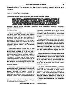
Figure 4 depicts the results shown in Table 4. U_SVM and TT_SVM improve remarkably from the small set of features to the larger set, while NN_SVM and TN_SVM are almost unchanged. It is necessary to review binary features related to non-text strokes. MRF with 4 SVMs performs middle for the small set of features and does best for the large set. Its effect for the large feature set seems reasonable but its unclear effect for the small set must be analyzed.
For MRF, we employed GA, but we could not get the best parameters for CRF, so that we employed BFGS for CRF. ςא ߰ ሺݕ ǡ ݔ ሻ � σ௬ᇱ ςא ߰ ሺݕԢ ǡ ݔ ሻ
#Strokes 61550 72752
Table 4 shows results by 4 SVMs and MRF with all of 4 SVMs employing the three sets of features. The experiment shows the effect of adding features. MRF with 4 SVMs for the largest set of features performs best (97.86%). We need to test whether more features may improve the classification.
The maximization of PL is performed by a gradient descent algorithm (the limited memory BFGS method) shown in [14]. In this paper, we also estimate 7 weight parameters ࣂ using a gradient descent algorithm.
ܲ ሺݕ หݔǡ ݕே Ǣ ࣂ൯ ൌ
#Pages 310 360
B. Results We use the 4 SVM classifiers with the RBF kernel function because it has higher versatility than other kernel functions. As the result of training, ்ݒis set to 0.084 and ݒே is set to 0.856 for single-site prior clique potentials. We set ݒூௗ ൌ ͲǤ͵ͷ͵ and ݒை௧ ൌ ͵ǤʹͲͷ for pair-site prior clique potentials. The number of neighboring strokes has the average 6.496 and the variance 21.01 on a training set. The crossover method of GA is the two-point crossover, with the crossover rate being 0.80 and the mutation rate being 0.15.
��߰ ൫ݕ௦ ǡ ݕ௧ ǡ ݔ௦ ǡ ݔ௧ Ǣ ߠ ǡ ߠ௩ ൯ ൌ ቄߠ ܸଶ ሺݔᇱ ȁ�݆ǡ ݆ ᇱ ሻ ߠ௩ ܸଶ ሺ݆ǡ ݆ ᇱ ሻቅ
EXPERIMENTS
ሺʹͲሻ
RESULTS OF THE CLASSIFICATION METHODS BY 4 SVMS AND MRF EMPLOYING THE THREE SETS OF FEATURES.
� � � Feature set Methods U_SVM (%) TT_SVM (%) NN_SVM (%) TN_SVM (%) SVMs +MRF (%)
ௌ
C. Testing The problem of exact inference in CRF is intractable. In this paper, we adopt the iterated conditional mode (ICM) method [12] to solve it. The ICM method is a simple algorithm, which can be easily handled by making local approximations of the global probability distribution. Therefore, we find the
1st Set [5] (U:11 B:4 ) 92.79 95.56 95.95 97.13 95.70
2nd Set [6] (U:14 B:6 ) 94.71 96.33 95.93 97.11 96.53
3rd Set [7] (U:19 B:20 ) 96.71 97.22 96.11 97.15 97.86
U: Number of unary stroke features, B: Number of binary stroke features
688
98% 97% 96% 95% 94% 93% 92% 1st Set U_SVM TN_SVM
2nd Set TT_SVM SVMs+MRF
training set by the Genetic Algorithm, and the parameters of CRF are estimated by the gradient descent algorithm. We have experimented on the Kondate database. The method employing CRF achieved a classification rate of 98.02%, while the method employing MRF achieved 97.86%. Therefore, CRF is considered to utilize context information more effectively than MRF, due to the fact that CRF expresses a distribution of labels of sites directly by training the weight parameters.
3rd Set NN_SVM
Remaining work includes feature selection and combination, cross validation, application to other databases and examination of experiment conditions.
Fig. 4. Classification results by 4 SVMs and MRF employing the three sets of features.
ACKNOWLEDGMENT
Next, Table 5 shows the results by MRF and CRF with 4 SVMs for the best set (the 3rd set) of features. We can see that the classification rate by CRF is slightly higher than that by MRF. This implies that CRF utilizes context information more effectively than MRF, since CRF expresses a distribution of labels of sites directly. The results are slightly superior to the previous works [5][6][7], but, they are at least 0.5 inferior to LSTM in [8].
The authors would like to thank Dr. Bilan Zhu for giving helpful comments and suggestions. REFERENCES [1]
[2]
Compared with U_SVM, MRF and CRF classify non-text strokes remarkably higher, but their non-text classification rates are still low. We need to improve non-text classification. [3]
There remains a considerable amount of work to be made. We should test combinations of all the features and employment of more features. We should also consider other neighborhood systems and elaborate the structures of MRF and CRF. Experiment on the three sets of features should be made not only for MRF but also for CRF.
[4]
In this study, we split sample patterns into training and testing sets to compare our results with the previous work. In order to increase the reliability of the comparison, we need to make cross validation with estimation error.
[5]
[6]
The language dependence must be also studied. IAMonDodatabase for English documents must be tried. Moreover, the experiment condition must be examined. We pursued the best for MRF and CRF separately, which produced differences for their training. TABLE V.
Rate (%) Time (s) Rate (%)
[7]
[8]
RESULTS OF THE CLASSIFICATION METHODS BY MRF AND CRF USING THE BEST SET OF FEATURES. U_SVM 96.71 0.02 Text Non-text 99.21 82.05
SVMs +MRF 97.86 0.89 Text Non-text 98.91 91.65
SVMs +CRF 98.02 0.99 Text Non-text 99.15 91.02
[9] [10]
[11]
VII. CONCLUSION In this paper, we have compared the two models MRF and CRF for text/non-text classification in online handwritten Japanese documents. We integrated a set of features and employed a spatial neighborhood system for all the experiments. The likelihood clique potentials of MRF and the feature functions of CRF are derived from the results of 4 SVM classifiers. The parameters of MRF are estimated on the
[12] [13]
[14]
689
K. Mochida, and M. Nakagawa, “Separating Figures, Mathematical Formulas and Japanese Text from Free Handwriting in Mixed On-Line Documents,” International Journal of Pattern Recognition and Artificial Intelligence (IJPRAI), vol.18, no.7, pp.1173-1187, 2004. T. Matsushita, C. Cheng, Y. Murata, B. Zhu and M. Nakagawa, “Effect of Text/Non-text Classification for Ink Search Employing String Recognition”, in Proceeding of the 10th IAPR International Workshop on Document Analysis Systems (DAS2012), Gold Cost, QLD, pp.27-29, 2012. M. Bresler, D. Průša, and V. Hlaváč, “Modeling Flowchart Structure Recognition as a Max-Sum Problem”, in Proceedings of the 12th International Conference on Document Analysis and Recognition (ICDAR2013), Los Alamitos, USA, pp.1247-1251, 2013. E. Indermühle, M. Liwicki, and H. Bunke, “IAMonDo-database: An Online Handwritten Document Database with Non-uniform Contents,” in Proceedings of the 9th International Workshop on Document Analysis Systems (DAS2010), Boston, USA, pp.97-104, 2010. X.D. Zhou, and C.L. Liu, “Text/Non-text Ink Stroke Classification in Japanese Handwriting Based on Markov Random Fields,” in Proceedings of the 9th International Conference on Document Analysis and Recognition (ICDAR2007), Curitiba, Brazil, pp.377-381, 2007. A. Delaye, and C.L. Liu, “Text/Non-Text Classification in Online Handwritten Documents with Conditional Random Fields,” in Proceedings of the Chinese Conference on Pattern Recognition (CCPR2012), Beijing, China, pp.514-521, 2012. A. Delaye, and C.L. Liu, “Contextual tex/ non-text stroke classification in online handwritten with conditional random fields”, Pattern Recognition, Volume 47, Issue 3, pp.959-968, 2014. S. Otte, D. Krechel, M. Liwicki and Andreas Dengel, “Local Feature based Online Mode Detection with Recurrent Neural Networks”, in Proceedings of the 12th International Conference on Frontiers in Handwriting Recognition (ICFHR2012), Bari, pp.533-537, 2012. V. N. Vapnik, “Statistical Learning Theory”, John-Wiley Press, 1998. J. Platt, “Probabilistic outputs for support vector machines and comparisons to regularized likeli-hood methods,” Advances in Large Margin Clas-sifiers, A.J. Smola, P. Bartlett, D. Scholkopf, D. Schuurmanns (Eds), MIT Press, 1999. C.L. Liu, “Classifier Combination Based on Confidence Transformation,” Pattern Recognition, vol.38, no.1, pp.11–28, 2005. Stan Z. Li, “Markov Random Field Modeling in Image Analysis”, Springer, 2001. J. Lafferty, A. McCallum, F. Pereira, “Conditional random fields: probabilistic models for segmenting and labeling sequence data“, in: Proceedings of the International Conference on Machine Learning (ICML2001), pp.282–289, 2001. D. Liu,J. Nocedal, “On the limited memory BFGS method for large scale optimization”, MathematicalProgramming 45, pp.503–528, 1989.