Non-uniform Compressive Sensing in Wireless Sensor Networks ...

Non-uniform Compressive Sensing in Wireless Sensor Networks: Feasibility and Application Yiran Shen∗# , Wen Hu∗ , Rajib Rana∗ , Chun Tung Chou# ∗

CSIRO ICT centre, Australia

{wen.hu,rajib.rana}@csiro.au #

School of Computer Science and Engineering, UNSW, Australia {yrshen,ctchou}@unsw.edu.au

Abstract—In this paper, we consider the problem of using wireless sensor networks (WSNs) to measure the temporal-spatial profile of some physical phenomena. We base our work on two observations. Firstly, most physical phenomena are compressible in some transform domain basis. Secondly, most WSNs have some form of heterogeneity. Given these two observations, we propose a non-uniform compressive sensing method to improve the performance of WSNs by exploiting both compressibility and heterogeneity. We apply our proposed method to a real WSN data set. We find that our method can provide a more accurate temporal-spatial profile for a given energy budget compared with other sampling methods.

I. INTRODUCTION In this paper, we consider the problem of using wireless sensor networks (WSNs) to measure the temporal-spatial profile of some physical phenomena in an energy efficient manner. Much work [7], [5], [17] has been done in improving the efficiency of WSNs in the past decade. The key distinction of this paper is that we exploit compressibility and heterogeneity to derive a non-uniform compressive sensing method to improve the performance of WSNs. More specifically, the non-uniform compressive sensing method that we propose can give a more accurate temporal-spatial profile for a given energy budget compared with other methods. Our work is based on two hypotheses. Firstly, we assume that most physical phenomena are compressible in some transform domain basis. This is also the assumption behind the recently proposed theory of compressive sensing (CS), which is an efficient signal reconstruction method that can recover a signal from a small number of samples [3], [2]. This is also the assumption behind a number of recent work [1], [4] on using compressive sensing to improve the operations of WSNs. Secondly, we assume that each WSN has some form of heterogeneity. For example, in a multi-hop WSN, different nodes require different amount of energy to forward packets to the sink due to their relative position to the sink. Nodes that are far away from the sink will only need to relay few packets for other nodes while nodes close to the sink will need to relay more packets for other nodes [9]. It is also possible that nodes choose transmission power adaptively based on the local link quality observations [10], resulting in different nodes requiring different amount of energy to forward packets to the sink.

Given these two hypotheses, we propose a non-uniform compressive sensing (NCS) method to improve the performance of WSNs by exploiting both compressibility and heterogeneity, and evaluate the proposed NCS extensively with a real WSN application dataset, which features resource consumption heterogeneity. Furthermore, we present a distributed implementation of NCS framework that introduces very little communication overheads, and show that, compared to previously proposed approach based on and sparse approximation [14], NCS achieves similar signal approximation accuracy but with significantly less energy consumption. The rest of this paper is organized as follows. Section II discusses assumptions (compressible signals and resource heterogeneity) and describes the proposed NCS architecture. In Section III, we discuss the basic set-up of the problem and the background knowledge of CS, which is followed by the introduction of the notion of NCS in Section IV. We evaluate and study proposed NCS framework by a dataset from a WSN deployment in Section V. We discuss prior work in Section VI. Finally, Section VII concludes the paper. II. A SSUMPTIONS AND NCS A RCHITECTURE A. Assumptions WSNs are deployed to obtain an accurate temporal-spatial profile of some physical phenomena, e.g., temperature, humidity, wind speed, and/or wind direction [12], [18]. In this paper, we make the following two assumptions on the behavior of WSNs for NCS architecture. Assumption 1: The signals (or physical phenomena) monitored by WSNs are compressible in some transform domains. Common examples of transform domains include DCT, wavelets or Haar wavelet. Assumption 1 implies that the sampling frequency of sensors is high enough to capture any temporal correlation in the usually slowly-varying underlying environmental state of interest [15], and we will formally defined compressible signal in Section III. Assumption 2: There is heterogeneity, e.g., the energy supply (harvest) rate and/or energy consumption rate, in the WSNs, and we can exploit the heterogeneity to increase the performance (e.g., increase network duty cycles and lifetime) of WSNs.

2

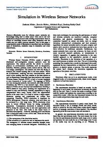
For example, energy-rich nodes can be sampled with higher rate compared to energy-constrained nodes, which may extend the battery life of energy-constrained nodes and, thereby the lifetime of the WSN can be extended. We believe that these two assumptions are not restrictive at all and can be satisfied by most WSNs. We will introduce an application in Section V, which shows that NCS exploits the energy consumption heterogeneity of nodes to reduce network energy consumption. B. NCS Architecture Fig. 1 shows the architecture of NCS. The NCS middleware takes the application/user policy (signal accuracy requirement) as external input. Based on these inputs, the sample scheduler decides the sampling parameters, such as the number of samples that needs to be collected from a WSN and some global parameters such as network energy supply or consumption rates, and informs individual nodes. At a sampling instance, a node will decide whether to take a sample or not based on the output of a local random number generator with a non-uniform probability distribution, which takes the sampling parameters and some local information such as node energy supply or consumption rate as input. If a sample is taken by a node, the sample is forwarded to the base station. These samples are used to recover the monitored physical phenomena by the reconstruction module. When there is a significant difference between the number of collected samples and the number of requested samples, the reconstruction module will inform the sample scheduler which will in turn notify individual nodes by changing sample parameters. An important argument that we will make in the following section is that, due to the heterogeneity of the WSNs, the probability distribution for making sampling decision should be non-uniform. Furthermore, we will demonstrate that nonuniform sampling has a better performance compared with uniform sampling.

Fig. 1.

System architecture.

III. BASIC SET- UP AND BACKGROUND ON COMPRESSIVE SENSING

We point out in the previous section that heterogeneity in resource supply or resource consumption is a common phenomenon in WSNs. Given this heterogeneity in resource supply or consumption in WSNs, we propose that non-uniform sampling can be a tool that we can exploit to improve the performance in such WSNs. In particular, we want to show that, by using non-uniform sampling, we can, for a given energy budget, improve the accuracy of the temporal-spatial profile obtained from WSNs. In order to realise this goal, we need to develop a model to understand how non-uniform sampling affects the accuracy of the temporal-spatial profile obtained. If we have such a model and if we also know the energy consumption of a particular non-uniform sampling pattern, then we will be able to determine good sampling patterns that give accurate temporalspatial profile for a given energy consumption. Therefore, in Section IV, we will develop a model to show how non-uniform sampling affects the accuracy of the temporal-spatial profile. The model that we will develop uses compressive sensing as the building block. The aim of this section is two-fold. Firstly, we present a basic set-up of the problem and review some results in compressive sensing which is necessary for the development in Section IV. We begin with setting up the problem. Consider a wireless sensor network with N nodes where each node measures a number of physical phenomena, e.g. temperature, humidity, wind speed, wind direction. We will consider one physical phenomenon at a time. Let xit denote the value of a particular physical phenomenon at sensor i (where i = 1, ..., N ) and time t (where t = 1, ..., T ). The complete temporal-spatial profile of a physical phenomenon consists of n = N T values of xit with i = 1, ..., N and t = 1, ..., T . It is obviously good to have the complete temporal-spatial profile since this provides the maximum amount of information. However, this means that all sensor nodes will need to sample at all time and this can result in high sampling or transmission energy consumption. In order to lower the energy consumption, we do not require all the sensors to sample the physical phenomenon at all time. If the value of a physical phenomenon xjτ is not measured (or sampled) by sensor j at time τ , we will predict the value of xjτ from those sensor readings that are available. In the following discussion, we will collect all the values of xit into a n×1 vector x where each element of x corresponds to the value of the physical phenomenon at a particular sensor at a particular time. We will assume some of the elements of the vector x are known (i.e. an element of x is known if the corresponding sensor samples at the corresponding time) and the goal is to predict the unknown elements of x from those that are known. A key idea behind the prediction method is to exploit the fact that most physical phenomena are compressible in some transform basis, e.g. Fourier, DCT, wavelets etc. A signal x ∈ Rn is said to be compressible in a transform basis Ψ, if the coefficients of the x in the basis Φ decays according

3

to the power law. In order to define this more precisely, we specify a transform basis Ψ by a n × n matrix Ψ whose columns are the basis vectors. In this case, the coefficients of x in the basis Ψ is given by the vector g where x = Ψg. Let us rearrange the elements in g in decreasing order of magnitude, |g|(1) ≥ |g|(2) ≥ ... ≥ |g|(n) , then x is compressible if the following condition holds: |g|(k) ≤ Ck −p ∀k = 1, .., n

(1)

for some p ≥ 1 [3] and some constant C. We will use data collected from real wireless sensor networks to show that physical phenomena such as temperature and humidity are compressible in spatial domain. We now explain how compressive sensing method, such as the one described in [2], can be used to estimate the unknown elements in x from those that are known. We first introduce the concept of sampling matrix, denoted by Φ. Let us assume that m elements of x are known and the indices of these m elements in x are k1 , k2 , ..., km . Let Ω be the set of the indices of the samples, i.e. Ω = {k1 , k2 , ..., km }. Let also I ∈ Rn×n denote the identity matrix. We define IΩ be a m-by-n matrix such that the k-th row of I is also a row in IΩ if k ∈ Ω. With this definition, the vector IΩ x ∈ Rm contains the known elements of x. The compressive sensing method in [2] says that one can estimate the unknown elements in x given IΩ x (i.e. the known elements in x) and the fact that x is compressible in the transform domain Ψ by solving the following linear programming problem: x ˆ = Ψˆ y where y ˆ = arg minn kyk1 s.t. IΩ Ψy = IΩ x y∈R

(2)

For the case where the vector x is sparse (i.e. most of the elements of the coefficients of x in the transform domain Ψ is zero), [2] gives some theoretical results on how the probability of recovering the vector x successfully depend on m, see [2] for further details. The compressive sensing method described above assumes that exactly m out of n (where m