different node densities and the non-uniform grid structure that best extends network .... Figure 5.2 GUI developed for simulation of the test area and the routing ...
NON UNIFORM GRID-BASED COORDINATED ROUTING IN WIRELESS SENSOR NETWORKS Priyanka Kadiyala, B.Tech.
Thesis Prepared for the Degree of MASTER OF SCIENCE
UNIVERSITY OF NORTH TEXAS JUNE 2008
APPROVED: Robert Akl, Major Professor Ram Dantu, Committee Member Parthasarathy Guturu, Committee Member Krishna Kavi, Chair of the Department of Computer Science and Engineering Dr. Oscar Garcia, Dean of the College of Engineering Sandra L. Terell, Dean of The Robert B. Tolouse School of Graduate Studies
1
Acknowledgements I would like to express my heartfelt gratitude to my major professor Dr. Robert Akl for his belief in me and the support extended by him throughout my work. It has been a wonderful experience to work under his guidance and I am very much thankful to him for it. I would also like to thank my committee members Dr. Ram Dantu and Dr. Parthasarathy Guturu for their invaluable help and advise in bringing my work together. I would further extend a grateful thanks to Dr. Murali Varanasi, Dr. Kamesh Namuduri and Dr. Savitha Namuduri, for without their support my thesis would not have been possible. A very special thanks to Sarma Varanasi, Naren Kanukolanu and Nitya Kandukuri. Finally, I thank my parents and my sister for their unconditional love and support throughout.
2
Priyanka Kadiyala, Non-uniform Grid-based Coordinated Routing in Wireless Sensor Networks Master of Science (Computer Science and Engineering), June 2008, 71 pp. 1 Table, 30 Figures. Wireless sensor networks are ad hoc networks of tiny battery powered sensor nodes that can organize themselves to form self-organized networks and collect information regarding temperature, light, and pressure in an area. Though the applications of sensor networks are very promising, sensor nodes are limited in their capability due to many factors. The main limitation of these battery powered nodes is energy. Sensor networks are expected to work for long periods of time once deployed and it becomes important to conserve the battery life of the nodes to extend network lifetime. This work examines non-uniform grid-based routing protocol as an effort to minimize energy consumption in the network and extend network lifetime. The entire test area is divided into non-uniformly shaped grids. Fixed source and sink nodes with unlimited energy are placed in the network. Sensor nodes with full battery life are deployed uniformly and randomly in the field. The source node floods the network with only the coordinator node active in each grid and the other nodes sleeping. The sink node traces the same route back to the source node through the same coordinators. This process continues till a coordinator node runs out of energy, when new coordinator nodes are elected to participate in routing. Thus the network stays alive till the link between the source and sink nodes is lost, i.e., the network is partitioned. Our work explores the efficiency of the non-uniform grid-based routing protocol for different node densities and the non-uniform grid structure that best extends network lifetime.
3
CONTENTS Acknowledgements
2
List of Tables
7
List of Figures
8
CHAPTER 1. INTRODUCTION
11
1.1 The Sensor Node
12
1.1.1 Components of a Sensor Node
12
1.2 Hardware and Software
14
1.3 Problem Description and Motivation
14
1.4 Objectives
15
1.5 Contributions
16
1.6 Organization
16
CHAPTER 2. ROUTING PROTOCOLS FOR WIRELESS SENSOR NETWORKS
19
2.1 Introduction
19
2.2 Traditional Routing Protocols
20
2.3 Ad-hoc Routing Protocols
22
2.4 Related work
24
2.5 Conclusions
30
CHAPTER 3. FLOODING, GAF AND SPAN
31
3.1 The Flooding Algorithm
31
3.2 Motivation
33
3.3 Geographic Adaptive Fidelity
34
3.4 SPAN
35
4
CHAPTER 4. UNIFORM AND NON UNIFORM GRID BASED ROUTING
37
4.1 Grid-based Coordinated Routing
37
4.2 Non Uniform Grid-based Coordinated Routing
40
4.3 Non-uniform grid-based routing protocol
41
4.4 The Link Models
43
4.4.1 Deterministic Link Model
44
4.4.2 The Probabilistic Link Model
44
4.5 Determining the grid size
46
4.6 Grid coordinator election
47
4.7 Load Balancing
49
4.8 Conclusions
51
CHAPTER 5. SIMULATIONS AND RESULTS
52
5.1 Assumptions
52
5.1.1 The Energy Model
52
5.1.2 Simulation of the sensor field and deployment of nodes
54
5.2 Parameters affecting routing in the network
59
5.3 Analyzing the results
61
5.4 Uniform node deployment
63
5.5 Random node deployment
66
5.6 Results
68
5.7 Comparison with Traditional Flooding Algorithm
73
5.8 Analysis of Results
74
CHAPTER 6. CONCLUSIONS
77
5
6.1 Summary
77
6.2 Future Research
78
BIBLIOGRAPHY
79
6
List of Tables Table 1. Comparison of network lifetime for uniform and non-uniform grid structures 75
7
List of Figures Figure 1.1 Wireless Sensor Network ................................................................................ 11 Figure 1.2 Architecture of a sensor node .......................................................................... 12 Figure 3.1 Simulation topology showing the traditional flooding algorithm. .................. 32 Figure 4.1The uniform grid structure of grid-based coordinated routing protocol........... 39 Figure 4.2 The uniform grid structure with 100 sensor nodes deployed uniformly in the field………………………………………………………………………………………39 Figure 4.3 Topology showing the alternating non-uniform grid structure called the alternate structure with 100 nodes uniformly deployed across the field and alternate small grids of 100 m each side, and large grids of 200 m each side…………………………...41 Figure 4.4 Simulation topology showing the source non-uniform structure with 100 sensor nodes deployed uniformly in the field wherein the area containing the source node is divided into small grid sizes of 100 m each, while at the sink node the area is divided into grids of size 200 m each…………………………………………………………….42 Figure 4.5 Simulation topology showing the sink non-uniform grid structure with 100 nodes deployed uniformly across the field, wherein the vicinity around the source node is divided into 200 m sized grids while the area in the vicinity of the sink node is divided into 100 m sized grids……………………………………………………………………43 Figure 4.6 Probabilistic link model………………………………………………………44 Figure 4.7 Simulation topology showing nodes having greater than 25% of battery life, marked in green ; nodes having less than or equal to 25% of battery life in yellow ; nodes with zero battery life in red………………………………………………………………48 Figure 4.8 Simulation topology showing node election by maximum node ID………....49
8
Figure 4.9 Topology showing load balancing in the network………………………… 51 Figure 5.1 Topology showing the energy depletion of nodes........................................... 54 Figure 5.2 GUI developed for simulation of the test area and the routing protocol……..55 Figure 5.3 Snapshot of flooding in the GUI……………………………………………..56 Figure 5.4 Uniform deployment of sensor nodes across the field when source node is in 200 m sized grids and sink node is in 100 m sized grids………………………………...57 Figure 5.5 Simulation topology showing random deployment of 100 and 1000 nodes in the field when the source node is in 100 m sized grids and the sink node is in 200 m sized grids………………………………………………………………………………………58 Figure 5.6 Different parameters affecting performance of the sensor network................ 60 Figure 5.7 Graph showing the transmissions for each successful link established between the source and the sink nodes. The Y-axis denotes the count of the transmissions while the X-axis denotes the time for which the network is alive, in time units........................ 62 Figure 5.8 Graph showing the gradual decrease of normalized energy of the network with time. The Y-axis denotes the normalized energy of the network while the X-axis denotes the time for which the network is not partitioned, in time units. ...................................... 63 Figure 5.9 Simulation topology showing flooding for 100 nodes uniformly distributed in the field for the alternating non-uniform grid structure. ................................................... 64 Figure 5.10 Simulation topology showing flooding between the coordinator nodes in the network for a grid structure with the source node in nodes of size 200m and sink node in grids of size 100m each..................................................................................................... 64
9
Figure 5.11 Simulation topology showing flooding between the coordinator nodes in the network for a grid structure with the source node in nodes of size 100 m and sink node in grids of size 200 m each.................................................................................................... 65 Figure 5.12 Simulation topology showing flooding in the network for 100 nodes deployed uniformly in the sensor field for a uniform grid structure................................. 65 Figure 5.13 Simulation topology showing random node deployment for 250 nodes. The position of the nodes remains the same for all the grid structures.................................... 66 Figure 5.14 Simulation topology showing random node deployment of 1000 nodes for alternating non-uniform grid structure.............................................................................. 67 Figure 5.15 Graph showing the total transmissions the network allows for the same node density of 100 nodes, for different grid structures............................................................ 68 Figure 5.16 Graph representing the network lifetime for different grid structures for 100 nodes deployed randomly across the sensor field............................................................. 69 Figure 5.17 Graph showing the gradual decline of energy in the network with time....... 70 Figure 5.18 Graph representing the network lifetime for 200 nodes for each type of grid. ........................................................................................................................................... 71 Figure 5.19 Graph representing the network lifetime for 1000 nodes for uniform and alternate grid structures..................................................................................................... 72 Figure 5.20 Graph representing decrease in network energy for various grid structures. 72 Figure 5.22 Simulation of the traditional flooding algorithm........................................... 74 Figure 5.23 Simulation topology showing flooding in the alternating non-uniform grid structure that is most efficient for random node deployment of nodes for densities of 100 through 1000 nodes........................................................................................................... 76
10
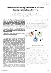
CHAPTER 1 INTRODUCTION Wireless Sensor Networks are a result of the combination of advances made in the field of analog and digital circuitry, wireless communications and sensor technology. A wireless sensor network typically consists of small devices called sensor nodes that are capable of sensing the environment around them. The sensor nodes are devices that are capable of sensing, gathering, storing and transmitting information. The main advantage of these nodes is their self-organizing capability. Large networks of such small nodes are therefore growing in use. The sensor nodes can be deployed anywhere without actually having to install or deploy them manually. In remotely inaccessible areas, these sensor nodes are just strewn across the desired sensor field. The self-organizing capability of the sensor nodes enables the nodes to form a cooperative network and gather information. This information can then be retrieved. Thus, sensor networks enable intelligent monitoring of inaccessible areas with ease and accuracy. Wireless sensor network (WSN) is a term used to describe an emerging class of embedded communication products that provide redundant, fault-tolerant wireless connections between sensors, actuators and controllers [25]. Figure 1.1 shows a wireless sensor network with sensor
Source node
sensor nodes
nodes, a source node and a sink node.
Sink node Figure 1.1 Wireless Sensor Network 11
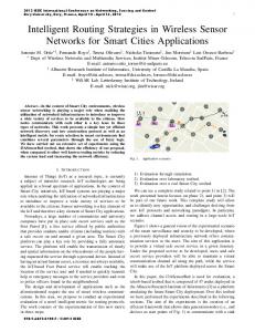
1.1 The Sensor Node Like all other technologies, wireless sensor networks are also subject to constraints. One of the major challenges is the energy constraint of the sensors nodes. Sensor nodes are driven by a battery and have very low energy resources, which in turn affects the network lifetime [26]. Figure 1.2 shows the architecture of a sensor node.
Power Source
Transceiver
Sensor 1
Micro-controller
ADC
Sensor 2 External Memory
Figure 1.2 Architecture of a sensor node 1.1.1 Components of a Sensor Node From the Figure 1.2 [27], the components of a sensor node are a microcontroller, a transceiver, external memory, a power source and sensors. Microcontroller: The microcontroller performs tasks, processes information and controls the functionality of the other components in the node. Microcontrollers are best suited for sensor nodes due to their flexibility to connect to other devices, less power consumption and the fact that the microcontroller can enter a sleep state wherein only a part of the controller is active, thus saving energy.
12
Transceiver: Sensor nodes operate in the Industrial, Scientific and Medical (ISM) band, which provides free radio, huge spectrum allocation and global availability. Radio frequency communication is best suited for sensor networks. Sensor networks use the communication frequencies between 433 MHz and 2.4 GHz. The transceiver provides the functionality of both the transmitter and the receiver in the sensor node. External Memory: Mostly, the on-chip memory of the microcontroller and flash memory are used, and off-chip Random Access Memory (RAM) is barely used. Depending on the type of storage, two kinds of memory are used: user memory for storing application related or personal data, and program memory for programming the device. Power Source: The sensor node consumes power for sensing the environment, gathering information, storing and processing the information gathered. Most of the energy is spent for communication with other nodes in the network and staying active. Batteries are the main source of power for sensor nodes. Sensors: A sensor is a device that responds to a change in its surroundings in a measurable manner. The continuous analog signal that is sensed by the sensors is digitized by analog-to-digital converters and sent to the controllers for further processing. Sensors should be small, adaptive to the environment, operate and configure on their own, and consume low power. There are two types of sensors, active and passive. Active sensors gather data by probing into the environment, while passive sensors gather data without actually disturbing the environment.
13
1.2 Hardware and Software The hardware related to wireless sensor networks is a result of advances in technologies such as system-on-chip technology that is capable of integrating systems on a single chip, commercial Radio-Frequency (RF) circuits that enable short distance wireless communication with low power consumption, and the Micro-Electro-Mechanical Systems (MEMS) technology that integrate sensors onto a single CMOS chip [28]. The first commercial manufacturer of Intel motes was Crossbow Technology Inc. [5]. This was followed by Intel’s Stargate gateway computer network and the Intel r Mote, equipped with 32-bit central processor and Bluetooth wireless standard [5, 31]. The Smart Dust project lead to Spec motes that have reduced large motes into single chips excluding batteries. TinyOS [5, 29], a freely-available open source operating system was developed for MICA2 sensor nodes, and also another programming environment for sensor nodes called EmStar [5, 30] came into existence. NesC is an extension of the C programming language and is used by sensor nodes to communicate between themselves.
1.3 Problem Description and Motivation Sensor networks are easy to deploy and enable us to remotely monitor practically inaccessible areas. One major challenge posed by sensor networks is wasteful usage of resources. Once deployed, sensor nodes are solely battery operated and left to self organize and process information. It therefore becomes very important to keep the nodes up and running for as long as possible. Energy consumption is hence a very serious issue of sensor networks. In [20], network partition is recognized as a major problem in densely populated sensor networks. In [5], network partition is defined as an event when
14
the source node and the sink node are last connected. We therefore define the network as partitioned when no communication link can be established between the source node and the sink node. This loss of communication between the source and the sink nodes is a result of exhausted battery life of the sensor nodes in the network. Hence network partition is directly affected by the energy consumption of the nodes in the network. The motivation of our work is to study network partition and the energy consumption of the wireless sensor network.
1.4 Objectives This work studies the conditions leading to network partition, and analyzes energy consumption to prolong the network lifetime. We focus on implementing routing in densely populated sensor networks. By maintaining constant values for parameters such as path loss exponent, receiver sensitivity and transmit power, and varying between uniform and types of non-uniform grids, we observe energy consumption patterns for each of the grid structures, and infer from the network lifetime the best suited grids for uniformly and randomly deployed sensor nodes. We try to achieve the following objectives: 1. Design non-uniform grid-based coordinated routing. 2. Observe network lifetime for different types of non-uniform grids under different node densities. 3. Extend network lifetime by routing only through grid coordinators. 4. Infer the best suited non-uniform grid structure for prolonged network lifetime.
15
5. Verify the results of the algorithm through simulations, and compare between different simulations.
1.5 Contributions The main contributions of our work are:
Design and implement non-uniform grid-based routing with different types of non-uniform grids.
To maintain load balancing among the sensor nodes.
Determine the best type of grid suitable for uniform and random deployment of nodes, and for different node densities.
1.6 Organization Chapter 2 deals with the different routing protocols used for wireless sensor networks. It discusses the traditional routing protocols, ad-hoc routing protocols and routing protocols developed for wireless sensor networks. Chapter 3 describes the traditional flooding algorithm, and also deals in detail about two routing protocols, namely the Geographic Adaptive Fidelity and Span protocols which are the main idea behind grid-based routing. Chapter 4 presents the grid-based routing protocol, and also explains in detail the nonuniform grid-based routing protocol, including electing coordinators, determining the grid size for the network, and load balancing in our protocol. It also presents the different types of non-uniform grid structures.
16
Chapter 5 presents simulations and results for various non-uniform grid structures, the uniform grid structure and the traditional flooding algorithm. Chapter 6 presents conclusions and future directions for our work. Finally, the source code for all simulations, in Matlab, is provided in the appendix.
17
18
CHAPTER 2 ROUTING PROTOCOLS FOR WIRELESS SENSOR NETWORKS 2.1 Introduction Wireless sensor networks are wireless networks consisting of autonomous sensor nodes, communicating with each other over wireless links. There are basically two modes in wireless networking: infrastructure mode and ad hoc mode. Wireless sensor networks are a form of ad hoc networks. Infrastructure mode requires the use of connecting points, such as access points, to connect a wireless network to a wired network. The additional cost of the equipment is a major drawback of infrastructure networks. Unlike the infrastructure mode, the ad hoc mode supports networking applications when a fixed infrastructure is unavailable. Communication in ad hoc networks does not rely on a central access point or connecting points, but allows wireless devices or nodes to communicate directly to each other. Mobile ad hoc networks are thus self-organized networks where the nodes discover each other and act as routers, maintaining information about their neighbors and themselves. Each node in the ad-hoc network may be the final destination for packets, or may act as a forwarding node or station for transmitting packets to their final destination. Each node in a sensor network consists of a central processing unit, memory, a Radio Frequency (RF) transceiver, and a power source which is usually a battery. The lifetime of the node plays a vital role in supporting network connectivity in ad-hoc networks. Several energy conserving mechanisms have been proposed to extend the lifetime of the network. We will look at some of these schemes in this chapter.
19
2.2 Traditional Routing Protocols An efficient routing protocol will help minimize the load on each individual node, and also minimize the traffic overhead over the network. Traditional routing protocols are aimed at finding optimal routes to every host in the network, and are not suitable for adhoc networks. A mobile ad hoc networking (MANET) working group has been formed within the Internet Engineering Task Force (IETF) to develop a routing framework for IP-based protocols in the ad hoc networks [1]. These ad-hoc routing protocols are divided into table-driven and on-demand protocols. Table-driven routing is also called proactive or precomputed routing, while on-demand routing is called reactive routing. Tabledriven protocols require the use of routing tables at each node to keep track of routes to different nodes and make use of periodic broadcasts for periodic updates. On-demand algorithms do not maintain such routing tables, but use a procedure to identify a route as and when a source requires to transmit information to a destination. Table-driven algorithms can be classified into [1, 2]:
Destination-Sequenced Distance Vector Routing (DSDVR): The DSDVR is a table-driven algorithm based on the classical Bellman-Ford routing mechanism. Each node in the network maintains a routing table, consisting of all the destinations in the network and the number of hops to each destination. Each entry is marked with a sequence number, to distinguish old routes from new routes. Routing table updates can employ two types of packets: full dump, carrying all available routing information, and incremental packets carrying information that has changed since the last full dump. The route with the most recent sequence number is used mostly.
20
Clusterhead Gateway Switch Routing (CGSR): The CGSR protocol uses a cluster head algorithm to determine a node as the clusterhead within a cluster. This protocol uses the DSDVR protocol as its underlying routing scheme, but uses a hierarchical cluster-head-to-gateway routing approach to route packets. On receiving a packet, a node consults its cluster member table and its routing table to determine the next cluster head in the route to the destination.
The Wireless Routing Protocol (WRP): In WRP, each node maintains four tables, namely distance table, routing table, link-cost table, and Message Retransmission List (MRL) table. The MRL table consists of the sequence number of the update message, a retransmission counter, an acknowledgement-required flag vector and a list of updates sent in the update message. Changes in the links are known between nodes through the use of update messages. Neighbors are recognized by the receipt of acknowledgements and other messages. If a node is not sending any messages, to ensure connectivity, it must send a hello message within a specified time. If the node fails to do so, the link fails. New nodes are also required to send hello messages so that they can be added to the node’s routing table.
These protocols are advantageous in the fact that a route is available as and when required, and there is no delay experienced until the route can be determined. However, table-driven algorithms are not suitable for self-configuring mobile ad hoc networks as most of the network capacity is used up in maintaining current routing information.
21
2.3 Ad-hoc Routing Protocols Though conventional protocols are well tested and are quite familiar to use, they pose a major drawback as they are designed for a static topology and hence, are not suitable for constantly changing networks. Conventional protocols like link state and distance vector rely highly on periodic control messages [13]. As the density of ad-hoc networks increases, it becomes difficult to maintain large and frequent exchange of such control messages. Because all such information relies on transmission over the air, maintaining such information for a wireless network implies high cost, usage of bandwidth and battery power. Thus, using traditional protocols for ad-hoc networks would only lead to wastage of resources. Wireless sensor networks, which are a form of wireless ad hoc networks, would therefore require reactive or on-demand protocols. Most of the ad-hoc routing protocols have an underlying traditional protocol algorithm. Ad-hoc routing protocols or reactive protocols can be classified into [1]:
Ad Hoc On-Demand Distance Vector Routing – This protocol has been classified as a pure on-demand route acquisition system. In this mechanism, if a node requires to transmit a packet to a node that does not already have a route to it, the node initiates a path discover process to locate the destination node, by broadcasting a route request packet to its neighbors. The neighbors in turn, broadcast the packet to their neighbors, and this continues till the route to the destination is discovered. Each node maintains its own sequence number, and a broadcast identity (ID), which is incremented for every route request packet the node initiates. Intermediary nodes that receive the request packet record the
22
address of the neighbor the packet arrives from, and discard any additional requests received from these neighbors. When the request reaches the destination, the node responds by unicasting a route reply packet back to the neighbor it receives the request from.
Dynamic Source Routing (DSR): The DSR protocol consists of two main phases: route discovery and route maintenance. When no route exists to a destination, the route discovery process is initiated by broadcasting a route request packet. Each node that receives the packet checks to see if it can locate a route to the destination, and if not, adds its address to the route record of the packet, and then forwards it. A route reply arrives when the request reaches the destination. Route maintenance makes use of route error packets and acknowledgements.
Temporally Ordered Routing Algorithm (TORA): This algorithm is a highly adaptive loop-free distributed routing algorithm, based on link reversal. The key concept of this algorithm is the localization of control messages to a small set of nodes. This protocol performs three basic functions – route creation, route maintenance, and route erasure.
Associativity-Based Routing – The Associativity-Based Routing protocol defines a new routing metric, known as the degree of association stability, based on which a route is selected. Each node signifies its existence by generating a beacon periodically and upon its reception by the neighboring nodes, their associativity tables are updated. The three phases of this algorithm are: route discovery, route reconstruction and route deletion.
23
Signal Stability Routing: This protocol selects routes based on the signal strength between the nodes and a node’s location stability. This can be further classified into two protocols: the Dynamic Routing Protocol (DRP) and the Static Routing Protocol (SRP). The DRP maintains the signal stability table and the routing table while the SRP processes packets.
Table-driven routing protocols rely on the information contained in the routing table, continuously updating the routing table. This is not the case with on-demand routing protocols, where a node has to wait to discover a route to a destination. Though tabledriven protocols have a route available even before it is needed by a node, they are not suitable for reconfigurable ad hoc networks. On-demand routing protocols are better for self configuring mobile wireless sensor networks.
2.4 Related work In response to the needs of wireless sensor networks, new protocols have been proposed to meet the requirements of wireless sensor networks. A few of these are listed below:
Flooding: Flooding is a technique where each node receives a packet which it broadcasts to its neighbors, which in turn broadcast to their neighbors. This process continues till the maximum number of hops has been reached for the packet, or the destination has been reached [3].
Gossiping: Gossiping is different from flooding in the way that the nodes do not broadcast to all their neighbors, but randomly pick a neighbor and then forward the packet to it. Each node then again picks a random neighbor and transmits the packet to it. 24
Sensor Protocols for Information via Negotiation (SPIN) [4, 16]: SPIN uses a data-centric routing mechanism, and names the data using meta-data that describes the characteristics of that data. There are three types of messages in SPIN, namely ADV, REQ and DATA. ADV is used for advertizing that a node has data to send, REQ is when a node is ready to receive data and DATA contains the actual data. SPIN solves the problems of flooding and is very energy efficient, but is not scalable, and due to its data advertisement mechanism, the life time of a node is affected.
Directed Diffusion [4, 14]: This algorithm uses a naming scheme for the data to transmit data through the nodes. The sink node sends out task descriptors to all the nodes, called the interest. The interest and data propagation and aggregation are determined locally. The main advantage of this scheme is that it saves energy, but results in overhead and synchronization problems in the network.
Low Energy Adaptive Clustering Hierarchy (LEACH) [4, 15]: LEACH is a clustering based protocol, wherein clusters are formed based on the received signal strength, and clusterheads are used to route packets between these clusters. These clusterheads are changed randomly to distribute the load equally on all the nodes. LEACH adopts direct hop transmission instead of multi-hop transmission, but the main drawback is the fact that this algorithm was designed taking into consideration assumptions that do not actually refer to the wireless sensor network architecture.
Power-Efficient Gathering in Sensor Information Systems (PEGASIS): PEGASIS relies on LEACH, and is a chain-based power efficient protocol. The chain can be
25
constructed using a greedy algorithm, since all nodes have global network information. This algorithm suffers from the problem of scalability and keeping global information about the network.
Geographic and Energy Aware Routing (GEAR): As the name suggests, GEAR uses energy aware and geographically informed neighbor selection to transmit the packets to their destination.
Energy efficiency is a key challenge in wireless sensor networks, and energy consumption is dominated by the energy required to keep the nodes active and running. Many topology management schemes have been proposed so as to cleverly choose nodes to be put to sleep without affecting the capacity of the network. We will focus more on these schemes here:
Geographic Adaptive Fidelity (GAF) [18]: GAF uses the fact that neighboring nodes can replace each other in the routing topology. The sensor network is divided into small grids, and nodes in the same grid are equivalent in routing. At a point of time, only one node is active in each grid, while the other nodes in the grid can stay in the energy saving mode. This algorithm is very helpful in the case of dense networks.
Span [17]: In Span, the capacity of the ad hoc network is conserved by a set of nodes that forms a multi-hop forwarding backbone. Nodes other than the nodes in this set transition to sleep states frequently. The functionality in the backbone network is rotated through the set of nodes to distribute load equally.
Sparse Topology and Energy Management (STEM) [19]: STEM is a topology management technique that emulates a paging channel by having a separate radio
26
operating at a lower duty cycle. When a wakeup message arrives, the primary radio is turned on, and this takes care of the data transmissions. STEM can integrate with the above two schemes to produce energy savings beyond GAF or Span alone.
Adaptive Self-Configuring sEnsor Networks Topologies (ASCENT) [20]: Each node in the network assesses its connectivity and adapts its participation in routing. Initially, a few nodes are active while other nodes are only listening and not transmitting. Help messages are sent to listening nodes to join in the network, and become active neighbors. This continues till the number of active nodes reaches a certain value. When this is done, the data delivery is more reliable since there are more active nodes participating in the routing process. The process of inviting more neighbors to join in the network starts again when a network event or change triggers the need for more active nodes in the routing path.
Cluster-based Energy Conservation (CEC) [21]: CEC creates clusters, selecting clusterheads based on the highest remaining energy that is advertised.
Adaptive Fidelity Energy-Conserving Algorithm (AFECA) [21]: AFECA allows each node to sleep for the number of neighbors it has. Therefore if a node has a large number of neighboring nodes, it can sleep longer without affecting network connectivity.
Several topologies have been proposed for conserving energy in sensor networks including cluster, link, grid, and diffusion, which were adopted to route packets across the sensor network. Amongst these, the grid-based approach, as put forward in the GAF
27
algorithm is more suited for sensor networks, since the grid topology can dynamically be configured with the configuration of the nodes. In [5], the authors explore grid-based coordinated routing in wireless sensor networks. The underlying routing protocol is based on flooding, but unlike flooding, grid-based coordinated routing reaches only selected nodes in the field. Sensor nodes are randomly deployed over a sensor field, and the entire field is divided into square shaped grids, of sizes defined by the user. Of the nodes in each grid, one node is elected as the coordinator node, which actually takes part in the routing process while the remnant nodes power down their radios to save energy. The source floods the network with a query message to each coordinator. When the message reaches the sink node, the sink node sends information by tracing a route back to the source node. This process continues till a coordinator node in the route runs out of energy. Nodes in the network are assigned ID’s. Coordinator nodes are elected based on the ID’s. The node with the highest ID in the grid is elected to be the coordinator. If this node runs out of energy, the next highest node is elected as coordinator. New coordinators are elected to replace nodes that run out of energy. The process continues till the network is partitioned and the connection between the source and sink is lost. This scheme employs load balancing to keep the nodes running for a long time. In [6], a directed grid topology is proposed from the source node to the sink node. This grid is constructed with respect to the diagonal line between the source and sink nodes. Here, the sink node can move around in the network and hence the topology of the grid varies according to the positions of the source and sink nodes. The parameter determining the distance between the grids is the average transmission cost, unlike in the previous
28
scheme. There are two criteria for selecting a grid node: the distance to the location of the ideal grid node and the residual power. A cost parameter has been defined as the metric to select a grid node. The next hop is determined by the node with the smallest value for the cost parameter. There are two contributions of this scheme, namely the optimal grid distance is derived from the from the transmission cost point of view. Also, the routing scheme can be used for one sink and single or multiple sources. In [7], the concept of grid-based routing is proposed wherein variants of grid-based routing are proposed for different environments. The authors maintain that grid-based routing requires as few grids as possible to participate while ensuring network connectivity. The notion that to keep the network connected one node per grid is required to stay active is contradicted with the argument that a largely reduced subset of grids can still preserve the same degree of coverage. This paper therefore puts forward variants of grid-based routing schemes which reduce the number of grids that are required to support routing while supporting network connectivity. Also, the authors demonstrate that diagonal routing with a different side length of grids outperforms rectilinear routing. The above mentioned grid-based schemes are common with the fact that they propose routing schemes for a uniform grid structure. In [8], a non-uniform grid structure is proposed for the GAF protocol, by deducing the relationship between the optimal radio range and traffic in the network. The minimum energy consumption characteristic range is not a constant but varies with the amount of traffic. Optimal range increases as the loaded traffic decreases. To save energy by radio range adjustment, the network is divided into sections of different sizes, according to a derived range-traffic relationship. The number of grid sections is not a free parameter as in the case of the GAF protocol.
29
The authors demonstrate that a lower energy consumption is achieved by the non-uniform virtual grid routing, as compared to the values for the uniform grid.
2.5 Conclusions Presented in this chapter are the different routing protocols for wireless sensor networks and different topology management schemes in use. Amongst all the topology schemes proposed, grid-based topology management is more affective in terms of energy efficiency and extending network lifetime. Grid-based schemes can be of a uniform grid structure and a non-uniform grid structure. Uniform grid-based routing can be modified to fit in different environments. Between the two of them, non-uniform grid-based routing is more energy efficient than uniform grid-based routing.
30
CHAPTER 3 FLOODING, GAF AND SPAN 3.1 The Flooding Algorithm The flooding algorithm is one of the most simple and widely used algorithms in a pointto-point communication network. In the flooding algorithm, the source first broadcasts information to all its neighboring nodes. Each receiving node, in turn broadcasts the information it receives to all its neighboring nodes, other than the source node. The information thus traverses from the source node to the destination node and through all the nodes in the network. The basic algorithm for flooding is as shown below: Algorithm 1: For the source , do: Send the message on all outgoing links. For vertex do: If the message is received for the first time: 1. Store the information in an output buffer. 2. Forward the message to every other node in its own vicinity. If the message is received again, discard the message. End Though flooding algorithm is easy to implement, it is still complex and poses its own challenges. Flooding is inefficient in terms of network bandwidth utilization, because each node transmits and receives multiple packets of data, thus wasting network bandwidth. Real world flooding is considerably complex as care has to be taken to avoid duplication of data packets, infinite loops and clearing the output buffers of multiple entries of data.
31
Figure 3.1 Simulation topology showing the traditional flooding algorithm. Another flooding algorithm that shows a flooding-based tree construction protocol for avoiding duplicate deliveries [5] is as shown below: Algorithm 2: FLOOD (Node S) if Node n receives the packet for the first time then Mark Node n as received Parent ⇐ S Source ⇐ n Increment Level Field Rebroadcast packet end if In this algorithm, the node which sends the packet to a node for the first time is the parent of the node. The Level field is incremented by one, and then the packet is rebroadcast.
32
The Level field is to denote the number of hops the node is away from the source node. The main advantage of this flooding is that a node can receive a packet only if it has not yet received a packet. Therefore, the duplication of data packets is reduced and hence the network bandwidth is efficiently utilized to a certain extent. Every node in this algorithm has a unique parent and as many children as the nodes it can reach. This flooding algorithm is an improvisation of the traditional flooding algorithm.
3.2 Motivation A wireless sensor network is a wireless network of spatially distributed sensors, which respond to any change in the physical or environmental conditions. The sensor node gathers information by responding to changes in its surroundings, processes the information so gathered and communicates the same with its neighbors. Power consumption is a very important issue for deploying wireless sensor networks as each node operates with limited power and the lifetime of the nodes effects the lifetime of the wireless sensor network. If each node was to transmit directly to its destination, the amount of power it consumes for each transmission would deprive the node of its energy completely. Hence direct transmission is beneficial when the destination is within a limited coverage area. Transmitting packets in a multi-hop manner, wherein the consumption of power can be shared by all the nodes in the network increases the network lifetime. Each node controls its transmission power and self organizes a network topology by controlling its coverage area. The network topology can therefore be dynamically changed, in accordance with the neighboring nodes. In multi-hop transmission, selection of the intermediate node is
33
done considering not only the shortest path possible but also by taking into account the residual power of the potential intermediary nodes. This is important because selecting the same intermediate nodes often will result in depleting the intermediate nodes of their energy, and causing the nodes to die. This will in turn decrease the network lifetime. Therefore, focusing on network longevity, many topologies have been developed to route packets from the source node to the destination node. The various topologies adopted for routing packets in sensor networks are grid, cluster, link, and diffusion topologies. Amongst them, the grid approach is most beneficial, since the topology of the grid can be configured dynamically with respect to the source and the sink nodes, and also there are multiple paths between the source and the destination, making the selection of the forwarding path and the intermediate nodes flexible. The grid approach was designed to achieve node equivalence in a network, and was implemented initially in the GAF and SPAN protocols [6].
3.3 Geographic Adaptive Fidelity The GAF [9] protocol belongs to the class of protocols that concentrate on energy consumption to increase network lifetime. The energy consumed by sensor nodes for transmitting, receiving and idle listening is significant and is wasted. When significant node redundancy exists in the ad hoc network, it is observed that intermediary nodes can actually be put to sleep, or turned off to conserve energy while still maintaining the connectivity of the network. Routing fidelity, defined as the uninterrupted connectivity between communicating nodes, can be maintained as long as any intermediate node is
34
awake. In GAF, routing fidelity is maintained to be constant while node behavior is adapted to extend network lifetime. GAF uses a virtual grid over the entire sensor field, and each node associates itself with this virtual grid. Node location in GAF is determined by using Global Positioning System (GPS) or other location systems. All nodes in a particular grid are equivalent with respect to forwarding packets. In each grid, nodes determine which of them will sleep and for how long, and which node will remain active for a certain period of time. To balance the load in the network, sleeping nodes turn on their radios periodically and trade places with the active nodes, which then turn off their radios. The distance between any two nodes is within the nominal radio range of the nodes, to maintain connectivity in the network. Each node in GAF has three states: sleeping, discovery and active states respectively. Nodes are initially in the discovery state, when they send and receive discovery messages to find other nodes in the grid. In the discovery state, the node sets a timer, after which it broadcasts its discovery message and enters the active state. In the active state, the node again sets a timer for how long it will stay active. Once this timer expires, the node enters into sleeping state and lets other active nodes handle routing for that grid. Nodes in each grid are ranked according to their remaining energy level. GAF employs load balancing using node ranking to maintain the nodes running for as long as possible, thereby increasing network lifetime.
3.4 SPAN Span [10] is a technique that is similar to GAF algorithm with regard to power conservation in sensor nodes. Unlike GAF, Span does not divide the entire network into 35
grids, but instead it elects coordinator nodes from all the nodes in the network to participate in routing. Span thus forms a backbone network of active nodes that participate in the actual routing while the other nodes in the network, that are not part of this backbone network turn off their radios to conserve energy. Load balancing is achieved by rotating the role of the coordinator node amongst all the nodes in the network. Span does not require knowledge about the location of the nodes to elect coordinates, but uses local information to know about neighboring nodes and elect coordinators. Coordinators are elected such that every node is in the radio range of a coordinator node. These coordinators actively participate in routing while the other nodes in power saving mode periodically check to see if they should wake up to act as coordinators and participate in routing. The Span protocol operates under the routing layer, and above the medium access layer. Each node in Span broadcasts HELLO messages that contain the node’s status, its current coordinators and its neighbors. At a time, only those entries in the routing table that correspond to current coordinators are used for routing packets to and from the destination node. Unlike GAF, a node in Span can only be in two states: coordinator and a non-coordinator. A node volunteers to be the coordinator if two of its neighbors fail to communicate with each other, either directly or through another coordinator. In other words, a node offers itself to participate in routing if it can detect loss of connectivity among the neighbor nodes. A node determines whether to participate in routing by considering two factors: the energy remaining in the node and the number of neighbors it can connect by using up its battery life. This ensures that maximum connectivity is
36
achieved with the least possible number of active nodes, thus maintaining network longevity.
CHAPTER 4 UNIFORM AND NON UNIFORM GRID BASED ROUTING 4.1 Grid-based Coordinated Routing The main focus of Grid Based Coordinated Routing (GBCR) is on partitioning the network into square shaped grids to extend network lifetime. The entire network is divided into equally shaped grids, and in each grid an active node, the coordinator is elected, like in the Span algorithm. The underlying routing algorithm used in GBCR is similar to level flooding. The following algorithm is used by grid-based coordinated routing protocol [5]: Algorithm 3 Grid-based coordinated routing protocol C ⇐ set of coordinator nodes while network is not partitioned do while C ≠ Ø or sink node not yet reached do Pick a node randomly from C FLOOD( ) end while send information from the sink node back to the source node elect new coordinator nodes C⇐ In grid-based coordinated routing, information reaches only selected nodes in the field instead of to all the nodes in the network. The main idea of dividing the network into grids is to make only one node alive for each grid, while the rest of the nodes in that grid are sleeping so as to conserve their battery life. In each grid, the coordinator participates 37
in routing as long as the amount of energy in that coordinator is above a certain threshold value. When the energy drops below the threshold, a new coordinator is elected for that grid. The source transmits information to the sink through the active coordinators, and the sink traces a route back to the source. The process of flooding continues till the nodes participating in the routing run out of energy, when new coordinators are elected and a new route back to the source from the sink is calculated. The source starts flooding by sending a query message to all the neighbor coordinators, which flood other coordinators in the network till the message reaches the sink node. Each coordinator node in grid-based routing has three states, namely, routing, warning and depleted states. When coordinator nodes in a particular route die, or run out of energy, new coordinators are elected to replace the old nodes. All nodes in the network are randomly assigned IDs. In each grid, the node with the highest ID becomes the coordinator. When the node with the highest ID runs out of energy, the node with the next highest ID becomes the coordinator for that grid. Each time the coordinator node changes the sink node traces back a route to the source node.
38
Figure 4.1The uniform grid structure of grid-based coordinated routing protocol.
39
Figure 4.2 The uniform grid structure with 100 sensor nodes deployed uniformly in the field. Grid-based coordinated routing adopts a grid structure as shown in Figure 4.1. Each grid is a square of side of a fixed length, 200 m for example. Different results have been observed by varying the grid size from 50 m to 200 m. Connectivity in the network depends on the grid size, transmission range and the sensitivity of the nodes. When grid coordinators are elected, care should be taken such that the coordinators must still be able to connect to neighboring grid coordinators. Therefore, grid size is very important to maintain connectivity throughout the network as too large a grid size will result in loss of connectivity of the nodes in the network. Grid-based coordinated routing places an upper bound on the grid size and determines the conditions to maintain connectivity throughout the network depending on the grid side and the transmission range of the nodes. Grid-based coordinated routing maintains load balancing as does Geographic Adaptive Fidelity. The function of the coordinator node is distributed amongst the nodes in the network based on the ranking of the nodes in each grid. GBCR observes the effects of transmit power, receiver sensitivity and grid size on network lifetime, and determines that decreasing the transmit power increases network lifetime. 4.2 Non Uniform Grid-based Coordinated Routing Excluding some of the nodes in the network to participate in routing to conserve battery life and increase network lifetime was proposed in SPAN. The idea of a virtual grid over the network field was proposed in the Geographic Adaptive Fidelity algorithm. Dividing the entire network into equal sized grids, and electing nodes in each grid to participate in routing while other nodes were put to sleep was introduced in grid-based coordinated
40
routing. Uniform grid-based routing is efficient when the distribution of the nodes in the sensor field is uniform. Varying the grid sizes in the network extends the lifetime of the network. In [8], the relation between optimal radio range and traffic is used to define a non-uniform grid for the GAF protocol. In this work, we apply the non-uniform grid size for the grid-based coordinated routing protocol and analyze the results of the same. 4.3 Non-uniform grid-based routing protocol The underlying routing algorithm of non-uniform grid-based routing protocol is the same as the grid-based coordinated routing protocol. The entire sensor field is divided into nonuniform sized grids. In our work, we consider three different non-uniform grids. Figures 4.3 to 4.5 show the different types of grid structures we consider for simulation.
41
Figure 4.3 Topology showing the alternating non-uniform grid structure called the alternate structure with 100 nodes uniformly deployed across the field and alternate small grids of 100 m each side, and large grids of 200 m each side. In each grid, as in the uniform grid-based routing, from all the nodes of the grid, a coordinator node is elected that involves in the routing process, while the other nodes in the grid save their battery by putting themselves to sleep. New coordinators are elected when the node runs out of energy or falls below a threshold value.
Figure 4.4 Simulation topology showing the source non-uniform structure with 100 sensor nodes deployed uniformly in the field wherein the area containing the source node is divided into small grid sizes of 100 m each, while at the sink node the area is divided into grids of size 200 m each. Though the grid sizes can be varied, we fix the lower bound on the grid size to be 100 m and the upper bound as 200 m. Also, we do not take into consideration the other possible non-uniform grid structures, as the results show no significant improvement for the same. 42
Figure 4.5 Simulation topology showing the sink non-uniform grid structure with 100 nodes deployed uniformly across the field, wherein the vicinity around the source node is divided into 200 m sized grids while the area in the vicinity of the sink node is divided into 100 m sized grids. 4.4 The Link Models For successful transmission between two nodes, a successful link has to be established. A major challenge to wireless networks is the lossy nature of the wireless links. There are many link models that exhibit the lossy nature of wireless links, but for wireless sensor network, we consider the deterministic link model and the probabilistic link model. 43
4.4.1 Deterministic Link Model The amount of energy that is required to establish a link between two nodes is proportional to the distance between the two nodes raised to a constant power, called the path loss exponent, n [11]. For the deterministic link model, the value of the path loss exponent is usually assumed to be between 2 and 4. This is represented in the following equation: =
/
;
(1)
where is the power of the received signal; is the transmit power; d is the distance between the two nodes and n is the path loss exponent. If S is the receiver sensitivity, the communication link between the two nodes leads to a successful transmission between the nodes if
is greater than S.
4.4.2 The Probabilistic Link Model Results from [12] show that for a given power setting, there is a region within which all the nodes have good connectivity, called the effective region and a distance beyond which the nodes show poor connectivity. The size of the effective region is observed to increase with transmit power. Between the two extreme points lies the transitional region, where the average link quality drops off smoothly.
44
Reception Success
100%
0% A
B Distance
Figure 4.6 Probabilistic link model. The deterministic link model does not take into account multi-path fading, which either increases or decreases the possibility of a successful communication link. This is included in the current model by a random number R, as shown below [5]: =( /
∗R
(2)
If nodes within the point A are guaranteed to successfully receive a transmission, and nodes beyond a point B are guaranteed not to receive a transmission, then the nodes between the points A and B are the nodes that are affected by the multi-path variation. From [5], the probability of transmission between the points A and B is determined by the equation as shown: R= where
+ (1− =
) ∗ rand(1) ∗ S)/
(3)
, and
(4)
rand(1) is a random number uniformly distributed between 0 and 1.
45
To calculate the power of the received signal, the value of R is substituted in (2). Thus when the distance between the two points A and B is known, the transmission success of a packet is determined probabilistically. 4.5 Determining the grid size To ensure connectivity between any two coordinator nodes in adjacent grids, proper grid size must be determined. Grid size is affected by factors such as the transmission range of the transmitter, or the transmission power and the sensitivity of the nodes. If the grid size is too large, it will lead to early partition of the network if the coordinator nodes are located too far off from each other. Thus, it cannot form a link between the nodes even if the nodes are alive in each grid. From (1), d is the maximum distance for successful transmission, when S. If this maximum distance is
, then
is the nominal radio range,
defines a virtual grid as follows [9]:
r
2r FIGURE 4.5. Determining the
2r The maximum limit for the side r can be estimated as follows:
46
is set equal to . GAF