Indeed black holes evaporate via Hawking radiation and even- tually disappear. ... We describe a simple model of non unitary effects where some probability.
Discrete Mathematics and Theoretical Computer Science
DMTCS vol. 12:2, 2010, 333–362
Non Unitary Random Walks Philippe Jacquet INRIA, Le Chesnay, France
received July 30, 2009, revised Apr 19, 2010, accepted May 5, 2010. Motivated by the recent refutation of information loss paradox in black hole by Hawking, we investigate the new concept of non unitary random walks. In a non unitary random walk, we consider that the state s0 , called the black hole, has a probability weight that decays exponentially in e−λt for some λ > 0. This decaying probabilities affect the probability weight of the other states, so that the the apparent transition probabilities are affected by a repulsion factor that depends on the factors λ and black hole lifetime t. If λ is large enough, then the resulting transition probabilities correspond to a neutral random walk. We generalize to non unitary gravitational walks where the transition probabilities are function of the distance to the black hole. We show the surprising result that the black hole remains attractive below a certain distance and becomes repulsive with an exactly reversed random walk beyond this distance. This effect has interesting analogy with the so-called dark energy effect in astrophysics. Keywords: random walks, quantum systems, analysis of algorithms, generating function, continuous fractions, singularity analysis
1
Introduction and motivation
A black hole is a massive stellar object that absorbs everything that get trapped in its gravitational field, including light. In 1976, the famous astrophysicist Stephen Hawking [2], predicted that the black holes cannot be absolutely black and eternal. Indeed black holes evaporate via Hawking radiation and eventually disappear. A major problem was detected in the fact that Hawking radiation should not carry any information and therefore the informations contained in the objects absorbed by the black hole during its lifetime simply disappear. This information loss paradox leads to fundamental question in theoretical physics since it apparently violates the principle of unitarity in quantum physics (more details are given in our Section 2). There are many studies related to the question of non unitary quantum gravity. Some of these studies has given the opportunity of numerical simulations of non trivial complex systems [8]. In 2006 Hawking [11] refuted his original argument about the information loss paradox. His refutation is still an object of controversy but established the foundation of non unitary Markov systems. Basically Hawking stated in his 2006 paper that if black holes would host a superposition of unitary and non unitary metrics, then the the contributions of non unitary metric would vanish exponentially with time, and therefore only the effect in unitary metric would remain at infinity. In other words a black hole tends almost surely to be unitary and thus to release its information without loss during its lifetime. The motivation of this paper is to help in some of the computational aspects in the analysis of non unitary Markov systems. We describe a simple model of non unitary effects where some probability c 2010 Discrete Mathematics and Theoretical Computer Science (DMTCS), Nancy, France 1365–8050
334
Philippe Jacquet
weights decay exponentially with time. What is interesting is the effect of the unitary loss on a halo of matter that surrounds a black hole. The matter acts like a gas where particles collide at random times like in a random walk. In physics, random walk problems are investigated via finite element simulations where particles travel between finite boxes of space. Each box is a state in the random walk. In a non unitary random walk, we consider that the state s0 , called the black hole state, is an absorbing state and has a probability weight that decays exponentially in e−λt for some λ > 0. We will show that such non unitary random walks show a behavior which is very sensitive to their tuning parameters, and thus the simulation must be done in the most realistic situation. In this case as in most simulation of large systems in astrophysics we hit some computational boundaries even when using the most powerful super-computers [10]. Indeed, the number of states in a realistic random walk in a galactic halo may exceed 1020 , even after merging a majority of states due to the spherical symmetry. This makes the simulation very hard to process. Furthermore, as we will show later, the impact of the unitarity effect stands in the future of the particle, namely in the quantity of probability weight it will lose after eventually being ingested by the black hole. Therefore the simulations must compute the probability weight of all potential trajectories in the future. In a (classic) unitary universe, all these trajectories sums to one. But in a non unitary universe this is not the case, and computation must involve all possible trajectories, at least within the whole life time of the black hole. A super-massive black hole, like the black hole which lies in the center of our galaxy, has a lifetime of order 1090 years. Such simulation is rather impossible to make: either we have to iterate on a vector of 1020 coefficients over 1090 steps, or we iterate during log2 1090 steps, on the successive squares of the non unitary matrix, which is of size 1020 × 1020 . The object of this paper is to analytically guess the results of such simulations by investigating the asymptotics of non unitary random walks. We show the surprising result that the black hole remains attractive below a certain distance and becomes repulsive or at least neutral beyond this distance. This effect shows an interesting analogy with so-called dark energy effect in astrophysics. One should not confuse the methodology introduced in this paper with the beautiful analyses in [6, 12] where the particular nature of the quantum random walk is contained in the state superposition in the wave function. Here we analysis the random walks in a more classic way without state superposition, the quantum non unitary effect being contained in the unique black hole absorbing state of the random walk. We base our analysis on the framework of many previous fundamental works, i.e. the representation of generating functions of random walks as continuous fractions in [1], the enumeration of paths in random walks in [7], the singularity analysis in the generating functions in [3]. Our work comes in parallel of related works on the use of combinatorics and generating functions on random walks [4, 9], The paper is organized as follow. • In the two next Sections 2 and 3 we describe non unitary effects and analyse a simple model of non unitary Markov system, with only two states. • In Section 3, we extend the analysis over the non unitary Markov systems that contains an infinite number of states, so-called non unitary random walks. We first investigate the impact of non unitary effect on uniform random walks. • In Section 4 we investigate the case of non uniform random walks, so-called concave random walks. To this end we make use of continued fraction generating function representation and show asymptotic results about their behavior around main singularities. We show that under some circonstance,
Non Unitary Random Walks
335
the non unitarity effect of the black hole makes the random walk apparently bimodal, being apparently attractive below a certain state and repulsive beyond that state. • We finish our paper on the special case of gravitational walks (Section 5) and briefly discuss some physical considerations (Section 6), that is the consequence of the bimodal behavior we have found.
2
¨ Non Unitary effect and the Schrodinger’s rabbit
In a classic unitary universe all probabilities sum to one. If you take a rabbit at time t = 0 then one month later the rabbit will be either alive with probability α > 0 or dead with probability β > R0 and α + β = 1. But in quantum physics the sum of all probabilities is interpreted as being the integral |Ψ|2 of the wave function Ψ of the universe. Therefore the sum of probabilities being equal to one is a R no more 2 mathematical statement but a physical statement. Unitarity principle states that for all time t: |Ψ| = 1. R But in a non unitary universe we may have |Ψ|2 6= 1. The loss of information implies a non unitary universe. Hawking describes metrics pertinent for black holes (so-called anti-de-Sitter metrics) where R |Ψ|2 = e−λt for some λ > 0. In other words let assume a rabbit which at time t = 0 is either (with probability α in state s0 inside a black hole embedded with a non unitary metric, or (with probability β) in state s1 outside a black hole in an unitary metric. If the black hole lifetime is t then at time t the probability sum of state s0 will be r0 (t) = e−λt while the probability sum of state s1 will remain at r1 (t) = 1. Consequently the sum of probabilities of the rabbit equals αr0 (t) + βr1 (t) 6= 1 and when t αr0 (t) tends to 0. In other words the rabbit increases the apparent probability of state s0 defined as αr0 (t)+βr 1 (t) never falls in the black hole and stays outside. This is equivalent in finance, to saying that an investor with one euro at time t = 0 puts α cents in a black hole market, and keeps β cents in his pocket. If the black hole market looses value at rate −λ, then at the end of day the investor will have most of his remaining fortune in his pocket. In fact Hawking’s point is not as trivial as exposed above: he does not consider a rabbit, but the whole black hole and considers that its quantum state is a superposition of unitary and non unitary metrics. He shows that on the path integral over the black hole lifetime, the contributions of non unitary metric vanish exponentially, so that only the unitary metric contributions remain. In the following we are not considering state superposition, we assume that either the rabbit is inside the black hole (state s0 ) or far away outside the black hole (state s1 ). This hypothesis is realistic since the two possible space locations of the rabbit are so far apart that quantum state overlaps are negligible. Therefore we treat the problem in a classical way. We can see the rabbit as a classical equivalent of Schr¨odinger cat in an non unitary universe. The original Schr¨odinger cat can be in the superposition of two states s0 and s1 (for instance dead or alive). We introduce the Schr¨odinger rabbit which is either in state s0 or in state s1 , but the probability sum of state s0 decays exponentially with time.
3 3.1
Modelling non unitary systems Non unitary Markov processes
We still consider a two state process with a state s0 and a state s1 (see Figure 1). The state s0 is an absorbing state that mimics a black hole (BH) and during the black hole lifetime the probability sum decays with rate −λ. We consider that the time is discretized and during the black hole lifetime, at each time unit the rabbit has a probability q to fall into the black hole, and therefore a probability p to remain
336
Philippe Jacquet
p p. The objective is to estimate the apparent attraction of the black hole, or more precisely, the apparent repulsion defined below. We call the quantity p˜(t) = p r1r(t−1) , the apparent repulsion probability, and q˜(t) = 1 − p˜(t) = 1 (t) q r0r(t−1) , the apparent attraction probability. The apparent attraction is equal to the attraction probability 1 (t) multiplied by a factor that takes into account the probability decay that the rabbit will experience inside the black hole until the end of the black hole lifetime t − 1, if it falls inside the black hole during this time slot. Starting from the final probability weight [r0 (0), r1 (0)] = [1, 1] (the black hole system returns to unitarity at the end of black hole lifetie), we have [r0 (t), r1 (t)] = [1, 1]Rt . We prove the following very simple theorem whose main purpose is to introduce our methodology
(3)
337
Non Unitary Random Walks
p
ρ BH
€
q
p
p
p
p …
q
q
q
q
q
Fig. 2: Non unitary uniform random walk.
Theorem 1 We consider a two-state non unitary Markov model of black hole with state s0 and state s1 . The state s0 is the absorbing black hole state and quantity ρ > 0 is the probability decay factor on the black hole state. The integer t is the remaining black hole lifetime. Quantity p is the repulsion probability defined as the probability that the rabbit stays on state s1 during an unit step time. When the probability decay factor is greater than the repulsion probability p, then the black hole is apparently attractive when t → ∞, otherwise when ρ ≤ p, the black hole is apparently repulsive when t → ∞. Proof: We consider the case where ρ 6= p. From the fact that the probability sum of state s1 satisfies the t t p p t −pt + pt , we get the apparent repulsion probability p˜(t) = p/r−(p/r) identity r1 (t) = q ρρ−p 1−(p/r)t = ρ + O(( ρ ) ) when ρ > p. In this case the attraction is stronger than the non unitary effect and the rabbit eventually falls in the black hole which exerts an apparent attraction probability q˜(t) = 1 − ρp + o(t) which remains away from zero when t → ∞. In otherQ words the apparent probability that the rabbit will eventually fall t in the black hole which is equal to 1 − k=0 p˜(k), tends to 1 when t → ∞. In the opposite case, when ρ < p, we have p˜(t) = 1 + O(( ρp )t ), the non unitary effect is stronger than the attraction and the black hole is apparently fully repulsive. In other words, the apparent probability Qt that the rabbit will fall in the black hole during this time slot is zero. Moreover, since k=0 p˜(k) remains away from zero when t → ∞, there will be a non zero asymptotic apparent probability that the rabbit never falls in the black hole during the black hole lifetime. When p = ρ, we get r1 (t) = tqpt−1 + pt and p˜(t) = 1 + O( 1t ). Thus the rabbit as an apparent Qt probability not to fall in the black hole during this time slot when t → ∞. But since limt→∞ k=0 p˜(k) = 0, the rabbit has an asymptotic apparent probability 1 to fall in the black hole during the black hole lifetime. 2
3.2
Non unitary random walks
In this section we investigate non unitary Markov systems with an infinite number of states. There is a specific state, the absorbing black hole state s0 and there is an infinite sequence of states s1 , s2 , . . . , sn , . . .. If the rabbit is in state s0 its stay there for the remaining black hole lifetime, if the rabbit is in any of the states sn , for n > 0, then at the time unit it has probability q to shift down to state sn−1 , and probability p to shift up to state sn+1 (see Figure 2). This is a nearest neighbor random walk in one dimension. We denote rn (t) the probabilityP sum when the rabbit is on state sn when the black hole has a remaining t lifetime t. We denote Rn (u) = t≥0 rn (t)u the generating function of the probability sum over all lifetimes t. Let tn the time to black hole from state sn , i.e. the time at which the rabbit hits the black hole when starting its journey at state sn at time 0. The quantity tn is a random variable. Assuming the initial black hole lifetime t, when the rabbit enters the black hole it will experience a probability decay ρt−tn , if tn ≤ t,
338
Philippe Jacquet
otherwise it has no probability decay since we assume P that the black hole loses its non unitarity properties after its evaporation. Therefore we have rn (t) = θ≤t P (tn = θ)ρt−θ + P (tn > t), and thus Rn (u) = Fn (u)
1 1 + (1 − Fn (u)) , 1 − ρu 1−u
(4)
with Fn (u) the probability generating function of tn . Fn (u) satisfies Fn (u) = quFn−1 (u) + puFn+1 (u), and therefore Fn (u) = (F (u))n , with 1 = Fqu (u) + puF (u), which leads to F (u) =
1−
p
1 − 4pqu2 . 2up
(5)
This clearly mimics the fact that such walks can be seen as the product of n consecutive Dyck paths, (reverse the time and cut on the last time the walk reach state sn , for any n > 1). Our aim is to evaluate (t−1) . Cauchy’s integral formula gives the apparent repulsion p˜n (t) = p rn+1 rn (t) rn (t) =
1 2iπ
I Rn (u)
du , ut+1
(6)
√ where i denotes the imaginary number i = −1. The probability sum generating function Rn (u) has two main set of singularities, one single singularity at u = ρ1 , the inverse of the probability decay factor, and another pair of singularities at ±u(p) with u(p) = 2√1pq . We expect a change in behavior when one set has smaller modulus than the other set. Notice that u = 1 is not a singularity since 1 − Fn (1) = 0 and by Lhospital rule, Rn (u) can be analytically extended beyond u = 1. √ √ We now investigate the cases ρ > 2 pq and ρ < 2 pq which lead to very different asymptotic behavior of p˜n (t) when t tends to infinity.
3.2.1
√ Case ρ > 2 pq
Theorem 2 We consider a one dimension, nearest neighbor, non unitary random walk with uniform switch up probability p and switch down probability q, with a probability decay factor ρ on the absorbing black hole state s√ 0 . Let t be the black hole remaining lifetime. Let n be an integer r a sequence of integer such that n = o( t). Let rn (t) be the probability sum on state sn , we define the apparent repulsion prob(t−1) , and the apparent attraction probabilities q˜n (t) = 1− p˜n (t). ability p˜n (t) as the ratio p˜n (t) = p rn+1 rn (t) √ When the probability decay factor ρ is greater than 2 pq, then we have q˜n (t) > p˜n (t), i.e. the black hole is apparently attractive, for all states sn with n > 1, when t → ∞. Proof: In this case u = ρ1 is the dominant singularity in Rn (u) and we choose an integral contour in equation (6) as follow. We take a circle centered on the origin with radius greater than ρ1 and smaller than u(p), so that the inscribed disk contains ρ1 and exclude ±u(p) (see Figure 3. We take a radius u(p), for 1 all u in this disk we have |F (u)| ≤ F (u(p)) = 2pu(p) . Using the residue theorem on the simple pole on 1 ρ , we get the estimate � � 1 n t 1 rn (t) = (F ( )) ρ + O , (7) ρ (2p)n (u(p))n+t
339
Non Unitary Random Walks
(a) ρ1 < u(p), circle integral contour
(b) ρ1 > u(p), Hankel integral contour
(c) ρ1 > u(p), Integral contour for the unbounded values of n
Fig. 3:
and p 1 p˜n (t) = F ( ) + O ρ ρ
(ρu(p))−t (2pu(p)F ( ρ1 ))n
! .
(8)
√ The error term exponentially tends to zero when t → ∞, since ρu(p) > 1 and n = o( t). We notice that lim supt→∞ p˜np(t) > 1 since 1 = ρFq( 1 ) + ρp F ( ρ1 ) > ρp F ( ρ1 ). 2 ρ
3.2.2
√ Case ρ < 2 pq
Theorem 3 We consider a one dimension, nearest neighbor, non unitary walk with uniform move-up probability p and move-down probability q, with a probability decay factor ρ on the absorbing black hole state s0 . Let t be the black hole remaining lifetime. Let rn (t) be the probability sum on state sn for an (t−1) integer n > 0, we define the apparent repulsion probability p˜n (t) as the ratio p˜n (t) = p rn+1 , and rn (t) the apparent attraction probabilities q˜n (t) = 1 − p˜n (t). When the probability decay factor ρ is smaller √ than 2 pq, then we have q˜n (t) < p˜n (t), i.e. the black hole is apparently repulsive for all state sn with √ n > 1, when t → ∞ as soon as n = o( t). Proof: In this case the set {± 2√1pq } contains the dominant singularities of the probability sum generating function Rn (u). Let u(p) =
√1 2 pq .
F n (u) =
When u = ±(u(p) + δu) we have � 1√ 1 � 2 4 1 − 2n(pq) δu + O(n δu) . (2up)n
(9)
q 2 We take advantage of the fact that Rn (u) has an explicit form as a polynomial function of 1 − u2u(p) , for which there are important established results about the asymptotic analysis of their coefficients due to Flajolet and Odlyzko. Thus we will use a didactic approach where we first start with the simpler case of a bounded value of n, (i.e. which does not change with t), and second we terminate the proof with the more √ intricate case where n is unbounded (and increases with t such that n = o( t)).
340
Philippe Jacquet
Bounded values of n
Applying the Flajolet Odlyzko [3] asymptotic result, namely
rn (t)
ρn+t (2p)n
=
×
�
+
√
π
1 1−ρu(p)
n 3 t2
−
1 (pq) 4 n (2p) (u(p))n+t
1 1−u(p)
+
(−1)n+t 1+ρu(p) )
−
(−1)n+t 1+u(p)
(10)
� + O( nt ) .
The result is based on an Hankel integral contour made of a circle of radius u(p) + ε < ρ1 indented by two wedges on ±u(p) (see Figure 3). Notice the oscillations that appear between the odd and even values of n + t which are due to the model artefact that the random is nearest neighbor only. These oscillations cancel on the values of the apparent repulsion p˜n (t) for n > 1 which satisfies: 1n+1 prn+1 (t − 1) = p˜n (t) = prn+1 (t − 1) + qrn−1 (t − 1) 2 n
� � 1 n 1 + O( ) + O( ) , t t
(11)
� since rn+1 (t − 1) = pq rn−1 (t − 1) 1 + O( 1t ) + O( nt ) . Thus the apparent repulsion p˜n (t) converges to 1 n 2 as soon as t → ∞ with t → 0. In other words the apparent random random walk tends to be neutral with attraction balancing the repulsion. For n = 1, since r0 (t) = ρt � r1 (t) = O( u(1p)t ) we have p˜1 (t) → 1: the black hole is apparently 100% repulsive on the last state before, and the random walk on the remaining states is apparently neutral. In other words the random walk is apparently neutral and reflective on the last state before the black hole. Unbounded values of n Here we consider unbounded values of n, but with the restriction that n = √ o( t) when t → ∞. We nevertheless need a more involved analysis on the Cauchy identity: 1 rn (t) = 2iπ(2p)n with gρ (u) =
�
1 1−ρu
−
1 1−u
�
I �
1−
�n p 1 − 4pqu2 gρ (u)
du , un+t+1
(12)
. We deform the Hankel integral loop to a circle of radius z > u(p), indented
by two pairs of segments parallel to the real axis that connect the circle to the internal singularities ±u(p) and encircle them (see Figure 3). We get for any arbitrary z < ρ1 rn (t) = In (t, z) + Jn (t, z) + O(
1 ), (2p)n z n+t
(13)
with In (t, z) Jn (t, z)
= =
1 2iπ(2p)n
Z
−1 2iπ(2p)n
Z
z
�� �n � �n � p p 1 + i 4pqu2 − 1 − 1 − i 4pqu2 − 1 gρ (u)
u(p) −u(p)
−z
��
du un+t+1
�n � �n � p p 1 + i 4pqu2 − 1 − 1 − i 4pqu2 − 1 gρ (u)
(14)
du (15) . un+t+1
341
Non Unitary Random Walks v n+t )u(p),
With change of variable u = (1 +
� v2 1 + O( ) exp(v) n+t+1 � � � � √ n vn √ ) exp i 2v 1 + O( n+t n+t+1 � � � � √ vn n √ 2v 1 + O( ) exp −i n+t n+t+1 � � v 1 + O( ) gρ (u(p)) n+t �
n+t+1
=
u
we get
�
1+i
�n p 4pqu2 − 1
=
�
1−i
�n p 4pqu2 − 1
=
gρ (u)
=
(16) (17) (18) (19)
and consequently In (t, z)
=
gρ (u(p)) (n + t)π(2p)n u(p)n+t+1 gρ (u(p)) (n + t)π(2p)n u(p)n+t+1
(z−u(p)) n+t+1 u(p)
! � n √ n −v 2v e dv + O( sin √ ) n+t n+t 0 � �r � � π n 1 n2 n √ ) (20) exp − + O( 2 n+t 2n+t n+t Z
Similarly with the change of variable u = −(1 + gρ (−u(p))(−1)n+t+1 Jn (t, z) = (n + t)π(2p)n u(p)n+t+1
�r
v n+t )u(p)
�
we get
� � � 1 n2 n π n √ exp − + O( ) , 2 n+t 2n+t n+t
(21)
which validates the previous asymptotic estimates obtained via the Flajolet-Odlyzko method on √ bounded values of n, and extend them to the case where n is unbounded but with the restriction n = o( t). 2
3.3
Random walk potential
We call the quantity Vn = n 21 log
q p
the potential of the random walk at state sn . Clearly the state s0 is the q state with the lowest potential. We notice that Vn+1 − Vn is equal to the opposite of the logarithm of pq . If p and q were depending on n we should have the random walk locally attractive when Vn+1 − Vn > 0, or locally repulsive when Vn+1 − Vn < 0. Notice that these considerations do not change if we add to the potential an arbitrary constant. Noticing that the ratio of apparent attraction probability over the apparent repulsion probability satisfies P q˜i (t) q˜n (t) q rn−1 (t−1) 1 ˜ i≤n 2 log p˜i (t) is p˜n (t) = p rn+1 (t−1) , the apparent potential Vn (t) = Vn −
1 1 log rn+1 (t − 1) − log rn (t − 1) . 2 2
√ It comes from the above section analysis that when ρ1 < u(p) (equivalent to the case ρ > 2 pq) we have an apparent potential V˜n (t) which tends to be equal to n 1 log 1−p˜ , modulo an arbitrary constant 2
term, with p˜ =
p 1 ρ F ( ρ ),
p˜
and in this case state s0 is the state with the lowest potential. The black hole is
342
Philippe Jacquet
√ still attractive. When ρ1 < u(p) (equivalent to the case ρ > 2 pq), the apparent potential tends to be flat, except for a peak on the black hole state. Figure 4 and 5 show the asymptotic apparent potentials when √ ρ is above or below 2 pq. Notice that as expected the apparent repulsion does not change very much as √ soon as ρ < 2 pq.
4
Non unitary concave walk
We call a concave walk a one dimension, nearest neighbor, random walk where the transition pair of probabilities pn , qn depends on the state and pn increases with n with lim pn ≤ 12 when n → ∞ (see Figure 6). For example pn = 21 − nβ2 if one wants to simulate the random walk of a particle around a gravitationally heavy object such as a stellar body. Or pn = 21 − nβ if one wants to simulate the random walk of a particle in a gravitationally heavy medium of density decreasing in the inverse of distance to the center (state s0 ). A gravitational walk can be used to simulate the behavior of a particle in a gas where each collision with another particle give a random momentum. Our aim is to guess the behavior of the random walk with respect to its tuning parameter. In particular we will show when the random walk is stable and conjecture in the general case, that the random walk is √ apparently repulsive when the probability decay factor ρ is smaller than limn→∞ 2 pn qn , and is attractive when the probability is greater than this threshold. When the probability decay factor is within o( √1t ) to this threshold, quantity t being the black hole lifetime, then the random walk is apparently bimodal: i.e. it is apparently attractive within a certain state B and is repulsive beyond that state. Similarly as with uniform walk we define the actual potential of the random walk as Vn =
j=n X j=1
1 log 2
�
qj pj
� .
(22)
The step down time of state si is the time needed for the rabbit starting on state si to arrive on state si−1 just below. The step down time is a random variable and let Gi (u) be the probability generating function of the step down time of state si . Since the time tn is equal to the sum of the step down times of respective states sn , sn−1 , etc., and since these step down times are independent, we have Fn (u) =
i=n Y
Gi (u) .
(23)
i=1
Let n be an integer greater than 0. Since from state sn the rabbit during a single time step can only access its nearest neighbor states, sn−1 and sn+1 with respective probabilities qn and pn , we have the recursion Fn (u) = qn uFn−1 (u) + pn uFn+1 (u) ,
(24)
Gn (u) = qn u + pn uGn+1 (u)Gn (u) .
(25)
or We therefore get the recursion Gn (u) =
qn u , 1 − pn uGn+1 (u)
(26)
343
Non Unitary Random Walks
(a) ρ = 0.9
(b) ρ = 0.81
Fig. 4: Actual potential (dashed) and apparent asymptotic potential (plain) for p = 0.2, two values for ρ greater than √ 2 pq = 0.8
(a) ρ = 0.79
(b) ρ = 0.3
Fig. 5: Actual potential (dashed) and apparent asymptotic potential (plain) for p = 0.2, two values for ρ smaller than √ 2 pq = 0.8.
344
Philippe Jacquet
ρ BH
€
€
q1 €
p1
p2
p3
p4
p5
q2
q3
q4
q5
q6
€
€
€
…
Fig. 6: Non unitary concave random walk.
€
€ continuous € €fraction€as noticed € in [1]: which expands into the classic Gn (u) =
1−
qn u pn qn+1 u2
.
(27)
p qn+2 u2 1− n+11−···
We √ notice 2that for all n, function Gn (u) is odd: Gn (−u) = −Gn (u). Let us denote F (u, p) = 1−4pqu . We have for all u > 1 real: 2pu
1−
F (u, pn ) ≤ Gn (u) ≤ F (u, p∞ ) .
4.1
(28)
Quasi-continuous walk
We consider that we are in quasi-continuity conditions when the values pn does not vary quickly. For example pn = p(αn) where p(.) is a continuous function and α is a small non negative real number. In quasi-continuity condition function Gn (.) is close to the fixed point of the functional equation Gn (u) = qn u 1−pn uGn (u) , or in other words and uniformly in n and u in a compact neighborhood of zero: lim Gn (u) = F (u, pn ) =
α→0
1−
p 1 − 4pn qn u2 . 2pn u
(29)
In fact we can prove that the convergence holds for all complex numbers u such that limn→∞ sup 4pn qn |u|2 ≤ 1, for which values the function Gn (u) are all analytical.
4.2
Stable walks
We will assume that there exists an integer N such that the random walk probabilities take a fixed value √ 1−
1−4p
q
u2
∞ ∞ . p∞ beyond state sN : ∀n ≥ N , pn = p∞ . Therefore for all n ≥ N : Gn = 2p∞ u √ Let un = 2 � pn qn and u ¯ = uN� . The main singularity of GN (u) is u ¯ since ∀n ≥ N : Gn (u) = q 2 GN (u) = 2p1∞ u 1 − DN 1 − uu¯2 for some DN , for instance DN = 1. Using recursion (26), we see
that {±¯ u} is also the main singularity set of Gn (u) for n < N as we see below.
4.2.1
Properties of Gn (u) 2
Let s(u) = 1 − uu¯2 . Let Kn (u) denotes 2pn uGn (u), the reduced step down generating function of state sn . Notice that Kn (u) is an even function: Kn (−u) = Kn (u) for all complex numbers u. We have the
345
Non Unitary Random Walks recursion Kn (u) =
1−
2pn qn u2 pn 2 pn+1 Kn+1 (u)
(30)
We notice that Kn (u) is an algebraic function, this can be proven by descending recursion from n = N and we can split p Kn (u) = Hn (u) − s(u)Qn (u) with Hn (u) and Qn (u) analytical fractions defined and bounded for |u| < |¯ u| + ε for some ε > 0. Notice that there is only one possible decomposition of Kn (u), and we call Hn (u) the rational part of function p Kn (u), and Qn (u) the algebraic part of function Kn (u). When n ≥ N , we have Kn (u) = 1 − s(u): Hn (u) = Qn (u) = 1. From recursion (30) we get Hn (u)
=
=
2pn qn u2
1 1−
pn 2pn+1 Hn+1 (u)
−
pn 2pn+1
p
s(u)Qn+1 (u) p n n 1 − 2ppn+1 Hn+1 (u) + 2ppn+1 s(u)Qn+1 (u) 2 2pn qn u � �2 �2 � 2 n n Hn+1 (u) + ( uu¯2 − 1) 2ppn+1 Qn+1 (u) 1 − 2ppn+1
(31)
Theorem 4 We consider a stable concave walk such that for all n ≥ N , (pn , qn ) = (p∞ , q∞ ). Let u ¯ = 2√p1∞ q∞ . For n > 0 let Gn (u) be the probability generating function of the step down time from state 2
sn to state sn−1 . Let Kn (u) = 2pn uGn (u) the reduced step down generating function. Let s(u) = 1− uu¯2 , and the unique decomposition p Kn (u) = Hn (u) − s(u)Qn (u) the rational functions Hn (u) and Qn (u) being respectively the rational and algebraic parts of Kn (u). There exists ε > 0 such that for all integers n, both the rational and algebraic parts of the generating function Kn (u) are uniformly bounded for all complex number u such that |u| < u ¯ + ε. Basically we need to prove the theorem for n ≤ N . We formally identify KN (u) with the variable w and define the bivariate step down generating function Kn (u, w) via the recursion Kn (u, w) =
1−
2pn qn u2 pn 2qn+1 Kn+1 (u, w)
(32)
The function Kn (u, w) is analytical and has positive Taylor coefficients. We keep in mind the identity Kn (u) = Kn (u, 1 −
p
s(u)) .
(33)
Lemma 1 There exists ε > 0 such that for all complex numbers u such that |u| ≤ u ¯ + ε, for all complex numbers w such that |w| ≤ 1 + ε and for all integer n, the bivariate reduced step down generating function satisfies |Kn (u, w)| ≤ 1 + ε.
346
Philippe Jacquet u2
pn Proof: We notice that 2pn qn = 2n is an increasing function of n. We also have pn+1 ≤ 1. Let n < N , there exist ε > 0 such that if |u| ≤ u ¯ + ε and |Kn+1 (u, w)| ≤ 1 + ε, then |Kn (u, w)| ≤ 1 + ε. Indeed from recursion (32):
|Kn (u, w)| ≤ |4pn qn u2 |
1 1 ≤ |4pn qn u2 | , 2 − |Kn+1 (u, w)| 1−ε
and this we set |u| < uN −1 thus, |4pn qn u2 | ≤
|u|2 u2N −1
≤ 1 − ε2 , for some ε such that |u| ≤ u ¯ + ε.
(34) 2
Proof of Theorem 4: Now, we have to express the rational and algebraic parts, Hn (u) and Qn (u), with the help of the bivariate function Kn (u, w). Let consider Kn (u, 1 − x), we denote Hn (u, y) the x-even part of Kn (u, 1 − x), namely Hn (u, x2 ) = 21 (Kn (u, 1 − x) + Kn (u, 1 + x)) and Qn (u, y) the x-odd part of Kn (u, 1 − x), namely −1 2x (Kn (u, 1 − x) − Kn (u, 1 + x)). Both are analytical in u and y and we have the relation ( 2 Hn (u) = Hn (u, 1 − uu¯2 ) (35) 2 Qn (u) = Qn (u, 1 − uu¯2 ) . It remains to prove that Hn (u, x2 ) and Qn (u, x2 ) are bounded. This is provided by the integral representation ( H 1 Hn (u, y) = 2iπ zHn (u, 1 − z) z2dz −y H (36) 1 Qn (u, y) = 2iπ Hn (u, 1 − z) z2dz −y , with appropriate integral loops around the complex number y such that |1−z| < 1+ε. These last identities give the formal proof that the Hn (u) and Qn (u) are analytical and uniformly bounded for |u| ≤ u ¯ + ε for some ε > 0. This terminates the proof of Theorem 4. 2 Theorem 5 We consider a stable concave walk such that for all n ≥ N , (pn , qn ) = (p∞ , q∞ ). Let u ¯ = 2√p1∞ q∞ . For n > 0 let Gn (u) be the probability generating function of the step down time from 2
state sn to state sn−1 . Let s(u) = 1 − uu¯2 . There exists a complex neighborhood of {±¯ u} such that for all complex numbers u in this complex neighborhood, the three following points hold for all integers n ≤ N : (i) the logarithm of the step down time generating function Gn (u)) exists and is well defined, (ii) in the unique algebraic decomposition log Gn (u) = hn (u) −
p s(u)qn (u) ,
where hn (u) and qn (u) are analytical functions defined in the complex neighborhood of {±¯ u}, both functions are uniformly bounded, (iii) the function qn (u) uniformly decays exponentially when n decreases. The proof will need the following lemmas with their corollaries. Lemma 2 For all complex numbers u such that |u| ≤ u ¯ + ε and for all complex numbers w such that |w| ≤ 1+ε, and for all integers n < N the bivariate step down generating function satisfies |Kn (u, w)| ≤ min{4pn u ¯2 , 1}(1 + ε)
347
Non Unitary Random Walks Proof: We just reuse recursion (32) and notice that, when n < N , |Kn (u, w)|
≤ ≤
pn qn 1 4pN −1 qN −1 |u| pN −1 qN −1 2 − |Kn+1 (u, w)| pn qn (1 + ε) . pN −1 qN −1
We end the proof of the lemma with the fact that
pn q n pN −1 qN −1
≤
pn qn p∞ q∞
= 4pn qn u ¯2 ≤ 4pn u ¯2 .
(37) 2
Corollary 1 We consider a stable concave walk such that for all n ≥ N , (pn , qn ) = (p∞ , q∞ ). Let u ¯ = 2√p1∞ q∞ . For n > 0 let Gn (u) be the probability generating function of the step down time from state 2
sn to state sn−1 . Let Kn (u) = 2pn uGn (u) the reduced step down generating function. Let s(u) = 1− uu¯2 , and the unique decomposition p Kn (u) = Hn (u) − s(u)Qn (u) the rational functions Hn (u) and Qn (u) being respectively the rational and algebraic parts of Kn (u). For all complex numbers u such that |u| ≤ u ¯ + ε and for all n ≤ N the functions p1n Hn (u) and p1n Qn (u), are uniformly bounded. Lemma 3 For all complex numbers u such that |u| ≤ u ¯ and for all integers n < N , the reduced step n down generating functions satisfy |Kn (u)| ≤ pp∞ ≤ 1. Proof: When |u| ≤ u ¯ we have |Gn (u)| ≤ Gn (¯ u) ≤
1 2p∞ u ¯.
2
Lemma 4 For all ε > 0, there exists a neighborhood of u ¯ such that for all complex numbers u in this neighborhood, and for all integers n < N , the algebraic part of the reduced step down generating u). function, Qn (u), exponentially decays when n decreases and satisfies |Qn (u)| ≤ Q1−ε n (¯ Proof: We rewrite recursion (30) with
Hn (u)
=
Qn (u)
=
� � 1 pn ¯ Kn (u)Kn (u) 1 − Hn+1 (u) 2pn qn u2 2pn+1 1 Kn (u)K¯n (u)Qn+1 (u) 4pn+1 qn u2
(38) (39)
p with K¯n (u) = Hn (u) + s(u)Qn (u). p Furthermore, since p1n Kn (u) = p1n Hn (u) − s(u) p1n Qn (u), p1n Hn (u) and p1n Qn (u), are uniformly bounded for all n ≤ N , thanks to Cauchy theorem, they are also uniformly continuous. Since s(¯ u) = 0, n for any ε > 0 there exists a neighborhood of u ¯ such that |Kn (u)| < pp∞ (1 + ε), uniformly for all p ¯ where n ≤ N . Similarly, since K¯n (u) = Kn (u) + 2 s(u)Qn (u) we also have a neighborhood of u
348 |K¯n (u)| ≤
Philippe Jacquet pn p∞ (1
+ ε). Consequently for u in this neighborhood (assuming |u − u ¯| < ε¯ u), we have |Qn (u)| = 4pn+11pn |u|2 Kn (u)K¯n (u) |Qn+1 (u)| ≤ ≤ ≤ =
p2n 1 2 4pn+1 pn |u|2 p2∞ (1 + ε) |Qn+1 (u)| 2 pn 1 ¯2 2 u 4pn+1 pn u ¯2 p2∞ (1 + ε) |u|2 |Qn+1 (u)| 2 4p∞ q∞ pn 4 4pn+1 qn p2∞ (1 + ε) |Qn+1 (u)| pn q∞ pn q∞ pn 4 pn+1 qn p∞ (1 + ε) |Qn+1 (u)| ≤ qn p∞ (1
Therefore Qn (u) decays exponentially like
Qj=N −1 j=n
q ∞ pj qj p∞ (1
(40) + ε)4 |Qn+1 (u)| .
+ ε)4 as soon as
q ∞ pn qn p∞ (1
+ ε)4 < 1. 2
Lemma 5 For all integers n, we have the inequality Hn (¯ u) = Kn (¯ u) > 2pn u ¯. Proof: we have Kn (¯ u) = 2pn u ¯Gn (¯ u) and also the fact that Gn (¯ u) ≥ 1.
2
Proof of Theorem 5: We prove the theorem for the neighborhood of u ¯. The proof for the neighborhood u) is uniformly bounded from below and p1n Hn (u) is uniformly of −¯ u comes by symmetry. Since p1n Kn (¯ bounded from above and is continuous around u ¯, and since Kn (¯ u) = Hn (¯ u), there exists a neighborhood of u ¯ where p1n Kn (u) and p1n Hn (u) are non zero and uniformly bounded from above and from below. If this neighborhood is a simple disk, then log p1n Kn (u) and log p1n Hn (u) exist. We also have the identity � log
� p 1 Kn (u) = hn (u) − s(u)qn (u) . pn
Since 1 pn Hn (u) 1 pn Hn (u)
−
p
s(u) p1n Qn (u)
+
p
s(u) p1n Qn (u)
hn (u)
=
qn (u)
=
we have
Notice that qn (u) is of order the proof of Theorem 5.
Qn (u) Hn (u)
√ = ehn (u) e− s(u)qn (u) √ = ehn (u) e s(u)qn (u) ,
Q2 (u) 1 log(1 − s(u) Hn2 (u) ) 2√ n Hn (u)− s(u)Qn (u)
log( p1n Hn (u)) + √1
2
s(u)
log
√
Hn (u)+
s(u)Qn (u)
.
(41)
(42)
(43)
and decays exponentially as Qn (u) when n decreases. This terminates 2
The following theorem will be used in order to get an acurate estimate of the remaining terms in the evaluation of the probability sums in the non unitary concave walks. Theorem 6 We consider a stable concave walk such that for all n ≥ N , (pn , qn ) = (p∞ , q∞ ). Let u ¯ = 2√p1∞ q∞ . For n > 0 let Gn (u) be the step down time generating function from state sn to state sn−1 . Let Kn (u) = 2pn uGn (u) the reduced step down generating function. There exists ε > 0 and a real number β > 0 such that for all n ≤ N and for all complex numbers u such |u − u ¯| ≤ ε, the logarithm of the algebraic part Q (u) of the generating function K (u) exists and the following inequality holds: n n Qn (u) ¯|β log Qn (¯u) ≤ (N − n)|u − u
349
Non Unitary Random Walks Proof: We rewrite again the recursion Qn (u) 1 Kn (u)K¯n (u) . = Qn+1 (u) 4pn+1 qn u2
n (u) Since for all n < N , log Kn (u) and log K¯n (u) exists, thus log QQn+1 (u) exists. Since log Kn (u) and log K¯n (u) are unformly bounded on a complex neighborhood of u ¯, we have the existence of β > 0 such that for all complex numbers u in this neighborhood: ¯ u))2 log Kn (u)Kn (u) − log (Kn (¯ ¯| . ≤ β|u − u u2 u ¯2
Remember in passing that Kn (¯ u) = K¯n (¯ u). Therefore it comes that u) log Qn (u) − log Qn (¯ ≤ β|u − u ¯| . Qn+1 (u) Qn+1 (¯ u) PN i (u) The logarithm of Qn (u) exists since it is equal to the sum i=n log QQi+1 (u) (since QN (u) = 1) and the following inequality holds: |log Qn (u) − log Qn (¯ u)| ≤ (N − n)|u − u ¯|β . 2 We denote Dn = qn (¯ u), the value of the algebraic part of the logarithm of the step down generating function at u ¯. We have pn Dn = Gn (¯ u)Gn+1 (¯ u)Dn+1 . (44) qn Quasi-continuous concave walk In this subsection we export the above results in the case of quasicontinuous random walk as defined in Subsection 4.1. We have the asymptotic estimate. Z n X 1 αn log Gj (u) = log Fn (u) = log F (u, p(x))dx + O(1) , (45) α 0 j=1 and
n X
pj 1 log Gj (¯ log Dn = u)Gj+1 (¯ u) = qj α j=1
Z
∞
� log
αn
� p(x) 2 F (¯ u, p(x)) dx + O(1) . q(x)
(46)
4.3
Behavior of non unitary concave stable walks √ 4.3.1 Case where ρ > 2 p∞ q∞ This is the simplest of the three cases. The inverse of the probability decay factor ρ1 is the main singularity and leads to a simple pole. Quantities ±¯ u are the secondary singularities whose contribution will be detailed in the next section. If we assume that ρ1 < z < u ¯ we get � � 1 −t z −t rn (t) = Fn ( )ρ + O Fn (z) . (47) ρ 1 − ρz
350
Philippe Jacquet
Fig. 7: Actual potential (dashed) and apparent asymptotic potential (plain) for a concave walk with pn = 0.48 exp(− 100 ), N = 100, t = 10, 000, ρ = exp(0.0005)¯ u−1 . n2
With Fn (u) =
Qj=n j=1
Gj (u) we get 1 1 p˜n (t) = pn Gn+1 ( ) + O((ρz)−t ) . ρ ρ
(48)
In quasi-continuity condition we have or all u < un : Gn (u) = F (u, p(αn)) + O(α) and therefore we get the result we had for uniform random walk that is 1 1 p˜n (t) = p(αn) F ( , p(αn)) + O(α) + O((ρz)−t ) . ρ ρ
(49)
Figure 7 shows the apparent potential when ρ¯ u > 1.
4.3.2
√ Case where ρ < 2 p∞ q∞
Theorem 7 We consider a stable non unitary concave walk such that for all n ≥ N (pn , qn ) = (p∞ , q∞ ), with a probability decay factor ρ on the absorbing black hole state s0 . Let t be the black hole remaining u < 1, we have the lifetime. Let u ¯ = 2√p1∞ q∞ . When the probability decay factor satisfies the condition ρ¯ asymptotic√estimate of the probability sum at state sn for black hole lifetime t, when t → ∞ as soon as n, N = o( t) : rn (t)
=
√
1
π
Fn (¯ u) (p∞ q∞ ) 4 3 (¯ u)t (n+t) 2 n+t
(gρ (¯ u) + (−1)
�P
j=n j=1
Dj
�
N gρ (−¯ u)) (1 + O( n+t )) + O((1 + ε)n z −t ) ,
(50)
with Fn (u) being the generating function of the time to black hole from state sn , tn , and is equal to the Qj=n product of the step down generating functions up to integer n: Fn (u) = j=1 Gj (u).
351
Non Unitary Random Walks
Proof: We define z = (1 + ε)¯ u which is the upper-limit of the radius where |u| ≤ z implies |Kn (u)| < 1 + ε. In this section we assume that ρ1 > z, i.e. the disk |u| ≤ z does not contain any other singularities than ±¯ u for Fn (u)gρ (u). We have j=n X p 1 Fn (u) = Gj (u) = n exp hj (u) − s(u)qj (u) . u j=1 j=1 j=n Y
We have hn (¯ u) = log(¯ uGn (¯ u)). Let Dn = qn (¯ u) =
We have the expression
pn Gn (¯ u)Gn+1 (¯ u)Dn+1 qn
Dn =
which gives Dn =
Qn (¯ u) Hn (¯ u) .
(51)
pj u)Gj+1 (¯ u). j=n qj Gj (¯
Qj=N
Notice that
(52)
pn u)Gn+1 (¯ u) qn Gn (¯
≤ 1 since
pn p∞ 2 p∞ 1 =1. Gn (¯ u)Gn+1 (¯ u) ≤ F (¯ u, p∞ ) = qn q∞ q∞ 4(p∞ )2 u ¯2
pn qn
≤
p∞ q∞
(53)
Our aim is to find an accurate estimate of rn (t) via the Cauchy formula
rn (t) =
1 2iπ
I Y Kj (u) du gρ (u) . pj un+t
(54)
As in the previous section we have the estimate rn (t) = In (t, z) + Jn (t, z) + O((1 + ε)n z −t ) .
(55)
The key of our analysis is the estimate of In (z, t) and Jn (z, t). This is an integration with the factor p Pj=n v un Fn (u) = exp( j=1 hj (u) − s(u)qj (u)). By doing the change of variable u = (1 + n+t )¯ u we get 1 ut Fn (u)
=
1 u ¯n+t
exp
√ + −2v =
1 u ¯t
�P
j=n j=1
hj (¯ u) +
1 n+t O1 (v)
√
O2 (e(N −j)|u−¯u|β � Pj=n √ Qj=n j=1 Dj √ G (¯ u ) 1 − −2v + j j=1 n+t
√
+ −2v
1
1
(n+t) 2
1 3
(n+t) 2
Pj=n
0 j=1 O2 (vDj (N
D
j −2v √n+t � � − 1)Dj e−v
−
n 0 n+t O1 (v)
� − j)) e−v .
(56)
352
Philippe Jacquet
Quantity β is given by Theorem 6. Notice that O1 (v) and O10 (v) are both analytic in v with the domain of definition including the integration paths. Therefore about the expression of In (t, z) we have s Z z j=n 2 2 X 1 u exp hj (u) + iqj (u) In (t, z) = − 1 (57) 2iπ u¯ u ¯ j=1 s j=n 2 2 X u du − exp − 1 gρ (u) n+t+1 hj (u) − iqj (u) u ¯ u j=1 j=n j=n −t j=n Y X X √ u ¯ N + O((1 + ε)n z −t ) . = Gj (¯ u) Dj 2ve−v + O20 (Dj ) 3 π j=1 2 (n + t) j=1 j=1 n disappears when we substract the term in −i Notice that the term in O10 (v) n+t
rn (t)
=
√
1 4
q
u2 u ¯2
− 1:
j=n X
Fn (¯ u) (p∞ q∞ ) Dj 3 (¯ u)t (n + t) 2 j=1 � � � N n+t gρ (¯ u) + (−1) gρ (−¯ u) 1 + O( ) + O((1 + ε)n z −t ) . n+t π
(58) 2
With Fn (u) =
Qj=n j=1
Gj (u), we get the following evaluation of the apparent repulsion: Pj=n+1 j=1
p˜n (t) = pn Gn+1 (¯ u)uN Pj=n j=1
Dj
Dj
� 1 + O(
� N ) . n+t
(59)
In quasi-continuity conditions we can identify Gn (u) with F (u, pn ) and Dn+1−k = ( pqnn F 2 (u, pn ))k Dn+1 . pn Pj=n+1 Pj=n F 2 (u,pn ) This leads to j=1 Dj = 1− pn F12 (u,pn ) Dn+1 and j=1 Dj = 1−qnpn F 2 (u,pn ) Dn+1 qn
qn
lim
α→0,t→∞
p˜n (t) =
u ¯ qn . F (¯ u, pn )
It turns out that the black hole is simply repulsive since p˜n (t) ≥ (uN )2 2pn qn =
(60) 1 2
�
1+
q
� 1 − ( uu¯n )2 ≥
1 2 , and the closer we are to the black hole, the stronger is the repulsion. When n > N we get naturally p˜n (t) ≈ 12 : the random walk is apparently neutral beyond the state sN where the coefficients are stable.
In the limit case where uN ≈ 1, we would have p˜n (t) ≈ qn : the random walk is apparently strictly reversed. Corollary 2 We consider a stable non unitary concave walk such that for all n ≥ N , (pn , qn ) = (p∞ , q∞ ), with a probability decay factor ρ on the absorbing black hole state s0 . Let t be the black hole remaining lifetime. Let u ¯ = 2√p1∞ q∞ . We have the asymptotic relation between the probability sum
353
Non Unitary Random Walks
rn (t) at state sn , the probability decay factor ρ and the probability distribution of the time tn to black (−1)n+t 1 N hole from state sn : rn (t) = P (tn = t)( 1−ρ¯ u + 1+ρ¯ u )(1 + O( n+t )) + P (tn > t), when t → ∞ as √ soon as n, N = o( t).
√ Case where ρ ≈ 2 p∞ q∞
4.3.3 Case
1 ρ
0 such that lifetime. Let u ¯ = 2√p1∞ q∞ . Let z be an arbitrary real number such z > u √ when t → ∞ ans as soon as n, N = o( t), we have the asymptotic relation between the probability sum rn (t) at state sn , the probability decay factor ρ and the probability generating function Fn (u) of the time to black hole from state sn : Pj=n � � √ Dj 1 N ¯−t πFn (¯ u) j=1 3 (p∞ q∞ ) 4 (gρ (¯ u) + (−1)n+t gρ (−¯ u)) 1 + O( n+t ) rn (t) = ρt Fn ( ρ1 ) + u (n+t) 2
+O((1 + ε)n z −t ) ,
(61) where Dn is the value of the algebraic part of the step down generating function at u ¯. 1 Proof: We assume that ρ1 − u ¯ = o(t) = o( √1t ). We use an integral contour like in Figure 8. It suffices to add the contribution of both ρ1 and u ¯:
rn (t)
Pj=n √ Dj 1 N ¯−t πFn (¯ u) + (−1)n+t gρ (−¯ u)) (1 + O( n+t )) = ρt Fn ( ρ1 ) + u u) j=1 3 (p∞ q∞ ) 4 (gρ (¯ (n+t) 2
+O((1 + ε)n z −t ) .
Notice that the term in u ¯−t is always smaller than the term in ρt . Case
1 ρ
>u ¯ and ρ¯ u ∈]1 − o( √1t ), 1 −
(62) 2
1 o(t) [
Theorem 9 We consider a stable non unitary concave walk such that for all n ≥ N , (pn , qn ) = (p∞ , q∞ ) with a probability decay factor ρ on the absorbing black hole state s0 . Let u ¯ = 2√p1∞ q∞ . When the 1 probability decay factor ρ is such that the product ρ¯ u belongs to an interval of the kind ]1−o( √1t ), 1− o(t) [, √ we have the estimate, when t → ∞ as soon as n, N = o( t) : rn (t) Fn (¯ u)
=
√ Pj=n Dj 1 ρt + u ¯−t π j=1 3 (p∞ q∞ ) 4 (gρ (¯ u) + (−1)n+t gρ (−¯ u)) (n+t) 2 P j=n 1 t +O( q 1 )ρ j=1 Dj .
(63)
u ρ −¯
where Fn (u) is the probability generating function of the time to black hole from state sn , and Dn is the value of the algebraic part of the step down generating function at u ¯. Proof: This case is interesting because the second main singularity ρ1 stands right in the integration path of In (t, z), and gρ (u) becomes singular at u = ρ1 . To remove this annoying conjunction we bend
354
Philippe Jacquet
(a)
1 ρ
> u(p), integral contour
(b)
1 ρ
< u(p), detail of the integral contour
Fig. 8: Case ρ¯ u ≈ 1.
the integration path of In (t, z) so that it avoids the point ρ1 and therefore the singularity at u = ρ1 becomes a simple pole term of order q(see Figure 8). Anyhow the detour will introduce a correction Pn Pn 1 1 t t Fn (¯ u)gρ (¯ u) j=1 Dj 1 − (ρ¯u)2 ρ . That is an error term in Fn (¯ u)ρ O( q 1 ) j=1 Dj . u ρ −¯ � Pj=n � 1 1 1 1 ¯ is both o( √t ) and o(t) . We have Fn ( ρ ) = Fn (¯ u) 1 + O( √nt ) j=1 Dj . We assume that ρ − u Therefore we get rn (t) Fn (¯ u)
=
√ Pj=n Dj 1 u) + (−1)n+t gρ (−¯ u)) ρt + u ¯−t π j=1 3 (p∞ q∞ ) 4 (gρ (¯ 2 (n+t) P j=n +O( q 11 )ρt j=1 Dj .
(64)
u ρ −¯
2 1 ) 1 u ρ −¯
−t
= o(t) and the error term is negligible in front of the term in u ¯ . Since P j=n+1 Fn ( ρ1 ) = Fn (¯ u)(1 + O( √nt )) and j=1 Dj = 1− pn F12 (¯u,pn ) Dn+1 in quasi continuous conditions, we qn get (removing the error term) √ 1 3 ρt + u ¯−t π(p∞ q∞ ) 4 (n + t)− 2 1− pn F12 (¯u,pn ) Dn+1 (gρ (¯ u) + (−1)n+t gρ (−¯ u)) 1 1 qn p˜n (t) ≈ pn F ( , pn+1 ) . pn 2 √ F (¯ u,pn ) 1 3 ρ ρ ρt + u ¯−t π(p∞ q∞ ) 4 (n + t)− 2 1−qnpn F 2 (¯u,pn ) Dn+1 (gρ (¯ u) + (−1)n+t gρ (−¯ u)) qn (65) We cannot say that any of the two terms in ρt and in u ¯−t is negligible in front of the other one. Notice that gρ (¯ u) = O(
Corollary 3 In quasi continuous conditions we have pn = p(αn) where p(x) is a fixed continuous function. Let q(x) = 1 − p(x). We assume that α → 0. When t → ∞ there is a state sB such that the black hole is attractive before this state and attractive beyond, and we have the estimate B = αz with z a real number such that � � Z ∞ � � 3 p(x) 2 log F (¯ u, p(x)) dx = α log ρt u ¯t t 2 (1 − ρ¯ u) . (66) q(x) z
355
Non Unitary Random Walks Proof: We observe that if we define integer B such that √ 1 ρt ≈ u ¯−t π(p∞ q∞ ) 4
1
1−
DB+1 (gρ (¯ u) pB 2 u, pB ) qB F (¯
+ (−1)n+t gρ (−¯ u)) .
(67)
When n < B then the term in ρt will be preponderant and in this case 1 1 p˜n (t) ≈ pn F ( , pn ) , ρ ρ
(68)
which means that the black hole is attractive. When n > B, then p˜n (t) ≈ qn
1 , ρF ( ρ1 , pn )
(69)
in other words, the black hole is repulsive beyond state sB . Notice that the change of mode is sharp: there is a briskly change of the value of p˜n (t) in a small set of contiguous states, leading to an edge in the apparent random walk potential (see Figure 9 and following). Notice that p˜n (t) → 12 when n increases: the random walk is asymptotically neutral. Ignoring O(α) terms, the change of mode occurs on state sB with B = b αz c such that � � Z ∞ � � 3 p(x) 2 F (¯ u, p(x)) dx = α log ρt u ¯t t 2 (1 − ρ¯ log u) . (70) q(x) z 2 −1
Figures 9 and 10 shows the apparent potential of a concave stable walk with different ρ < u ¯
4.4
.
Generalized concave walks
In this subsection we don’t consider anymore that the random walk coefficient are stable beyond a fixed step N . In this case we simply assume that lim pn = p∞ and we denote u ¯ = u(p∞ ). p The main difficulty is in the convergence of the decomposition functions Kn (u) = Hn (u)− s(u)Qn (u). In passing we notice that the decomposition functions are no longer rational, but only analytical defined in a complex neighborhood of both ±¯ u. Therefore we call Hn (u) and Qn (u) respectively the analytical and √ algebraic part of generating function Kn (u). Therefore we assume that the series p∞ − pn converge. We can prove that there exists ε > 0 and N such for all u with |u| < u ¯(1 + ε) and for all n > N : X Kn (u, v) = v + O( p∞ − pj ) . (71) j≥n
A more thorough analysis shows that Lemma 1 can be extended q to the statement that when |u| < uN 2
the following bounding condition holds: |KN (u, v)| ≤ 1 + 1 − |u| . To this end we assume that u2N q p P √ |u|2 u ¯2 1 − u2 ≤ (1 − ε) 1 − u2 ≤ (1 − ε) 2(p∞ − pN )). But j≥n p∞ − pj = o( p∞ − pn . Therefore N N q 2 by letting N large enough such that |KN (u, v)| ≤ 1 + 1 − |u| , we can export the results of stable u2N random concave walks to general concave walk.
356
Philippe Jacquet
(a) ρ = exp(−0.002)¯ u−1
(b) ρ = exp(−0.001)¯ u−1
Fig. 9: Actual potential (dashed) and apparent asymptotic potential (plain) for a concave walk with pn = 0.48 exp(− 100 ), N = 100 and t = 10, 000. n2
(a) ρ = exp(−0.004)¯ u−1
(b) ρ = exp(−0.006)¯ u−1
Fig. 10: Actual potential (dashed) and apparent asymptotic potential (plain) for a concave walk with pn = 0.48 exp(− 100 ), N = 100 and t = 10, 000. n2
357
Non Unitary Random Walks
5
Non unitary Gravitational walks
We call gravitational walk a concave walk where p∞ = 12 . Or, in other words u ¯ = 1. For example 2 2 . In this case we have 4p q which converges to one as (p − p ) . pn = 21 − α n n ∞ n n2 Theorem 10 We consider a stable non unitary gravitational walk such that for all n ≥ N : pn = 21 with a probability decay factor ρ on the absorbing black hole state s0 . Let t be the remaining black hole lifetime. 1 , the probability sum rn (t) at state Let n ≤ N , when the probability decay factor ρ is smaller than 1 − o(t) √ sn satisfies the estimate, for t → ∞ as soon as n, N = o( n). � �� � 1 (−1)n+t N 1 t rn (t) = ρ Fn ( ) + P (tn > t) + P (tn = t) + 1 + O( √ ) , (72) ρ 1−ρ 1+ρ n+t with P (tn = t) P (tn > t)
�P � 3� � j=n N −2 D π/2 t 1 + O( ) j j=1 n+t� √ �Pj=n � − 1 � N 2 = 2π D t 1 + O( j j=1 n+t ) . =
p
(73)
Qj=n Proof: The analysis of the stable gravitational walk and the decomposition Fn (u) = j=1 Gj (u) and p Kn (u) = 2pn uGn (u) = Hn (u) − s(u)Qn (u) remains with the asymptotic estimates. Nevertheless the contribution of gρ (¯ u) becomes singular when u ¯ = 1. In this case we have to develop the asymptotics of P (tn > t) separately and this become the preponderant term. It comes that rn (t) = ρt + P (tn > n+t 1 √N t) + P (tn = t)( 1−ρ + (−1) 1+ρ )(1 + O( n+t )) with P (tn = t) P (tn > t)
�P � � 3� j=n N −2 π/2 1 + O( ) D t j j=1 n+t� √ �Pj=n � − 1 � N 2 = 2π 1 + O( n+t ) . j=1 Dj t =
p
(74)
And we have Dn =
j=∞ Y pj pn Dn+1 = . qn q j=n j
(75) 2
Notice that: Dn = exp (2(Vn − V∞ )) .
(76)
The transition to generalized gravitational walks is somewhat different because 4pn qn converges to one like (p∞ − pn )2 since p∞ = 12 instead of converging to 4p∞ q∞ like p∞ − pn when p∞ < 12 . Therefore the condition of the transition to the asymptotics of the previous section is now that the series in p∞ − pn √ converges (instead of the series in p∞ − pn ). We now consider the case where ρ is very close to 1. Corollary 4 We consider a stable non unitary gravitational walk such that for all n ≥ N : pn = 21 with a probability decay factor ρ on the absorbing black hole state s0 . Let t be the remaining black hole lifetime. 1 Let n ≤ N , when the probability decay factor ρ belongs to an interval of the kind ]1 − o( √1t ), 1 − o(t) [
358
Philippe Jacquet
(a) ρ = exp(−50.10−8 )
(b) ρ = exp(−200.10−8 )
Fig. 11: Actual potential (dashed) and apparent asymptotic potential (plain) for a gravitational walk with pn = 1 ) and t = 108 . In green we display the average value between actual and apparent potential. exp(− 1000 2 n2
the probability √sum rn (t) at state sn for the black hole lifetime t satisfies the estimate, for t → ∞ as soon as n, N = o( n): rn (t) = ρt + P (tn > t)(1 + o(1)) . (77) Proof: For this model we get estimate.
1 1−ρ P (tn
= t) = o(P (tn > t)) and since Fn (1) = 1 we get the required 2
In other words when ρt = o(1), the non unitary effect is equivalent to end pay back model: if the rabbit reaches the black hole at any time before time t, the unitary effect is ρt , otherwise it is 1. Indeed we should have rn (t) = ρt + P (tn > t)(1 − ρt ) = ρt + P (tn > t)(1 + o(t)). The quasi continuous condition brings a similar conclusion as in the previous section. Defining � � Z ∞ � 1� p(x) log (78) dx = α log ρt t 2 . q(x) z The black hole is attractive until state sB such that B = b αz c with p˜n (t) ≈ pn : the attraction is unchanged. Beyond state sB the random walk is repulsive with p˜n ≈ qn :. the attraction is completely reversed beyond that state. See Figure 11 Ry q(x) In quasi continuous situation, we denote V (y) = 0 21 log( p(x) )dx and ∆V (y) = V (∞) − V (y). 1 For x = αn it turns out that Vn = α V (x) + O(1) and Dn = exp(− α2 (V (x) − V (∞)). Similarly 2 Pj=n exp( α (V (x)−V (∞)) . Denoting ρ = exp(− βt ), we have p(x) j=1 Dj = 1− q(x)
rn = e
−β
√ � � 2π exp(− α2 ∆V (x)) 1 1 + √ 1+ + O( ) . 2β t t 1 − p(x) q(x)
(79)
359
Non Unitary Random Walks
Fig. 12: Actual potential V (x) (dashed) and apparent asymptotic potential V˜ (x) (plain) for a gravitational walk with 1 pn = 1 − 1+exp(− , t = 1090 , β = 1020 , α = 12 .10−20 , in green we display the average value between actual 1 ) 1+x2
and apparent potential.
Assuming t and
1 α
large, the change of mode occurs for z such that β=
1 2 p(z) log t + ∆V (z) + log(1 − ). 2 α q(z)
(80)
q(x) We can investigate a special case where the computations are tractable. For example when log( p(x) )= 1 1 1 ˜ , namely p = 1− . In this case we have V (x) = arctan(x). Denoting V (x) = α V˜n , 1 2 n 1+x 2 1+exp(− ) 1+x2
Figure 12 displays the actual and apparent potential for this case with parameters tuned to galactic orders of magnitudes: t = 1090 , α = 21 .10−20 , β = 1020 . We get z ≈ 1.7.
6
Physical considerations
We can apply this result to physically realistic models. Let consider a gas of particles of mass m and at temperature k. The probability density P (v) that (the radial component of) the speed is equal to v follows r � � Boltzmann density: m mv 2 P (v) = exp − (81) 2kT π 2kT where k is the Boltzmann constant: k ≈ 1.3806503 × 10⁻²³ m2 kg s−2 K−1 . The attraction of a body of mass MS at distance r is given by the gravitational acceleration g(r) = MrS2G , where G ≈ 6.67300 × 10⁻¹¹ m3 kg−1 s−2 is the gravitational constant. Assume that the particle has a collision every θ seconds, and at each collision it takes a new speed v according to Boltzmann density without memory, like a pure quantum event. Simplifying our model to 2 assume the particle switch to state sn to state sn+1 when −g(r) θ2 + vθ > 0 we get � �r �� 1 m θg p(r) = 1 − erf , (82) 2 2kT 2
360
Philippe Jacquet
with erf(x) the error function: erf(x) =
Rx 0
1 p(r) ≈ 2 and
r ∆V (r) ≈
√2 π
exp(−y 2 )dy. When r is large we have r
� 1−
m MS Gθ 2kT π r2
m MS G θ= 2kT π r
r
� ,
m ∆V G (r)θ 2kT π
(83)
(84)
where ∆V G (r) is the gravitational potential of body MS at distance r. Remains to express α as a function of θ and m and T . In our model α is the average free (radial) distance travelled by a particle between two collisions. If the average time is θ then α = E(|v|)θ. q Since E(|v|) =
2kT mπ
we get
√ � � m ∆V G (x)) 2π exp(− kT 1 1 rn = e−β + √ 1 + + O( ) . 2β t t 1 − p(x) q(x) The change of mode occurs around z such that (neglecting 1t , β=
1 β
(85)
and log terms)
m mGMS ∆V G (z) = . kT kT z
(86)
It is worthy to notice that critical z does not depend on inter-collision average period. In other words, it is independent of particle density and particle critical section, it only depends on temperature and individual mass. For an evaluation of the order of magnitude we have MS ≈ 1042 (including dark matter). Taking m = 10−27 kg, T = 10, 000K we get with rule of the thumb estimate z ≈ 1021 : β ≈ 103 . If we denote vL (r) the liberation speed that is needed to leave the galaxy from distance r we have 2 vL = ∆VG (r) , 2 mv 2
(87)
and therefore e−β = exp(− 2kTL ), in other words the apparent mode transition occurs when the quantity ρt = e−β is of the order of the probability of liberation speed. The bimodal aspect of the apparent gravitational walk, and in particular the exact reversion of the random walk beyond critical distance z give some reminiscence about the mysterious dark energy effect. Since 1998, it has been noted that the expansion of the universe is in acceleration, fact that contradicts the usual decelerated expansion scheme predicted by general relativity. In order to explain this discrepancy, astrophysicists have imagined the introduction of a so-called dark energy that contributes to the acceleration of the expansion. The reversion of gravitational potential, in the gravitational walk could be a candidate effect that contributes to dark energy, assuming that galactic black holes are non unitary. The impact on Friedmann-Lemaitre equations must be investigated. It should be noted that in the model presented in Figure 13 we would have a non unitary effect of less than 10−70 per time unit, inside a black hole. It means that the impact of the non unitary effect within the critical distance is not measurable, and that only the extremely large black hole lifetimes would make it apparent beyond the critical distance. It should also be noted that the repulsion is not due to a force in the
Non Unitary Random Walks
361
Fig. 13: Actual potential −∆VG (x) (dashed) and apparent asymptotic potential ∆V˜G (x) (plain) for a gravitational walk with realistic setting MS = 2 × 1042 kg (1 trillion solar masses), critical z = 3 × 10²¹ m (300,000 light-years), in green we display the average value between actual and apparent potential.
physical sense, but would be due to a weird effect in future trajectory weight summation in the random walk. S The identity β = mGM reminds the formula for the incremental entropy carried by a mass m in a kT z B . This suggests that the ratio SβB somewhat measures the ratio black hole of mass MB : SB = 8π mGM c~ of information lost by the black hole during its evaporation. Assuming MB = MS , it is interesting to ~c notice that this ratio, equal to 8πkT z , does not depend on the gravitational constant G and on the mass of the black hole, it turns out that it would be of the order 10−29 .
7
Conclusion and perspective
We have analyzed the effect of a non unitary black hole state in a discrete random walk model. Even simplistic this model would be very difficult to simulate since it would require of the order of 1090 steps over 1020 states. We have proven that in the most simplistic scenarios the non unitary effect is very sensitive to the tuning of the parameters, but in most case lead to a reversion of the random walk potential beyond a certain range. This effect has interesting interpretation in physics that would probably need to be investigated in a separate track. The analysis tools are continued fractions, complex analysis and singularity analysis. In passing we get interesting insights about the time distribution of return times in concave random walks. There are of course many technical points that need further investigation. What is the correct singularity analysis when √ the series p∞ − pn diverges (or p∞ − pn diverges in case of gravitational walk)? It seems that in this case we have Kn (u) = Hn (u) − (¯ u − u)an Qn (u) where an → 12 when n → ∞. An extension to continuous time and state space would be interesting to analyze, very likely via partial derived equations. The result of the reversion of the potential would be interesting to investigate in multidimensional non unitary random walks (see Figure 14).
362
Philippe Jacquet
ρ BH
€
Fig. 14: Two dimensional random walk.
Acknowledgements The author wants to thanks Philippe Flajolet for his immense competence, his humanity, his continual support, and his illuminating remarks, in particular when he mentioned the continued fractions methodology when a preliminary version of this work was presented during the workshop in honor of his 60th birthday.
References [1] P. Flajolet, ”Combinatorial Aspects of Continued Fractions”, in Discrete Mathematics 32, pp. 125-161, 1980. [2] S. Hawking, “Breakdown of Predictability in Gravitational Collapse”, Physical Review D 14: 24602473, 1976. [3] P. Flajolet, A. Odlyzko , ”Singularity analysis of generating functions”, SIAM J. Discrete Math., 1990. [4] P. Kirschenhofer, H. Prodinger, ”The higher moments of the number of returns of a simple random walk”, Advances in Applied Probability, 1994. [5] J. Traschen, ”An Introduction to Black Hole Evaporation”, arXiv:gr-qc/0010055v1, Published in Mathematical Methods of Physics, proceedings of the 1999 Londrina Winter School, editors A. Bytsenko and F. Williams, World Scientific, 2000. [6] A. Ambainis, E. Bach, A. Nayak, A. Vishwanath, J. Watrous, ”One-dimensional quantum walks”, Proceedings of the thirty-third annual ACM symposium on Theory of computing, 2001. [7] C. Banderier, P. Flajolet, ”Basic analytic combinatorics of directed lattice paths”, Theoretical Computer Science, vol. 281 Issues 1-2, 3, Pages 37-80, 2002. [8] S. De Filippo, F. Maimone, A. Robustelli, ”Numerical simulation of nonunitary gravity-induced localization”, Physica A330, 459-468, 2003. [9] E. Bender, G. Lawler, R. Pemantle, H. Wilf, ”Irreducible compositions and the first return to the origin of a random walk”, S´eminaire Lotharingien de Combinatoire, 2004. [10] V. Springel, S. White, A. Jenkins, C. Frenk, N. Yoshida, L. Gao, J. Navarro, R. Thacker, D. Croton, J. Helly, J. Peacock, S. Cole, P. Thomas, H. Couchman, A. Evrard, J. Colberg, F. Pearce, ” Simulations of the formation, evolution and clustering of galaxies and quasars,” Nature, 2005. [11] S. Hawking, ”Information Loss in Black Holes”, arXiv:hep-th/0507171, Physical Review D 72: 084013, 2005. [12] A. Bressler , R. Pemantle, ”Quantum random walks in one dimension via generating functions,” DMTCS Proceedings, 2007 Conference on Analysis of Algorithms, AofA 07, 2007.