Nonintrusive Load Monitoring Based on Advanced Deep Learning

Hindawi Computational Intelligence and Neuroscience Volume 2017, Article ID 4216281, 22 pages https://doi.org/10.1155/2017/4216281

Research Article Nonintrusive Load Monitoring Based on Advanced Deep Learning and Novel Signature Jihyun Kim,1 Thi-Thu-Huong Le,2 and Howon Kim2 1

IoT Research Center, PNU, Busan, Republic of Korea Pusan National University, Busan, Republic of Korea

2

Correspondence should be addressed to Jihyun Kim; [email protected] Received 5 May 2017; Revised 2 August 2017; Accepted 21 August 2017; Published 2 October 2017 Academic Editor: Nikolaos Doulamis Copyright © 2017 Jihyun Kim et al. This is an open access article distributed under the Creative Commons Attribution License, which permits unrestricted use, distribution, and reproduction in any medium, provided the original work is properly cited. Monitoring electricity consumption in the home is an important way to help reduce energy usage. Nonintrusive Load Monitoring (NILM) is existing technique which helps us monitor electricity consumption effectively and costly. NILM is a promising approach to obtain estimates of the electrical power consumption of individual appliances from aggregate measurements of voltage and/or current in the distribution system. Among the previous studies, Hidden Markov Model (HMM) based models have been studied very much. However, increasing appliances, multistate of appliances, and similar power consumption of appliances are three big issues in NILM recently. In this paper, we address these problems through providing our contributions as follows. First, we proposed state-of-the-art energy disaggregation based on Long Short-Term Memory Recurrent Neural Network (LSTM-RNN) model and additional advanced deep learning. Second, we proposed a novel signature to improve classification performance of the proposed model in multistate appliance case. We applied the proposed model on two datasets such as UK-DALE and REDD. Via our experimental results, we have confirmed that our model outperforms the advanced model. Thus, we show that our combination between advanced deep learning and novel signature can be a robust solution to overcome NILM’s issues and improve the performance of load identification.

1. Introduction Demand for energy is growing rapidly worldwide, and the demand for electric energy is growing even more rapidly [1]. Electric energy demand will be expected to double between 2010 and 2050 [2]. However, as the global population continues to grow globally and fossil fuels are becoming increasingly depleted, current electricity production methods are not sustainable. The International Electrotechnical Commission (IEC) has stated that the intelligent and economic use of electricity, as the primary energy source, will be the most important factor in solving energy problems [3]. As a result, research is being conducted on ways to efficiently utilize energy in factories, buildings, and homes. In the field of factories, researches are being carried out on Factory Energy Management Systems (FEMS) for efficient electric energy use. Recently, it has been linked to the Cyber Physical Systems (CPS) of Industry 4.0, and related research will be more active in this area [4]. In the field

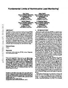
of buildings, research is underway on Building Energy Management System (BEMS) to reduce unnecessary energy consumption [5]. Depending on the external environment, air conditioners can be appropriately controlled to reduce the electric energy use. Unnecessary energy use can also be reduced through monitoring. In homes, the smart grid will be able to efficiently monitor and manage energy as it becomes increasingly realistic [6]. One approach to increasing the efficiency of domestic electricity use is to inspire positive behavioral change in consumers [7]. This can be achieved by analyzing energy use. Nonintrusive Load Monitoring (NILM) is one alternative to do so. NILM is a process for analyzing changes in the voltage and current going into a house and deducing which appliances are being used in the house along with their individual energy consumption. The initial concept of disaggregating residential power load information was proposed by Hart [8]. He demonstrated how different electrical appliances generate distinct power signatures, including their active power,

2

Computational Intelligence and Neuroscience

Power (KW)

4

Stove burner

3 Oven element

2

Refrigerator Oven element

1 Refrigerator

0

0

10

20 Time (min)

30

40

Figure 1: Basic concept of NILM [8].

current, and voltage (Figure 1). He showed how on-off events were sufficient to characterize the use of some appliances. Many researchers have studied this concept and improved the NILM model. In order to disaggregate a power consumption based on NILM, we have to understand features of appliances. Hart defined three types of appliance model according to the features. Three types are On/Off, Finite State Machine (FSM), and Continuously Variable [8, 9]. The first type On/Off has binary states of power such as a light and a toaster. Figure 2(a) shows the power pattern of light. When it is turned on, the power level is increased from 10 to 12 watts. The appliances of type 1 can be easily classified because of a clear feature. However, if two appliances which have similar power consumption are operating, they could not be distinguished. In this case, a classification model does not know which appliance is generating the current power. Therefore, we need an additional factor to distinguish them. The second type FSM has multiple states of power such as a lamp and a fan. The power pattern of lamp is shown in Figure 2(b). Three operation states are in lamp according to brightness. This kind of appliances can be modeled by FSM. So it could be simple to classify a single appliance of type 2. However, when the multiple power consumption is summed, the classification is become complicated, because it is hard to figure out that the current power is originated in the variable pattern. Therefore, we need to observe the pattern for a period of time in order to classify the appliances. The third type has a continuous changeable power pattern such as a washing machine and a light dimmer. In Figure 2(c), the power consumption is fluctuated while heating/washing or rinsing/drying a laundry. Strictly speaking, it is a multiple state appliance but it cannot be modeled due to infinite middle states. To classify type 3 appliances, we have to understand the feature and observe the long-range pattern. Lastly, we define an additional type Always On. The appliances of type 4 are always operating except a special case. For example, a refrigerator in Figure 2(d) is operating consistently. The type 4 appliances could have a periodic pattern or a single pattern. According to circumstances, we can reduce the number of appliances when we train the classification model. The main contributions in this work consist of two points. First one is a construction state-of-the-art NILM model. The

proposed model is robust against an increase of appliance due to the reduced time complexity. Although we use the low sample rate data, the multistate appliances and the similar power appliances can be classified efficiently. As learning a long-range power pattern result, we can solve the previous problems, which are mentioned in Section 3. We show that the proposed model outperforms via the experimental results with UK-DALE and REDD. Second one is a discovery of the novel signature. The proposed signature raises the performance of classification for the multistate appliance. By emphasizing the power variation when we train the model, the variation could be clearly trained. We show the efficiency via the validation experiments in Section 5.3. This paper is organized the structure as follows. We give problem statement from related works and proposed solutions in Section 2. Section 3 describes two NILM datasets to be used in our experiments. In Section 5, we conduct two main experiments. The first experiment is about validating the expected effects of the novel signature and learning architecture. The second experiment is about measuring the overall performance and comparing with the existing models and state of the art. Final section, we summarize our works and provide the conclusion.

2. Related Work 2.1. Signature Based Approach. There are two different kinds of signature. The first signature is the steady state. It makes use of steady-state features that are derived under the steadystate operation of the appliances. Hart proposed the concept of NILM and power change method at the same time in his paper [8]. In this method, real power (𝑃) and reactive power (𝑄) are used as the input signature. By computing changes of 𝑃 and 𝑄, the appliances are classified. Hart demonstrated how different electrical appliances generated distinct power consumption signatures. He showed how on/off events were sufficient to characterize the use of some appliances. The advantage of this method is that we can use a low sampling dataset and it is easy to identify the appliances having high power consumption. However, it is hard to classify the appliances having low power consumption and the multistate appliances which are types 2 to 4 in Figure 2. In addition to that, the appliances having similar power consumption cannot be classified. To improve NILM, other researches have attempted and proposed alternative signature identification techniques. Najmeddine et al. and Figueiredo et al. used the current 𝐼 and the voltage 𝑉 as the signature [11, 12]. They extracted the features such as Root Mean Square (RMS) of the current and peak. These features are well suited for classifying the appliances in the kitchen. However, the multistate appliances cannot be classified as ever. One of the signatures extracted from high sampling rate data is the harmonic of current. There are several researches acquiring the harmonics via Fourier series [13–16]. The appliances of types 1 and 4 are well classified by current harmonics. But it requires the harmonics set of all combinations of the appliances. As increasing the number of appliances, the harmonics for classification increase exponentially. This is not a practical approach and the memory problem could occur. There are

12 10 8 6 4 2 0

3 20 Power (watts)

Power (watts)


On Off

Off

0

100

200

300

400 500 600 Time (seconds)

700

800

15 10

State 2

5 0

900

State 3

State 1 Off

0

500

Type 1

1000

Power (watts)

Power (watts)

2000 1500

Heat, wash

1000

Rinse, dry Off

0

10

3000

3500

(b)

2500

0

2500

Type 2 (a)

500

1500 2000 Time (seconds)

20

30

40 50 60 Time (seconds)

70

80

90

Type 3

140 120 100 80 60 40 20 0

Freezing Defrosting

0

50

100

150

200

250

300

350

400

Time (seconds) Type 4

(c)

(d)

Figure 2: Four types of appliances. (a) Type 1 (On/Off): light; (b) type 2 (FSM): lamp; (c) type 3 (Continuously Variable): washing machine; (d) type 4 (Always On): refrigerator.

fancy approaches for NILM research. Lam et al. proposed the appliance categorization method based on the shape of 𝑉 − 𝐼 trajectory [17]. They categorized the appliances to eight groups with high accuracy. Gupta et al. tried to identify the appliances based on the noise generated from the operation of appliance [18]. However, the noise is easy to be affected by the environment. So it cannot be high efficient signature. In addition, we need to equip the device for measuring the noise. Therefore, it cannot be practical method. The second signature is the transient state. This signature is less overlapping in comparison with steady-state signatures. However, high sampling rate requirement in order to capture the transients is the major disadvantage. Chang et al. showed that the power consumption while an appliance is turning on can be calculated as a signature [19]. Five years later, they identified the transient physical behavior of power by using wavelet transform [20]. Another way for classification, Leeb et al. proposed the method analyzing the spectral envelope via Short Time Fourier Transform (STFT) [21]. In this way, the method of using transient power as a signature is suitable for classification of types 1 to 3. But it cannot catch type 4. Norford and Leeb showed that the shape of transient data can be a feature [22]. Cole and Albicki used power spikes generated from transition states [23]. This signature is efficient for classification but it is applied to several specific appliances. Like this, the method of using the current transient when the appliances are turning on is suitable for classification of types 1 and 2. But it cannot catch types 3 and 4. Patel et al. sampled the voltage noise extracted from the transient event [24]. They defined three

types of noise: on/off transient noise, steady-state line voltage noise, and steady-state continuous noise. However, to use this method, we need to have knowledge about the power flow such as the reactive power, the active power, and phase of voltage relative to current. The method using the voltage noise is suitable for classification of the multistate appliances. 2.2. Learning Model Based Approach. Some useful temporal graphical models, the variants HMM, are used for NILM. Zoha et al. proposed a solution using FHMM to recognize appliance specific load patterns from the aggregated power measurements [25]. They defined five features that are combinations of the power measurement such as the real power, reactive power, and voltage waveforms. They achieved the 𝑓-measure of 0.614 for five appliances when they use multistate FHMM. Kolter and Johnson also used FHMM for NILM [26]. They had collected their own dataset called REDD which will be explained in the Section 4. The average accuracy was 47.7%. To improve the researches using FHMM, a number of researchers have extended FHMM. Kim et al. developed probabilistic models of appliance behavior using variants of FHMM [27]. The variants are Factorial Hidden Semi-Markov Model (FHSMM), Conditional FHHH (CFHMM), and Conditional FHSMM (CFHSMM). Figure 3 shows the relationships between the variant FHMMs and their performance comparison. Kolter and Jaakkola used a combination of additive FHMM and difference FHMM [28]. For inferencing, they proposed an Additive Fractional Approximate MAP (AFAMAP) algorithm. They achieved the recall of 0.603 for 7

4

Computational Intelligence and Neuroscience 1.0

F-measure

0.9

FHMM

Distribution shape

0.8

0.7

FHSMM 0.6

Additional features 0.5 CFHMM

CFHSMM

2

3

Model CFHSMM CFHMM (a)

4 5 6 The number of appliances

7

8

FHSMM FHMM (b)

Figure 3: Variants of FHMM and performance results [10]. (a) Relationships between the variant FHMMs; (b) performance comparison.

appliances. Parson el al. proposed the variant of the difference HMM and the extended Viterbi algorithm [29]. Zeifman proposed a Viterbi algorithm with Sparse Transitions (VAST) [30]. And he used Markov chain (MC) for NILM.

3. Problem Statement and Proposed Solution 3.1. Problem Statement. The data for NILM is collected in a timed sequence. Therefore, the models dealing with a sequential data are used as an appliance classification model. The models which are usually used are Factorial Hidden Markov Model (FHMM) based on the Markov process and its variants [32]. However, these models have three problems to classify the appliances. The problems are as follows: (i) The first problem is about the time complexity. In case of FHMM, the time complexity is 𝑂(𝑀𝑛𝑀+1 𝑇) where 𝑀 is the number of appliances and 𝑛 is the possible states of hidden unit and 𝑇 is the length of observation sequence. As the number of appliances is increased, the time complexity is increased exponentially as well. This leads to reduction of the classification performance of the model. (ii) The second problem is about the difficulty of classifying the multistate appliance. The multistate appliance is the appliance which has the multiple state of power consumption. To distinguish them, a longrange pattern should be trained. However, the existing models are based on the first-order Markov process. Therefore, the pattern could not be trained efficiently. In addition, a low sample rate data (e.g., a collected data by 1∼6 Hz sample rate) is not proper for classifying the multistate appliances. If we use a high

sample rate data for NILM, this problem might be solved due to catching a momentary change of power consumption. But there is a limitation for the real life because a high cost device is needed for collecting the high sample rate data. (iii) The third problem is a difficulty of classifying the appliances having similar power consumption. If we use only power consumption as an observation of FHMM, the model could not distinguish the similar power appliances. We surveyed the basic models and the related works of NILM so far. However, there are some problems from the original basics of NILM. In this section, we summarized them into three. Problem 1. The researchers have used FHMM and the FHMM variants for NILM [25–27, 29]. As we know, the time complexity of FHMM is 𝑂(𝑀𝑛𝑀+1 𝑇) where 𝑀 is the number of appliances and 𝑛 is the possible states of hidden unit and 𝑇 is the length of observation sequence. Therefore, as increasing the number of appliances, the time complexity also increases exponentially. As a result, the performance of classification model is dropped. We can easily notice that in Figure 3(b). Problem 2. The second problem is that FHMM and the FHMM variants are hard to classify type 2 to 4 appliances. A long-term pattern is needed to learn but most models are based on the first-order Markov chain [35]. So these models predict the current state through the previous state. As a result, FHMM and the FHMM variants have a limitation for classifying the multistate appliances. In addition, there is another problem based on the signature perspective. In the

Computational Intelligence and Neuroscience signature based approach, we can separate the low sampling rate signature and the high sampling rate signature. The advantage of first signature is that we can easily collect the data from a simple sensor. However, the low sampling rate signature was unsuitable for classifying types 2 to 4 in the most researches [8, 11, 12]. To solve this problem, we need more precise data and high sampling rate signature. By this signature, the researchers classified all types of appliances. However, a specific device should be equipped in order to get the signature. It means that the high cost is required for application of the real life. This is not a good way for popularizing NILM. Problem 3. The last problem is the difficulty of classifying the appliances which have similar power consumption. In the previous models, the observation was only a series of power consumption. HSMM deals with a duration of operation but how can we know the durations for each appliance? The durations are not stable and it is a very tiresome business to extract the durations for each appliance. For example, in Figure 4, we extracted the patterns of air-conditioner from one house. We can notice that the duration is different. It depends on a user’s behavior. Through summarizing the problems, we concluded that the problems from FHMM and the FHMM variants are the fundamental issues from the architecture of FHMM. Therefore, we propose a deep learning based NILM model. Also, we propose the novel low sampling signature in order to apply to the real life. We have three challenges for successful application of deep learning. Challenge 1. Our model must be robust even though the number of appliances is increased. The significant problem of NILM models based on FHMM is that the performance is decreased as increasing the number of appliances. This will be the biggest obstacle for applying NILM to the real life. Therefore, the proposed model should be robust even though the number of appliances is increased. Challenge 2. The multistate appliance should be classified. The problem when we use a low sample rate data is that it is hard to classify the multistate appliances. This is caused by the fact that various patterns of appliance cannot be reflected efficiently to the main signal (total power consumption) due to a wide sampling gap. Although it is type 1 appliance, the main signal could be a multistate signal because of overlapping signal for each appliance. So we must classify the multistate appliances. Challenge 3. Although there are the appliances having the similar power consumption, they should be classified. If power consumption is the same between two appliances, they would be the same appliances. Except this case, the appliances having the similar power consumption can slightly be different. For the accurate performance, we need to distinguish the similar appliances.

5 3.2. The Proposed Solution 3.2.1. Proposed Novel Signature. Sequence data selected from real life might be power consumption sampled at 1 to 6 Hz. Because of the cost of a sensor, there is a limitation to collecting high sample rate data. To popularize NILM, we have to use low sample rate data from such a sensor. In Section 3, we acknowledge that it is hard to classify multistate appliances (type 2, type 3, and type 4) when using low sample rate data. To solve the problem, we propose a novel signature, which is a key input feature. The main idea of the signature is to separate the original signal, which is low sample rate data (power consumption), using a reflection rate and to subtract one variant power signal from the other variant power signal. We denote the difference as Δ 𝑝 which represents variation of the original signal. The purpose of Δ 𝑝 is to emphasize the variation of multistate appliances by applying the same importance with the original signal to a training model. The result is that performance of the model for an appliance with many variations may be better than when using only the original signal. To calculate Δ 𝑝 , we need to generate the variant power signal. The purpose of using the variant power signal is to reduce noise. An unintended noise can occur and it can have a negative influence on learning the signal pattern. We can regulate noise with the reflection rate. The reflection rate ranges from 0 to 0.99. Power signals that increase or decrease gradually are reflected to the variant power signal, while noise, which occurs in a moment, is not reflected well. This lower reflection rate reduces the negative effect of momentary noise. However, if the reflection rate is too low, the original power pattern may not be reflected. Thus, it is vital to set the reflection rate properly. Through the experiment explained in Section 5.3.1, we empirically found that 0.1 or 0.01 is the proper reflection rate. Algorithm 1 shows how to generate the variant power signal. There are two inputs for the algorithm: 𝑃 is the series of the original signal with the time length 𝑇 and 𝛼 is the reflection rate, which is a ratio for reflecting variation between the original signal and the variant power signal. The output 𝑉𝑃 is the variant power signal generated by the algorithm. In line (1), the variant power signal is initialized to zero. The generation process is given in lines (2) to (5). After the variation at time 𝑖 is calculated in line (3), it is reflected to the variant signal at reflection rate 𝛼 in line (4). Figure 5 is an example of the variant power signal. Figure 5(a) is the series of the original signal with the time length 5000. Figure 5(b) is the variant power signal when the reflection rate is 0.1. Note that the pattern is smoother than the original. This indicates that momentary noise has been reduced while long-range variations remain. Figure 5(c) is the variant power signal when the reflection rate is 0.01. In this case, the original signal changes are more slowly reflected to the variant power signal. With two different variant power signals, we can calculate the variations in the original signal. The algorithm for the novel signature is in Algorithm 2. Two variant power signals are the input and the novel signature representing the series of variation is the output. Δ 𝑝 is calculated by subtracting the inputs. In the scale of the

6


Power consumption (watt)

3500 3000 2500 2000 1500 1000 500

1 86 171 256 341 426 511 596 681 766 851 936 1021 1106 1191 1276 1361 1446 1531 1616 1701 1786 1871 1956 2041 2126 2211 2296 2381 2466 2551 2636 2721 2806 2891 2976 3061 3146 3231 3316 3401 3486 3571 3656 3741 3826 3911 3996 4081 4166 4251 4336 4421 4506 4591 4676 4761 4846 4931 5016

0

Time (sec) (a)


3500 3000 2500 2000 1500 1000 500

1 39 77 115 153 191 229 267 305 343 381 419 457 495 533 571 609 647 685 723 761 799 837 875 913 951 989 1027 1065 1103 1141 1179 1217 1255 1293 1331 1369 1407 1445 1483 1521 1559 1597 1635 1673 1711 1749 1787 1825 1863 1901 1939 1977 2015 2053 2091 2129 2167 2205 2243 2281 2319 2357 2395 2433 2471 2509 2547 2585

0

Time (sec) (b)


3000 2500 2000 1500 1000 500

1 132 263 394 525 656 787 918 1049 1180 1311 1442 1573 1704 1835 1966 2097 2228 2359 2490 2621 2752 2883 3014 3145 3276 3407 3538 3669 3800 3931 4062 4193 4324 4455 4586 4717 4848 4979 5110 5241 5372 5503 5634 5765 5896 6027 6158 6289 6420 6551 6682 6813 6944 7075 7206 7337 7468 7599 7730 7861 7992 8123 8254 8385 8516 8647 8778 8909 9040 9171 9302 9433 9564

0

Time (Sec) (c)

Figure 4: Different durations of air-conditioner: (a) duration: 5016 sec; (b) duration: 2585 sec; (c) duration: 9564 sec.

original signal, small variations are easily ignored. However, if we give Δ 𝑝 the same weight as the original signal, these small variations become more apparent than before. This effect of the novel signature will be validated in Section 5.3.2. Figure 6 represents a computation of Δ 𝑝 . By Algorithm 1, the variant power signals (Figure 6(b)) are generated from the original signal (Figure 6(a)). We can see that the patterns of the variant power signal differ according to the reflection rates. The variant power signals in Figure 6(b) can be the inputs for Algorithm 2. Finally, the series of variations, Δ 𝑝 , is generated by Algorithm 2. 3.2.2. Learning Architecture. In this section, we introduce how to apply deep learning to NILM. We choose RNN as the learning algorithm. RNN can learn the sequential data such as the power consumption of household. And we apply LSTM to hidden layer in order to prohibit the vanishing

gradient problem. We call this model LSTM-RNN. There are two reasons for applying deep learning to NILM. The first reason is that the time complexity was getting higher as the number of appliances was increased in the FHMM variants. The time complexity of FHMM is 𝑂(𝑀𝑛𝑀+1 𝑇) where 𝑀 is the number of appliances and 𝑛 is the possible states of hidden unit and 𝑇 is the length of observation sequence. As we can see, the number of appliances has a close relation with the time complexity. As a result, the performance was dropped as the number of appliances was increased. In deep learning, the major time complexity is originated from backpropagation. Stochastic Gradient Decent (SGD) is usually used for backpropagation [36]. As a result, the time complexity of SGD is 𝑂(𝑚𝑑). In our model, the output dimension is the number of appliances. So the time complexity is not increased exponentially in contrast with FHMM. If we use the deep learning based NILM model, the model could be

4500 4000 3500 3000 2500 2000 1500 1000 500 0

7

6000 Power (watts)

Power (watts)


0

1000


4000

5000 4000 3000 2000 1000 0

5000

0

P (original signal)

1000


4000

5000

8000

10000

VP with reflection rate = 0.1 (b) Variant power signal with 𝛼 = 0.1

(a) Original power signal (load)

Power (watts)

6000 5000 4000 3000 2000 1000 0

0

1000


4000

5000

VP with reflection rate = 0.01 (c) Variant power signal with 𝛼 = 0.01

3000 2500

Power (watts)

3000 2500 2000 1500 1000 500 0

0

2000


8000

2000 1500 1000

Delta

500

10000

0

0

P (original signal)

2000


VP with reflection rate = 0.1 VP with reflection rate = 0.01

(a) Original power signal (load)

Power (watts)

Power (watts)

Figure 5: Patterns of the variant power signals.

1200 1000 800 600 400 200 0 −200 −400 −600

0

(b) Difference of the variant signals

2000


8000

Delta(P) (c) Pattern of Δ 𝑝

Figure 6: Computing Δ 𝑝 from the variant signals.

10000

8


Washer

Washer

450 400 350 300 250 200 150 100 50 0 1 7 13 19 25 31 37 43 49 55 61 67 73 79 85 91 97 103 109 115 121 127 133 139 145 151 157 163 169 175 181 187 193 199 205 211 217 223 229 235 241 247 253 259 265 271 277 283 289 295 301 307 313 319 325 331 337 343 349 355 361 367 373 379 385 391 397 403 409 415 421 427 433 439 445 451 457 463 469 475 481 487 493 499


Washer

Time (sec)

ot−1

ot

ot+1

ℎt−1

ℎt

ℎt+1

xt−1

xt

xt+1

Act as memory

Figure 7: Long-range pattern learning.

Require: 𝑃 = 𝑝1 , 𝑝2 , . . . , 𝑝𝑇 , Reflection rate 𝛼 Ensure: VP = vp1 , vp2 , . . . , vp𝑇 (1) VP ← 0 (2) for 𝑖 = 2 to T do (3) 𝑑 ← 𝑝𝑖 − vp𝑖−1 (4) vp𝑖 ← vp𝑖−1 + 𝛼 ⋅ 𝑑 (5) end for (6) return VP

Require: VP1 = vp11 , vp12 , . . . , vp1𝑇 , VP2 = vp21 , vp22 , . . . , vp2𝑇 Ensure: Δ 𝑝 = 𝛿1 , 𝛿2 , . . . , 𝛿𝑇 (1) for 𝑖 = 2 to T do (2) 𝛿𝑖 ← vp1𝑖 − vp2𝑖 (3) end for (4) return Δ 𝑝 Algorithm 2: Computing algorithm for the novel signature.

Algorithm 1: Generation algorithm for the variant power signal.

robust relatively. Additionally, deep learning uses the parallel computing via GPU. It means that even though the time complexity is high, GPU can reduce it. This is one of the major reasons why many researchers have been fascinated by deep learning. For the record, the latest GPU, Titan X with Pascal Architecture, has 3584 cores, 12 GB memory, and 11 GFLOP. The second reason is that the long-term pattern cannot be learned in the FHMM variants (see Figure 7), because they are

based on the first-order Markov chain. On the other hand, the hidden layer of LSTM-RNN is a kind of memory. A washer is the representative of the multistate appliance. Although the pattern is long and changeable, it could be learned when we set a length of LSTM-RNN similarly. This feature could classify the multistate appliances and the appliances having the similar power consumption. We realized that the NILM model based on deep learning has a high possibility of achieving three challenges. One


9

important thing when using LSTM-RNN model is how to choose the suitable factors of this model. Here we discover four factors, which are considered much effective in our model. Preprocessing Method. Generally, 𝑍-Score method and Min–Max Scaling are considered as a normalization method for deep learning. In deep learning, a model has better performance when a distribution of input data is close to Gaussian distribution. Min–Max Scaling is the most simple way to normalize the input data. It converts the scale in range from 0 to 1 by using the minimum and maximum value. This method holds the original distribution but it cannot be the Gaussian distribution. 𝑍-Score method normalizes the input data by using the mean and standard deviation. This method cannot hold the original distribution when the input distribution is not the Gaussian. Nevertheless, it is important that the mean of input data is close to zero, because if the input is all positive or negative, the weight could be updated in one way. In case of NILM, one of inputs, power consumption, is all positive value. Therefore, we use 𝑍-Score as the preprocessing method. We are going to take an experiment about the preprocessing method in Section 5.4.1. Weight Initialization Method. Asymmetry is the most important thing for the weight initialization. We can simply think that if the weights are initialized to zero, the update could be clear. But soon we realize that this method is wrong. There are only bias values in forward propagation. The simplest way to initialize the weights with asymmetry is selecting values from normal distribution or uniform distribution. However, this method has the problem that a variance of output increases with an input dimension. To solve this problem, the variance of output needs to be divided by the square root of input dimension. By this way, Glorot initialization and He initialization are commonly used for the weight initialization. The simple equations of them are as follows: 𝑊glorot = 𝑊he =

random (fanin , fanout ) √fanin random (fanin , fanout ) √fanin /2

, (1) ,

where fanin and fanout are the number of input and output dimensions and 𝑟𝑎𝑛𝑑𝑜𝑚 is a function of random selection in range from fanin to fanout from normal distribution or uniform distribution. Both equations are similar but He initialization selects the weight values in wide range relatively. In deep neural network like RNN, the weight can easily be shrunk to nothing when the values are close to zero. This leads to vanishing gradient problem. Therefore, we use He initialization due to the wide range value. A related experiment will be conducted in Section 5.4.2. Activation Function. In general, the softmax is used as an activation function for multiclass classification [37]. It can select a one class among all classes. However, in NILM, many appliances could have been operated in the same time. It

means that we need to classify the multiple classes. Therefore, we set the boundary with assuming that the appliance is turned on when the output unit value is bigger than the boundary. To do this, we change the softmax to the hyperbolic tangent (tanh) as the activation function. By this way, we can classify the multiple appliances at the same time. The sigmoid can also be the activation function. However, while the output of sigmoid is not zero-centered, the tanh has the zero-centered output. As a result, we could set the static boundary when we use tanh as the activation function. Optimizer. There are three optimizers for SGD. One of them is Adagrad. It decreases a learning rate when a signal is frequent or the weight has a high gradient. In the opposite case, it increases the learning rate. However, this method has a low performance due to decreasing the learning rate fast. RMSProb solves this problem by an exponential moving average. Adam is a combination of RMSProb and Momentum. It is known as the most efficient method for SGD. Therefore we use Adam as an optimizer. The inputs are the original signal (power consumption) and Δ 𝑝 . The output unit represents the on/off state of each appliance. By using the novel signature Δ 𝑝 , we can expect the better performance for classification of multistate appliances. We apply dropout between the input layer and the hidden layer in order to prevent overfitting. This is the simplest way to regularize the weights and is suitable for deep neural networks like an RNN. We set the number of hidden units to be double the number of output units. A small number of hidden units require more training epochs, whereas a larger number of hidden units require more computation time per epoch. We found that double the number of output units is a proper number for the NILM model through heuristic experiments. Based on these methods, we construct the architecture of an LSTM-RNN for NILM (Figure 8).

4. Dataset Description There are several public datasets for NILM. Table 1 shows descriptions for them. Among them, we concentrated on two datasets such as REDD and UK-DALE because of proper for NILM. Beside the public dataset, we had collected 6 appliances and aggregate data during 5 months. We are going to use our private dataset as well. The UK-DALE was released in 2014 at first and it has been updated every year [38]. There are power data for 5 households and each house has the different first measurement date. House 1 includes 3.5-year power data for 52 appliances. The 16 kHz data will not be used in this paper. And houses 1, 2, and 5 include 1-second data but there are no labeled data. Therefore we will not use 1-second data as well. We give an explanation for the 6-second data. Table 2 shows the detailed description of UK-DALE. House 1 has the large number of appliances. As the number of appliances is increased, a NILM model is hard to distinguish the appliances. But the disadvantage can be overcome because of much data. On the other hand, houses 3 and 4 have the small number of meters. The difference between of them is that a meter of house 4 is shared. For example, “tv dvd digibox lamp” means that

10

Computational Intelligence and Neuroscience Table 1: Public datasets for NILM [31].

Dataset REDD (2011) BLUED (2012) Smart (2012) Tracebase(2012) Sample (2013) HES (2013) AMPds (2013) iAWE (2013) UK-DALE (2016)

Number of houses 6 1 3 N/A 10 251 1 1 5

Duration per house 3–19 days 8 days 3 months N/A 7 days 1 or 12 months 1 year 73 days 1–3.5 years

；ＪＪ1

Appliance sample frequency 3 sec N/A 1 sec 1–10 sec 1 min 2 or 10 min 1 min 1 or 6 sec 6 sec or 16 kHz

；ＪＪ2

；ＪＪo−1 Activation

tanh

Weight init.

He’s initialization

Optimizer

Adam

t= t+1

Aggregate sample frequency 1 sec, 15 kHz 12 kHz 1 sec N/A 1 min 2 or 10 min 1 min 1 sec 1 or 6 sec, 16 kHz

；ＪＪo

Applied LSTM ℎ1

ℎ2

ℎ3

ℎm−2

Activation Weight init.

tanh He’s initialization

Regularization

Dropout

ℎm−1

ℎm

m= 2×o

Δp

P

Preprocessing Z-Score

Figure 8: LSTM-RNN for NILM.

the 4 appliances are using the same meter. When the NILM model is trained by a dataset, the shared meter may cause a confusion or make a distinguishable pattern. In Section 5, we can confirm the effect of the shared meter. The REDD is the first public dataset for NILM [26]. The major purpose of REDD is the standard dataset for benchmarking the NILM algorithms. In REDD, there are AC waveform data with sampling rate of 15 kHz. Therefore, REDD can be used for each approach using the high or low sampling data. It is sampled from six different houses in Massachusetts of the United States. There are three categorized data, low freq, high freq, and high freq raw. We are going to use low freq data in this paper. Each house’s dataset is composed of the main phases sampled 1 Hz and the individual data of each appliance sampled 3 or 4 Hz. Table 3 shows the detailed description of REDD. Each house has the appliance in range from eleven to twenty-six. We renamed the same appliances like kitchen outlets1 and kitchen outlets2.

The problem of UK-DALE and REDD is the asynchronization between a total load and each appliance data due to the different sample rate. So we have to synthesize each appliance data for generating an output dataset. When we collect the data from the real household, noise can be included in the total load. However, the synthesized data is not affected on the noise. To solve the problem, we collect the data of six appliances for five months. The description of the private data is in Table 4.

5. Experiment 5.1. Experiment Description. The purpose of the experiment is to satisfy three challenges defined. The challenges are as follows. Challenge 1. Our model must be robust even though the number of appliances is increasing.


11

Table 2: The detailed description of UK-DALE. House

Date of first measurement

Submeters

1

2012-11-19

53

2

2013-02-17

20

3

2013-02-27

5

4

2013-03-09

6

5

2014-06-29

26

Appliances Boiler, solar thermal pump, laptop, washing machine, dishwasher, tv, kitchen lights, htpc, kettle, toaster, fridge, microwave, lcd office, hifi office, breadmaker, amp livingroom, adsl router, livingroom s lamp, soldering iron, gigE & USBhub, hoover, kitchen dt lamp, bedroom ds lamp, lighting circuit, iPad charger, subwoofer livingroom, livingroom lamp tv, and so on Laptop, monitor, speakers, server, router, server hdd, kettle, rice cooker, running machine, laptop2, washing machine, dish washer, fridge, microwave, toaster, playstation, modem, cooker Kettle, electric heater, laptop, projector Tv dvd digibox lamp, kettle radio, gas boiler, freezer, washing machine microwave breadmaker Stereo speakers, desktop, hairdryer, primary tv, 24 inch lcd, treadmill, network attached storage, server, 24 inch lcd bedroom, PS4, steam iron, nespresso pixie, atom pc, toaster, home theatre amp, sky hd box, kettle, fridge freezer, oven, electric hob, dishwasher, microwave, washer dryer, vacuum cleaner

Table 3: The detailed description of REDD. House

Submeters

1

20

2

11

3

22

4

20

5

26

6

17

Appliances Oven1, oven2, refrigerator, washer drye1, dishwasher, kitchen outlets1, kitchen outlets2, lighting, lighting1 washer dryer2, microwave, bathroom gfi, electric heat, stove, kitchen outlets3, washer dryer3kitchen outlets4, lighting2 Kitchen outlets1, lighting, dishwasherstove, microwave, washer dryer, kitchen outlets2, refrigerator, disposal Outlets unknown1, kitchen outlets1outlets unknown2, lighting 1, microwave, electronics, refrigerator, disposal, dishwasher, furance, lighting2, lighting3, outlets unknown3, washer dryer1, washer dryer2, lighting4, smoke alarms, lighting5, bathroom gfi, kitchen outlets2 Lighting1, furance, kitchen outlets1, stove, outlets unknown, washer dryer, air conditioning1, air conditioning2, miscellaeneous, smoke alarms, lighting2, kitchen outlets2, dishwaser, bathroom gfi1, bathroom gfi2, lighting3, lighting4, air conditioning3 Microwave, lighting1, outlets unknown1, furance, outlets unknown2, washer dryer1, washer dryer2, subpanel1, subpanel2, electric heat1, electric heat2, lighting2, outlets unknown3, bathroom gfi, lighting3, refrigerator, lighting4, dishwaser, disposal, electronics, lighting5, kitchen outlets1, kitchen outlets2, outdoor outlets Kitchen outlets1, washer dryer, stove, electronics,bathroom gfi, refrigerator, dishwasher, outlets unknown1, outlets unknown2, electric heat, kitchen outlets2, lighting, air conditioning1, air conditioning 2, air conditioning3

Challenge 2. The multistate appliance should be classified as well. Challenge 3. The similar power consumption in appliances should be classified. In this section, we take two validation experiments for the proposed signature and learning method and one performance measurement experiment. The first validation experiment consists of two subtests. The first one is a heuristic approach test for the optimized reflection rate. In this test, we compute three different Δ 𝑝 by three different reflection rates. By using Δ 𝑝 s, we train the models with the same condition. The second subtest is related to challenge 2. In

Section 3.2.1, we expected that the novel signature could classify the multistate appliances having many variations. To validate this, we train two models having {𝑃} and {𝑃, Δ 𝑝 } as inputs for each. And then we analyze the results. The second validation experiment is related to challenges 1 and 3. This experiment consists of four subtests. In the first subtest, we are going to find an optimized preprocessing method. 𝑍-Score normalization and Min–Max Scaling are popular methods for preprocessing. There is no rule which one is proper for a specific situation. So we experiment them for choosing the optimized method. The second subtest is about choice of the weight initialization methods. Among the initialization methods, the Glorot initialization and the

12

Computational Intelligence and Neuroscience evaluating the NILM model. The formulas to compute the value of them are given by

Table 4: Private dataset. House

1

Date of first measurement

Submeters

Appliances

6

Air-con., dehumidifier, TV, washer, toaster, oven

2016-03-11

Positive (predicted)

Negative (predicted)

Recall =

TP , TP + FN

Precision =

TP , TP + FP

TP + TN , Accuracy = (TP + FP) + (FN + TN) 𝐹1-score = 2 ∗

Positive (actual)

TP

Negative (actual)

FP

FN

TN

Figure 9: Confusion matrix.

He initialization are well known for providing good performance. But it is not revealed that which one is better or not. Therefore, we train two models with only changing the initialization method and compare the result. In the third subtest, we compare the performance as the number of appliances is increased. We could confirm that our model is robust even though the number of appliances is increased. In the last subtest, we synthesize the sampled data of appliances having the similar power consumption. Then, we confirm that the appliances are well classified or not. The last experiment is about measuring the overall performance. We are going to use the UK-DALE and REDD as the training/test data and measure the performance for each house in the dataset. Also, we take the same experiment by FHMM and compare the result. All models used in the experiment are implemented with Python programming and Theano library. 5.2. Performance Metrics. Up to now we have generally assumed that the best way of measuring the performance of a classifier is by its predictive accuracy, that is, the proportion of unseen instances it correctly classifies. However, predictive accuracy on its own is not a reliable indicator of a classifier’s effectiveness. As well as the overall predictive accuracy on unseen instances it is often helpful to see a breakdown of the classifier’s performance; it is a confusion matrix which is proposed by Kohavi and Provost, in 1998 [39]. Confusion matrix is described in Figure 9, including four categories. True positive (TP) is examples correctly labeled as positive. False positive (FP) refers to negative examples incorrectly labeled as positive. True negative (TN) corresponds to negatives correctly labeled as negative. Finally, false negative (FN) refers to positive examples incorrectly labeled as negative. We assume that the positive state means that an appliance is turned on. When the appliance is turned off, we regard it as a negative state. Based on the confusion matrix, we can calculate 𝑅𝑒𝑐𝑎𝑙𝑙, 𝑃𝑟𝑒𝑐𝑖𝑠𝑖𝑜𝑛, 𝐴𝑐𝑐𝑢𝑟𝑎𝑐𝑦, and 𝐹1-𝑠𝑐𝑜𝑟𝑒 for

(2)

Precision ∗ Recall . (Precision + Recall)

Recall is a ratio of the number of correct classifications to the total number of actual positive instances. A meaning of that Recall is high and the appliances are well classified by the NILM model when the actual instances are positive. Precision is a ratio of the number of correct classifications to the total number of predicted positive instances. A meaning of that Precision is high and a probability of well classification is high when the NILM model predicts the positive instances. Accuracy is a ratio of correct classification to the total test data. 𝐹1-𝑠𝑐𝑜𝑟𝑒 is the harmonic average of Recall and Precision. 5.3. Proposed Signature Validation Experiment 5.3.1. Optimum Reflection Rate. To find an optimum reflection rate, we set three different reflection rates, 0.1, 0.01, and 0.001, and compute three variant signals. For experiment, we randomly select the 15 appliances from UK-DALE. By using the variant signals, we calculate three Δ 𝑝 . Δ 𝑝 1 is a result of subtraction of the first signal and the second signal. Δ 𝑝 2 is a result of subtraction of the first signal and the third signal. Δ 𝑝 3 is a result of subtraction of the second signal and the third signal. Figure 10 shows the pattern of each Δ 𝑝 . Intuitionally, Δ 𝑝 2 and Δ 𝑝 3 are biased. The values of each Δ 𝑝 are detailed in Table 5. We can notice that the mean of Δ 𝑝 1 is close to zero unlike the others. A variance and standard deviation of Δ 𝑝 1 are almost in middle of the others. And the scale of range of Δ 𝑝 1 and Δ 𝑝 2 is similar. We could know which one is proper to NILM by a comparison experiment. Table 6 shows performance results. All performances are similar except that Δ 𝑝 1 is better than the others. Therefore, we will use (0.1, 0.01) as a reflection rate. 5.3.2. Effect of the Novel Signature. In this section, we train the two models having {𝑃} and {𝑃, Δ 𝑝 } as an inputs for each. We extracted 72-day data as a training dataset and 30-day data as a test dataset. Each model was trained 2000 epochs. As we explained in Section 4, the private dataset has six appliances. Actually, these appliances are not operating in the same time. However, in our work, we assumed that multiple appliances could have been operated in the same time. Therefore, 26 = 64 which is the number of combinations of all appliances. We represented the on/off state by the binary representation. And we change the output unit values to one binary string. After that, the string is converted to a decimal number that stands for the combination. A sequence of appliances is {Air-conditioner, Washer, Dehumidifier, Oven, TV, Toaster}.

3500 3000 2500 2000 1500 1000 500 0 −500 −1000

13

Power (watts)

Power (watts)


0

5000

10000 Time (seconds)

15000

20000

3500 3000 2500 2000 1500 1000 500 0 −500 −1000

Delta 2

0

5000


15000

20000

Delta 1 (b)

Power (watts)

(a)

3500 3000 2500 2000 1500 1000 500 0 −500 −1000

0

5000


15000

20000

Delta 3 (c)

Figure 10: Comparison of Δ 𝑝 . (a) Pattern of Δ 𝑝 1; (b) pattern of Δ 𝑝 2; (c) pattern of Δ 𝑝 3. Table 5: Statistic of Δ 𝑝 . Δ𝑝 Δ 𝑝1 Δ 𝑝2 Δ 𝑝3

Range (−841∼2510) (−411∼3149) (−366∼1040)

Mean 1.047 −13.361 −14.358

For example, if the washer and toaster are operating, the binary string would be {010001} and the combination number would be 17. Figure 11 shows the classification ratio comparison between the models. The 𝑥-axis is a combination and the 𝑦axis is a classification ratio. We can easily notice that if we use the proposed signature additionally, the more combinations could be classified. 30 combinations were classified when we use the proposed signature whereas 11 combinations were classified when we use only power consumption (not all combinations are included in the dataset). Figure 12 shows the performance of each appliance. The second model using {𝑃, Δ 𝑝 } has the better performance in all appliances except the dehumidifier. Particularly, there are large gaps in the washer, oven, and toaster. The operation time for the oven and toaster is only 1.5 hours and 2.8 hours during 30 days. Even though the sample number is small, the second model has the better performance relatively. However, the dehumidifier performance of first model is higher than that of the second one. We see this performance in Figure 13. The pattern of dehumidifier is simple. A fluctuating Δ 𝑝 could be efficient for learning the pattern but the other case is not. Because the importance of Δ 𝑝 is the same with

Variance 83116.404 140077.047 34845.009

Standard deviation 288.299 374.268 186.668

the power consumption, this kind of simple pattern could be learned slowly. To confirm this, we trained 2000 epochs more for the second model. In Table 7, the performance of dehumidifier is improved from 0.65 to 0.82 whereas the other performances are similar with before. Because the washer has fluctuating Δ 𝑝 , the performance of the second model is about double. As a result, the proposed signature could be very efficient factor for classifying the multistate appliances. 5.4. Deep Learning Model Validation 5.4.1. Optimum Preprocessing Method. 𝑍-Score normalization and Min–Max Scaling are popular methods for preprocessing. However, it has not revealed which one is better. To find an optimum method for NILM, we train the two different models. The datasets for all models are the same. We extracted 23-day data from house 5 of UK-DALE. 17-day data is used as a training dataset and 6-day data is used as a test dataset. Each model trains 1000 epochs. Figure 14 shows the performance results of the models. We can notice that 𝑍-Score method has the better performance than Min–Max Scaling. In NILM, one of the inputs is the power consumption. As we know, all power consumption

14

Computational Intelligence and Neuroscience Table 6: Performance measurement with different reflection rates.

Δ 𝑝 (reflection rate) Δ 𝑝 1 (0.1, 0.01) Δ 𝑝 2 (0.1, 0.001) Δ 𝑝 3 (0.01, 0.001)

Precision 0.753 0.714 0.730

Recall 0.843 0.836 0.812

𝐹1-Score 0.795 0.771 0.769

Accuracy 0.901 0.886 0.888

100 90 80

Classification ratio (%)

70 60 50 40 30 20 10 0

1 2 3 4 5 6 7 8 9 10 11 12 13 14 15 16 17 18 19 20 21 22 23 24 25 26 27 28 29 30 31 32 33 34 35 36 37 38 39 40 41 42 43 44 45 46 47 48 49 50 51 52 53 54 55 56 57 58 59 60 61 62 63

Combinations P

Zero instances

(P, Δ)

Below 10 instances

Figure 11: Classification ratio comparison {𝑃}, {𝑃, Δ 𝑝 }.

Appliance Air-conditioner Washer Dehumidifier Oven TV Toaster

𝐹1-Score 0.89 0.67 0.82 0.55 0.70 0.49

is positive. If all input data are the positive value, all weights could be increased or decreased when the backpropagation is processed. As a result, the dataset for NILM should be standardized. As expected in Section 3.2.2, 𝑍-Score method is proper for preprocessing. 5.4.2. Optimum Weight Initialization Method. Among the weight initialization methods introduced, the researchers usually use Glorot initialization and He initialization. But they still have argued about the better method between two methods. The methods use a similar theoretical analysis. They found a good variance for the distribution from which the initial parameters are drawn. This variance is adapted to the

F1-score

Table 7: The performance of second model (4000 epochs).

1 0.9 0.8 0.7 0.6 0.5 0.4 0.3 0.2 0.1 0

0.88 0.87

0.81 0.65

0.7

0.65

0.62 0.56 0.49

0.29 0.13

0.07

Ari-condition

Washer

Dehumidifier

Oven

TV

Toaster

Appliance P (P, Δ)

Figure 12: Classification performance of the appliances.

activation function used and is derived without explicitly considering the type of the distribution. As such, their theoretical conclusions hold for any type of distribution of the determined variance. To compare the weight initialization methods, we applied the same distribution (uniform distribution) to the methods. We extracted 71-day data from the private dataset. 50-day data are used as a training dataset and 21-day data are used as a test dataset. We train two models


15

800


700

600

500

400

300

200

100

0 1

9

17

25

33

41

49

57

65

73

81

89

97 105 113 121 129 137 145 153 161 169 177 185 193 201 209 217 225 233 241 249 257

Time (sec) (a) 450

400


350

300

250

200

150

100

50

1 7 13 19 25 31 37 43 49 55 61 67 73 79 85 91 97 103 109 115 121 127 133 139 145 151 157 163 169 175 181 187 193 199 205 211 217 223 229 235 241 247 253 259 265 271 277 283 289 295 301 307 313 319 325 331 337 343 349 355 361 367 373 379 385 391 397 403 409 415 421 427 433 439 445 451 457 463 469 475 481 487 493 499

0

Time (sec) (b)

Figure 13: The patterns of dehumidifier and washer: (a) dehumidifier; (b) washer.

1 0.9 0.8 0.7 0.6 0.5 0.4 0.3 0.2 0.1 0

0.88 0.79

0.84

0.91 0.88

0.74

Precision

Recall Accuracy Performance metrics

0.84

0.79

F1-Score

Z-Score Min–Max

Figure 14: Comparison of the preprocessing methods.

during 1000 epochs for each and set a time step to be 500, a loss function to be MSE, and optimization to be Adam.

Table 8 shows the result of experiment. The precision of Glorot initialization is much higher than the precision of He initialization. In case of the recall, He’s method is higher than Glorot’s method. The model which used Glorot initialization has a high hit rate but a number of classified samples are low. The model which used He initialization has a low hit rate but a number of classified samples are high. The accuracy and 𝐹1-Score are similar. Before we select the method, we trained the models during 5000 epochs for each. Table 9 shows the results. After training more than 4000 epochs, the precision of He’s method is much improved than the previous result even though the recall is dropped. However, the model which used Glorot initialization is not much improved in all metrics. He initialization was proposed in case the input data is positive. The power consumption is all positive values but Δ 𝑝 is not. We could not convince He initialization. But guessing from the result, we can know that He initialization

16

Computational Intelligence and Neuroscience Table 8: Performance comparison of initialization methods (1000 epochs).

Metric Precision Recall Accuracy 𝐹1-Score

He initialization 0.529 0.775 0.934 0.629

Glorot initialization 0.962 0.456 0.959 0.619

Table 9: Performance comparison of initialization methods (5000 epochs). Metric Precision Recall Accuracy 𝐹1-Score

He initialization 0.954 0.535 0.964 0.685

Table 10: Control parameters for experiment. Control parameter Input Num. of training samples Num. of test samples Time step Num. of epochs Cost function Optimization Preprocessing Weight init. Regularization

Method 𝑃, Δ 𝑝 1,500,000 500,000 500 1000 Mean Squared Error Adam 𝑍-Score He initialization Dropout

is efficient for NILM. As a result, we will use He initialization as the weight initialization method. 5.4.3. Performance Measurement with Increasing the Number of Appliances. In this section, we are going to take an experiment for confirming the robustness of proposed model even though the number of appliances is increased. In the experiment, we hold all parameters except the number of appliances. The control parameters are in Table 10. The fifteen appliances for measuring the performance are selected from house 5 of UK-DALE (Table 20). Table 11 shows the appliances used for each experiment. To observe the performance precisely, we synthesize the data of appliances with adding one appliance to the previous ones. Figure 15 shows the result of experiment. The 𝑥-axis is the number of appliances. The 𝐹1-Score representing the overall performance of the model is decreased from 2 to 9. However, after 9 appliances, the 𝐹1-Score pattern walks up and down in range from 0.8 to 0.9. Due to the high performance, the 𝐹1Score is going down in the early phase. However, it is going up and down in the late phase. Therefore, we cannot conclude that the model is influenced by the number of appliances. We compare the two models; those numbers of appliances are 13 and 14 for each. The 𝐹1-Score of first model is 0.822 but it is increased to 0.866 when the 14 appliances are trained. The added appliance is home theatre amp. The total operation

Glorot initialization 0.954 0.466 0.960 0.626

1.2 1 0.8 0.6 0.4 0.2 0 2

3

4

Precision Recall

5

6

7 8 9 10 11 12 13 14 15 Number of appliances Accuracy F1-Score

Figure 15: The result of performance measurement model in increasing appliances.

time is about 68 hours and we can notice that the appliance has many variations in Figure 16. On the other hand, the 𝐹1Score is going down when the number of appliances is from 7 to 8. The added appliance is core2 server. We can notice that the power pattern is monotonous in Figure 17. Therefore, we can think that the major factor affecting on the performance is the data. As a result, we can conclude that the proposed model for NILM is robust against the number of appliances. 5.4.4. Performance Measurement of Appliances Having the Similar Power Consumption. In this section, we are going to take an experiment for confirming that the appliances having a similar power consumption are well classified by the NILM model. If the similar power appliances are operating in a different time, the model could be hard to classify them. However, the power consumption and the operation time are slightly different even though the appliances are the similar power appliance. The power gap would be emphasized by the proposed signature and the operation time could be memorized in the hidden neurons of the proposed model. To validate our assumption, we collected the 11 numbers of the similar power appliances from UK-DALE and synthesized their data in Table 11. And the control parameters are the same with the previous experiment (Table 10). Table 12 shows the result of performance measurement. We can see that they


17

Table 11: A List of the similar power appliances. Number (1) (2) (3) (4) (5) (6) (7) (8) (9) (10) (11)

Appliance adsl router Data logger pc hifi office Livingroom lamp tv Livingroom s lamp2 Modem Office lamp1 Office lamp2 Server-hdd Speaker Subwoofer livingroom

Power range (watt) 6∼7 12∼13 12∼14 11∼14 7∼9 9∼10 14 9∼10 10∼13 10∼11 15∼16

120


100

80

60

40

20

1 3111 6221 9331 12441 15551 18661 21771 24881 27991 31101 34211 37321 40431 43541 46651 49761 52871 55981 59091 62201 65311 68421 71531 74641 77751 80861 83971 87081 90191 93301 96411 99521 102631 105741 108851 111961 115071 118181 121291 124401 127511 130621 133731 136841 139951 143061 146171 149281 152391 155501 158611 161721 164831 167941

0

Time (sec)

Figure 16: Power pattern of home theatre amp.

Table 12: Result of performance measurement for classification of similar power appliance. Metric Precision Recall Accuracy 𝐹1-Score

Similar power appliance based model 0.955 0.948 0.957 0.951

are well classified even though they are the similar power appliances. To validate our assumption, we collected the 11 numbers of the similar power appliances and 3 numbers of the multistate appliances having a high power consumption from UKDALE and synthesized their data in Table 13. And the control parameters are the same with the previous experiment (Table 10). We train two models. The first one is the model using only similar power appliances. In the second model, the multistate appliances are included additionally. As we expected, we can observe that the performance is going down from the first model to the second model in Table 14. Although the performance is decreased, we can realize that.

5.5. Performance Comparison with the Existing Models. We could confirm that our proposed signature and model are efficient for NILM through the validation experiments. In this section, we would like to compare the performance with the existing models. We take an experiment for all houses in UKDALE and REDD. Firstly, we train all houses of UK-DALE and the result will be compared with FHMM. The parameters for UK-DALE experiments are in Table 15. Table 16 shows the overall performance of UK-DALE houses. The house having the lowest performance is the first house. We proved that our model is affected by the data. There are 53 appliances in the first house. The possibility of being the appliance data decreasing the performance is higher than the other houses. For example, the usage of battery charger and breadmaker is very rare. This kind of appliance is the major reason for dropping the performance. We compare the performance with FHMM by implementing it. The result is shown in Table 17. We can notice that our model is outperforming FHMM. The performance is almost double in most houses. Secondly, we train all houses of REDD and the result will be compared with the existing models. The results are good in all houses (see Table 18). We compare our model with

18

Computational Intelligence and Neuroscience Table 13: A List of the similar power appliances with adding three multistate appliances.

Number (1) (2) (3) (4) (5) (6) (7) (8) (9) (10) (11) (12) (13) (14)

Appliance adsl router Data logger pc hifi office Livingroom lamp tv Livingroom s lamp2 Modem Office lamp1 Office lamp2 Server-hdd Speaker Subwoofer livingroom Fridge Gas oven Hoover

Power range (watt) 6∼7 12∼13 12∼14 11∼14 7∼9 9∼10 14 9∼10 10∼13 10∼11 15∼16 85∼252 14∼52 500∼2021

Table 14: Result of performance measurement for classification of similar power appliances with adding three multistate appliances. Metric Precision Recall Accuracy 𝐹1-Score

Similar power appliance based model 0.955 0.948 0.957 0.951

Table 15: Parameters for UK-DALE experiment. Parameter Input Time step Num. of epochs Cost function Optimization Preprocessing Weight init. Regularization

Method 𝑃, Δ 𝑝 500 3000 Mean Squared Error Adam 𝑍-Score He initialization Dropout

three existing models such as FHMM, Additive FHMM, and HieFHMM [28, 32]. Among them, HieFHMM is the stateof-the-art model [34]. Due to few numbers of appliances, the existing models did not test house 2. Similar to UK-DALE result, our model has the highest performance in all houses. In case of house 4, our performance is double compared to that of state of the art. We can confirm this in Table 19.

6. Conclusions In this paper, we considered advanced deep learning is new approach to build state-of-the-art NILM tool. Besides, we proposed a novel signature to overcome multistate appliance issues in NILM. Furthermore, we give three-problem statement and then address them as efficiently. By this way, we perform many experiments for validating the signature and the architecture of the proposed model. Through our

All appliance based model 0.896 0.863 0.911 0.879

experimental results, we realized that our model overcomes the existing problem in energy disaggregation. Via measurement the overall performance, we confirmed that our model outperformed the previous models. In particular, the performance of house 4 in REDD dataset is double result compared to that of state of the art. In future work, we will focus on a prediction of the power consumption of each appliance, because this problem is different in classification task. We cannot apply our currently model to prediction. Hence, we need to modify our model to generative model. If we can do this, our model could be applied to gas or water disaggregation. In other words, we construct the model which is used for the comprehensive energy management at home.

Abbreviations NILM: FHMM: GPU: UK-DALE: REDD: HMM: FSM: MP: EM: HSMM: DHMM: DBN: RBM: AI:

Nonintrusive Load Monitoring Factorial Hidden Markov Model Graphics Processing Unit UK Domestic Appliance Level Electricity Reference Energy Disaggregation Data Hidden Markov Model Finite State Machine Markov process Expectation Maximization Hidden Semi-Markov Model Difference Hidden Markov Model Deep Belief Network Restricted Boltzmann Machine Artificial Intelligence


19

Table 16: Overall performance of UK-DALE. House 1 2 3 4 5

Precision 0.778 0.872 0.950 0.964 0.816

Recall 0.752 0.756 0.856 0.972 0.878

Accuracy 0.917 0.905 0.981 0.969 0.914

𝐹1-Score 0.764 0.810 0.900 0.968 0.846

120


100

80

60

40

20

1 14 27 40 53 66 79 92 105 118 131 144 157 170 183 196 209 222 235 248 261 274 287 300 313 326 339 352 365 378 391 404 417 430 443 456 469 482 495 508 521 534 547 560 573 586 599 612 625 638 651 664 677 690 703 716 729 742 755 768 781 794 807 820 833 846 859 872 885 898 911 924 937 950 963 976 989 1002 1015 1028 1041

0

Time (sec)

Figure 17: Power pattern of core2 server.

Table 17: Performance comparison with FHMM (UK-DALE). House 1 2 3 4 5

FHMM 0.304 0.423 0.495 0.651 0.424

Our model 0.764 0.810 0.900 0.968 0.846

Table 18: Overall performance of REDD. House 1 2 3 4 5 6

AAT: ANN: tanh: MSE: CE: GD: RNN: BPTT: RTRL: FFNN:

Precision 0.942 0.961 0.829 0.846 0.930 0.898

Recall 0.959 0.943 0.840 0.867 0.893 0.954

Accuracy 0.968 0.964 0.920 0.909 0.953 0.943

Automatic Alternative Text Artificial Neural Network Hyperbolic tangent Mean Squared Error Cross Entropy Gradient Descent Recurrent Neural Network Backpropagation through Time Real Time Recurrent Learning Feed-Forward Neural Network

𝐹1-Score 0.950 0.952 0.835 0.856 0.911 0.925

LSTM: PCA: ReLU: SGD: RMS: STFT: FHSMM: CFHMM:

Long Short-Term Memory Principal Component Analysis Rectifier Linear Unit Stochastic Gradient Decent Root Mean Square Short Time Fourier Transform Factorial Hidden Semi-Markov Model Conditional Factorial Hidden Markov Model CFHSMM: Conditional Factorial Hidden Semi-Markov Model AFAMAP: Additive Fractional Approximate MAP VAST: Viterbi Algorithm with Sparse Transitions MC: Markov chain CT: Current Transformer BLUED: Building Level Fully Labeled Data Set for Electricity Disaggregation CMU: Carnegie Mellon University UMASS: University of Massachusetts HES: Household Electricity Use Study AMPds: Almanac of Minutely Power Dataset IIIT: Indraprastha Institute of Information Technology iAWE: International Associations for Wind Engineering TP: True positive FP: False positive TN: True negative FN: False negative HieFHMM: Hierarchical Factorial Hidden Markov Model

20

Computational Intelligence and Neuroscience Table 19: Performance comparison with the existing models (REDD).

House 1 3 4 5 6

FHMM [33] 0.450 0.590 0.430 0.500 0.440

Additive FHMM [34] 0.749 0.619 0.417 0.795 0.391

HieFHMM [34] 0.854 0.834 0.424 0.796 0.820

Our model 0.950 0.835 0.856 0.911 0.925

Table 20: Appliances for each experiment. Number of appliances

Included appliance

2 3 4 5 6

Stereo speakers bedroom, i7 desktop Stereo speakers bedroom, i7 desktop, hairdryer Stereo speakers bedroom, i7 desktop, hairdryer, primary tv Stereo speakers bedroom, i7 desktop, hairdryer, primary tv, 24 inch lcd bedroom Stereo speakers bedroom, i7 desktop, hairdryer, primary tv, 24 inch lcd bedroom, treadmill Stereo speakers bedroom, i7 desktop, hairdryer, primary tv, 24 inch lcd bedroom, treadmill, network attached storage Stereo speakers bedroom, i7 desktop, hairdryer, primary tv, 24 inch lcd bedroom, treadmill, network attached storage, core2 server Stereo speakers bedroom, i7 desktop, hairdryer, primary tv, 24 inch lcd bedroom, treadmill, network attached storage, core2 server, 24 inch lcd Stereo speakers bedroom, i7 desktop, hairdryer, primary tv, 24 inch lcd bedroom, treadmill, network attached storage, core2 server, 24 inch lcd, steam iron Stereo speakers bedroom, i7 desktop, hairdryer, primary tv, 24 inch lcd bedroom, treadmill, network attached storage, core2 server, 24 inch lcd, steam iron, nespresso pixie Stereo speakers bedroom, i7 desktop, hairdryer, primary tv, 24 inch lcd bedroom, treadmill, network attached storage, core2 server, 24 inch lcd, steam iron, nespresso pixie, atom pc Stereo speakers bedroom, i7 desktop, hairdryer, primary tv, 24 inch lcd bedroom, treadmill, network attached storage, core2 server, 24 inch lcd, steam iron, nespresso pixie, atom pc, toaster Stereo speakers bedroom, i7 desktop, hairdryer, primary tv, 24 inch lcd bedroom, treadmill, network attached storage, core2 server, 24 inch lcd, steam iron,nespresso pixie, atom pc, toaster, home theatre amp Stereo speakers bedroom, i7 desktop, hairdryer, primary tv, 24 inch lcd bedroom, treadmill, network attached storage, core2 server, 24 inch lcd, steam iron, nespresso pixie, atom pc, toaster, home theatre amp, sky hd box

7 8 9 10 11 12 13 14

15

HW: Hamming weight WISA: International Workshop on Information Security Applications MBC: Mask based Block Comb NCC: Normalized Cross Correlation.

Conflicts of Interest

Disclosure

Jihyun Kim defined three NILM problems as well as three challenges of NILM. Besides, he proposed novel signature and its algorithm. He developed the data generation process and made datasets for the experiment. Thi-Thu-Huong Le developed LSTM-RNN model on NILM and performed the experiments. Professor Howon Kim managed this project and reviewed the manuscript.

The current address of Jihyun Kim is Room 203, Science Technology Research Bldg. (709), Pusan National University, Jangjeon-dong, Geumjeong-gu, Busan 609-735, Republic of Korea. The current address of Thi-Thu-Huong Le and Howon Kim is Pusan National University, Information Security & IoT Lab, Room 6405-1, 6th Eng. Bldg. (A06), Pusan National University, Jangjeon-Dong, Geumjeong-Gu, Busan 609-735, Republic of Korea. The funding sponsor had no role in the design of the study; in the collection, analyses, or interpretation of data; in the writing of the manuscript; and in the decision to publish the findings.

The authors declare no conflicts of interest.

Authors’ Contributions

Acknowledgments This research was supported by the MSIP (Ministry of Science, ICT and Future Planning), Korea, under the Industry 4.0s Research and Development Program (S0604-17-1002)


21

supervised by the NIPA (National IT Industry Promotion Agency). [18]

References [1] International Energy Agency, World Energy Outlook 2015. White Paper, IEA, 2015. [2] D. Larcher and J.-M. Tarascon, “Towards greener and more sustainable batteries for electrical energy storage,” Nature Chemistry, vol. 7, no. 1, pp. 19–29, 2015. [3] International Electrotechnical Commission, Report to WTO TBT Committee. White Paper, IEC, 2010. [4] J. Lee, B. Bagheri, and H.-A. Kao, “A Cyber-Physical Systems architecture for Industry 4.0-based manufacturing systems,” Manufacturing Letters, vol. 3, pp. 18–23, 2015. [5] P. Zhao, S. Suryanarayanan, and M. G. Simoes, “An energy management system for building structures using a multi-agent decision-making control methodology,” IEEE Transactions on Industry Applications, vol. 49, no. 1, pp. 322–330, 2013. [6] D. Niyato, L. Xiao, and P. Wang, “Machine-to-machine communications for home energy management system in smart grid,” IEEE Communications Magazine, vol. 49, no. 4, pp. 53–59, 2011. [7] R. Ford and C. Church, Reducing domestic energy consumption through behaviour modification [Phd. thesis], 2009. [8] G. W. Hart, “Nonintrusive appliance load monitoring,” Proceedings of the IEEE, vol. 80, no. 12, pp. 1870–1891, 1992. [9] S. Lee, B. Song, Y. Kwon, and J. Kim, “Non-intrusive Load Monitoring for Home Energy Usage with Multiple Power States Recognition,” in Proceedings of the Computer and Computing Science 2015, pp. 282–289. [10] H. Kim, M. Marwah, M. Arlitt, G. Lyon, and J. Han, “Unsupervised disaggregation of low frequency power measurements,” in Proceedings of the 11th SIAM International Conference on Data Mining (SDM ’11), pp. 747–758, April 2011. [11] H. Najmeddine, K. El Khamlichi Drissi, C. Pasquier et al., “State of art on load monitoring methods,” in Proceedings of the 2008 IEEE 2nd International Power and Energy Conference, PECon 2008, pp. 1256–1258, mys, December 2008. [12] M. B. Figueiredo, A. De Almeida, and B. Ribeiro, “An experimental study on electrical signature identification of non-intrusive load monitoring (nilm) systems,” International Conference on Adaptive and Natural Computing Algorithms, pp. 31–40, 2011. [13] K. Suzuki, S. Inagaki, T. Suzuki, H. Nakamura, and K. Ito, “Nonintrusive appliance load monitoring based on integer programming,” in Proceedings of the SICE Annual Conference 2008 - International Conference on Instrumentation, Control and Information Technology, pp. 2742–2747, August 2008. [14] A. Cole and A. Albicki, “Nonintrusive identification of electrical loads in a three-phase environment based on harmonic content,” in Proceedings of the IMTC/2000 - 17th IEEE Instrumentation and Measurement Technology Conference ’Smart Connectivity: Integrating Measurement and Control’, pp. 24–29, May 2000. [15] C. Laughman, K. Lee, R. Cox et al., “Power signature analysis,” IEEE Power and Energy Magazine, vol. 1, no. 2, pp. 56–63, 2003. [16] J. Li, S. West, and G. Platt, “Power decomposition based on SVM regression,” in Proceedings of the 2012 International Conference on Modelling, Identification and Control (ICMIC ’12), pp. 1195– 1199, June 2012. [17] H. Y. Lam, G. S. K. Fung, and W. K. Lee, “A novel method to construct taxonomy electrical appliances based on load signatures,”

[19]

[20]

[21]

[22]

[23]

[24]

[25]

[26]

[27]

[28]

[29]

[30]

[31]

IEEE Transactions on Consumer Electronics, vol. 53, no. 2, pp. 653–660, 2007. S. Gupta, M. S. Reynolds, and S. N. Patel, “ElectriSense: Singlepoint sensing using EMI for electrical event detection and classification in the home,” in Proceedings of the 12th International Conference on Ubiquitous Computing, UbiComp 2010, pp. 139– 148, dnk, September 2010. H. H. Chang, H. T. Yang, and C.-L. Lin, “Load identification in neural networks for a non-intrusive monitoring of industrial electrical loads,” in Proceedings of the International Conference on Computer Supported Cooperative Work in Design, pp. 664– 674, 2007. H.-H. Chang, “Non-intrusive demand monitoring and load identification for energy management systems based on transient feature analyses,” Energies, vol. 5, no. 11, pp. 4569–4589, 2012. S. B. Leeb, S. R. Shaw, and J. L. Kirtley, “Transient event detection in spectral envelope estimates for nonintrusive load monitoring,” IEEE Transactions on Power Delivery, vol. 10, no. 3, pp. 1200–1210, 1995. L. K. Norford and S. B. Leeb, “Non-intrusive electrical load monitoring in commercial buildings based on steady-state and transient load-detection algorithms,” Energy and Buildings, vol. 24, no. 1, pp. 51–64, 1996. A. I. Cole and A. Albicki, “Data extraction for effective nonintrusive identification of residential power loads,” in Proceedings of the 1998 IEEE Instrumentation and Measurement Technology Conference (IMTC ’98), pp. 812–815, May 1998. S. N. Patel, T. Robertson, J. A. Kientz, M. S. Reynolds, and G. D. Abowd, “At the flick of a switch: detecting and classifying unique electrical events on the residential power line (nominated for the best paper award),” in In International Conference on Ubiquitous Computing, pp. 271–288, 2007. A. Zoha, A. Gluhak, M. Nati, and M. A. Imran, “Low-power appliance monitoring using Factorial Hidden Markov Models,” in Proceedings of the 2013 IEEE 8th International Conference on Intelligent Sensors, Sensor Networks and Information Processing: Sensing the Future (ISSNIP ’13), pp. 527–532, April 2013. Z. J. Kolter and M. J. Johnson, “Redd: A public data set for energy disaggregation research,” in Proceedings of the In Workshop on Data Mining Applications in Sustainability (SIGKDD), pp. 59–62, San Diego, CA, USA, 2007. H. Kim, M. Marwah, M. Arlitt, G. Lyon, and J. Han, “Unsupervised disaggregation of low frequency power measurements,” in SDM, vol. 11, pp. 747–758, 2011. J. Z. Kolter and T. Jaakkola, “Approximate inference in additive factorial HMMs with application to energy disaggregation,” Journal of Machine Learning Research, vol. 22, pp. 1472–1482, 2012. O. Parson, S. Ghosh, M. Weal, and A. Rogers, “Non-intrusive load monitoring using prior models of general appliance types,” in Proceedings of the 26th AAAI Conference on Artificial Intelligence and the 24th Innovative Applications of Artificial Intelligence Conference, pp. 356–362, July 2012. M. Zeifman, “Disaggregation of home energy display data using probabilistic approach,” IEEE Transactions on Consumer Electronics, vol. 58, no. 1, pp. 23–31, 2012. N. Batra, J. Kelly, O. Parson et al., “NILMTK: an open source toolkit for non-intrusive load monitoring,” in Proceedings of the 5th ACM International Conference on Future Energy Systems (eEnergy ’14), pp. 265–276, ACM, Cambridge, UK, June 2014.

22 [32] Z. Ghahramani and M. I. Jordan, “Factorial hidden markov models,” Machine Learning, vol. 29, no. 2-3, pp. 245–273, 1997. [33] A. F. Arguimbau, Algorithms for energy disaggregation [Msc. thesis], Universitat Politecnica de Catalunya, 2016. [34] J. Huang, Z. Zhang, Y. Li, Z. Peng, and J. H. Son, “Energy disaggregation via hierarchical factorial hmm,” in Proceeding of The Second International Workshop on NILM, 2014. [35] J. R. Norris, Markov Chains, Cambridge University Press, Cambridge, UK, 1998. [36] M. A. Zinkevich, M. Weimer, A. Smola, and L. Li, “Parallelized stochastic gradient descent,” in Proceedings of the 24th Annual Conference on Neural Information Processing Systems 2010 (NIPS ’10), pp. 2595–2603, December 2010. [37] C. M. Bishop, Pattern Recognition and Machine Learning, Springer, New York, NY, USA, 2006. [38] J. Kelly and W. Knottenbelt, “The UK-DALE dataset, domestic appliance-level electricity demand and whole-house demand from five UK homes,” Scientific Data, vol. 2, Article ID 150007, 2015. [39] R. Kohavi and F. Provost, “Guest editors’ introduction: on applied research in machine learning,” Machine Learning, vol. 30, no. 2-3, pp. 111-112, 1998.


Journal of

Advances in

Industrial Engineering

Multimedia

Hindawi Publishing Corporation http://www.hindawi.com

The Scientific World Journal Volume 2014


Volume 2014

Applied Computational Intelligence and Soft Computing

International Journal of

Distributed Sensor Networks Hindawi Publishing Corporation http://www.hindawi.com

Volume 2014


Volume 2014


Volume 201

Advances in

Fuzzy Systems Modelling & Simulation in Engineering Hindawi Publishing Corporation http://www.hindawi.com


Volume 2014

Volume 2014

Submit your manuscripts at https://www.hindawi.com

-RXUQDORI

&RPSXWHU1HWZRUNV DQG&RPPXQLFDWLRQV

Advances in

Artificial Intelligence +LQGDZL3XEOLVKLQJ&RUSRUDWLRQ KWWSZZZKLQGDZLFRP


9ROXPH


Biomedical Imaging

Volume 2014

Advances in

$UWLÀFLDO 1HXUDO6\VWHPV


Computer Engineering

Computer Games Technology



Advances in

Volume 2014

Advances in

Software Engineering Volume 2014


Volume 2014


Volume 201


Volume 2014


Reconfigurable Computing

Robotics Hindawi Publishing Corporation http://www.hindawi.com


Advances in

Human-Computer Interaction

Journal of

Volume 2014


Volume 2014


Journal of

Electrical and Computer Engineering Volume 2014


Volume 2014


Volume 2014