Nonlinear Camera Response Functions and Image Deblurring

Nonlinear Camera Response Functions and Image Deblurring Sunyeong Kim1

Yu-Wing Tai1 Seon Joo Kim2 Michael S. Brown3 Yasuyuki Matsushita4 1 Korea Advanced Institute of Science and Technology (KAIST) 2 SUNY Korea 3 National University of Singapore 4 Microsoft Research Asia

Abstract

the imaging process of Equation (1) can be considered as: B

This paper investigates the role that nonlinear camera response functions (CRFs) have on image deblurring. In particular, we show how nonlinear CRFs can cause a spatially invariant blur to behave as a spatially varying blur. This can result in noticeable ringing artifacts when deconvolution is applied even with a known point spread function (PSF). In addition, we show how CRFs can adversely affect PSF estimation algorithms in the case of blind deconvolution. To help counter these effects, we introduce two methods to estimate the CRF directly from one or more blurred images when the PSF is known or unknown. While not as accurate as conventional CRF estimation algorithms based on multiple exposures or calibration patterns, our approach is still quite effective in improving deblurring results in situations where the CRF is unknown.

Image deblurring is a long standing computer vision problem for which the goal is to recover a sharp image from a blurred image. Mathematically, the problem is formulated as: = K ⊗ I + n,

(2)

where f (·) is the CRF. To remove the effect of the nonlinear CRF from image deblurring, the image B has to be first linearized by the inverse CRF. Contributions This paper offers two contributions with regards to CRFs and their role in image deblurring. First, we provide a systematic analysis of the effect that a CRF has on the blurring process and show how a nonlinear CRF can make a spatially invariant blur behave as a spatially varying blur around edges. This causes adverse performance in image deblurring methods that results in ringing artifacts about edges that cannot be completely eliminated by regularization. Our analysis also shows that PSF estimation for various blind deconvolution algorithms are adversely affected by the nonlinear CRF. Our second contribution introduces two algorithms to estimate the CRF from one or more images: the first method is based on a least-square formation when the PSF is known; the second method is formulated as a rank minimization problem when the PSF is unknown. Both of these approaches exploit the relationship between the blur profile about edges in a linearized image and the PSF. While our estimation methods cannot compete with well-defined radiometric calibration methods based on calibration patterns or multiple exposures, they are useful to produce a sufficiently accurate CRF for improving deblurring results.

1. Introduction

B

= f (K ⊗ I + n),

(1)

where B is the captured blurred image, I is the latent image, K is the point spread function (PSF), ⊗ is the convolution operator, and n represents image noise. One common assumption that is often taken for granted is that the image B in Equation (1) responds in a linear fashion with respect to irradiance, i.e., the amount of light received by the sensor is proportional to the final image intensity. This assumption, however, is rarely valid due to nonlinear camera response functions (CRFs). CRFs vary among different camera manufacturers and models due to design factors such as compressing the scene’s dynamic range or to simulate conventional irradiance responses of film [7, 17]. Taking this nonlinear response into account,

2. Related work Image deblurring is a classic problem with well-studied approaches including Richardson-Lucy [ 19, 22] and Wiener deconvolution [29]. Recently, several different directions were introduced to enhance the performance of deblurring. These include methods that use image statistics [6, 13, 9], multiple images or hybrid imaging systems [1, 24, 25, 32], and new blur models that account for camera motion [ 26, 27, 28]. The vast majority of these methods, however, do 1

Linear CRF (kernel A)

Nonlinear CRF (kernel A)

1

0

50

100

150

200

250

1

PSF

300

0

Nonlinear CRF (kernel B)

1

1

PSF

0

Linear CRF (kernel B)

0

50

100

(a)

150

200

250

PSF

300

0

0

50

100

(b)

150

200

250

PSF

300

0

0

50

100

(c)

150

200

250

300

200

250

300

200

250

300

(d)

Wiener Filter Result

Wiener Filter Result

1

1

1

0

−1

1 0

0

−1 0 0

50

100

150

200

250

300

0

50

100

(e)

150

200

250

300

0

50

100

(f)

150

200

300

0

50

100

150

(h) With Regularization

With Regularization

1

1

250

(g)

1 1

0 0

0 0

50

100

150

(i)

200

250

300

0

50

100

150

200

250

(j)

300

0 0

50

100

150

(k)

200

250

300

0

50

100

150

(l)

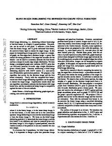
Figure 1. This figure shows a simple step edge image that has been blurred by two different PSF kernels: a 1D motion PSF with uniform speed (kernel A) and a 1D PSF with non-uniform speed (kernel B). These blurred images are transformed with a linear CRF (a)(c), and with a nonlinear CRF (b)(d). The 1D PSF and the 1D slice of intensity values are also shown. (e)-(h) show non-blind deconvolution results of (a)-(d) using Wiener filter. (i)-(l) show non-blind deconvolution results of (a)-(d) using an iterative re-weighting method [14] with sparsity regularization.

not consider the nonlinearity in the imaging process due to CRFs. The goal of radiometric calibration is to compute a CRF from a given set of images or a single image. The most accurate radiometric calibration algorithms use multiple images with different exposures [5, 7, 10, 18, 12]. Our work is more related to single-image based radiometric calibration techniques [16, 17, 21, 20, 30]. In [16], the CRF is computed by observing the color distributions of local edge regions: the CRF is computed as the mapping that transforms nonlinear distributions of edge colors into linear distributions. This idea is further extended to deal with a single gray-scale image using histograms of edge regions in [ 17]. In [30], a CRF is estimated by temporally mixing of a step edge within a single camera exposure by the linear motion blur of a calibration pattern. Unlike [30], however, our method deals with uncontrolled blurred images. To the best of our knowledge, there are only a handful of previous works that consider CRFs in the context of image deblurring. Examples include work by Fergus et al. [ 6], where images are first linearized by an inverse gammacorrection with γ = 2.2. Real world CRFs, however, are often drastically different from gamma curves [ 7, 15]. Another example by Lu et al. [18] involves reconstructing a high dynamic range image from a set of differently exposed and possibly motion blurred images. Recent work by Cho et al. [3] discussed nonlinear CRFs as a cause for artifacts in

deblurring, but provided little insight into why such artifacts arise. Their work suggested to avoid this by using a pre-calibrated CRF or the camera’s RAW output. While a pre-calibrated CRF is undoubtedly the optimal solution, the CRF may not always be available. Moreover, work by Chakrabarti et al. [2] suggests that a CRF may be scene dependent when the camera is in “ auto mode”. Recent work by Lin et al. [15] showed that the CRF for a given camera may vary for different camera picture styles (e.g., landscape, portrait, etc). Our work aims to provide more insight into the effect that CRFs have on the image deblurring process. In addition, we seek to provide a method to estimate a CRF from a blurred input image in the face of a missing or unreliable pre-calibrated CRF.

3. Effects of the CRF in image deblurring To focus our analysis, we follow previous work by assuming that the image noise is negligible (i.e., n ≈ 0 in Equation (2)) and that the PSF is spatially invariant.

3.1. Effects on PSF and image deconvolution We begin our analysis using synthetic examples shown in Figure 1. An image with three different intensity levels (Black, Gray, and White) is blurred with 1D motion PSFs with uniform speed (kernel A) and non-uniform speed (kernel B) to generate the observations in Figure 1 (a)(b) and

1

PSF θ

2 ge

marginal probability

ed

After CRF Re-mapping

ge

1

Before CRF Re-mapping

ed 0

0

CDF 1

Figure 2. This figure illustrates the problem when the image intensities are re-mapped according to different part of the camera response function. Two identical edge profiles at different intensity ranges are re-mapped to have different shapes.

θ

edge profile

Figure 4. This figure shows how the edge profile of a step edge in a motion blurred image is equal to the cumulative distribution function of the marginal probability of the motion blur kernel along the direction perpendicular to the edge.

icantly larger than the one with the linear CRF. The use of image regularization [14] helps to reduce the ringing artifacts, but the regularization is less effective in the case of a nonlinear CRF even with a very large regularization weight. Hence, the CRF plays a significant role in quality of the image deblurring.

3.2. Effects on PSF estimation

(a)

(b)

(c)

(d)

Figure 3. This figure shows examples of PSF kernels from several images with linear CRF (left columns) or nonlinear CRF (right columns). PSF kernels in the same row of (a)-(d) are from the same image with different estimated methods: (a) Fergus et al. [6]; (b) Shan et al. [23]; (c) Xu and Jia [31]; (d) Cho et al. [4].

Figure 1 (c)(d) respectively. A real CRF 1 is used to nonlinearly re-map the image intensity in Figure 1 (b)(d) after convolution. In this example, we can observe how the blur profiles of an image becomes spatially varying after the nonlinear re-mapping of image intensities even though the underlying motion PSF is spatially invariant. With a linear CRF, the blur profile from the black to gray region (first step edge) is the same as the blur profile from the gray to white region (second step edge) as shown in Figure 1 (a)(c). However, with a nonlinear CRF, the two blur profiles become different as shown in Figure 1 (b)(d). This is because the slope and the curvature of the CRF are different for different range of intensities. Figure 2 helps to illustrate this effect. To examine the effect that these cases have on image deblurring, we performed non-blind deconvolution on the synthetic images as shown in the second and third rows of Figure 1. The second row shows the results of Wiener filtering [29] while the third row shows the results of [14] with sparsity regularization. Without using any regularization, the deblurring results of both the linear and nonlinear CRF contain ringing artifacts due to the zero component of the PSF in the frequency domain. However, the magnitude of these ringing artifacts in the nonlinear CRF result is signif1 Pre-calibrated

CRF of a Cannon G5 camera in standard mode is used.

We also analyze the effects of a CRF on the PSF estimation by comparing the estimated PSF between a linear and nonlinear CRF. We show the estimated PSFs from Fergus et al. [6], Shan et al. [23], Xu and Jia [31] and Cho et al. [4] in Figure 3. The raw images from [4] were used for our testing purpose. Ideally, the CRF should only affect the relative intensity of a PSF, but the shape of a PSF should remain the same since the shape of the PSF describes the trajectory of motion causing the motion blur, and the intensity of the PSF describes the relative speed of the motion. However, as we can observe in Figure 3, the estimated PSFs are noticeably different, especially for the results from [6] and [23]. This is because both [6] and [23] use alternating optimization for their non-blind deconvolution. As previously discussed, the nonlinear CRF causes errors during the deconvolution process which in turn propagates the errors to the estimated PSF in an alternating optimization framework. The results from [31] and [4] contains less errors because they separate the process of PSF estimation and image deconvolution. However, the shape of the estimated PSF are still different. The method in [31] requires edge selection and sharpening, and the method in [4] requires edge profiles to be aligned. Since the nonlinear CRF alters the edge profiles in the blurred image, their estimated PSF also contains errors inherent from non-uniform edge profiles. Note that small errors in PSF estimation can causes significant artifacts in subsequent deconvolution.

4. CRF approximation from a blurred image In this section, we describe a method to estimate the CRF from one or more blurred images. To begin, we examine the relationship between the PSF and edge profiles in a blurred image under a linear CRF assumption. We then describe a

method to estimate the CRF based on this relationship using least-squares fitting assuming a known PSF. This method is then converted to a robust estimation of an unknown PSF and a CRF using rank minimization.

4.1. PSF and edge profiles We begin with the observation that the shape of a blur profile with the linear CRF resembles the shape of the cumulative distribution of the 1D PSF as shown in Figure 1 (a)(c). Our analysis is similar in fashion to that in [9] which used alpha mattes of blurred object to estimate the PSF. Our approach, however, works directly from the image intensities and requires no matting or object extraction. Instead, we only need to identify the step edges with homogeneous areas on both sides. For such edges, the shape of the blur profile is equal to the shape of the cumulative distribution of the 1D PSF. Consider a simple case where the original step edge has values [0, . . . , 0, 1, . . . , 1] and the values of the PSF is [α1 , α2 , . . . , αM ]. If the number of 0’s and 1’s are both larger than M , the blur after the motion blur profile M is equal to [α1 , α1 + α2 , . . . , i=1 αi ], which is the cumulative distribution of the 1D PSF. For any edges with intensities [I1 , I2 ], the value of the blur mprofile at m ∈ [1, . . . , M ] after the blur is equal to I 1 + i=1 αi (I2 − I1 ). In the case of a 2D PSF this observation still holds when the edge is a straight line. In this case, the 1D PSF becomes the marginal probability of the 2D PSF projected onto the line perpendicular to the edge direction as illustrated in Figure 4.

4.2. CRF approximation with a known PSF Considering that the shape of blurred edge profiles are equal to the shape of the cumulative distribution of the PSF 2 if the CRF is linear, if we are given the PSF, we can compute the CRF as follows:  2 E1  m M  g(Ij (m)) − lj  wj − αi argmin wj g(·) j=1 m=1 i=1  2 E2  M M   g(Ij (m)) − lj + wj − αi , (3) wj j=1 m=1 i=m where g(·) = f −1 (·) is the inverse CRF function, E 1 and E2 are the numbers of selected blurred edge profiles from dark to bright regions and from bright region to dark regions, respectively. The variables lj and wj are the minimum intensity value and the intensity range (intensity difference between the maximum and the minimum intensity values) of the blurred edge profiles after applying the inverse CRF. Blur profiles that span a wider intensity range are weighted more because 2 For

simplicity, we assume that the PSF is 1D, and it is well aligned with the edge orientation. If the PSF is 2D, we can compute the marginal probability of the PSF.

their wider dynamic range covers a larger portion of g(·), and therefore provide more information about the shape of g(·). We follow the method in [30] and model the inverse CRF g(·) using a polynomial of degree d = 5 with coefficients d ap , i.e., g(I) = p=0 ap I p . The optimization is subject to boundary constraints g(0) = 0 and g(1) = 1, and a monotonicity constraint that enforces the first derivative of g(·) to be non-negative. Our goal is to find the coefficients a p such that the following objective function is minimized: E1  M  wj argmin ap

j=1 m=1

+

E2  M 

 d p=0

wj  d

⎛



+λ1 ⎝a20 + +λ2

255 

 H

r=1

d 

ap Ij (m) − lj wj 2 ⎞

ap − 1



ap

p=0

2

M  − αi

2

i=m

⎠

p=0 d 

m  − αi i=1

p

p=0

wj

j=1 m=1

ap Ij (m)p − lj

r−1 255

p

 r p  − ,(4) 255

where H is the Heviside step function for enforcing the monotonicity constraint, i.e., H = 1 if g(r) < g(r − 1), or H = 0 otherwise. The weights are fixed to λ 1 = 100 and λ2 = 10, which control the boundary constraint and the monotonic constraint, respectively. The solution of Equation (4) can be obtained by a simplex search method of Lagarias et al. [11]3 .

4.3. CRF estimation with unknown PSF Using the cumulative distribution of the PSF can reliably estimate the CRF under ideal conditions. However, the PSF is usually unknown in practice. As we have studied in Section 3.2, nonlinear CRF affects the accuracy of the PSF estimation, which in turn will affect our CRF estimation described in Section 4.2. In this section, we introduce a CRF estimation method without explicitly computing the PSF. As previously discussed, we want to find an inverse response function g(·) that makes the blurred edge profiles have the same shape after applying the inverse CRF. This can be achieved by minimizing the distance between each blur profile to the average blur profile: argmin g(·)

E1  M 

+

j=1 m=1 3 fminsearch

2 g(Ij (m)) − lj − A1 (m) wj



2 g(Ij (m)) − lj − A2 (m) , (5) wj

wj

j=1 m=1 E2  M 



wj

function in Matlab.

 E 1 wk where A1 (m) = k=1 W g(Ik (m)) is the weighted avE1 erage blur profile, and W = l=1 wl is a normalization factor. Using the constraint in Equation (5), we can compute the CRF, however, this approach is unreliable not only because the constraint in Equation (5) is weaker than the constraint in Equation (3), but the nature of least-squares fitting is very sensitive to outliers. To avoid these problems, we generalize our method to robust estimation via rank minimization. Since the CRF of images from the same camera is the same, our generalized method can be extended to handle multiple motion blurred images which allow us to achieve accurate CRF estimation even without knowing the PSF. Recall that the edge profiles should have the same shape after applying the inverse CRF. This means that if the CRF is linear, the edge profiles are linearly dependent with each other, and hence the observation matrix of edge profiles form a rank-1 matrix for each group of edge profiles: ⎞ ⎛ ··· g(I1 (M )) − l1 g(I1 (1)) − l1 ⎟ ⎜ .. .. .. g(M)=⎝ ⎠ ,(6) . . . g(IE1 (1)) − lE1

···

g(IE1 (M )) − lE1

where M is length of edge profiles, and E 1 is the number of observed edge profiles grouped according to the orientation of edges. Now, we transform the problem into a rank minimization problem which finds a function g(·) that minimizes the rank of the observation matrix M of edge profiles. Since the CRF is the same for the whole image, we define our objective function for rank minimization as follow: arg min g(·)

K 

wk rank(g(Mk )),

(7)

k=1

where K is total number of observation matrix (total number of group of edge profiles), w k is a weight given to each observation matrix. We assign larger weight to the observation matrix that contains more edge profiles. Note that Equation (7) is also applicable to multiple images since the observation matrix are built individually for each edge orientation and for each input image. We evaluate the rank of matrix M by measuring the ratio of its singular values: argmin g(·)

K  k=1

Ek  σkj wk , σ j=2 k1

(8)

where σkj are the singular values of g(M) k . If the observation matrix is rank-1, only the first singular values is nonzero and hence minimizes Equation ( 8). In our experiments, we found that Equation (8) can be simplified to just measuring the ratio of the first two singular values: argmin g(·)

K  k=1

wk

σk2 . σk1

(9)

Combining the monotonic constraint, the boundary constraint and the polynomial function constraint from Equation (4), we obtain our final objective function: ⎛  d 2 ⎞ K   σk2 wk + λ1 ⎝a20 + ap − 1 ⎠ (10) argmin σk1 ap p=0 k=1  d  255  

r − 1 p r p  +λ2 H ap − . 255 255 r=1 p=0 Equation (10) can be solved effectively using nonlinear least-squares fitting4 .

4.4. Implementation issues for 2D PSF Our two proposed methods for CRF estimation are based on the 1D blur profile analysis. Since, in practice, PSFs are 2D in nature, we need to group image edges with similar orientation and select valid edge samples for building the observation matrix. We use the method in [4] to select the blurred edges. Method in [4] filters edges by only keeping high contrast straight-line edges. After we select valid edge profiles, we group the edge profiles according to edge orientations. In [4], edges were aligned according to the center of mass. In our case, however, to deal to the nonlinear CRF effects, alignment based on the center of mass is not reliable. We instead align the edge profiles by aligning the two end points of edges. Our method uses a nonlinear least-squares fitting for the rank minimization. This method can be sensitive to the initial estimation of the CRF. In our implementation, we use the average CRF profile from the database of response functions (DoRF) created by Grossberg and Nayar [8] as our initial guess. The DoRF database contains 201 measured functions which allows us to obtain a good local minima in practice.

5. Experimental results In this section, we evaluate the performance of our CRF estimation method using both synthetic and real examples. In the synthetic examples, we test our algorithm under different conditions in order to better understand the behaviors and the limitations of our method. In the real examples, we evaluate our method by comparing the amount of ringing artifacts with and without CRF intensity correction to demonstrate the effectiveness of our algorithm and the importance of CRF in the context of image deblurring.

5.1. Synthetic examples Figure 5 shows the performance of our CRF estimation under different conditions. We first test the effects of the intensity range of the blur profiles in Figure 5 (a). In a real 4 lsqnonlin

function in Matlab.

1

1

1

PSF

0

0

50

100

150

200

250

300

0

0

50

100

150

(a)

200

250

300

0

0

50

100

150

200

250

PSF

300

0.8

0

50

100

150

200

250

PSF

300

0.8

0

0.8

0.8

0.7

0.7

0.7

0.7

0.6

0.6

0.6

0.6

0.5

0.5

0.5

0.5

0.5

0.4

0.4

0.4

0.4

0.4

0.3

0.3

0.3

0.3

0.3

0.2

0.2

0.2

0.2

0.2

0.1

0.1

0.1

0.1

0.2

0.4

0.6

0.8

1

0

0

0.2

0.4

0.6

0.8

1

0

0

0.2

0.4

150

0.6

0.8

1

0

200

250

300

Ground Truth With known PSF (Eq. 4) With Observation Matrix (Eq. 6) & Rank Minimization (Eq. 10)

0.9

0.6

0

100

1

Ground Truth With known PSF (Eq. 4) With Observation Matrix (Eq. 6) & Rank Minimization (Eq. 10)

0.9

0.7

0

50

(e)

1

Ground Truth With known PSF (Eq. 4) With Observation Matrix (Eq. 6) & Rank Minimization (Eq. 10)

0.9

0

(d)

1

Ground Truth With known PSF (Eq. 4) With Observation Matrix (Eq. 6) & Rank Minimization (Eq. 10)

0.9

0

(c)

1

Ground Truth With known PSF (Eq. 4) With Observation Matrix (Eq. 6) & Rank Minimization (Eq. 10)

0.8

1

PSF

(b)

1 0.9

1

PSF

0.1 0

0.2

0.4

0.6

0.8

1

0

0

0.2

0.4

0.6

0.8

1

(f) (g) (h) (i) (j) Figure 5. We test the robustness of our CRF estimation method under different configurations. (a) Blur profiles with different intensity ranges, (b) edges in the original image contains mixed intensities (edge width is equal to 3 pixels), (c) Gaussian noise (σ = 0.02) is added according to Equation (2), (d) the union of intensity range of all blur profiles does not cover the whole CRF curve. (e) Blur profiles of (a), (b), (c), (d). The original image (black lines), the blurred image with linear CRF (red lines), and the blurred image with nonlinear CRF (blue lines) are shown on top of each figure in (a)-(d). (f)-(i) the corresponding estimated inverse CRF using our methods with (a)-(d). (j) the corresponding estimated inverse CRF with multiple images in (e).

application, it is uncommon that all edges will have a similar intensity range. These intensity range variations can potentially affect the estimated CRF as low dynamic range edges usually contain larger quantization errors. As shown in Figure 5 (f), our method is reasonably robust to these intensity range variations. Our method assumes that the original edges are step edges. In practice, there may be color mixing effect even for an edge that is considered as a sharp edge. In our experiments, we find that the performance of our approach degrades quickly if the step edge assumption is violated. However, as shown in Figure 5 (g), our approach is still effective if the color mixing effects is less than 3 pixel width given a PSF with size 15. The robustness of our method when edge color mixing is present depends on the size of PSF with our approach being more effective for larger PSFs. Noise is inevitable even when the ISO of a camera is high. We test the robustness of our method against image noise in Figure 5 (c). We add Gaussian noise to Equation (2) where the noise is added after the convolution process but before the CRF mapping. As can be observed in Figure 5 (h), the noise affects the accuracy of our method. In fact, using the model in Equation (2), we can observe that the noise has also captured some characteristics of the CRF. The magnitude of noise in the darker region is larger than the magnitude of noise in the brighter region. Such information may even be useful and combined into our framework to improve the performance of our algorithm as discussed in [20]. We test the sensitivity of our algorithm if the union of blur profiles does not cover the whole range of CRF. As we can be seen in Figure 5 (i), our method still gives reasonable estimations. This is because the polynomial and monotonic-

ity constraint assist in maintaining the shape of CRF. Note that having limited range of intensities will degrade the performance of all radiometric calibration methods. Finally, we show a result where we use all input images to estimate the CRF. As expected, more input images give a more accurate CRF estimation. Among all the synthetic experiments, we found that the performance of our method depends on the quality of the blur profiles and not only the quantity of observed blur profiles. For instance, a blur profile with a large motion covering a wide intensity range is better than the combination of blur profiles that cover only a portion of intensity range. When combining the observations from multiple images, our estimated CRF is more accurate as the mutual information from different images increase the robustness of our algorithm. The rank minimization also makes our algorithm less sensitive to outliers.

5.2. Real examples We test our method using real examples in Figure 6. Since the goal of this work is to understand the role of the CRF in the context of image deblurring, and hence to improve the performance of existing deblurring algorithm, we evaluate our method by comparing the amount of ringing artifacts in the deblurred image in addition to the accuracy of our estimated CRF. We estimate the inverse CRF using the method in Section 4.3. Although we can include the PSF information into our estimation, as discussed in Section 4.3, it is possible that the errors in the PSF would be propagated to the CRF. We therefore separate the CRF estimation step and the PSF estimation step. The accuracy of our estimated CRF for the real examples does not depend on the PSF estimation algo-

1

Ground Truth Our Estimated CRF with Single Image Our Estimated CRF with multiple Images Inverse Gamma-Correction

0.9 0.8 0.7 0.6 0.5 0.4 0.3 0.2 0.1 0

0

0.2

0.4

0.6

0.8

1

0.8

1

0.8

1

1

Ground Truth Our Estimated CRF with Single Image Our Estimated CRF with multiple Images Inverse Gamma-Correction

0.9 0.8 0.7 0.6 0.5 0.4 0.3 0.2 0.1 0

0

0.2

0.4

0.6

1

Ground Truth Our Estimated CRF with Single Image Our Estimated CRF with multiple Images Inverse Gamma-Correction

0.9 0.8 0.7 0.6 0.5 0.4 0.3 0.2 0.1 0

0

0.2

0.4

0.6

(a) (b) (c) (d) Figure 6. Our result with real examples: (a) input images; (b) estimated CRFs; (c) deblurred images with gamma correction; (d) deblurred images with CRF correction.

rithm. In our implementation, we choose the method in [ 31] to estimate the PSF and the method in [14] with sparsity regularization for deconvolution. Figure 6 show the results from the input image in (a) that is captured by Canon EOS 400D (first row) and a Nikon D90 DSLR (second and third rows) camera with a nonlinear CRF. The results in (b) are the estimated CRF using single and multiple images. The ground truth CRFs were computed by using method in [12] with calibration pattern. For reference, we have also show the inverse gamma-correction curve with γ equal to 2.2. This is the common method suggested by previous deblurring algorithm [ 6] when the CRF is nonlinear. Note the shape of inverse gamma-correction curve is very different from the shape of ground truth and our estimated CRF. We compare the results with gamma correction (γ = 2.2) and with our estimated CRF corrections in (c) and (d) respectively. As expected, our results with CRF corrections are better – not only do the deblurring results contain less artifacts, but the estimated PSFs are also more accurate after CRF correction.

sented an analysis on the role that nonlinear CRFs play in image deblurring. We showed that a nonlinear CRF can change a spatially invariant blur into one that is spatially varying. This caused notable ringing artifacts in the deconvolution process which cannot be completely ameliorated by image regularization. We also demonstrated how the nonlinear CRF adversely affects PSF estimation for several state-of-the-art techniques. In Section 4, we discussed how the shape of edge projections resemble the cumulative distribution function of 1D PSFs for linear CRFs. This observation was used to formulate two CRF estimation strategies for when the motion blur PSF kernel is known or not known. In the latter case, we showed how rank minimization can be used to provide a robust estimation. Experimental results in real examples demonstrated the importance of intensity linearization in the context of image deblurring. For future work we are interested to see if our approach can be extended to images with spatially varying motion blur such as camera rotational blur [27].

7. Acknowledgement 6. Discussion and summary This paper offers two contributions targeting image deblurring in the face of nonlinear CRFs. First, we have pre-

This research is supported in part by the MKE, Korea and Microsoft Research, under the IT/SW Creative Research Program supervised by the NIPA (NIPA- 2011-C1810-

1102-0014), the National Research Foundation (NRF) of Korea (2011-0013349), and Singapore Academic Research Fund (AcRF) Tier 1 FRC grant (Project No. R-252-000423-112).

References [1] M. Ben-Ezra and S. Nayar. Motion-based Motion Deblurring. IEEE Trans. PAMI, 26(6):689–698, Jun 2004. 1 [2] A. Chakrabarti, D. Scharstein, and T. Zickler. ”an empirical camera model for internet color vision”. In BMCV, 2009. 2 [3] S. Cho, J. Wang, and S. Lee. Handling Outliers in Non-blind Image Deconvolution. In ICCV, 2011. 2 [4] T.-S. Cho, S. Paris, B. Freeman, and B. Horn. Blur kernel estimation using the radon transform. In CVPR, 2011. 3, 5 [5] P. Debevec and J. Malik. Recovering high dynamic range radiance maps from photographs. In ACM SIGGRAPH, 1997. 2 [6] R. Fergus, B. Singh, A. Hertzmann, S. T. Roweis, and W. T. Freeman. Removing camera shake from a single photograph. ACM Trans. Graph., 25(3), 2006. 1, 2, 3, 7 [7] M. Grossberg and S. Nayar. Modeling the space of camera response functions. IEEE Trans. PAMI, 26(10), 2004. 1, 2 [8] M. D. Grossberg and S. K. Nayar. What is the space of camera response functions? CVPR, 2003. 5 [9] J. Jia. Single image motion deblurring using transparency. In CVPR, 2007. 1, 4 [10] S. J. Kim and M. Pollefeys. Robust radiometric calibration and vignetting correction. IEEE Trans. PAMI, 30(4), 2008. 2 [11] J. Lagarias, J. Reeds, M. Wright, and P. Wright. Convergence properties of the nelder-mead simplex method in low dimensions. SIAM Journal of Optimization, 9(1):112–147, 1998. 4 [12] J.-Y. Lee, B. Shi, Y. Matsushita, I. Kweon, and K. Ikeuchi. Radiometric calibration by transform invariant low-rank structure. In CVPR, 2011. 2, 7 [13] A. Levin. Blind motion deblurring using image statistics. In NIPS, 2006. 1 [14] A. Levin, R. Fergus, F. Durand, and W. T. Freeman. Image and depth from a conventional camera with a coded aperture. ACM Trans. Graph., 26(3), 2007. 2, 3, 7 [15] H. Lin, S. J. Kim, S. Susstrunk, and M. S. Brown. Revisiting radiometric calibration for color computer vision. In ICCV, 2011. 2

[16] S. Lin, J. Gu, S. Yamazaki, and H.-Y. Shum. Radiometric calibration from a single image. In CVPR, 2004. 2 [17] S. Lin and L. Zhang. Determining the radiometric response function from a single grayscale image. In CVPR, 2005. 1, 2 [18] P.-Y. Lu, T.-H. Huang, M.-S. Wu, Y.-T. Cheng, and Y.Y. Chuang. High dynamic range image reconstruction from hand-held cameras. In CVPR, 2009. 2 [19] L. Lucy. An iterative technique for the rectification of observed distributions. Astron. J., 79, 1974. 1 [20] Y. Matsushita and S. Lin. Radiometric calibration from noise distributions. In CVPR, 2007. 2, 6 [21] T.-T. Ng, S.-F. Chang, and M.-P. Tsui. Using geometry invariants for camera response function estimation. In CVPR, 2007. 2 [22] W. Richardson. Bayesian-based iterative method of image restoration. J. Opt. Soc. Am., 62(1), 1972. 1 [23] Q. Shan, J. Jia, and A. Agarwala. High-quality motion deblurring from a single image. ACM Trans. Graph., 2008. 3 [24] Y.-W. Tai, H. Du, M. Brown, and S. Lin. Image/video deblurring using a hybrid camera. In CVPR, 2008. 1 [25] Y.-W. Tai, H. Du, M. S. Brown, and S. Lin. Correction of spatially varying image and video motion blur using a hybrid camera. IEEE Trans. PAMI, 32(6):1012– 1028, 2010. 1 [26] Y.-W. Tai, N. Kong, S. Lin, and S. Shin. Coded exposure imaging for projective motion deblurring. In CVPR, 2010. 1 [27] Y.-W. Tai, P. Tan, and M. Brown. Richardson-lucy deblurring for scenes under projective motion path. IEEE Trans. PAMI, 33(8):1603–1618, 2011. 1, 7 [28] O. Whyte, J. Sivic, A. Zisserman, and J. Ponce. Nonuniform deblurring for shaken images. In CVPR, 2010. 1 [29] N. Wiener. Extrapolation, interpolation, and smoothing of stationary time series. New York: Wiley, 1949. 1, 3 [30] B. Wilburn, H. Xu, and Y. Matsushita. Radiometric calibration using temporal irradiance mixtures. In CVPR, 2008. 2, 4 [31] L. Xu and J. Jia. Two-phase kernel estimation for robust motion deblurring. In ECCV, 2010. 3, 7 [32] L. Yuan, J. Sun, L. Quan, and H. Shum. Image deblurring with blurred/noisy image pairs. ACM Trans. Graph., 26(3), 2007. 1