Tolerance of noise A related issue for data-based reduction methods is the ... Web of Science for the terms listed above, which turns up more than 30,000 references ... where Var(yâ¢j ) denotes the sample variance of the jth component of a set of vectors yi ..... position [Stewart, 1993] into a common theoretical framework to aid ...
Nonlinear Dimensionality Reduction
arXiv:0901.0537v1 [physics.ao-ph] 2 Jan 2009
Methods in Climate Data Analysis
Ian Ross
A dissertation submitted to the University of Bristol in accordance with the requirements of the degree of Doctor of Philosophy in the Faculty of Science School of Geographical Sciences University of Bristol September 2008 ca. 80,000 words
© Ian Ross Some Rights Reserved, 2008 Except where otherwise noted, this work is licensed under http://creativecommons.org/licenses/by/3.0/
Abstract
Linear dimensionality reduction techniques, notably principal component analysis, are widely used in climate data analysis as a means to aid in the interpretation of datasets of high dimensionality. These linear methods may not be appropriate for the analysis of data arising from nonlinear processes occurring in the climate system. Numerous techniques for nonlinear dimensionality reduction have been developed recently that may provide a potentially useful tool for the identification of low-dimensional manifolds in climate data sets arising from nonlinear dynamics. In this thesis I apply three such techniques to the study of El Niño/Southern Oscillation variability in tropical Pacific sea surface temperatures and thermocline depth, comparing observational data with simulations from coupled atmosphereocean general circulation models from the CMIP3 multi-model ensemble. The three methods used here are a nonlinear principal component analysis (NLPCA) approach based on neural networks, the Isomap isometric mapping algorithm, and Hessian locally linear embedding. I use these three methods to examine El Niño variability in the different data sets and assess the suitability of these nonlinear dimensionality reduction approaches for climate data analysis. I conclude that although, for the application presented here, analysis using NLPCA, Isomap and Hessian locally linear embedding does not provide additional information beyond that already provided by principal component analysis, these methods are effective tools for exploratory data analysis.
iii
Author’s Declaration
I declare that the work in this dissertation was carried out in accordance with the Regulations of the University of Bristol. The material presented here is the result of my own independent research performed at the University of Bristol, School of Geographical Sciences, between October 2005 and September 2008, and no part of the dissertation has been submitted for any other academic award. Sections of Chapters 3, 4 and 5 and all of Chapter 7 have previously appeared as: I. Ross, P. J. Valdes and S. Wiggins. ENSO dynamics in current climate models: an investigation using nonlinear dimensionality reduction. Nonlin. Processes Geophys., 15(2):339–363, April 2008. Any opinions expressed in this thesis are those of the author.
Ian Ross September 2008
v
Acknowledgments
Many thanks to my supervisors, Paul Valdes and Steve Wiggins. Paul, first of all, gave me a job and provided a nurturing and congenial environment, in the form of the BRIDGE group. Paul’s easy-going leadership really set the tone for BRIDGE (“field trips” that consist of a weekend camping and surfing in Devon, anyone?), which ended up being a very productive arrangement for everyone concerned. I’ve certainly enjoyed being part of that and the group will be something I’ll miss a lot when I leave Bristol. As for Steve, during the three years of my Ph.D., we missed just a handful of our weekly meetings due to his absence or other engagements. For someone covering head of department responsibilities while maintaining an active research programme, that’s an extraordinary level of commitment, one for which I am very grateful. The only thing that (slightly) tempers this gratitude is Steve’s habit of sending emails in the dead of night with wads of papers attached to them, all with the comment “You really should know about this stuff...”. As a result of Steve’s “encouragement”, I’ve probably read about five times as much as I otherwise would have done. I even enjoyed some of it. Of the other BRIDGE-ites, special mention has to go to Rupes (for always refusing to understand things in the most enlightening fashion possible), Dan (“I trust David Blunkett!”), Gethin (a boy from Wales more interested in computers than sheep) and Rachel (her door is always open, she’s always ready for a chat, and she lives at the bottom of the steepest hill in Somerset). Also, apologies to anyone who’s had to give a group seminar with me in the front row heckling (that’s nearly everyone!). This is a thesis about climate data analysis, so we need some climate data. I’ve used data from the NCEP atmospheric and ocean reanalyses, both truly excellent resources, I’ve used the NOAA ERSST v2 data set, and I’ve used GCM simulations archived for the IPCC Fourth Assessment Report. There’s a blurb that goes with the IPCC data: “I acknowledge the modelling groups, the Program for Climate Model Diagnosis and Intercomparison (PCMDI) and the WCRP’s Working Group on Coupled Modelling (WGCM) for their roles in making available the WCRP CMIP3 multi-model data set. Support for this data set is provided by the Office of Science, U.S. Department of Energy”. Those official words don’t capture just how useful these multi-model ensemble databases are and what a job it is to organise them. All kudos to the people involved! On another official note, I should mention that my Ph.D. work was funded by an e-Science studentship from NERC, number NER/S/G/2005/13913. Finally, of course, an enormous thank you to Rita. She lives with me, shares her life with vii
ACKNOWLEDGMENTS
me, sometimes works with me, even puts up with my “jokes”, and yet through all of this, she maintains the sunniest of dispositions, the happiest of smiles. As anyone who knows me will attest, this must mean that she is a very angel. We’ve had a lot of fun over the last four and a half years, including some things that were more “fun” than fun (the completion of two Ph.D.s, broken collarbones, invisible fishbones, immigration anxieties), but some that were absolute unalloyed FUN (holidays in Ireland, Greece, even Austria, and every everyday day). I am absolutely sure that we will have many years more. Life is good, and the reason is Rita.
viii
Table of Contents
Abstract
iii
Author’s Declaration
v
Acknowledgments
vii
List of Tables
xiii
List of Figures
xv
1 Introduction
3
2 Overview of Nonlinear Dimensionality Reduction
7
2.1 Definitions of dimensionality . . . . . . . . . . . . . . . . . . . . . . . . . . . . . .
8
2.2 Dimensionality reduction . . . . . . . . . . . . . . . . . . . . . . . . . . . . . . . . 14 2.3 Classifying dimensionality reduction methods . . . . . . . . . . . . . . . . . . . . 17 2.4 Linear methods . . . . . . . . . . . . . . . . . . . . . . . . . . . . . . . . . . . . . . 23 2.4.1 Principal component analysis . . . . . . . . . . . . . . . . . . . . . . . . . 24 2.4.2 Multidimensional scaling . . . . . . . . . . . . . . . . . . . . . . . . . . . . 30 2.4.3 Spectral methods . . . . . . . . . . . . . . . . . . . . . . . . . . . . . . . . . 30 2.4.4 Random projections . . . . . . . . . . . . . . . . . . . . . . . . . . . . . . . 31 2.5 Nonlinear methods . . . . . . . . . . . . . . . . . . . . . . . . . . . . . . . . . . . . 31 2.5.1 Differential geometry methods . . . . . . . . . . . . . . . . . . . . . . . . . 32 2.5.2 Kernel methods . . . . . . . . . . . . . . . . . . . . . . . . . . . . . . . . . . 42 2.5.3 Neural network methods . . . . . . . . . . . . . . . . . . . . . . . . . . . . 42 2.5.4 Spectral graph theory methods . . . . . . . . . . . . . . . . . . . . . . . . . 45 2.5.5 Computational topology . . . . . . . . . . . . . . . . . . . . . . . . . . . . . 47 2.5.6 Miscellaneous geometrical/statistical methods . . . . . . . . . . . . . . . 51 2.5.7 Out-of-sample extensions . . . . . . . . . . . . . . . . . . . . . . . . . . . . 54 2.6 Discussion . . . . . . . . . . . . . . . . . . . . . . . . . . . . . . . . . . . . . . . . . 55 3 Data and Models
57
3.1 Observational data . . . . . . . . . . . . . . . . . . . . . . . . . . . . . . . . . . . . 57 3.1.1 Sea surface temperature . . . . . . . . . . . . . . . . . . . . . . . . . . . . . 57 3.1.2 Thermocline depth and warm water volume . . . . . . . . . . . . . . . . . 58 ix
TABLE OF CONTENTS
3.2 The CMIP3 models . . . . . . . . . . . . . . . . . . . . . . . . . . . . . . . . . . . . 59 3.3 Geometrical test data sets . . . . . . . . . . . . . . . . . . . . . . . . . . . . . . . . 60 4 The El Niño/Southern Oscillation
65
4.1 Tropical Pacific climatology . . . . . . . . . . . . . . . . . . . . . . . . . . . . . . . 65 4.2 ENSO phenomenology . . . . . . . . . . . . . . . . . . . . . . . . . . . . . . . . . . 67 4.3 ENSO mechanisms . . . . . . . . . . . . . . . . . . . . . . . . . . . . . . . . . . . . 69 4.4 Modelling ENSO . . . . . . . . . . . . . . . . . . . . . . . . . . . . . . . . . . . . . . 73 4.4.1 General circulation models . . . . . . . . . . . . . . . . . . . . . . . . . . . 74 4.4.2 Statistical models . . . . . . . . . . . . . . . . . . . . . . . . . . . . . . . . . 76 4.4.3 Intermediate complexity models . . . . . . . . . . . . . . . . . . . . . . . . 77 4.4.4 Conceptual models . . . . . . . . . . . . . . . . . . . . . . . . . . . . . . . . 78 4.5 Previous applications of nonlinear dimensionality reduction to ENSO . . . . . . 84 5 Tropical Pacific Variability in Observations and the CMIP3 Models
87
5.1 Equatorial Pacific sea surface temperature . . . . . . . . . . . . . . . . . . . . . . 87 5.1.1 Basic equatorial Pacific SST variability . . . . . . . . . . . . . . . . . . . . 87 5.1.2 Principal component analysis of SST data . . . . . . . . . . . . . . . . . . 89 5.1.3 Asymmetry of SST variability . . . . . . . . . . . . . . . . . . . . . . . . . . 94 5.2 Equatorial Pacific thermocline depth . . . . . . . . . . . . . . . . . . . . . . . . . 97 5.2.1 Comparison of thermocline calculation methods . . . . . . . . . . . . . . 97 5.2.2 Principal component analysis of thermocline data . . . . . . . . . . . . . 100 5.3 Equatorial Pacific warm water volume . . . . . . . . . . . . . . . . . . . . . . . . . 103 5.3.1 Warm water volume calculation methods . . . . . . . . . . . . . . . . . . 103 5.3.2 NINO3 SST index/warm water volume phasing . . . . . . . . . . . . . . . 104 6 Nonlinear Principal Component Analysis
107
6.1 Description of method . . . . . . . . . . . . . . . . . . . . . . . . . . . . . . . . . . 107 6.1.1 Extension of ideas from PCA to a nonlinear setting . . . . . . . . . . . . . 107 6.1.2 Auto-associative neural networks . . . . . . . . . . . . . . . . . . . . . . . 108 6.1.3 Model fitting considerations . . . . . . . . . . . . . . . . . . . . . . . . . . 111 6.2 Application to test data sets . . . . . . . . . . . . . . . . . . . . . . . . . . . . . . . 118 6.3 Previous applications in climate data analysis . . . . . . . . . . . . . . . . . . . . 125 6.4 Application to analysis of Pacific SSTs . . . . . . . . . . . . . . . . . . . . . . . . . 127 6.4.1 SST NLPCA mode 1 . . . . . . . . . . . . . . . . . . . . . . . . . . . . . . . . 127 6.4.2 SST NLPCA mode 2 . . . . . . . . . . . . . . . . . . . . . . . . . . . . . . . . 140 6.4.3 Nonmodal 2-D NLPCA analysis . . . . . . . . . . . . . . . . . . . . . . . . . 148 6.5 Application to analysis of Pacific thermocline variability . . . . . . . . . . . . . . 151 6.6 Discussion and conclusions . . . . . . . . . . . . . . . . . . . . . . . . . . . . . . . 167 x
TABLE OF CONTENTS
7 Isomap
175
7.1 Description of method . . . . . . . . . . . . . . . . . . . . . . . . . . . . . . . . . . 175 7.1.1 Geodesic approximation . . . . . . . . . . . . . . . . . . . . . . . . . . . . . 175 7.1.2 Multidimensional scaling . . . . . . . . . . . . . . . . . . . . . . . . . . . . 176 7.1.3 Computational complexity . . . . . . . . . . . . . . . . . . . . . . . . . . . 178 7.2 Application to test data sets . . . . . . . . . . . . . . . . . . . . . . . . . . . . . . . 179 7.3 Isomap sensitivity . . . . . . . . . . . . . . . . . . . . . . . . . . . . . . . . . . . . . 180 7.4 Previous applications in climate data analysis . . . . . . . . . . . . . . . . . . . . 183 7.5 Application to analysis of Pacific SSTs . . . . . . . . . . . . . . . . . . . . . . . . . 183 7.5.1 Analysis for raw SSTs . . . . . . . . . . . . . . . . . . . . . . . . . . . . . . . 183 7.5.2 Analysis for SST anomalies . . . . . . . . . . . . . . . . . . . . . . . . . . . 192 7.6 Discussion and conclusions . . . . . . . . . . . . . . . . . . . . . . . . . . . . . . . 194 7.7 Rotation of Isomap components . . . . . . . . . . . . . . . . . . . . . . . . . . . . 197 7.7.1 Three-dimensional case . . . . . . . . . . . . . . . . . . . . . . . . . . . . . 198 7.7.2 Four-dimensional case . . . . . . . . . . . . . . . . . . . . . . . . . . . . . . 200 8 Hessian Locally Linear Embedding
203
8.1 Description of method . . . . . . . . . . . . . . . . . . . . . . . . . . . . . . . . . . 203 8.2 Application to test data sets . . . . . . . . . . . . . . . . . . . . . . . . . . . . . . . 206 8.3 Hessian LLE sensitivity . . . . . . . . . . . . . . . . . . . . . . . . . . . . . . . . . . 208 8.4 Application to analysis of Pacific SSTs . . . . . . . . . . . . . . . . . . . . . . . . . 212 8.5 Discussion and conclusions . . . . . . . . . . . . . . . . . . . . . . . . . . . . . . . 219 9 Summary and Future Work
223
Table of Notation
227
Glossary
229
Bibliography
233
xi
List of Tables
2.1 Table of dimensionality reduction methods . . . . . . . . . . . . . . . . . . . . . 18 3.1 Models used in this study . . . . . . . . . . . . . . . . . . . . . . . . . . . . . . . . 61 5.1 El Niño/La Niña asymmetry measures . . . . . . . . . . . . . . . . . . . . . . . . . 96 5.2 Z20 /Zgrad differences in WWV region . . . . . . . . . . . . . . . . . . . . . . . . . 99 5.3 Z20 /Zgrad WWV anomaly time series correlation values . . . . . . . . . . . . . . . 104 6.1 Parameter counts for NLPCA network architectures . . . . . . . . . . . . . . . . . 111 6.2 NLPCA SST mode 1 error and variance comparison . . . . . . . . . . . . . . . . . 129 6.3 SST mode explained variance fractions . . . . . . . . . . . . . . . . . . . . . . . . 142 6.4 NLPCA thermocline error and variance comparison . . . . . . . . . . . . . . . . 154 6.5 NLPCA α1 and α2 correlations . . . . . . . . . . . . . . . . . . . . . . . . . . . . . 169 7.1 Isomap dimensionality estimates for SST data . . . . . . . . . . . . . . . . . . . . 186 7.2 Correlation between NINO3 SST and WWV and Isomap components . . . . . . 190 8.1 Correlation between NINO3 SST index and Hessian LLE component . . . . . . 221
xiii
List of Figures
2.1 Lorenz attractor . . . . . . . . . . . . . . . . . . . . . . . . . . . . . . . . . . . . . . 14 2.2 RNC method . . . . . . . . . . . . . . . . . . . . . . . . . . . . . . . . . . . . . . . . 37 2.3 RML method . . . . . . . . . . . . . . . . . . . . . . . . . . . . . . . . . . . . . . . . 40 2.4 Self-organising map . . . . . . . . . . . . . . . . . . . . . . . . . . . . . . . . . . . 43 2.5 Simplicial homology example . . . . . . . . . . . . . . . . . . . . . . . . . . . . . . 49 2.6 Homology examples . . . . . . . . . . . . . . . . . . . . . . . . . . . . . . . . . . . 50 3.1 ERSST v2 SST wavelet power spectrum . . . . . . . . . . . . . . . . . . . . . . . . 58 3.2 Three-dimensional views of geometrical test data sets . . . . . . . . . . . . . . . 62 4.1 Mean climatological SST, thermocline and wind state of equatorial Pacific . . . 66 4.2 Walker circulation . . . . . . . . . . . . . . . . . . . . . . . . . . . . . . . . . . . . . 67 4.3 El Niño conditions in equatorial Pacific . . . . . . . . . . . . . . . . . . . . . . . . 68 4.4 La Niña conditions in equatorial Pacific . . . . . . . . . . . . . . . . . . . . . . . . 69 4.5 Cartoon view of ENSO cycle . . . . . . . . . . . . . . . . . . . . . . . . . . . . . . . 71 5.1 Equatorial Pacific climatological mean SST and annual SST standard deviation 88 5.2 NINO3 SST index power spectra . . . . . . . . . . . . . . . . . . . . . . . . . . . . 90 5.3 Equatorial Pacific SST EOFs . . . . . . . . . . . . . . . . . . . . . . . . . . . . . . . 91 5.4 Equatorial Pacific SST principal component scatter plots . . . . . . . . . . . . . 94 5.5 Seasonal variability of Zgrad thermocline depths . . . . . . . . . . . . . . . . . . . 98 5.6 Equatorial Pacific thermocline depth EOFs . . . . . . . . . . . . . . . . . . . . . . 101 5.7 Equatorial Pacific thermocline depth principal component scatter plots . . . . 102 5.8 NINO3 SST index/WWV phase plots . . . . . . . . . . . . . . . . . . . . . . . . . . 105 6.1 NLPCA neural network architecture . . . . . . . . . . . . . . . . . . . . . . . . . . 110 6.2 NLPCA reductions of geometrical test data sets . . . . . . . . . . . . . . . . . . . 119 6.3 NLPCA reconstructions of geometrical test data sets . . . . . . . . . . . . . . . . 121 6.4 NLPCA spiral example reconstructions . . . . . . . . . . . . . . . . . . . . . . . . 123 6.5 NLPCA spiral example error histogram . . . . . . . . . . . . . . . . . . . . . . . . 124 6.6 ERSST NLPCA SST mode 1 reconstruction . . . . . . . . . . . . . . . . . . . . . . 131 6.7 ERSST NLPCA SST mode 1 spatial patterns . . . . . . . . . . . . . . . . . . . . . . 133 6.8 ERSST NLPCA SST mode 1 error statistics . . . . . . . . . . . . . . . . . . . . . . . 133 xv
LIST OF FIGURES
6.9 CGCM3.1(T63) NLPCA SST mode 1 reconstruction . . . . . . . . . . . . . . . . . 136 6.10 CGCM3.1(T63) NLPCA SST mode 1 spatial patterns . . . . . . . . . . . . . . . . . 136 6.11 CNRM-CM3 NLPCA SST mode 1 reconstruction . . . . . . . . . . . . . . . . . . . 137 6.12 ECHO-G NLPCA SST mode 1 reconstruction . . . . . . . . . . . . . . . . . . . . . 137 6.13 GFDL-CM2.1 NLPCA SST mode 1 reconstruction . . . . . . . . . . . . . . . . . . 138 6.14 CNRM-CM3 NLPCA SST mode 1 spatial patterns . . . . . . . . . . . . . . . . . . 139 6.15 ECHO-G NLPCA SST mode 1 spatial patterns . . . . . . . . . . . . . . . . . . . . 139 6.16 GFDL-CM2.1 NLPCA SST mode 1 spatial patterns . . . . . . . . . . . . . . . . . . 140 6.17 UKMO-HadCM3 NLPCA SST mode 1 reconstruction . . . . . . . . . . . . . . . . 141 6.18 UKMO-HadCM3 NLPCA SST mode 1 spatial patterns . . . . . . . . . . . . . . . . 141 6.19 ERSST NLPCA SST mode 2 reconstruction . . . . . . . . . . . . . . . . . . . . . . 143 6.20 ERSST NLPCA α2 time series . . . . . . . . . . . . . . . . . . . . . . . . . . . . . . 144 6.21 ERSST NLPCA SST mode 2 spatial patterns . . . . . . . . . . . . . . . . . . . . . . 145 6.22 Strong ENSO events in ERSST data and NLPCA SST mode 2 . . . . . . . . . . . . 145 6.23 CNRM-CM3 NLPCA SST mode 2 reconstruction . . . . . . . . . . . . . . . . . . . 147 6.24 ECHO-G NLPCA SST mode 2 reconstruction . . . . . . . . . . . . . . . . . . . . . 147 6.25 GFDL-CM2.1 NLPCA SST mode 2 reconstruction . . . . . . . . . . . . . . . . . . 148 6.26 CNRM-CM3 NLPCA SST mode 2 spatial patterns . . . . . . . . . . . . . . . . . . 149 6.27 ECHO-G NLPCA SST mode 2 spatial patterns . . . . . . . . . . . . . . . . . . . . 149 6.28 GFDL-CM2.1 NLPCA SST mode 2 spatial patterns . . . . . . . . . . . . . . . . . . 149 6.29 ERSST NLPCA SST nonmodal reconstruction . . . . . . . . . . . . . . . . . . . . 150 6.30 CNRM-CM3 NLPCA SST nonmodal reconstruction . . . . . . . . . . . . . . . . . 152 6.31 NCEP GODAS NLPCA thermocline depth mode reconstruction . . . . . . . . . . 155 6.32 NLPCA thermocline depth decimation reconstruction . . . . . . . . . . . . . . . 157 6.33 NCEP GODAS NLPCA thermocline depth mode spatial patterns . . . . . . . . . 160 6.34 NCEP GODAS thermocline depth variation schematic . . . . . . . . . . . . . . . 161 6.35 CGCM3.1(T63) NLPCA thermocline depth mode reconstructions . . . . . . . . 163 6.36 CCSM3 NLPCA thermocline depth mode reconstructions . . . . . . . . . . . . . 164 6.37 FGOALS-g1.0 NLPCA thermocline depth mode reconstructions . . . . . . . . . 165 6.38 FGOALS-g1.0 NLPCA thermocline depth mode spatial patterns . . . . . . . . . . 166 6.39 ECHO-G NLPCA thermocline depth mode reconstructions . . . . . . . . . . . . 168 6.40 ECHO-G NLPCA thermocline depth mode spatial patterns . . . . . . . . . . . . 168 7.1 Isomap reductions of geometrical test data sets . . . . . . . . . . . . . . . . . . . 179 7.2 Isomap eigenvalue convergence: Swiss roll . . . . . . . . . . . . . . . . . . . . . . 181 7.3 Isomap eigenvalue convergence: tropical Pacific raw SSTs . . . . . . . . . . . . . 185 7.4 Three-dimensional Isomap embeddings . . . . . . . . . . . . . . . . . . . . . . . 188 7.5 NINO3 SST index and Isomap rotated component #3 time series . . . . . . . . . 189 7.6 Isomap eigenvalue convergence: SST anomalies . . . . . . . . . . . . . . . . . . . 193 7.7 Isomap component rotation . . . . . . . . . . . . . . . . . . . . . . . . . . . . . . 198 7.8 Isomap component rotation power spectra . . . . . . . . . . . . . . . . . . . . . . 200 xvi
LIST OF FIGURES
8.1 Hessian LLE reductions of geometrical test data sets . . . . . . . . . . . . . . . . 207 8.2 Hessian LLE sensitivity (no noise) . . . . . . . . . . . . . . . . . . . . . . . . . . . 209 8.3 Hessian LLE sensitivity (with noise) . . . . . . . . . . . . . . . . . . . . . . . . . . 210 8.4 Hessian LLE eigenvalue convergence: tropical Pacific SSTs . . . . . . . . . . . . 215 8.5 Three-dimensional Hessian LLE embedding for ERSST data . . . . . . . . . . . . 216 8.6 Three-dimensional Hessian LLE embedding for model SST data . . . . . . . . . 218 8.7 NINO3 SST index and Hessian LLE rotated component #3 time series . . . . . . 220
1
1
Introduction
Recent advances in observational and modelling technology have led to a situation in climate science that would have been unthinkable even a few years ago. Our problem? We have too much data! Satellite instruments and improved in situ monitoring networks observe variations in the climate system in unprecedented detail, while modern general circulation models (GCMs) simulate atmospheric, ocean and land surface processes at high spatial and temporal resolution. New methods and novel tools are needed to analyse the resulting glut of data. The problem is not simply the quantity of data, but that the data is represented as points in high-dimensional space, recording many simultaneous measurements. As an example, consider an atmospheric GCM that outputs a time series of geopotential height on several pressure levels. Each entry in this time series can be viewed as a single vector in Rm (R is the real numbers1 , and Rm is m-dimensional Euclidean space), where m is the number of spatial points in the model grid. For the UK Met Office HadCM3 model [Gordon et al., 2000], m = 133,152, representing a 96 × 73 horizontal grid with horizontal spatial resolution of 3.75◦ × 2.5◦ (longitude × latitude), with 19 vertical levels through the atmosphere. Collecting data on only three pressure levels (850 hPa2 , 500 hPa and 250 hPa, say, for a view of the lower, middle and upper troposphere), one still has m = 21,024. Thinking of such a model as a dynamical system, high-dimensional data of this type is difficult to interpret. Although two-dimensional geographical maps of geopotential height can be plotted on a single pressure level at a single time, this view is not appropriate for considering the dynamics of the system. To do this, the whole state of the model at a given timestep should be considered as a single point in the phase space Rm . The modern dynamical systems approach then considers evolution of the system as controlled by geometrical structures in phase space, such as periodic orbits, saddle points, and so on [Wiggins, 2003]. However, our situation is far from hopeless. It is a commonplace of observational meteorology and climatology that the evolution of the atmosphere and ocean is characterised by recognisable and recurrent coherent structures, such as synoptic weather systems in the at1 References to definitions of all non-standard notation can be found in the table of notation on page 227. 2 1 hPa = 100 Pa. This is a convenient unit for measurement of atmospheric pressure — sea level pressure is
around 1000 hPa, while 500 hPa represents a vertical level approximately half-way through the atmosphere, in terms of mass.
3
CHAPTER 1. INTRODUCTION
mosphere or mesoscale eddies in the ocean. The existence of these coherent structures represents a coupling between many individual degrees of freedom, couplings that persist for extended periods of time. This coherent behaviour leads to the hope that it may be possible to derive a simplified representation of the evolution of the atmosphere or ocean, eliminating degrees of freedom that are in some sense “uninteresting”, to concentrate on degrees of freedom that capture the large-scale coherent structures. This simplification represents a reduction of the dimensionality of the system: we go from our original high-dimensional representation including all of the degrees of freedom of the system to a lower-dimensional representation capturing the essential features of interest. Some encouragement for the project of constructing lower-dimensional representations of phenomena of interest in the climate system can be drawn from results in the rigorous functional analysis of partial differential equations (PDEs). Here, the long term behaviour of these infinite dimensional systems is found to be confined to a finite dimensional global attractor [Robinson, 1995]. In some cases, it can be proven that this attractor is embedded in a finite dimensional manifold, called the inertial manifold of the system. In this case, the long term dynamics of the infinite dimensional PDE system is rigorously equivalent to a finite dimensional system of ordinary differential equations describing a flow on the inertial manifold. Bounds on the dimensionality of the inertial manifold can sometimes be derived in terms of system parameters. While these results are both theoretically appealing and consonant with our intuitive notions of long term coherent behaviour in fluid systems, they are of relatively limited practical applicability. The bounds on attractor and inertial manifold dimension are typically very high, and the existence of inertial manifolds has only been proven for a restricted set of problems, a set excluding most of the equations of interest in applications to geophysical fluids and the climate system [Foias et al., 2001]. Another source of encouragement in the project of dimensionality reduction for climate dynamics lies in empirical observations of coherent structures in other fluid flows and, more generally, the existence of coherent dissipative structures for a wide range of nonlinear partial differential equation systems [Cross and Hohenberg, 1993]. The presence of these coherent patterns is a strong indication that aspects of the behaviour of these systems may be represented by an effective low-dimensional model. In this thesis, I report on the application of a number of methods of dimensionality reduction to a problem in climate data analysis, namely the study of interannual tropical Pacific climate variability and the El Niño/Southern Oscillation (ENSO). This problem is approached in the context of an inter-model comparison using the World Climate Research Programme’s (WCRP’s) Coupled Model Intercomparison Project phase 3 (CMIP3) multimodel data set. The primary goal here is to explore the applicability of some nonlinear dimensionality reduction methods to a relatively well understood problem in climate data analysis. It is unlikely that such a study will discover anything new about ENSO itself, but it is likely to help elucidate differences in behaviour between the models examined. Our question here is, given high-dimensional data from observations or model simula4
tions, what is the best way to characterise low-dimensional behaviour? We are interested in attempting to infer low-dimensional dynamics from relatively limited amounts of data. Observational time series from the Pacific provide around 100 years of monthly sea surface temperatures, and less than 30 years of comprehensive coverage of sub-surface ocean temperature and current fields. Time series of several hundred years are available from coupled GCM simulations. Throughout this thesis, in order to facilitate inter-model comparison, we will proceed in a “black box” fashion, adopting a purely data-driven approach without using information about the internal features of the models we are studying. The goal of all dimensionality reduction techniques is to construct a lower-dimensional representation of a data set or dynamical system that, in some sense, captures the important characteristics of the variability of the original system. This rather vague formulation clearly encompasses a vast range of problems and techniques in different fields. The literature on dimensionality reduction reflects this range, both in methods and in applications. To provide some context for the selection of the nonlinear dimensionality reduction methods used here, Chapter 2 provides a reasonably extensive survey of the literature on nonlinear dimensionality reduction, with some emphasis, from the point of view of applications, on earlier work in climate data analysis. Chapter 3 describes the observational data sets, the models and some test data sets used here. Chapter 4 describes the basic phenomenology of ENSO and reviews theoretical ideas about the mechanisms underlying ENSO variability, as well as describing approaches to the modelling of ENSO and previous applications of nonlinear dimensionality reduction to this problem. Chapter 5 describes some basic results concerning interannual tropical climate variability in observations and the CMIP3 models, in order to provide a background for the interpretation of the later nonlinear dimensionality reduction results. Chapters 6–8 present results of the application of three “geometrical/statistical” nonlinear dimensionality reduction methods to the climate data sets considered here, namely nonlinear principal component analysis (NLPCA), Isomap and Hessian locally linear embedding (Hessian LLE, also known as Hessian eigenmaps). Finally, Chapter 9 provides a summary of results and some suggestions for further work. The three dimensionality reduction methods examined here were chosen from the large number of methods described in Chapter 2 for a number of reasons. NLPCA (Chapter 6) has been applied to many different climate data analysis applications [e.g., Monahan, 2001, Hamilton and Hsieh, 2002, Wu and Hsieh, 2003, Hsieh, 2004, Casty et al., 2005], but does not previously appear to have been used for an inter-model comparison of the type performed here. Most previous studies using NLPCA have applied the method to only a single observational data set. It is of interest to determine how well NLPCA (and the other methods explored here) can capture the differences in behaviour seen in different models, and to see whether these nonlinear methods can represent those differences in an intuitively accessible way. Isomap is selected as the second method applied here (Chapter 7) because it is one of the two most commonly applied nonlinear dimensionality reduction methods, the other being locally linear embedding (LLE). Isomap and LLE are the most frequently used 5
CHAPTER 1. INTRODUCTION
representatives of, respectively, global and local geometrical/statistical dimensionality reduction methods. Isomap has seen only one previous application in climate data analysis [Gámez et al., 2004, Gámez, 2007], also in the context of analysis of ENSO behaviour, and it is again of interest to see how it performs in a model comparison setting. The final method examined here, Hessian LLE or Hessian eigenmaps (Chapter 8), is a relatively new method that has not, as far as I know, been applied to any serious applications since its initial description by Donoho and Grimes [2003]. However, it shares some computational features with the important LLE method, while being significantly more amenable to analysis than the original LLE algorithm. Despite its clear theoretical appeal, Hessian LLE has some characteristics that lead one to expect that it might be rather numerically unstable, and these issues are explored in Chapter 8, as well as describing the application of the method to the processing of ENSO data.
6
2
Overview of Nonlinear Dimensionality Reduction
The literature on nonlinear dimensionality reduction methods is vast. A huge range of methods for analysing high-dimensional dynamical systems and data sets have been developed in a number of different fields. In this chapter, I attempt to review some of this literature, to provide an overview of previous work and to draw some links between the rather disparate communities that have developed these methods. No claim is made that the treatment here is comprehensive — applications, in particular, are referenced relatively sparsely, with just a few indicative studies being mentioned for each method treated. Also, here I treat in detail only methods developed for the analysis of data sets (geometrical/statistical methods), neglecting methods developed for the analysis of dynamical systems represented explicitly as equations (dynamical methods). This focus reflects the methods most likely to be useful for climate data analysis. Although the use of simplified models of the atmosphere is widespread in studies of low-dimensional behaviour in the climate system, it is inevitable that analysis of both observations and results from more complex models will require the adoption of a data-centred viewpoint. Among the dynamical dimensionality reduction methods that have been used in climate science applications are a range of Galerkin projection approaches [Hasselmann, 1988, Achatz and Opsteegh, 2003a, Kwasniok, 2004, 2007, Crommelin and Majda, 2004], methods based on stochastic averaging [Majda et al., 2001, Franzke et al., 2005, Franzke and Majda, 2006] and methods based on hidden Markov models and other Markov methods [Pasmanter and Timmermann, 2003, Crommelin and Vanden-Eijnden, 2006, Horenko et al., 2008]. Theoretical ideas concerning the existence of global attractors and inertial manifolds for dissipative partial differential equations are also important for understanding the relationship between variability on different timescales in the atmosphere and ocean and the existence of a well-defined notion of “climate” [Temam, 1989, Foias et al., 2001, Dymnikov and Gritsoun, 2001]. As well as dimensionality reduction itself, there are a number of related problems often treated by comparable methods, such as clustering and classification. A good example of the cross-over between clustering and dimensionality reduction methods is the work of Kushnir et al. [2006], who developed a method for simultaneous dimensionality reduction and 7
CHAPTER 2. OVERVIEW OF NONLINEAR DIMENSIONALITY REDUCTION
cluster identification in high-dimensional data. Other application areas that can be viewed from a dimensionality reduction viewpoint include synchronisation, where the relationship between different parts of a coupled system can often be represented by a so-called synchronisation manifold, an invariant manifold of the coupled system [e.g., Josi´c, 2000], and control theory, where the control of high-dimensional systems is often simplified by dimensionality reduction (Montgomery et al. [2006] and Kreuzer and Kust [1997] provide simple examples) and where “equation free” methods seem to offer the possibility of applying linear feedback control theory to systems defined by very high-dimensional microscopic models [Siettos et al., 2004]. Space limitations prevent further exploration of these areas here. The diversity of dimensionality reduction methods renders a direct intercomparison between different methods very difficult. There are very few studies comparing the performance of different methods on the same realistic problem, and the simple test problems used for demonstrating the performance of new dimensionality reduction methods vary widely between the different fields for which new methods are developed. This leads to a frustrating situation, for both the reader and the author of a review such as this, since it appears to be impossible to provide a clear answer to the question “Well, which method is better for application X?” without going quite far beyond a simple literature review. The information to answer this question in most cases simply does not exist. Some ideas for future work to help alleviate this problem are presented in Chapter 9, but this handicap should be borne in mind in what follows. In most cases where no comparison between methods is offered, this is because no such comparison has ever been conducted in a realistic setting. There are a number of reviews of geometrical/statistical methods of dimensionality reduction available, most of which are slightly more narrowly focused than the coverage here. Among the most useful of these are [Burges, 2004], [Fodor, 2002] and [Cayton, 2005], each of which describes most of the more common dimensionality reduction methods. We will begin by reviewing the notion of dimension as it appears in different fields of mathematics before settling on a simple operational definition to be used in the following discussion.
2.1
Definitions of dimensionality
The notion of dimension is fundamental to many areas of mathematics, and there are consequently a number of different definitions in common use. The most basic and intuitive ideas of dimensionality arise in geometry and the study of vector spaces. In this context, the dimension counts the number of independent “directions” in a space. This informal idea is made precise, in the context of a vector space, by defining the Hamel dimension to be the cardinality of a basis for the vector space [e.g., Strang, 2006]. This definition extends naturally to manifolds1 : one can either consider the dimensionality of the tangent spaces at each point in the manifold (which are vec1 Definitions of common terms and concepts from differential geometry required to treat manifolds are given in Section 2.5.1 below.
8
2.1. DEFINITIONS OF DIMENSIONALITY
tor spaces), or one can observe that local coordinate charts for a manifold are homeomorphisms between open neighbourhoods of the manifold and open subsets of Euclidean space, so that the dimensionality of the manifold is simply the dimensionality of the appropriate Euclidean space [Choquet-Bruhat et al., 1996, Chapter III]. In more abstract settings, the dimensionality of other mathematical structures (topological spaces, for example) may be defined in a variety of ways. These definitions are not particularly relevant to our main interest here, which is in the dimensionality of the phase spaces of various dynamical systems, represented by either vector spaces or manifolds. For some further discussion and speculation on ideas of dimensionality for structures in algebraic geometry, see [Manin, 2006]. Beyond simple definitions based on the cardinality of bases, several dimensionality measures have been developed for characterising the “size” of point sets embedded in Euclidean space. These methods are of great relevance to dynamical systems theory because of the tendency of trajectories of dissipative dynamical systems to accumulate on attractors, sets of measure zero in the state space of the dynamical system [Wiggins, 2003, Section 8.2]. A natural way to distinguish between different types of attractor is by determining their dimension. In the case of attractors that are fixed points, periodic orbits or invariant tori, this characterisation by dimension is straightforward and corresponds to the simple definition of the dimensionality of a manifold presented above. In cases where chaotic dynamics are encountered, attractors may be strange, and can, in some sense, be considered to have nonintegral dimension. Several definitions of dimension have been developed in this context, with the intention of providing a finer distinction between point sets of different “size” than traditional notions of dimensionality which always yield an integral dimension, and which may not apply at all in the case of more complicated sets. These methods for measuring the dimensionality of point sets generally rely on scaling behaviour of some function of a cover of the set in the limit as the cover becomes infinitely fine. A typical and useful example is the Hausdorff-Besicovich dimension, defined for an arbitrary subset S of some metric space M . Here, I follow the presentation of Manin [2006]. A d -dimensional ball in Euclidean space, B ρ , of radius ρ, with d a natural number, has volume2 vold (B ρ ) =
πd /2 ρd . Γ(1 + d /2)
(2.1)
We now define the volume of a d -dimensional ball for any real d via this formula. We cover our set S with a finite number of balls of radii ρ m and try to count the d -dimensional volume of S as if it were truly a d -dimensional object for some real d : v d (S) = lim inf
X
ρ→0 ρ m D HB . Unlike definitions of dimension based on counting elements in a set (e.g., the number of elements in a basis, or the number of overlapping open sets to which a point can belong in a minimal finite cover, as for the topological dimension), this definition can give non-integral dimension values. The classic example is the Cantor middle-thirds set [Strogatz, 2000, Section 11.2], for which D HB = log 2/ log 3, but the attractors of many dynamical systems are also known to have non-integral D HB . Although it has a certain intuitive appeal, in practice the Hausdorff-Besicovich dimension is rather difficult to calculate. In particular, it is desirable to have a definition of dimensionality that is applicable not only to systems defined analytically, but also to time series, derived either from observations or from numerical computation of the evolution of some system. The correlation dimension, introduced by Grassberger and Procaccia [1983], is such a definition. Calculate the correlation sum C (ε) for a time series of points x i ∈ Rm (throughout, we use a bold italic font to indicate vector quantities), with i = 1, . . . , N , as C (ε) =
N N X X 2 Θ(ε − ||x i − x j ||), N (N − 1) i =1 j =1
(2.3)
where Θ is the Heaviside step function3 , and || • || denotes the usual Euclidean norm of a P vector, ||x|| = ( i x i2 )1/2 . The correlation sum counts the number of pairs of points (x i , x j ) whose point-to-point distance is less than ε. In the limit where N → ∞ (infinite amount of data) and ε → 0, we expect to see scaling behaviour, so that C (ε) ∝ εD corr for some definite value D corr . We thus define the correlation dimension D corr as d logC (ε) N →∞ ε→0 d log ε
D corr = lim lim
(2.4)
This basic definition is easily applied to common geometrical objects and yields the expected geometrical dimensions. For time series data, some care is required in the computation of D corr , and a number of techniques have been developed to avoid problems due to time correlation in the input data, sampling issues and noise. Kantz and Schreiber [2003] provide fairly exhaustive coverage of the relevant methods, including an extensive bibliography, and also provide software to apply these and other nonlinear time series analysis methods [Hegger et al., 1999]. There are several other approaches to assigning a dimension to a point set or time series in the same spirit as the correlation dimension, such as capacity dimension, box counting dimension, Rényi dimensions and information dimension, each of which provides a more or less fine distinction between sets of different “size”. A number of relationships are known 3 Θ(x) = 0 for x ≤ 0 and Θ(x) = 1 for x > 0.
10
2.1. DEFINITIONS OF DIMENSIONALITY
between the different definitions, and these, as well as practical computational methods are again described by Kantz and Schreiber [2003]. One final dimension definition deserving of mention is the Kaplan-Yorke or Lyapunov dimension, which is based on the Lyapunov spectrum of a dynamical system [Farmer et al., 1983, Frederickson et al., 1983]. The idea here is to use the Lyapunov exponents of a system, λi , sorted in descending order of magnitude, to determine the dimension of the system’s attractor by considering the balance between stretching and compression of phase space volumes as the system evolves between states on the attractor. Since the attractor of the system is an invariant set, when considered as a D-dimensional sub-volume of the system state space, it neither shrinks nor expands in volume as the system evolves. Knowing the Lyapunov exponents of the system, we can then seek a value of D, D KY , such that this volume-preserving property is true. A finite one-dimensional subset of phase space in the neighbourhood of the attractor will be stretched exponentially by the evolution of the system at a rate e λ1 t determined by the first Lyapunov exponent. Assuming that λ1 > 0, such a one-dimensional subset thus does not have constant volume. If the second Lyapunov exponent is negative, with λ2 < −λ1 , then a typical two-dimensional area is stretched in one direction at rate e λ1 t and shrinks in the orthogonal direction at rate e λ2 t , giving a total rate of shrinkage in area of e −(|λ2 |−λ1 )t . (Here, |•| denotes the absolute value of a real number.) If the attractor is fractal in nature, then its projection onto the contracting direction in state space may be a Cantor-like set with dimension D KY − 1 < 1. This fractal object will have a volume invariant under the flow of the system if λ1 + (D KY − 1)λ2 = 0, i.e. if D KY = 1 + λ1 /|λ2 |. The natural generalisation of this idea to higher-dimensional cases is based on the suggestion that the integer part of the dimension of the attractor should be identified with the maximal number of Lyapunov exponents, in descending order of magnitude, that can be added to give a positive sum: this identifies the highest dimensionality subsets of the state space of the system that are stretched in volume by the evolution of the system. The fractional part of the dimension is found by a simple linear interpolation, as above. The Kaplan-Yorke dimension is thus defined, in a fairly intuitive way, as Pk
D KY = k + where
Pk
i =1 λi
≥ 0 and
Pk+1 i =1
i =1 λi
|λk+1 |
,
(2.5)
λi < 0. This definition and conjectures relating it to dimension
definitions based on scaling computations, particularly the information dimension, provide a close link between the dynamics of a system and the dimensionality of its attractor. Despite the nice theoretical links to be made between dynamics and attractor dimension represented by some of the definitions presented above, we will take a simpler view of the dimension of a dynamical system throughout the rest of this thesis. We will be considering methods for reducing the dimensionality of either dynamical systems or data sets nominally resulting from integration of dynamical systems. It therefore seems beneficial to adopt a simple and widely applicable operational definition of dimensionality that measures the 11
CHAPTER 2. OVERVIEW OF NONLINEAR DIMENSIONALITY REDUCTION
number of independent parameters required to uniquely identify states of our dynamical system, i.e., to uniquely identify points in the state space of our system. For a typical continuous-time dynamical system defined as dx = f (x), dt
(2.6)
with x ∈ Rm , the state space of the system is simply m-dimensional Euclidean space. The initial temptation is to identify m as the dimensionality of the system. Similarly, in cases where evolution of the system occurs on some manifold M , we might identify the dimensionality of the system with the dimensionality of the manifold. However, this is only a starting point, since the behaviour of the system may effectively lie in a lower-dimensional subset of phase space. There are several cases where this situation arises. In dissipative dynamical systems, the long-term dynamics of the system occur on an attractor, a lowerdimensional subset of the original phase space that can in many cases be embedded in a submanifold of the phase space. In a slightly more general sense, in systems with a timescale separation between fast and slow degrees of freedom, dynamics on a slow manifold may be seen. A slow manifold is an invariant manifold of the motion of the system, not necessarily an attractor, to which motions of the system are attracted quickly (on the fast timescale of the system). Such a slow manifold provides a dimensionality reduction of the system in the sense that the dynamics of the system quickly decays to a motion on the slow manifold, and, once the dynamics lie effectively in the slow manifold, the fast degrees of freedom can be expressed as a function of the slow degrees of freedom. Low-dimensional behaviour can also be observed in non-dissipative systems: it is not the case that low-dimensional behaviour implies the existence of a low-dimensional attracting subset. Consider a conservative dynamical system whose phase space is a smooth Riemannian manifold M with inner product 〈•, •〉M , i.e. a smooth bilinear form 〈•, •〉M : T p M × T p M → R, with T p M being the tangent space to M at a point p ∈ M . Let W be a smooth potential function W : M → R. Then the dynamics of this system are governed by the Lagrangian 1 ˙ = 〈x, ˙ x〉 ˙ M − W (x), L (x, x) 2
(2.7)
where x˙ ∈ T x M is the system velocity at point x, lying in the tangent space T x M . Consider a family of singularly perturbed potentials of the form Wε (x) = V (x) − ε−2U (x),
(2.8)
where ε ¿ 1 parameterises the family and where the “strong” potential U acts to constrain the motion of the system to a submanifold N ⊂ M , i.e. U (x) = 0 for x ∈ N . For initial conditions with uniformly bounded energy, the solutions to this system, x ε , oscillate within a distance O(ε) of N on a timescale of O(ε)4 . In the limit ε → 0, the sequence of solutions x ε 4 Formally, the notation O(ε) is a case of the more general usage that f (x) ∼ O(g (x)) as x → ∞ if, for some x , 0 there exists a value A such that | f (x)| < A|g (x)| for all x > x 0 , i.e. f (x) is bounded above asymptotically by g (x),
12
2.1. DEFINITIONS OF DIMENSIONALITY
converges uniformly to some function of time, x 0 , taking values in N . One can then seek a dynamical description of this limit, asking the question: is there a dynamical system with phase space N such that x 0 is the solution of the corresponding equations of motion? This type of problem is generally referred to as a homogenisation problem [Bornemann, 1998]. Note that the submanifold N is not an invariant manifold of the original problem, so is not a slow manifold of the system, but that the solution to the homogenisation problem clearly provides a reduced dimensionality representation of the original system. This example demonstrates the importance of distinguishing between the attracting set/attractor behaviour seen in dissipative systems and other ways of looking at low-dimensional behaviour in other kinds of systems. One justification for adopting the seemingly unsophisticated definition of dimension used here, disregarding all the other possibilities presented above, is the following. For a finite-dimensional dissipative dynamical system, the long term evolution of the system lies on an attractor embedded in the system state space. To some extent, it would be useful to identify the dimensionality of the system with the dimensionality of that attractor, particularly in situations where the dimensionality of the attractor is very much lower than that of the state space. However, the structure of the attractors of dissipative dynamical systems is not “nice”. (This is the primary reason for the proliferation of methods for measuring their dimensionality.) Generically, if a system exhibits chaotic dynamics, the attractor, while smooth in some directions (associated with stretching due to positive Lyapunov exponents) will have complicated self-similar fractal structure in other directions [Wiggins, 2003, Chapter 30]. This means that it is difficult to envisage a natural way to parameterise points on the attractor that does not make use of a coordinate system for a linear subspace of the system state space in which the attractor can be embedded. As an example, consider the attractor for the classic Lorenz system [Lorenz, 1963]. A segment of a trajectory lying in the attractor of this system is shown in Figure 2.1. This is a three-dimensional ordinary differential equation system, which for the standard choice of parameters has a HausdorffBesicovich dimension of around 2.06. In this case, the attractor is, in some sense, almost two-dimensional, composed of two two-dimensional sheets that surround unstable steady states, with the two sheets appearing to merge in the lower part of Figure 2.1. Because of this merging “two sheet” structure, there is no straightforward scheme for assigning coordinates to points on the attractor that uses less than three dimensions. A scheme could be constructed to assign two-dimensional coordinates on each of the “sheets”, but additional information is then needed to record on which of the two sheets a particular trajectory of the system lies at any given point in time. In this simple example, the “linear subspace of the system state space in which the attractor can be embedded” is the whole of the threedimensional state space, but for higher-dimensional examples, this need not be the case, and the linear subspace of the state space containing the attractor may be of strictly lower dimension than the original state space. In these cases, the number of coordinates needed up to a constant factor. In the simple case here, this simply means that variations about the submanifold N are bounded by ε.
13
CHAPTER 2. OVERVIEW OF NONLINEAR DIMENSIONALITY REDUCTION
Figure 2.1: Stereo pair of a segment of a trajectory lying in the attractor of the Lorenz system.
to uniquely identify a point on the attractor, while smaller than the dimensionality of the original high-dimensional phase space, is still greater than the dimensionality of the attractor as reported by any of the scaling-based dimensions defined above. When we come to consider dimensionality reduction in the context of dynamical systems with state space Rm , we will generally think of some sort of projection φ : Rm → M , where M ⊂ Rm is an n-dimensional manifold. The dimension of our reduced system will then be n, the number of coordinates required to parameterise points in the reduced state space, M . One observation to be made here is that, being a projection, φ is non-injective, so that multiple states of our original system are identified with a single state of the reduced system. This multiplicity of “microstates” of the original system corresponding to “macrostates” of the reduced system mirrors the situation in statistical mechanics, where one averages over microscopic degrees of freedom to derive a representation in terms of macroscopic order parameters.
2.2
Dimensionality reduction
So, what does dimensionality reduction mean? And why would we want to do it? The answer to the first question is simple. We wish to take a high-dimensional dynamical system, either in the form of a set of equations, or in the form of a data set produced by the evolution of our system, and produce a lower-dimensional representation of the system, again either as a set of equations or as some form of data set, that captures the essential characteristics of the 14
2.2. DIMENSIONALITY REDUCTION
evolution of our dynamical system. Here, what is meant by “captures the essential characteristics” is very much dependent on the dimensionality reduction method used, and differs greatly between equation-based dynamical methods and data-based geometrical/statistical methods. As an example, consider a continuous time dynamical system with only quadratic nonlinearities, as is often encountered in climate modelling applications [e.g., Majda et al., 2001]. We write the system state as x ∈ Rm and the system as dx = Lx + B (x, x) + f (t ). dt
(2.9)
where L is a linear operator acting on the system state (here and throughout, matrices are indicated by a bold roman font, and individual entries of a matrix A are written as A i j ), B (•, •) is a quadratic term, and f (t ) a forcing term. Suppose that we can partition the state vector x as x = (y, z) with y ∈ Rn , z ∈ Rp with m = n + p. We can then write (2.9) as dy 1 1 1 = L11 y + L12 z + B 11 (y, y) + B 12 (y, z) + B 22 (z, z) + f 1 (t ), dt dz 2 2 2 = L12 y + L22 z + B 11 (y, y) + B 12 (y, z) + B 22 (z, z) + f 2 (t ), dt
(2.10)
where we have partitioned the operators L and B in the obvious way. Now, assume that there is a separation of timescales between the y and the z degrees of freedom, so that the evolution of y is slow and that of z is, comparatively, fast. In climate applications, y might represent slower “climate” variability, while the z degrees of freedom represent faster “weather”. In this setting, the goal is to find an effective evolution equation for the slow degrees of freedom, in some sense eliminating the fast degrees of freedom. One approach is to average over the fast degrees of freedom [Majda et al., 2001, Kifer, 2008], treating the averaged effect of the fast degrees of freedom on the slow degrees of freedom as a stochastic forcing, resulting in an effective stochastic differential equation for y, ˆ t + Bˆ (y, y)d t +G(y)d ξ(t ), d y = Lyd
(2.11)
where d ξ(t ) is a noise process representing part of the averaged effect of the fast degrees of freedom on the slow degrees of freedom, and Lˆ and Bˆ are the linear and quadratic components of a modified slow vector field, reflecting the fact that the influence of the averaged fast degrees of freedom may shift the mean state of the slow degrees of freedom from that represented by L1 j and B i1j in (2.10). In this case, we have gone from an original deterministic system to a stochastic reduced system. This example shows just one of a number of possible routes for reducing the dimensionality of dynamical systems. Alternatively, consider a typical climate data analysis task. We may have space-time output from a general circulation model (GCM) of, say, 500 hPa geopotential height. Here, the data points lie on the model’s computational grid and we may have daily or twice-daily time resolution. For a typical modern GCM, running at a global horizontal spatial resolution of 15
CHAPTER 2. OVERVIEW OF NONLINEAR DIMENSIONALITY REDUCTION
128 × 64, this equates, for hemispheric data, to 128 × 32 = 4096 spatial grid points per time step. Naively, if we want to examine the variation in time of the state of the Northern Hemisphere mid-troposphere, our state space is thus R4096 . For daily data, this equates to about 1.5 million data values per year of simulated time. However, we know that coherent spatial structures are seen in this type of data, on timescales ranging from a few days (synoptic scale) to years. We might thus hope to extract these coherent modes of variability from our data set and use them to provide a reduced representation of at least some portion of the total variability in the data. As to why we might choose to attempt to develop reduced dimensionality representations of dynamical systems or data sets, the simplest answer is to help to understand the systems we study. In this context, to “understand” means to be able to develop simpler analytical or semi-analytical models of aspects of the system of interest, either to prove rigorous results, or to facilitate experimentation that will develop insight that we can then apply to the original system. For example, Majda and Timofeyev [2004] studied a 104-dimensional deterministic system composed of four main degrees of freedom nonlinearly coupled to a “heat bath” constructed from 100 modes of a truncated Galerkin projection of a chaotic partial differential equation. The chaotic dynamics of the bath modes in this problem make the dynamics of the overall system very difficult to understand. Majda and Timofeyev used a systematic averaging procedure to produce a four-dimensional system with stochastic forcing that reproduced important features of the dynamics of the original chaotic system. In a very real sense, the dynamics of this reduced dimensionality stochastic system is easier to understand than the dynamics of the original 104-dimensional system. Even when reduction of a system to a lower-dimensional form leads to a less accurate representation of the physical processes of interest, the improved ability to visualise trajectories of the system and to understand the dynamics in the reduced phase space may compensate for this loss. Lower-dimensional representations are also useful for feature identification and clustering applications. Another reason for attempting to reduce the dimensionality of systems that we study is to aid computational analysis. The phrase “the curse of dimensionality” was first used by Bellman [1957] to refer to the exponential increase in volumes of spaces with increasing dimension, and the resulting difficulties of sampling such spaces. For example, to sample the unit interval [0, 1] so that no two sample points are separated by a distance greater than
1 10
requires only 11 points. (The notation [a, b] indicates a closed interval in R: {x | x ∈ R, a ≤ x ≤ b}.) To achieve the same sampling condition in a unit hypercube in R10 , [0, 1]10 , requires 1110 points. This effect makes search and optimisation problems in high-dimensional spaces essentially intractable in many cases. In a more general sense, this “curse of dimensionality” also encompasses some of the non-intuitive features of the geometry of high-dimensional spaces [Verleysen and François, 2005]. Phenomena like concentration of norms, where the distances of points in a distribution from the mean become more and more tightly distributed as the dimensionality increases, invalidate many intuitions developed from lowdimensional geometry. 16
2.3. CLASSIFYING DIMENSIONALITY REDUCTION METHODS
2.3
Classifying dimensionality reduction methods
In this section, I outline the main characteristics used to classify the dimensionality reduction methods examined in the rest of the chapter. The sheer diversity of methods makes it difficult to imagine a coherent framework that would allow all methods to be assessed together. Some of the following categorisations are thus only relevant for a subset of dimensionality reduction methods. The methods reviewed in this chapter are (approximately) classified according to some aspects of this scheme in Table 2.1 — this table is intended to act as a rough guide and preview to what follows below.
Dynamical versus geometrical/statistical The principal distinction we will draw here is between dynamical and non-dynamical or geometrical/statistical dimensionality reduction methods. As the name implies, dynamical methods provide a reduced representation of the dynamics of a high-dimensional system, usually in the form of a low-dimensional dynamical system whose trajectories in some sense approximate the trajectories of the original system. This reduced dimensionality dynamical system can then be analysed using all the methods of dynamical systems theory. Geometrical/statistical methods provide only a lower-dimensional parameterisation of a data set without any consideration of the dynamics that may have produced the data set. The main difference in the use of these methods arises from the general requirement for dynamical methods that the original system be available as a set of equations. This is obviously not possible for experimental and observational data, but it may also be impractical when analysing complex environmental models such as climate models. Although one can theoretically write down the evolution equations for such models as a discrete time dynamical system (perhaps with some elements of stochastic forcing), in practice, for any model with any semblance of realism, this is all but impossible, and one must treat the system by the same methods as used for observational data (with the proviso that models offer perfect observability of a sort that is difficult to achieve in even the cleanest experimental arrangements). There is a certain degree of overlap between these categories, but not much. The most important example is the classic proper orthogonal decomposition (POD) or principal component analysis (PCA) method (Section 2.4). This is used as a geometrical/statistical method, identifying linear subspaces containing the greatest fractions of the variance of a data set, but also as a Galerkin projection method for the reduction of dynamical systems, where the equations of the system are projected onto the linear subspaces found by the POD/PCA procedure. The latter approach was popularised by the work of Holmes et al. [1996] who applied POD to the modelling of shear layer turbulence. One can argue that this approach is slightly different to other dynamical dimensionality reduction methods, in that, in some sense, it is not a “predictive” method. The eigenfunctions spanning the subspace into which the model equations are projected are determined from a statistical analysis of trajectories of the original system, rather than from a direct analysis of the model equations themselves, 17
CHAPTER 2. OVERVIEW OF NONLINEAR DIMENSIONALITY REDUCTION
Method
D/G
Linear?
Section
Classical projection methods Principal component analysis (PCA) Canonical correlation analysis (CCA) Singular spectrum analysis (SSA) Spectral methods Multidimensional scaling (MDS)
D/G G G D/G G
Yes Yes No Yes Yes
2.4.1 2.4.1 2.4.1 2.4.3 2.4.2, 7.1.2
Other projection methods Principal interaction patterns Random projections Kernel PCA
D G G
No Yes No
2.3 2.4.4 2.5.2
Differential geometry methods Isomap Locally linear embedding (LLE) Hessian LLE Riemannian normal coordinates Riemannian manifold learning (RML)
G G G G G
No No No No No
2.5.1, Chapter 7 2.5.1 2.5.1, Chapter 8 2.5.1 2.5.1
Neural network methods Nonlinear PCA (NLPCA) Self-organising maps (SOMs)
G G
No No
2.5.3, Chapter 6 2.5.3
Spectral graph theory methods Laplacian eigenmaps Diffusion maps
G G
No No
2.5.4 2.5.4
Miscellaneous other methods Independent component analysis (ICA) Principal curves and surfaces Computational homology
G G G
Yes No No
2.5.6 2.5.6 2.5.5
Table 2.1: List of dimensionality reduction methods considerd in this review. Methods used for analysis within this thesis are highlighted in bold. Methods are classified according to whether they are dynamical (D) or geometrical/statistical methods (G), and whether they are linear or nonlinear. References to the sections of the thesis where individual methods are described are provided.
18
2.3. CLASSIFYING DIMENSIONALITY REDUCTION METHODS
as is done, for example, in centre manifold reduction methods. This does not detract from the usefulness of the approach, but it does mean that it is more empirically based than some other dynamical methods.
Model reduction versus data reduction A comparable but slightly different distinction can be made between methods of model reduction and methods of data reduction, the former category mostly corresponding to dynamical methods and the latter to geometrical/statistical methods. The basic distinction here is between starting from a model expressed as a set of equations and getting as output a reduced model, also expressed as a set of equations (perhaps with some numerical parameters determined from integrations of the original model) and starting from a data set from some source (perhaps a model, perhaps observations) and getting as output a reduced dimensionality representation of the data. We can distinguish four possible cases: model-to-model, model-to-data, data-to-data and data-to-model, where by “model” we mean an explicit system of equations that can be manipulated analytically, and by “data” we mean a data set representing either trajectories of a system or an approximation to some geometrical object in the system’s state space. “Model-to-model” corresponds to the basic case of what was referred to as a dynamical method above, where, given a set of equations, we derive another, lower-dimensional, set of equations by averaging, asymptotic analysis or some other means. Examples include slow manifold methods [e.g. Rhodes et al., 1999], stochastic averaging [e.g., Majda et al., 2001] and homogenisation methods [e.g., Pavliotis and Stuart, 2008, Bornemann, 1998], the latter two approaches often being subsumed under the label of “multi-scale methods”. “Modelto-data” and “data-to-data” both refer to the application of geometrical/statistical methods. These methods can be applied to an observational or simulated data set but, given a set of equations for a system, we can also integrate to produce a set of trajectories and then apply our geometrical/statistical method to this data set. Geometrical/statistical methods are thus of very general applicability. The final “data-to-model” category refers to methods that attempt to identify a dynamical system that is in some sense the best fit to a given data set. These model fitting methods can be more or less sophisticated and the results more or less convincing depending on the application and the exact approach followed. A good example is the principal interaction patterns (PIPs) method [Hasselmann, 1988, Kwasniok, 2007], where a low-dimensional dynamical system describing time evolution and a set of patterns describing spatial variability are simultaneously fitted to a space-time data set using a variational method. The overall state of the system is represented as a linear combination of the spatial patterns, and the only nonlinearity in the reduced model appears in the evolution equation for the coefficients of the spatial patterns in the representation of the system state. The basic structure of the dynamical system governing the evolution of the coefficients is fixed in advance, in the sense that the overall evolution of the expansion coefficients of the system state is represented as a sum over simple monomial modal interaction terms. The 19
CHAPTER 2. OVERVIEW OF NONLINEAR DIMENSIONALITY REDUCTION
coefficients of the interaction terms can be used to frame the optimisation to be performed to find the reduced model as a parametric optimisation problem. This method has found some success in the representation of mid-latitude atmospheric variability [Kwasniok, 2004, 2007], where there are dynamical reasons to expect the interactions between modes in the atmospheric flow to be representable mostly in terms of triad interactions, i.e. interactions that involve only quadratic nonlinearities in the modal expansion coefficients. Selection rules restricting the possible mode-to-mode interactions further constrain the nonlinear terms that may appear in the evolution equations.
Linear versus nonlinear The distinction between a linear dimensionality reduction method and a nonlinear one is fairly simple. A linear reduction method projects points in the state space of a system to a linear subspace of the state space, while a nonlinear method projects state space points to a more general lower-dimensional manifold. Examples of linear reduction methods include geometrical/statistical methods such as PCA, and also dynamical methods, since all conventional Galerkin methods are essentially linear. In practice, the distinction between linear and nonlinear methods is not always helpful, since it is relatively common to use an initial linear dimensionality reduction step before applying a nonlinear method. This is the case for the nonlinear PCA method described in detail in Chapter 6, and, in the form it is applied here, also for the Hessian LLE method used in Chapter 8.
Deterministic versus stochastic This distinction is mostly only meaningful for model reduction methods. For data-to-data methods, the nature of the system that was the source of the input data is often irrelevant, although information about noise in the input data can be propagated through the reduction method to give some idea of error bounds on the reduced dimensionality representation of the inputs. For data-to-model methods, it is possible to attempt to fit either a deterministic or a stochastic model to the input data: instances of both approaches exist. For model reduction methods, there are four possibilities, based on whether the original high-dimensional model is deterministic or stochastic and whether the reduced model is deterministic or stochastic. Deterministic-to-deterministic reduction methods are common and include centre manifold, slow manifold and singular perturbation theory methods. Deterministic-to-stochastic methods have started to receive much more attention in recent years, based on theoretical advances in stochastic averaging and homogenisation theory for partial differential equations. Many of these methods, particularly those based on averaging over fast degrees of freedom, are as applicable to high-dimensional stochastic systems as they are to deterministic systems, providing stochastic-to-stochastic reduction methods. The stochastic-to-deterministic case is slightly unusual. There is at least one dimensionality reduction method that can be considered to be of this form, known as diffusion 20
2.3. CLASSIFYING DIMENSIONALITY REDUCTION METHODS
maps [Coifman et al., 2005]. This method makes links between the theory of random walks on graphs and the theory of diffusion processes on manifolds and, as such, has links to the Laplacian eigenmaps and Hessian LLE methods described in Section 2.5.4 and Chapter 8. However, in a much more general sense, a link can be made between stochastic processes, represented as stochastic differential equations, and deterministic diffusions, via the relationship between a stochastic differential equation and its associated Fokker-Planck equation [Øksendal, 1998]. Although the Fokker-Planck equation describes the deterministic evolution only of the probability distribution of the states of a system, in a sense it provides a maximal deterministic description of the dynamics of the system: the evolution of the probability distribution of the system is the only thing that can be predicted deterministically. Further, from the point of view of dimensionality reduction, since the Fokker-Planck equation is linear, it may be possible to consider modal decompositions of the evolution of the distribution of the system states. The work of Coifman et al. and others is closely related to this more general viewpoint.
Theoretical underpinnings Much of the development of dynamical dimensionality reduction methods has been based on rigorous results in dynamical systems theory, perturbation methods or the theory of stochastic processes. Examples include methods based on centre manifolds and normal forms, both well-known and well-studied areas with strong results, ideas relating renormalisation group theory, normal forms and singular perturbation theory [Chen et al., 1996, O’Malley and Williams, 2006, DeVille et al., 2008], and stochastic averaging methods based on rigorous convergence results for averaging in systems with timescale separation [e.g., Kifer, 2008]. These theoretical underpinnings provide a good basis for the development of practical dimensionality reduction methods and help to provide confidence that the methods really do work as advertised and are well understood. The situation for geometrical/statistical methods is somewhat different. There do exist methods with strong theoretical backing, particularly the classical linear methods, but a more common situation is for a method to be developed on the basis of intuitions about the properties of data sets in some field of application. Any theoretical justification is supplied post hoc, if the method works. If this sounds like a grossly unfair characterisation of an immense body of work, consider this: it is surprisingly hard, in many applications, to do much better than linear reduction of a data set using PCA. Almost any method that does a better job will rely on idiosyncratic features in the input data set and so will be at least partially application-dependent. This strongly applications-oriented view has meant that rigorous theoretical work, which would have to be conducted on simplified models of problems of interest, has been less common for geometrical/statistical methods. If a method can extract relevant and interesting information from a large data set in some application area, this may be enough for the method to become more widely adopted. Questions of rigour or the development of a solid 21
CHAPTER 2. OVERVIEW OF NONLINEAR DIMENSIONALITY REDUCTION
theoretical basis for the method may be perceived to be of secondary importance. Unfortunately, this is particularly the case in the fields where dimensionality reduction methods are most needed. If the problem at hand is sufficiently complex, any help in unravelling the complexity may be welcome, and rigorous analysis can seem unnecessary, especially if such analysis can only be performed on simple “toy” problems related to the central problem the method addresses. This can be the case even if analysis of such toy problems can help to build intuition about more complicated systems. In the sections that follow, I have tried to assess the theoretical background for each of the methods considered, not only to provide an indication of how well understood each method is, but also to help draw parallels between different methods and to point to instances where theoretical results for one method or set of methods might be applied or adapted for another.
Applications The range of applications to which dimensionality reduction techniques have been applied is huge, and there has been a tendency towards ghettoisation, with different terminology and slightly different approaches to the same basic problems used in different fields. Witness the number of terms used to refer to the most common dimensionality reduction method, principal component analysis (PCA), proper orthogonal decomposition (POD), empirical orthogonal function (EOF) analysis, the Karhunen-Loève decomposition, and so on, all of which denote essentially the same procedure, although developed in slightly different mathematical settings for different applications. This fragmentation of the subject of dimensionality reduction into many disparate fields is one reason for the dichotomy between the level of rigour applied to dynamical and geometrical/statistical methods mentioned above. Dynamical methods have traditionally been developed by applied mathematicians with relatively little concern for the ultimate application of the methods, which has led to the existence of a number of methods that are conceptually useful but difficult to apply to larger problems. (There are, of course, honourable exceptions.) On the geometrical/statistical side of things, many algorithms have been developed in the machine learning community, where new methods are presented based on a few simple geometrical test problems and a relatively small number of well-known larger data sets. There is little emphasis on rigorous analysis of these new methods although again, exceptions exist. One distinct problem from the point of view of trying to develop a unified view of dimensionality reduction techniques is that many of the geometrical/statistical methods that have been developed, originally for applications in machine learning such as clustering, indexing, feature recognition or manifold learning, have not been applied to dynamical systems. Particularly in the case of the clustering and manifold learning methods, this is rather surprising, since it would seem that these methods may have something to offer for attempts to identify coherent structures in the state spaces of dynamical systems. In the treatment of individual methods presented below, I have attempted to present a 22
2.4. LINEAR METHODS
few indicative examples of applications of each method, paying particular attention to cases where links can be drawn between different fields, and to the honourable exceptions mentioned above. I have also attempted an assessment of how successful or otherwise methods were in the different problems to which they were applied.
Other points A few other issues are relevant for some methods. Local versus global
In literature on geometrical/statistical dimensionality reduction meth-
ods, a distinction is made between local and global methods — local methods patch together a reduced dimensionality data manifold from a set of solutions to local optimisation problems (often local approximations to the tangent spaces of the data manifold found via local PCA or singular value decomposition) while global methods solve a single large problem incorporating global information from the whole of the input data set (the eigendecomposition of the data covariance matrix in PCA is the archetypal example). This distinction has implications for the scaling of computational requirements of different methods, and there is also some disagreement about how faithful nonlinear reductions based on local techniques can be [Wu and Hu, 2006]. Numerical issues
For some of the geometrical/statistical methods, scaling of computa-
tional requirements with data set size can be of concern for larger problems. For some methods, adaptations have been developed to deal with these scaling issues (e.g., for the Isomap method, Bachmann et al. [2006] developed a number of refinements to allow them to use the method for large hyperspectral imagery data sets). Also for some geometrical/statistical methods, there may be particular pathologies associated with data sampling density or uniformity. This is a particular problem for methods that attempt to construct approximations to the Laplacian or Hessian of a manifold by finite differencing [Belkin and Niyogi, 2003, Donoho and Grimes, 2003]. Tolerance of noise
A related issue for data-based reduction methods is the question of
how well the method behaves with noisy data. In the absence of strong theoretical results for many of these methods, the only approach seems to be to try them on realistic data sets to see what happens. This is clearly less than satisfactory, but some general statements can be made about some of the methods simply on the basis of reasoning about obvious characteristics, such as the finite differencing issue mentioned above.
2.4
Linear methods
We begin our survey of geometrical/statistical methods of dimensionality reduction by examining some classical linear methods. The primary disadvantage of linear methods for analysing data sets from integration of dynamical systems is that they are able to project 23
CHAPTER 2. OVERVIEW OF NONLINEAR DIMENSIONALITY REDUCTION
only into linear subspaces of the original high-dimensional data space. If our data points, instead of lying in a linear subspace, lie in a curved low-dimensional submanifold of the data space, a linear method will not detect the full structure of the data manifold, instead approximating it by the linear subspace that is in some sense nearest. Despite this flaw, linear methods find extensive use in many applications. These methods are easier to understand and analyse than some nonlinear methods that have been developed more recently, and they serve as an excellent test case against which newer and more complex nonlinear methods can be compared. In terms of the classification of methods described in Section 2.3, all linear methods are clearly global in nature, since they project all data points to the same linear subspace, determined using a combination of information from all data points.
2.4.1
Principal component analysis
Principal component analysis (PCA) is perhaps the most commonly used of all dimensionality reduction methods, applied in every field where multivariate time series need to be analysed. The method is common enough that it has several names, including proper orthogonal decomposition (POD), empirical orthogonal function (EOF) analysis and the KarhunenLoève decomposition. All of these names refer to essentially the same computation, although the exact mathematical setting differs between the different uses. This profusion of terms seems to have arisen due to independent discoveries of the underlying idea of principal component analysis in different fields of mathematics: PCA and EOF analysis in statistics, POD in fluid dynamics and functional analysis and the Karhunen-Loève decomposition in the theory of random functions. Brief notes on the relationship between these different settings are given below, following an explanation of the basic concepts behind PCA. As well as the different terms used for the overall method, terminology also varies between fields for the different elements of the data decomposition provided by the method. This can be exceedingly confusing when trying to read literature across different fields. Here, we will use the terminology most common in the climate data analysis community, described by von Storch and Zwiers [2003]. We will generally use the term PCA in the data reduction context, and POD in the dynamical context, since this seems to be a sensible distinction that is maintained through most of the literature. (PCA is usually referred to as a Karhunen-Loève decomposition when dealing with continuous functions rather than discrete data sets.) An impression of the importance of PCA can be gained from a search on ISI Web of Science for the terms listed above, which turns up more than 30,000 references. PCA treats an m-dimensional multivariate time series, represented as a set of vectors x i ∈ Rm , with i = 1, . . . , N , and identifies a sequence of mutually orthogonal directions in Rm that correspond to the directions of greatest variance in the input data. (We will use
x i throughout to refer to input data vectors in the original high-dimensional data space.) Consider the first such direction, which we denote by q 1 , a unit vector in Rm . Let 〈x〉 denote P the ensemble mean of the set of input data vectors, i.e. 〈x〉 = N −1 iN=1 x i , and let Var(x) denote the sample variance over a set of values, i.e. for u i ∈ R with i = 1, . . . , N , Var(u) = 24
2.4. LINEAR METHODS
(N − 1)−1
PN
i =1 (u i
− 〈u〉)2 . Then, writing x · y for the usual vector dot product, q 1 = arg max Var(x · q),
(2.12)
||q||=1
where arg maxx f (x) denotes the value of x that maximises a function f (x). We can project each of the input vectors onto this direction of maximum variance to give a scalar sequence αi 1 = x i · q 1 . Here, q 1 tells us the direction of maximum variance in the data, while αi 1 measures how much of each data vector x i lies in this direction. We can calculate residual vectors x˜ i = x i − αi 1 q 1 and then find the next orthogonal direction explaining the most variance in the data, q 2 , as q 2 = arg max Var(x˜ · q).
(2.13)
||q||=1,q·q 1 =0
A sequence αi 2 = x i · q 2 measuring how much of each data vector lies in the direction of q 2 can then be calculated, in the same way as for the first direction. Again, residuals can be found, and the process repeated to eventually find an orthonormal basis {q j } for Rm . The basis vectors lie in the directions of the greatest variance in the input data and are ordered by the proportion of the total data variance lying along those directions. The sequences αi j give the coordinates of the data vectors in this new basis: αi j = x i · q j . PCA has a variance partitioning property, in the sense that, if we denote the variance of a set of vectors y i as Var(y) (this is simply the sum of the variance of the individual vector components), then thinking just of the first PCA direction found above, q 1 , and the residuals, x˜ i , Var(x) = Var(x˜ ) + Var(α•1 q 1 ), or, in terms of the full basis, Var(x) =
m X
Var(α• j q j ),
(2.14)
(2.15)
j =1
where Var(y • j ) denotes the sample variance of the j th component of a set of vectors y i . These relations imply that the data variance in each of the directions found by PCA is uncorrelated, meaning that one can think of each of these directions independently “explaining” a portion of the total data variance. Burges [2004] gives a clear explanation of how this view is related to the most common method of computation used for PCA, which is based on an eigendecomposition of the input data covariance matrix. This computation breaks the input data set, with variability in both space and time, into a set of mutually orthogonal spatial patterns (which correspond to the mutually orthogonal axes of greatest variance in the input data), the q j , and a set of scalar time series, the αi j , finding all of the q j at once, instead of in the step-wise fashion described above. Subtracting the data mean from each of the the x i input data vectors, we can construct the covariance matrix as C = 〈(x − 〈x〉)(x − 〈x〉)T 〉, 25
(2.16)
CHAPTER 2. OVERVIEW OF NONLINEAR DIMENSIONALITY REDUCTION
where y T denotes the transpose of a vector y (and similarly for the transpose of a matrix). The covariance matrix C is a symmetric matrix, meaning that we can write the eigenvector decomposition of C as C = QΛQT , with Λ = diag(λ1 , . . . , λm ) a diagonal matrix of the eigenvalues λi in descending order of magnitude, and Q a matrix whose columns are the corresponding orthogonal eigenvectors q i (the orthogonality of the eigenvectors is also a consequence of the symmetry of C). The eigenvectors q i ∈ Rm are patterns of variation in the data (the directions of greatest variance found above), called empirical orthogonal functions (EOFs) in the climate community. The first of these, q 1 , represents the direction in data space with the greatest variance, q 2 the direction orthogonal to q 1 with the next greatest variance in the data, and so on. As noted above, all linear methods, including PCA, are global methods: the directions of greatest variance in the data found from the eigendecomposition of the data covariance matrix are shared by the whole data set. The input data time series, x i , can then be expanded in terms of the orthogonal basis provided by the EOFs as xi =
X
αi j q j .
(2.17)
j
The coefficients αi j are called the principal component (PC) time series and give the temporal variation in the data in each of the orthogonal directions in data space spanned by the EOFs5 . The eigenvalue associated with each EOF measures the proportion of the total variance of the input data explained by that EOF. With the EOFs in descending eigenvalue order, we may extract an EOF subset explaining some pre-selected proportion of the total variance, Vp = {q i | 1 ≤ i ≤ p} say, where p is the number of EOFs required to explain the required proportion of the total variance. By projecting the input data into the subspace Vp = span(Vp ), the linear subspace spanned by the eigenvectors in Vp , we arrive at a reduced dimensionality representation of variability in the input data. Compared to the original data, this reduced representation has the minimum squared error totalled over all data points of any choice of projection basis of dimension p. The earliest presentations of the ideas behind PCA are found in [Pearson, 1901], where the basic idea is presented, and [Hotelling, 1933a,b], which give the first systematic treatment of the method and also appear to represent the first use of the phrase “principal components”. Particularly in the latter references, the form of the analysis presented above can be perceived quite clearly, although not in exactly the modern form used here. A recent review of both conventional PCA and some related methods is given by Hannachi et al. [2007], who concentrate particularly on modifications of PCA used in meteorological and climate data analysis applications. These include the widely used method of rotated EOFs, which attempts to produce spatial patterns that are, in some sense, more “physical” than basic EOFs by selecting a small number of leading spatial patterns and linearly transforming the PCs in the space spanned by these leading EOFs so as to minimise some functional that represents 5 Note that this is one of the points where there is greatest variability in terminology. Sometimes the EOFs are
referred to as “loadings” and the PCs as “scores”, and sometimes other names are used for both elements of the decomposition. We will stick with “EOFs” and “PCs” throughout.
26
2.4. LINEAR METHODS
“simplicity” of structure of the spatial patterns. Jolliffe et al. [2002] present some alternatives to the conventional rotation procedure that may be somewhat less subjective. The setting for proper orthogonal decomposition (POD) is slightly different to that for PCA, being based on analysis of continuous functions, rather than finite-dimensional data vectors. The monograph of Holmes et al. [1996] did much to popularise the use of these ideas in fluid dynamical applications. Smith et al. [2005] provide a recent tutorial introduction to the method. Consider square integrable functions defined over some domain of R interest Ω, i.e. functions in the space L 2 (Ω), where f ∈ L 2 (Ω) implies that Ω | f |2 d x < ∞. The key point of POD is to find a sequence of orthogonal functions φ j (x) ∈ L 2 (Ω) that solve a maximisation problem paralleling (2.12) for the PCA case, max
〈|(u, φ1 )L 2 (Ω) |2 〉 ||φ1 ||2L 2 (Ω)
,
(2.18)
where the u i (x) ∈ L 2 (Ω) are the input data functions, and (•, •)L 2 (Ω) and ||•||L 2 (Ω) respectively represent an inner product and norm on L 2 (Ω), i.e. Z
(f ,g)
L 2 (Ω)
=
∗
Ω
f · g d x,
|| f
||2L 2 (Ω)
Z
= (f , f ) =
Ω
| f |2 d x,
(2.19)
where ∗ represents complex conjugation. In practical applications appeals to ergodicity are usually used to replace the ensemble average in (2.18) by a time average over trajectories of the system under study. This setting is conceptually identical to the maximum variance condition defining the first principal component in PCA, except that here the input data are functions rather than finite-dimensional data vectors. By using calculus of variations, the minimisation problem (2.18) can be transformed into an eigenvalue problem for the functions φ j (x), although here the eigenvalue problem is expressed as a Fredholm integral equation:
Z Ω
〈u(x) ⊗ u ∗ (x 0 )〉φ j (x 0 )d x 0 = λ j φ j (x),
(2.20)
with u ⊗ v denoting the tensor product in L 2 (Ω). Here, the kernel of the integral equation is the covariance tensor of the input data, averaged over the data ensemble, closely comparable to the use of the eigendecomposition of the covariance matrix to determine the principal components in PCA. As should be clear from this outline, much of the analysis of POD parallels the development of PCA quite closely, although in a functional analysis setting. The third term in common use for the method that we are calling PCA is the KarhunenLoève decomposition, which arose in the theory of stochastic processes [Loève, 1960]. It is possible to represent any centred stochastic process X t defined on an interval t ∈ [a, b], i.e. a process for which, writing E for the expectation operator, E(X t ) = 0 for all t ∈ [a, b], via a decomposition in terms of a set of functions e k (t ) and a set of random variables Zk as Xt =
∞ X
Zk e k (t ),
k=0
27
(2.21)
CHAPTER 2. OVERVIEW OF NONLINEAR DIMENSIONALITY REDUCTION
where the Zk are pairwise uncorrelated, and the e k (t ) are continuous functions over the interval [a, b] that are pairwise orthogonal in L 2 ([a, b]). As for POD, the parallels with the description of PCA are clear, with the Karhunen-Loève expansion (2.21) being directly comparable to the expansion in terms of the PCA eigenvectors (2.17). The relative simplicity of PCA makes it more susceptible to detailed analysis than some of the complex nonlinear manifold learning methods described below. Chapter 13 of [von Storch and Zwiers, 2003] provides information about confidence interval estimates for the explained variance fractions, along with a detailed analysis of the statistical properties of the EOFs and PCs. An interesting example of rigorous analysis of PCA is [North, 1984], a study providing some physical insight into what PCA means for linear stochastic models. For a particular class of model, it is shown that the EOFs at individual Fourier frequencies correspond to the orthogonal normal modes of the system. There are some parallels between this approach and that of Donoho and Grimes [2005], who analysed the Isomap algorithm, described in detail in Chapter 7, to determine the class of manifolds that could be faithfully represented in Isomap reductions. These approaches are potentially a rather fruitful way to think about dimensionality reduction methods: is it possible to determine the class of data structures or models that can be faithfully represented by any particular projection scheme? Even if this is not possible for a particular method, it seems that thinking about the dimensionality reduction process in these terms may be of some use. Another example of a detailed analytical result for PCA, this time in the context of a dynamical reduction, is the work of Homescu et al. [2007], who provide detailed error estimates for POD reduction of a dynamical system, based on the use of an adjoint model — the linearity of the method is crucial in the construction of the adjoint model here. Applications of PCA are commonplace in fields as disparate as fluid dynamics and psychology. Here, I mention a few scattered examples to give a flavour of the diversity of uses. In climate science, PCA is used extensively for defining modes of variability in the atmosphere and ocean. I use it here (Chapter 5) to examine patterns of spatial variability in tropical Pacific sea surface temperature and thermocline depth associated with the El Niño/Southern Oscillation. Other applications are common, both in the analysis of observational data and in the processing of output from climate models [e.g., Mo and Ghil, 1987, Gladstone et al., 2005, von Storch and Zwiers, 2003]. PCA is often used as a preprocessing step before applying other methods of dimensionality reduction. This is done here in Chapters 6 and 8, where tropical Pacific sea surface temperature and thermocline data are preprocessed using PCA before applying nonlinear methods to analyse behaviour in a reduced space spanned by the leading EOFs of the field of interest. Another example, in an entirely different field, is the work of Hegger et al. [2007], who analysed results from molecular dynamics simulations of short amino acid chains in water. As input data, they use the dihedral angles of the bonds in the molecules they study, and use an initial PCA step to reduce this high-dimensionality data to a more manageable size. Degrees of freedom in the data that do not correspond to conformational changes in the molecules are eliminated by examining the distribution of values in their principal 28
2.4. LINEAR METHODS
component time series — degrees of freedom with Gaussian PC distributions are assumed to be “uninteresting” oscillations within a single conformation. The time series of the “interesting” principal components are then passed on to a more sophisticated nonlinear time series analysis, but the initial PCA dimensionality reduction step is important to make the later analysis tractable. In computer science, PCA has found applications in clustering, indexing and classification problems [e.g., Shen et al., 2006, Villalba and Cunningham, 2007] as well as an extremely interesting application in computer graphics, where PCA was used to provide a basis for the efficient representation of fluid flow [Treuille et al., 2006]. The latter study used a novel method where an empirical basis for the representation of fluid flows was derived from a training set of simulations, using PCA to project the different terms of the Navier-Stokes equations in a computationally efficient way. PCA was also used to construct bases to assist in handling moving boundaries in the flow, by representing the pressure changes responsible for maintaining free-slip conditions at the boundaries. The overall result was a system able to simulate realistic three-dimensional imagery of fluid flows, albeit in relatively constrained settings. Many elaborations of the basic PCA approach have been developed for different purposes. Two of these are of particular note, one developed for the purposes of analysing correlations between coupled input data sets and the other for extracting coherent patterns of spatiotemporal variance, so incorporating a temporal dimension that is not present in standard PCA analysis. The first of these approaches is canonical correlation analysis (CCA), which finds linear transformations of two coupled input fields that maximise the correlation between the principal component time series associated with the two variables [e.g., von Storch and Zwiers, 2003, Chapter 14]. If we have two input data time series, x i ∈ Rm x , y i ∈ Rm y , with i = 1, . . . , N , then the first CCA mode is defined as the pair a (1) ∈ Rm x , b (1) ∈ Rm y such that the correlation between the scalar time series u i(1) = a (1) · x i and v i(1) = b (1) · y i is maximised. Subsequent CCA modes (a ( j ) , b ( j ) ) are defined by requiring them to be the patterns giving the (j)
(j)
best correlation between the time series u i = a ( j ) · x i and v i = b ( j ) · y i subject to the con(j)
(j)
dition that u i and v i
are uncorrelated with u i(k) and v i(k) for k < j . Bretherton et al. [1982]
present a clear account of CCA and related methods for the analysis of coupled spatiotemporal data sequences, fitting CCA, a form of coupled field PCA and singular value decomposition [Stewart, 1993] into a common theoretical framework to aid intercomparison. In Wallace et al. [1992], the same authors present a comparison of the results of applying these methods to some climate data sets. The second method of importance derived from PCA is called singular spectrum analysis (SSA). This is a method for extracting coherent modes of temporal or spatiotemporal variability from time series (univariate or multivariate) by applying PCA to a lag-covariance matrix of the input data. SSA shares characteristics with nonlinear time series methods based on embedding theorems of Whitney and Takens [Kantz and Schreiber, 2003] and also with spectral methods. The method was originally proposed by Broomhead and King [1986] 29
CHAPTER 2. OVERVIEW OF NONLINEAR DIMENSIONALITY REDUCTION
and described in more detail in an early review that presented SSA as a “toolkit” for signal extraction applications [Vautard et al., 1992]. Ghil et al. [2002] provide a more recent systematic review of SSA and associated spectral methods in the context of the analysis of climate time series. Applications of SSA have included studies of paleoclimate time series [Vautard and Ghil, 1989], adaptive filtering and prediction of the time series of the Southern Oscillation index [Keppenne and Ghil, 1992] and Northern Hemisphere weather regimes [Plaut and Vautard, 1994]. In the original approach of Broomhead and King [1986], Vautard and Ghil [1989] and Vautard et al. [1992], SSA modes are selected for use in dimensionality reduction on the basis of their eigenvalues only. More recent modifications of the original SSA algorithm have been developed that incorporate significance tests against arbitrary coloured noise models [Allen and Robertson, 1996, Allen and Smith, 1996, 1997], permitting the use of a more objective hypothesis testing approach for mode selection.
2.4.2
Multidimensional scaling
Multidimensional scaling (MDS) [Borg and Groenen, 1997] is a statistical dimensionality reduction method taking as its input distance or dissimilarity measures for a set of data points; in the simplest case, this means a matrix of point-to-point distances between each of the data points, measured using some metric. It then attempts to find points in a lowerdimensional Euclidean space such that the Euclidean distances between the output points correspond to the distance or dissimilarity values between the input points. MDS is an essential component of the Isomap algorithm used in Chapter 7, and is explained in detail there. The initial reduction in data dimensionality involved in going from N data vectors x i ∈ Rm to a matrix D i j = ||x i − x j || of inter-point distances can be considerable. This step effec-
tively eliminates details in the original data vectors that depend only on the embedding of the data manifold in the original high-dimensional space, since the distance matrix captures all of the intrinsic geometrical structure in the input data set. The use of such a distance matrix forms the basis of a number of dimensionality reduction and related methods based on elucidating such intrinsic geometrical or topological structures in data. As well as MDS and Isomap, treated in Chapter 7, other examples are some of the differential geometry based nonlinear methods described in Section 2.5.1 and methods based on computational topology described in Section 2.5.5.
2.4.3
Spectral methods
Although not customarily considered as dimensionality reduction methods, spectral decompositions of time series data can be used for this purpose, although great care is required in assessing the statistical and physical significance of any “signals” seen in noisy data sets. Along with conventional Fourier methods [e.g., Press et al., 1992, Chapter 13], wavelet methods [Torrence and Compo, 1998], SSA [Ghil et al., 2002] and other spectral or spectral-like signal decomposition methods [e.g., Huang et al., 1999] can be used for the 30
2.5. NONLINEAR METHODS
purposes of dimensionality reduction.
2.4.4
Random projections
This is a rather counter-intuitive method of dimensionality reduction relying on a result known as the Johnson-Lindenstrauss lemma [Johnson and Lindenstrauss, 1984, Dasgupta and Gupta, 1999]. This states that a set of N points in high-dimensional Euclidean space can be projected into a d rand -dimensional Euclidean space with d rand ∼ O(log N /ε2 )
(2.22)
so that the distance between any two points changes only by a factor of 1 ± ε. A corollary of this result is that almost any random projection from a high-dimensional Euclidean space to a lower-dimensional Euclidean space approximately preserves inter-point distances. This provides the basis for the random projections method, where the original high-dimensional data points are simply replaced with their projections to a random lower-dimensional linear subspace. (Note that the logarithmic dependence of d rand on the number of points and the ε−2 factor in (2.22) places rather strong restrictions on practical applications of this method: the original data dimension must be very high to gain much benefit from such a projection.) In fact, it is not even strictly necessary to ensure that the transformation from the high-dimensional space to the low-dimensional space is a projection. For reduction from Rm to Rd with d ¿ m, any random matrix R ∈ Rd ×m whose columns, considered as vectors
in Rd , have unit lengths is suitable, and reduced coordinates can be calculated as y i = Rx i with x i ∈ Rm the original data vectors and y i ∈ Rd the reduced vectors. This method was used by Bingham and Mannila [2001] who compared random projections to PCA, SVD and a discrete cosine transform for dimensionality reduction of image data, and compared random projections and SVD for dimensionality reduction of text data. The random projections method appears to work rather well for these applications.
2.5
Nonlinear methods
Many of the nonlinear methods presented here, including most of the differential geometry based methods and some of the neural network based methods, were originally developed in the machine learning and machine vision communities, for the purposes of extracting low-dimensional information from data sets or image streams for such applications as object identification and feature tracking. A typical example might be the discovery of an orientation manifold for an object represented as a number of bitmapped images, each image showing a different orientation of the object, perhaps with variations in lighting conditions or other extraneous characteristics. The term manifold learning, often seen in the literature in these fields, evokes the process of learning the structure of this low-dimensional manifold from the higher-dimensional input data. Although some dimensionality reduction methods construct reduced representations of data sets without learning the manifold on which 31
CHAPTER 2. OVERVIEW OF NONLINEAR DIMENSIONALITY REDUCTION
the data lie, the two problems of dimensionality reduction and manifold learning are very closely linked, and most methods that do one also do the other. If we represent a parameterised manifold as a map f : Ω → Rm from a subset Ω of Rd into Rm , with d < m, so that x i = f (y i ), where the x i are our data points in the highdimensional space, and the y i are the corresponding points in the low-dimensional “feature” space, “learning the manifold” means developing a reconstruction of the map f that can be used to associate points in the reduced coordinate space Rd with points in the original data space. This definition needs to be qualified by the observation that none of the dimensionality reduction methods discussed here are able to develop a global parameterisation for data manifolds with non-trivial topology, and so are not capable of discovering the global structure of the data manifold in either a topological sense or in the sense of global Riemannian geometry. The only methods that attempt to reconstruct global structures of data manifolds from point cloud data are the computational topology methods discussed in Section 2.5.5, and these methods seek to determine only global topological invariants of the data manifold, without producing any sort of geometrical parameterisation of the manifold.
2.5.1
Differential geometry methods
Many data-oriented nonlinear dimensionality reduction techniques can be placed into a common framework, along with PCA, by considering them as seeking a transformation that preserves “interesting” information in the input data, where these “interesting” features are derived from some sort of discretised differential geometric analysis of the input data. In the case of PCA, this “interesting” information is simply the Euclidean distances between data points; the required transformation is thus a linear orthogonal transformation. A more complex example is Isomap [Tenenbaum et al., 2000], which finds a nonlinear transformation that preserves not Euclidean distances between data points, but an approximation to distances between data points as measured along geodesics in the data manifold6 . Although distances along individual geodesics may change under reparameterisation of coordinates on the manifold, the totality of all geodesic distances between points on the manifold encodes the global Riemannian structure of the manifold, a structure that is an intrinsic feature of the dynamics of the system under study, and is independent of the details of the embedding in the observation space. The hope is thus that a method like Isomap might be better able to identify intrinsic geometrical structures in the input data than methods based on calculations dependent on the details of the embedding of the data manifold in the high-dimensional input data space. Further elaborations of the idea of using approximate geodesic distances in dimensionality reduction derive transformations that preserve other geometrical structure in the data as well as geodesic distances, for example local cur6 Much of the following material describing differential geometry based methods assumes some familiarity
with the concepts behind the Isomap algorithm. Isomap is described in detail in Chapter 7. In particular, Section 7.1.1 describes the calculation of approximate geodesics in a data manifold from a nearest neighbour graph, an approach used by several other methods treated here.
32
2.5. NONLINEAR METHODS
vature [Lin et al., 2006]. Of the large number of data-driven dimensionality reduction methods that have been developed fitting the pattern described above, by far the most widely used are Isomap and locally linear embedding (LLE) which respectively serve as canonical examples of global and local nonlinear dimensionality reduction methods, and provide a basis for assessment of more recently developed methods based on ideas from differential geometry. Isomap, which finds an approximate global isometry of the input data, i.e. a transformation that preserves distances within the data manifold, was originally described by Tenenbaum et al. [2000]; several extensions have since been developed to help with treating larger data sets [de Silva and Tenenbaum, 2004, Bachmann et al., 2006] and to provide a slight generalisation of the type of transformations representable by the method [de Silva and Tenenbaum, 2002]. LLE was first presented in [Roweis and Saul, 2000] and explained in more detail by Saul and Roweis [2004]. Several generalisations and adaptations of the original idea have since been developed, notably the Hessian LLE approach of Donoho and Grimes [2003]. Isomap and LLE have had a great influence on work in the field of geometrical/statistical dimensionality reduction, although these ideas have had little impact in communities more concerned with dynamical methods. To give some impression of the extent of this influence, a search on ISI Web of Science shows that, as of July 2008, [Tenenbaum et al., 2000] has 441 citations and [Roweis and Saul, 2000] has 451. For both methods, around half of the citations are from the fields of computer science and artificial intelligence (mostly machine learning), while another 20% or so are devoted to related applications in image analysis and machine vision. The remaining 20–30% of citations are spread across applications primarily in neuroscience and neuroimaging, biology and mathematics. (The strong bias towards computer science, artificial intelligence and machine learning citations is indicative more of the development of further dimensionality reduction methods on the basis of ideas taken from Isomap and LLE than of applications per se.) Isomap is explained in some detail in Chapter 7, where it is applied to the analysis of interannual tropical Pacific climate variability. Very briefly, Isomap uses an approximation to geodesic distances in the data manifold to construct a global isometry transforming the original input data to a lower-dimensional Euclidean space. The coordinates in this lowerdimensional space then serve as coordinates for the original manifold. (Note that the isometry, as an invertible transformation, is a transformation between the original data manifold and a lower-dimensional Euclidean space of the same dimension, not between the original high-dimensional input data space and a low-dimensional Euclidean space.) This arrangement, using a global isometry, is rather restrictive in terms of what kinds of manifolds Isomap can represent in a faithful fashion, as illustrated very nicely by Donoho and Grimes [2005]. Isomap is a global method, in the sense that it constructs a Gramian matrix, i.e. a matrix of inner products of a set of vectors, and uses an eigendecomposition of this matrix to find the embedding transformation from the lower-dimensional feature space to the higher-dimensional data space. In this sense, it has much in common with PCA, and in fact, both Isomap and PCA can be considered in a common framework using the ideas of 33
CHAPTER 2. OVERVIEW OF NONLINEAR DIMENSIONALITY REDUCTION
multidimensional scaling (again, see Chapter 7 for the details). LLE, as its name suggests, takes a rather different approach. The idea of LLE is to approximate each data point by a linear combination of its nearest neighbour points, and then to assume that these linear reconstructions also apply in the reduced dimensionality representation of the data. Starting with points in the highdimensional data space, x i ∈ Rm , with i = 1, . . . , N , we define a weight matrix W ∈ RN ×N . This matrix is constrained by the condition that Wi j = 0 unless x j ∈ N (x i ), where N (x i ) is the set of nearest neighbours to point i , usually defined simply as the k nearest neighbours as measured by Euclidean distances in Rm . This condition reflects the fact that each point will be reconstructed as a linear combination of its nearest neighbours only. Further, we reP quire that j Wi j = 1, a simple normalisation condition. Under these constraints, we define a cost function as J 1 (W) =
X
||x i −
i
X
Wi j x j ||2 .
(2.23)
j
This measures the mismatch between the original data points x i and the linear reconstructions built from each points’ nearest neighbours. We can find an optimum value for the weight matrix W by solving a least-squares optimisation problem as W(opt) = arg min J 1 (W),
(2.24)
W
where arg minx f (x) denotes the value of x that minimises a function f (x). The local weight (opt)
values Wi j
satisfy local symmetries: they are invariant under rotations, rescalings and
translations of each point x i and its nearest neighbours. Invariance under rotations and rescalings follows directly from the form of (2.23), while invariance under translations folP lows from the row-sum condition on the weight matrix, i.e. j Wi j = 1. These symmetries reflect the fact that the weight matrix encodes local geometric properties that are not dependent on a particular choice of coordinate frame. So far, there is little to distinguish LLE from many other methods to reconstruct manifolds using locally linear approximations. The crucial step comes when we assume that points in the d -dimensional reduced space, with d < m, which we write as y i ∈ Rd , are related by the same linear relations as the points in the original data space. The justification for this assumption is that, if the data points lie on or near to a d -dimensional manifold embedded in the data space, there should be an affine map (actually, a composition of rotation, rescaling and translation only) that transforms high-dimensional coordinates in each point neighbourhood to global intrinsic coordinates on the manifold. The weights W are constructed so as to be invariant under such linear transformations, so one would expect the same relationships to hold between the reduced coordinates on the manifold as between the original data space coordinates. Note that this condition of preservation of the local weights is assumed: no strong results are offered in either [Roweis and Saul, 2000] or [Saul and Roweis, 2004] concerning the conditions under which this condition is satisfied — the justification is purely heuristic (although reasonable). Some stronger results exist for the Hessian LLE method, derived from LLE (Chapter 8). The 34
2.5. NONLINEAR METHODS
condition that the same weights relate points in the low-dimensional representation of the data as do the high-dimensional data points can be expressed through a second cost function, which is a function of the reduced coordinate vectors y i , parameterised by the optimum weight matrix found above: J 2 ({y i }; W(opt) ) =
X
||y i −
i
X j
(opt)
Wi j
y j ||2 .
(2.25)
We can minimise this cost function with respect to the reduced coordinates y i by solving an N × N eigenvalue decomposition problem (which is sparse because the weight matrix W is sparse), with the bottom d eigenvectors associated with nonzero eigenvalues forming an orthogonal basis for the reduced representation. This concentration on local geometric properties is the main distinction between Isomap and LLE. Isomap solves a single large eigenvalue problem that aims to preserve global geometric information about the data manifold (geodesic distances between each pair of data points) in the reduction to a lower-dimensional representation, while LLE solves a number of local optimisation problems to develop the weight matrix W, which is then used in a global eigenvalue problem to construct a representation of the global structure of the manifold that preserves local geometric information (the relative locations of the nearest neighbours to each point) from overlapping subsets of the data. The rather different theoretical bases of the two approaches make it difficult to compare them directly. It might be of some use to attempt to characterise the set of problems for which Isomap and LLE give equivalent results, perhaps adopting ideas from the analysis of image manifolds performed by Donoho and Grimes [2005] for Isomap. As for Isomap, applications of LLE have been numerous. LLE was originally developed for the purposes of image classification in machine learning contexts, and has been used in many studies in this field, particularly for face recognition in static and video images [e.g., Fan et al., 2005, Jiang et al., 2007, Kadoury and Levine, 2007]. Other image analysis applications include the processing of hyperspectral imagery [Mohan et al., 2007] and classification of geophysical data: Boschetti [2005] shows examples of the analysis of both gravity anomaly data and hand-drawn images of geological sections. Other applications are more closely tied to the geometrical basis of the LLE algorithm, such as the study of Sun and Hancock [2005], who use LLE to develop a new algorithm for producing two-dimensional meshes of surfaces embedded in three-dimensional Euclidean space, for applications in computer graphics and animation. Another animation application of LLE is the work of Jin et al. [2007], who describe a scheme for calculating “in between” frames in animations of deformable shapes from a small set of key frames, applying constraints that maintain volume or other relevant geometrical invariants of the shape. LLE has also seen some application in classification and modelling problems in chemistry and molecular biology [e.g., L’Heureux et al., 2004, Wang et al., 2005]. While Isomap and LLE are by far the most commonly applied of this class of dimensionality reduction methods, many other methods have been proposed. Assessment of these 35
CHAPTER 2. OVERVIEW OF NONLINEAR DIMENSIONALITY REDUCTION
methods is difficult, as new methods are frequently presented with test cases consisting only of rather simple geometrical data sets, or one of a few standard pattern recognition examples widely used in the machine learning community. Absent a coherent theoretical framework for the analysis of these methods, the only way to assess their performance in more complex problems is to try them. To some extent, for even the more commonly used methods such as Isomap and LLE, theoretical insights are rather lacking. For Isomap, there are some asymptotic convergence results [Bernstein et al., 2000] and a very interesting examination of exactly what manifolds can be faithfully represented by Isomap in a constrained image manifold context [Donoho and Grimes, 2005], but little else. For LLE, the formal results that do exist are for a modification of the algorithm called Hessian LLE (Chapter 8), which appears somewhat easier to analyse than the original LLE algorithm [Donoho and Grimes, 2003]. In Saul and Roweis [2004], the original inventors of the LLE approach observe that “[n]otwithstanding these recent results, our theoretical understanding of algorithms for nonlinear dimensionality reduction is far from complete.” Several other nonlinear dimensionality reduction methods have been proposed that have similarities to Isomap and/or LLE. Two methods, proposed by Lin et al. [2006] and Brun et al. [2005], rely on the idea of Riemannian normal coordinates in a manifold. We recall some notions from differential geometry to allow us to define Riemannian normal coordinates. A manifold M of dimension m is a topological space for which every point has a neighbourhood U homeomorphic to an open set V of Rm with φ : U → V ⊂ Rm . Then (U , φ) is called a local coordinate chart. This simply means that a manifold everywhere looks like a subset of Rm locally. An atlas for a manifold M is a collection of charts {(Uα , φα ) | α ∈ J } with J some index set, such that {Uα | α ∈ J } is an open cover of M . A manifold M is called a differential manifold of class C r if there is an atlas of M , {(Uα , φα ) | α ∈ J }, such that for any α, β ∈ J , denoting function composition by ◦, i.e. ( f ◦ g )(x) = f (g (x)), the composite φα ◦ φ−1 : φβ (Uα ∩ Uβ ) → Rm is differentiable of class C r , i.e. it has at least r continuous β derivatives. A smooth (C ∞ ) differential manifold M endowed with a smooth inner product g (u, v) = 〈u, v〉M (called the Riemannian metric) on each tangent space T p M is called a Riemannian manifold (M , g ). The exponential map expp (v) transforms a tangent vector v ∈ T p M to a point q ∈ γ ⊂ M , with γ being the unique geodesic through p whose tangent vector at p is v, such that dist(p, q) = ||v|| = g (v, v)1/2 , dist(p, q) being the distance between p and q measured along γ. The exponential map at a point p thus takes elements of the tangent space at p into points on the manifold, mapping along geodesics through p, with the displacement of the resulting point given by the magnitude of the element of the tangent space, as measured by the metric. Riemannian normal coordinates (RNCs) with centre p are defined to be the local coor−1 dinates defined by the chart (U , exp−1 p ). Here, the chart mapping expp : U → T p M assigns
local coordinates to points in M via an isomorphism E : Rm → T p M that establishes a basis m for T p M . The full chart function is thus φ = E −1 ◦ exp−1 p : U → R . Riemannian normal co-
ordinates are unique up to the choice of the orthonormal basis used in the definition of the 36
2.5. NONLINEAR METHODS
Figure 2.2: Schematic view of Riemannian normal coordinates method of Brun et al. [2005]. Refer to text for explanation. isomorphism E . A very loose way of thinking about the definition of RNCs is that they represent a “closest reasonable approximation” for local coordinates in M : if you imagine taking part of M and trying to smooth it out as nicely as possible to make it look like part of Rm , Riemannian normal coordinates are the most natural coordinate system that you would end up with. This can be made precise by looking at a number of conditions on the components of the metric at p as represented in RNCs [Choquet-Bruhat et al., 1996]. For the purposes of explaining the two dimensionality reduction methods considered here, only two properties of Riemannian normal coordinates are important. For a neighbourhood U of the point p ∈ M (there are some technical conditions on the neighbourhood U that are not important here), these conditions state that: 1. The coordinates of p are (0, ..., 0). 2. Given a vector v ∈ T p M with components v i in local coordinates, define γv to be the geodesic with starting point p and velocity vector v. Then γv is represented in local coordinates as γv (t ) = (t v 1 , ..., t v m ) so long as it is confined to U . In words, geodesics through p are locally linear functions of t , the arclength along the geodesic. The first method we consider, presented by Brun et al. [2005], is based on a direct calcu37
CHAPTER 2. OVERVIEW OF NONLINEAR DIMENSIONALITY REDUCTION
lation of approximate Riemannian normal coordinates based at a single point for all points in the data manifold. The approximate Riemannian normal coordinates are calculated as polar coordinates in two steps, one to determine the geodesic distance from the base point to each point in the data set, and another to determine an angular coordinate. The following explanation should be read in conjunction with Figure 2.2, where projection from the original data manifold M to the Riemannian normal coordinate space, which is essentially T p M for some base point p ∈ M , is denoted by π : M → T p M . Consider a set of data points X ⊂ Rm , which we assume to be sampled from a manifold M (shown in the top part of Figure 2.2). A base point p ∈ X is selected and local PCA is performed in a ball B p (ρ) ⊂ X of radius ρ surrounding p, with all distances measured using the Euclidean distance in the data space. The eigenvalue spectrum from the local PCA calculation is used to determine the dimensionality of the manifold M by taking only the leading larger magnitude eigenvalues. The eigenvectors from the PCA analysis are then used to form an approximate basis {e i } for the tangent space at p. In Figure 2.2, M is a two-dimensional manifold and the vectors e 1 and e 2 provide a basis for the tangent space T p M . All points y ∈ B p (ρ) (orange points in Figure 2.2) are then mapped to an approximation to T p M by projection onto the {e i } as y 7→ π(y). This approximation to T p M is displayed in the bottom part of Figure 2.2. Next, the geodesic distances from each point q ∈ X to the base point, denoted by d (p, q) are approximated using the same type of nearest neighbour graph plus shortest paths approach as in Isomap — a nearest neighbour graph is constructed to serve as a skeleton for the manifold M , based on Euclidean distances in the data space and a nearest neighbour count or neighbourhood radius. Geodesic distances from the base point p to all points that are not in B ρ (p) are estimated by calculating shortest paths through the graph using Dijkstra’s algorithm [Aho et al., 1983]. In Figure 2.2, a single shortest path is shown from the base point p to a typical point q ∈ M : the distance along this shortest path is used to determine the projection radius r for the projected point π(q) ∈ T p M . Finally, the direction of each point q ∈ X with respect to p in the approximate Riemannian normal coordinates is found by numerically estimating the gradient g = ∇ y d 2 (y, q)| y=p . The idea here is simply that the gradient of the distance function d (y, q), at point y = p, will point in the direction of the geodesic that runs from p to q. In the top part of Figure 2.2, level sets of the distance function d (y, q) are shown as transparent surfaces, and the projections of these level sets to the approximate tangent space are shown as yellow curves in the lower part of Figure 2.2. In the calculations for the Brun et al. [2005] method, d 2 (y, q) is used rather than d (y, q) for numerical stability, and d 2 (y, q) is interpolated using a second order polynomial, since we only have values for d (y, q) at a finite sample of points close to p (the number of points in B p (ρ)). Determination of the direction of the gradient vector g then provides the angular component θ of the coordinates of the projected point. The approximate Riemannian normal coordinates of the point q are then given by π(q) = r g /|g |. This method is slightly unusual compared to some of the other differential geometry based methods in that it really is a local method. Although geodesic distances (used as the radial component r of the Riemannian normal coordinates) are approximated using calcu38
2.5. NONLINEAR METHODS
lations involving all of the data points, the direction of each data point from the base point (used as the angular component θ of the Riemannian normal coordinates: see Figure 2.2) is estimated using only points in B p (ρ), i.e. points within a distance ρ of the base point. Intuitively, it would appear that this would make the method extremely sensitive to noise in the data. It seems as though this method may only be of real use in cases where the data points are known to lie on a low-dimensional manifold with relatively little sampling noise. In [Brun et al., 2005], only examples of this type are presented, meaning that it is difficult to assess the usefulness of this method for more difficult problems. In its favour, because it does not require the solution of large eigenproblems and relies primarily on calculations for points in the ball B p (ρ) only, this method is fast, and so may find application in the simple cases described above. It also has the capability to clearly identify manifolds of non-trivial topology — Brun et al. [2005] illustrate this with an example of a set of images sampled from a manifold homeomorphic to the Klein bottle. The second method based on Riemannian normal coordinates, described by Lin et al. [2006] and called Riemannian manifold learning (RML), bears the same resemblance to Isomap as does the Brun et al. [2005] method, in that it uses a nearest neighbour graph and shortest paths through the graph to define approximate geodesics in the data manifold. Transformations from the data space to a lower-dimensional space are sought that preserve these geodesic distances. Where RML differs from Isomap is that it also attempts to preserve local curvature information, by seeking local transformations that preserve the angles between line segments joining adjacent points in the nearest neighbour graph. RML goes beyond the simple nearest neighbour graph used in Isomap by building a simplicial complex [Hatcher, 2001, Section 2.1] that approximates the data manifold, using the dimensionality of this complex as a guide to estimating the data dimension. The construction of the approximating simplicial complex is based on the ideas of Freedman [2002], with some optimisations, and is organised so as to generate a complex constructed from well-shaped simplices. The computation of Riemannian normal coordinates for points in the data manifold then proceeds in a slightly different fashion to the method of Brun et al. [2005]. The following explanation refers to Figure 2.3, and as before, projection from the original data manifold M to the Riemannian normal coordinate space is denoted by π : M → T p M . First, a base point p is selected based on the geodesic radius of each point — if the approximate distance function defined by shortest paths through the nearest neighbour graph is d (x, y) for any two data points x, y ∈ X , then the geodesic radius of a point ρ g (x) = max y∈X d (x, y) is the maximum distance from the point x to any other point in the data set. The base point p is selected as the point with the minimal geodesic radius, making it, in some sense, the point closest to the “centre” of the data set. Once the base point p has been selected, a basis for T p M , the tangent space at p, is constructed. Since we know the dimensionality of the manifold from the dimensionality of the approximating simplicial complex, we can simply pick a suitable number of point-to-point vectors connecting p to its nearest neighbours and orthogonalise this set to provide a basis for T p M . In Figure 2.3, M is two-dimensional and 39
CHAPTER 2. OVERVIEW OF NONLINEAR DIMENSIONALITY REDUCTION
Figure 2.3: Schematic view of Riemannian manifold learning method of Lin et al. [2006]. Refer to text for explanation.
40
2.5. NONLINEAR METHODS
the two vectors e 1 and e 2 form a basis for T p M . (In the Brun et al. [2005] method, local PCA is used at this point to simultaneously determine a dimensionality estimate for M and to produce a basis for T p M .) Once a basis has been constructed for the tangent space, Riemannian normal coordinates are assigned to data points one by one, in order of increasing geodesic distance from the base point p: the dashed curves in the upper part of Figure 2.3 represent contours of constant geodesic distance from the base point p, and indicate the order in which points are dealt with. Points directly connected to p in the simplicial complex are assigned coordinates by a simple projection onto the basis for T p M , while points further from p are assigned coordinates by solving constrained local optimisation problems, one for each point. One of these local optimisation problems is illustrated in Figure 2.3, where the orange points in the upper part of the diagram, r and r 1 to r 5 , are used to constrain the projection of the next point to be handled, q. The projection onto the {e j } basis is constrained so that angular relationships between the connections in the nearest neighbour graph are maintained as closely as possible in the reduced representation of the manifold: the angular constraints are indicated by the angles marked in red in the upper part of Figure 2.3. The optimisation problem is thus set up so that the angles between the vectors q − r and each of the q − r i are maintained as closely as possible in the projected coordinates. Each local optimisation uses Riemannian normal coordinates computed for points closer to p to compute the equivalent angles in the projected coordinates, these closer points being the r and r i in Figure 2.3. Lin et al. [2006] explain the details of this optimisation scheme, but the main point is that reduced coordinates are assigned to each data point by solving a small local optimisation problem. At no point is it necessary to solve a large global optimisation or eigendecomposition problem. This means that the RML method is potentially very fast, even for large data sets, with the most expensive step probably being the single-source shortest paths calculation using Dijkstra’s algorithm. However, the potential efficiency of the method is rather balanced out by its significantly greater complexity compared to methods such as Isomap or LLE. Experiments also seem to indicate that it may be rather sensitive to data sampling issues. I implemented the RML method with a view to applying it to some of the tropical Pacific climate data analysed in Chapters 5–8, but was only able to produce reasonable results for the simplest of test cases. The method is rather complex, and the breadth-first search of the nearest neighbour graph implied by assigning coordinates in order of geodesic distance from the base point can, in some cases, introduce circular dependencies between the computations for different data points. It is not quite clear how to reliably lift this dependency in practice. Neither of the methods based on Riemannian normal coordinates has, as far as I know, been applied to any significant problems, which would have made a comparison of the Lin et al. [2006] method with Isomap and nonlinear PCA of some interest. Both Brun et al. [2005] and Lin et al. [2006] display the results of applying their methods to simple geometrical test cases, and Lin et al. [2006] also show results from some of the commonly used face recognition data sets. In theory, at least computationally, these methods should display good scal41
CHAPTER 2. OVERVIEW OF NONLINEAR DIMENSIONALITY REDUCTION
ing behaviour when applied to larger data sets. However, both methods use Riemannian normal coordinates based at a single point to represent the whole of the data manifold, and it is not at all clear that this approach can work well for data manifolds with complex structure. The theoretical basis of both methods is well defined, at least for data points sampled from smooth manifolds, although the RNC method of Brun et al. [2005] may have problems in practical applications because of the use of a finite-difference approximation to the gradient ∇ y d 2 (x, y), and the computational problems with Lin et al.’s RML method mentioned above require careful treatment to make the method work in the general case.
2.5.2
Kernel methods
One very useful way to think about several of the geometrical/statistical dimensionality reduction methods is as variants of kernel PCA, a nonlinear extension of standard principal component analysis that relies on a transformation known as “the kernel trick”. For centred data, the covariance matrix C used in the calculation of the PCA eigendecomposition (2.16) is a Gramian matrix, i.e. a matrix of inner products of the input vectors, x i ∈ Rm , as C i j = x i · x j . In kernel PCA, one assumes the existence of a mapping Φ : Rm → F , where F is some vector space called the feature space (which may be an infinite-dimensional function space), and a kernel, a nonlinear function k(x i , x j ) = Φ(x i ) · Φ(x j ). The kernel k and mapping Φ allow us to define a matrix C0 as C i0 j = k(x i , x j ). The matrix C0 is a Gramian matrix, since it is formed of inner products taken in the vector space F and we can thus use it as the basis of a PCA-like eigendecomposition. The eigendecomposition in the vector space F has a nonlinear relationship to our original input data x i through the nonlinear mapping Φ. By suitable definition of k and Φ, it is possible to represent Isomap (Chapter 7), LLE (Section 2.5.1), Laplacian eigenmaps (Section 2.5.4) and other similar algorithms as instances of kernel PCA. Schölkopf et al. [1996] give a good review of kernel PCA and related approaches, while Ham et al. [2003] construct explicit representations of Isomap, LLE and Laplacian eigenmaps as kernel methods. As originally envisaged, kernel PCA used simple Gaussian or polynomial kernels, but experiments have shown that these kernels do not provide a suitable basis for dimensionality reduction in practical problems (Schölkopf et al. [1996] show some examples). The idea of constructing a kernel to match the characteristics of other dimensionality reduction methods gives much better results, and is presented very clearly in [Weinberger et al., 2004], where another dimensionality reduction method, based on semi-definite programming, is developed as a kernel method, with the constraints for the semi-definite programming problem being derived from simple geometric notions of what relationships between points in the original space should be preserved in the reduced space.
2.5.3
Neural network methods
There are two different classes of methods that use artificial neural networks [Haykin, 1999] as a means of nonlinear dimensionality reduction. The first class covers methods that use 42
2.5. NONLINEAR METHODS
Figure 2.4: Schematic view of self-organising map neural network. Here, the input data is mdimensional and the neurons in the network are laid out in an n × p rectangular grid. Each neuron has an associated m-dimensional weight vector and training proceeds by identifying the neuron whose weights best match each input vector (the best matching neuron is highlighted in red here) and updating the weights of that neuron and its near neighbours in the grid to more closely match the input vector.
multilayer perceptron neural networks as function approximators, to approximate a nonlinear function mapping input data values in a high-dimensional space to reduced values in a low-dimensional space, and then to reconstruct an approximation to the original data from the reduced representation. The networks are trained by comparing the reconstructed data to the original data. Methods in this class include the nonlinear PCA method of Kramer [1991] which is treated in detail in Chapter 6, as well as other methods based on such autoassociative networks [Hinton and Salakhutdinov, 2006]. The second class of neural network methods is based on self-organising maps (SOMs) [Kohonen, 2000], a neural network architecture designed to project high-dimensional data to a lower-dimensional (usually two-dimensional) discrete representation, preserving the locality between data vectors in the original high-dimensional space. SOMs differ from many of the other dimensionality reduction methods here in that they produce a discrete characterisation of the input data. A typical SOM network architecture is illustrated in Figure 2.4. The network is typically arranged as a rectangular or hexagonal grid of neurons, each neuron having an associated weight vector, of the same dimensionality as the input data vectors x i ∈ Rm . The SOM training algorithm compares each input data vector in turn 43
CHAPTER 2. OVERVIEW OF NONLINEAR DIMENSIONALITY REDUCTION
to all the weight vectors in the network, selecting the neuron with the closest matching weight vector according to some comparison criterion, then adjusts the weights of the best matching neuron and its near neighbours in the network to be closer to the input data item. The basic update rule for each weight vector w it ∈ Rm at training step t is w it +1 = w it + Θ(i , t )α(t ) (x t − w it ).
(2.26)
Here x t is the input data vector presented at training step t , α(t ) is a learning coefficient that decreases monotonically with t , and Θ(i , t ) is a function that describes the influence on other neurons in the network of the neuron whose weight vector best matches the input data vector. Θ(i , t ) might be set to one for the best-matching neuron and all of its neighbours within a particular radius in the network and zero elsewhere, or might use a Gaussian function centred on the best-matching neuron: the latter is the choice shown in schematic form in Figure 2.4. Whichever form is used for Θ(i , t ), its effective radius is set to decrease with t . The update process (2.26) is repeated for a number of training cycles, during each of which each of the input data vectors is used to update the network weights. The training parameters α(t ) and Θ(i , t ) are varied between training cycles to reduce the degree to which an individual data vector is able to affect the network weights as the training process progresses. The final result is a configuration of network weights that associates patterns in the input data with groups of neurons in the network with similar weights. The use of the neighbourhood function Θ(i , t ) in the weight update rule (2.26) constrains the network weights to cluster similar input data vectors together in the map. Further data vectors, not included in the training set, may then be classified by comparing them to each of the neurons in the network. There appear to be relatively few theoretical results justifying the SOM approach. Fort [2006] collects some of the known results, but the stronger results apply primarily to the one-dimensional case, which is of little practical interest. Confidence in the method is based more on its empirical success than on any strong theoretical underpinnings. Self-organising maps have seen application in geophysics — for instance, Klose [2006] used SOMs in the interpretation of seismic survey data — and also in climate science. Leloup et al. [2007] used SOMs to study decadal variability in El Niño/Southern Oscillation (ENSO) indexes based on tropical Pacific sea surface temperature data. A self-organising map was trained using these indexes from observational data between 1950 and the present. A hierarchical clustering algorithm was then used to partition the cells of the SOM to capture coherent regions of different types of behaviour in the map. Composite spatial patterns of variability for each cluster were then calculated by forming the mean of the weight vectors associated with each of the neurons in each cluster: since the weight vectors lie in the same space as the input data, this results in a composite pattern that is directly comparable to the input data. The classification of patterns of variability of ENSO produced by the SOM was then compared to corresponding variability seen in thermocline depth and sea level pressure patterns, and time trajectories of evolution between different SOM clusters were presented as a method of following the evolution of ENSO variability. A clear split in be44
2.5. NONLINEAR METHODS
haviour is seen around the mid-1970s climate shift. Leloup et al. [2008] present a similar sort of analysis, examining ENSO variability in the same set of IPCC models as used in this thesis. Finally, Reusch et al. [2007] present a SOM analysis of monthly mean and monthly standard deviation sea level pressure data in the North Atlantic. Here, the self-organising map was trained directly on spatial maps of sea level pressure data, rather than on a small set of indexes as in [Leloup et al., 2007, 2008]. The results are compared to a PCA analysis of the same data. The SOM approach is able to pick out the North Atlantic Oscillation as the main mode of variability in the data more clearly than PCA, due to some coupling of distinct spatial patterns of variability in the PCA analysis.
2.5.4
Spectral graph theory methods
Many of the differential geometry based methods described in Section 2.5.1 rely on the construction of a weighted graph based on nearest neighbour relationships between data points as measured in the high-dimensional input space. One might then ask whether methods from graph theory might have something to offer in terms of determining low-dimensional structures in data. One method based on this idea is called Laplacian eigenmaps [Belkin and Niyogi, 2003]. This method works by constructing a nearest neighbour graph from the input data with edge weights chosen so as to make the graph Laplacian an approximation to the Laplace-Beltrami operator on the data manifold. The nearest neighbour graph is constructed in the usual manner using either a neighbourhood radius ε or neighbour count k. For input data vectors x i ∈ Rm , assumed to lie in a Riemannian manifold M , edge weights are given by a matrix W, where Wi j = exp(−||x i − x j ||2 /τ)
(2.27)
if points i and j are connected, and Wi j = 0 otherwise. Here, τ ∈ R is a parameter of the method. The graph Laplacian is then calculated as L = D − W where D is a diagonal matrix P with D i i = j Wi j . The Laplacian L can be thought of as an operator on functions defined over the vertices of the graph, and with the edge weights selected here, is closely analogous to the Laplace-Beltrami operator over the data manifold M in which the data points lie. The final step of the algorithm is to solve the generalised eigenvalue problem Lq j = λ j Dq j ,
(2.28)
ordering the eigenvalues λ j and eigenvectors q j in ascending order of eigenvalue. There is always one zero eigenvalue, denoted by λ0 = 0, which we ignore, since it relates to a constant function over the graph. The next d eigenvectors are then used to define an embedding in d -dimensional Euclidean space as x i → ( q 1 (i ), . . . , q d (i ) ). 45
(2.29)
CHAPTER 2. OVERVIEW OF NONLINEAR DIMENSIONALITY REDUCTION
The analogy between the graph Laplacian and the Laplace-Beltrami operator on the manifold approximated by the graph is the key point to this method [Belkin and Niyogi, 2003]. Consider the manifold M as being embedded in Rm , which means that a Riemannian structure (i.e. an inner product and corresponding metric tensor) on M is induced by the standard Riemannian structure on Rm . We seek a map from M to R, denoted f : M → R, that maps points close together on M to points close together on the real line. In the following, we assume that f ∈ C 2 (M ). Consider two points x, z ∈ M , close together as measured by the metric on M (note that we use vector notation for x and z to emphasise that the points have coordinates in Rm by virtue of the embedding of M in Rm ). It can be shown [Belkin and Niyogi, 2003], that | f (z) − f (x)| ≤ ||∇ f (x)|| ||z − x|| + o(||z − x||),
(2.30)
where the notation o(. . . ) is a case of the more general usage that f (x) ∼ o(g (x)) as x → ∞ if lim f (x)/g (x) = 0, i.e. f (x) is asymptotically dominated by g (x). The relation (2.30) is essentially a Taylor expansion of the function f about the point x. Here, the gradient ∇ f (x) is a vector in the tangent space T x M such that, for any vector v ∈ T x M , d f (v ) = 〈∇ f (x), v 〉M , with d f denoting the exterior derivative on M , i.e. ∇ f (x) is dual to d f (x) for any f . The norms on the right hand side of (2.30) are Euclidean norms in the space in which the data manifold is embedded, Rm , i.e. from the point of view of dimensionality reduction, the original high-dimensional data space. The relationship (2.30) thus shows that the norm of the gradient ||∇ f || gives an estimate of how far apart f maps neighbouring points in M . Heuristically, an embedding that preserves locality in some average sense can then be found by solving the minimisation problem Z
min
|| f ||L 2 (M ) =1 M
||∇ f ||2
(2.31)
where the constraint on the L 2 (M ) norm of f here is simply to prevent the degenerate solution f = 0. Stokes’ theorem can then be used to relate the integrand in (2.31) to ∆ f , the result of applying the Laplace-Beltrami operator on M to f , and the solution of the minimisation problem turns out to be to let f be the eigenfunction of ∆ with the smallest non-zero eigenvalue. This situation directly parallels the solution of the eigenproblem (2.28) for the graph Laplacian in the Laplacian eigenmaps case. The Laplacian eigenmaps computation is similar to LLE in that it is primarily based on local computations, which makes it relatively insensitive to outliers and noise. As with LLE, this means that the Laplacian eigenmaps method has rather different behaviour to global algorithms such as Isomap. Laplacian eigenmaps is a relatively lightweight computation, involving only computations in local neighbourhoods and a single sparse eigenproblem. As for most of the other differential geometry based methods, the determination of the nearest neighbour graph is also required. The analogy with LLE is in fact, rather deeper, as LLE can to some extent be interpreted in the same theoretical framework as Laplacian eigenmaps, with the operator in the final global LLE eigenproblem being closely related to the graph 46
2.5. NONLINEAR METHODS
Laplacian, as shown by Belkin and Niyogi [2003]. The relationships between spectral graph theory and diffusion processes on manifolds are developed further in [Coifman et al., 2005] and references therein. In [Belkin and Niyogi, 2003], the Laplacian eigenmaps method is applied only to relatively simple test data sets, but there are some interesting studies applying the method to much more complex problems. One of these studies, in the field of biological signalling networks, by Barbano et al. [2007], examined a particular neurochemical signalling cascade, based around a protein involved in a complex network of interactions. The signalling network was modelled as a system of ODEs connecting the concentrations of 102 different chemical species. This 102-dimensional system was integrated to quasi-steady state from random initial conditions when forced by pulses of some of the main external controlling factors in varying ratios, also selecting rate kinetic constants randomly. The final concentrations of species were taken to define points in 102-dimensional space characterising the state of the system. Barbano et al. were then able to use Laplacian eigenmaps to reduce their 102-dimensional data to three dimensions and to pick out coherent characteristics of the signalling cascade with biological significance. In particular, they were able to test the robustness of their results to a number of variations in the topology of the signalling network — the real network appears to hold together as a coherent whole, with all of its parts being necessary to ensure robustness of the overall response of the system to variations in external conditions. A second interesting application of Laplacian eigenmaps is the study of Shen and Meyer [2008], who used a variant of the technique to post-process functional magnetic resonance imaging (fMRI) data showing brain activity in the presence of different external stimuli. Here, the input data is in the form of a time series of three-dimensional fMRI images of the brain of an experimental subject under controlled stimulus conditions. A variant of Laplacian eigenmaps was used to reduce the dimensionality of this input data, while preserving the functional connectivity between different voxels (three-dimensional volume elements). The reduced dimensionality data was then processed further using a clustering algorithm to identify functional regions of the brain activated by different external stimuli. Another dimensionality reduction method closely related to both Laplacian eigenmaps and LLE is Hessian LLE [Donoho and Grimes, 2003], also called Hessian eigenmaps, described in detail in Chapter 8. This method has some computational similarities to LLE, but its theoretical basis has more in common with the spectral graph theory methods exemplified by Laplacian eigenmaps.
2.5.5
Computational topology
Another set of ideas that are of interest here, although not strictly dimensionality reduction methods, are approaches based on computational algebraic topology, in particular the computation of homology groups for point cloud data [Kaczynski et al., 2004]. Most of the dimensionality reduction methods described so far rely on the approximation of geomet47
CHAPTER 2. OVERVIEW OF NONLINEAR DIMENSIONALITY REDUCTION
rical information from point cloud data, such as geodesic distances, local tangent spaces, curvature and so on. The computation of topological invariants offers some prospect of providing a robust characterisation of dynamics and structure in a more highly summarised form than some of the geometrical methods. A full treatment of the ideas of algebraic topology and homology theory can be found in [Hatcher, 2001]. Here I confine myself to brief definitions and a few motivating comments. The fundamental idea of homology theory is that, given a topological space X , one can associate with the space certain Abelian groups, the homology groups of X , denoted Hk (X ) with k = 0, 1, 2, . . . , that encode important topological properties of the space X in an algebraic form. Let us give an abstract definition of the homology groups before providing a more concrete example. For a topological space X , we compute a chain complex, A = C (X ), a sequence of Abelian groups, A 0 , A 1 , A 2 , . . . , connected by group homomorphisms ∂k : A k → A k−1 , with the property that ∂k ◦ ∂k+1 = 0 for all k. This means that the image of the mapping ∂k+1 (denoted by im ∂k+1 ) is contained within the kernel of the mapping ∂k (denoted by ker ∂k ). If we now define Zk (X ) = ker ∂k , the k-cycles of X , and B k (X ) = im ∂k+1 , the k-boundaries of X , we can finally define the kth homology group of X , Hk (X ), as the quotient group Hk (X ) = Zk (X )/B k (X ).
(2.32)
This setting is extremely general, and a large number of homology theories have been developed for different types of topological spaces. Perhaps the simplest example, and an example that allows for the use of some geometrical intuition to help understand the homological approach, is that of simplicial homology, where the topological space X is a simplicial complex. Here, the k-chains of X , A k , are free Abelian groups whose generators are the k-dimensional simplices of X . An element of A k is thus, in a formal sense, a combinatorial sum of k-simplices from X . In this case, the mapping ∂k : A k → A k−1 is a boundary map: for a ∈ A k , ∂k a ∈ A k−1 represents the boundary of the simplices in the k-chain a. As a simple example, suppose that a ∈ A 2 is a single 2-simplex, i.e. a triangle (see Figure 2.5). The boundary of a triangle is made up of three lines, i.e. three 1-simplices. This combination of 1-simplices is a 1-chain, ∂2 a ∈ A 1 . (There is a technical point that should be mentioned here: in the full theory, the simplices must be oriented, to allow for the correct behaviour when combining k-chains.) In the simplicial homology setting, the condition that ∂k ◦ ∂k+1 = 0 is thus an instance of the fact that the boundary of a boundary is empty for both manifolds and simplicial complexes. Consider now the k-boundaries of X , B k (X ) = im ∂k+1 . We see that these are precisely those k-chains of X that are the boundaries of some (k +1)-chain. For instance, the 1-chain found as the boundary of the triangle above is a member of B 1 (X ). Similarly, the k-cycles of X , X k (X ) = ker ∂k are those k-chains of X that have an empty boundary. Again, the 1simplex found as the boundary of the triangle above has an empty boundary (since it is a boundary itself ), so is a member of Z1 (X ). We now see that the homology groups Hk (X ) = Zk (X )/B k (X ) represent precisely those k-cycles of X that are not k-boundaries. We know 48
2.5. NONLINEAR METHODS P3
P3
P3
∂2: A2 → A1
+ P2
P1
+
P1
P1
P2
P2
a ∈ A2
∂2 a ∈ A 1
Figure 2.5: Example of simplicial homology calculation. The 2-chain, a ∈ A 2 , consisting of a single 2-simplex (i.e. a triangle) is mapped to its boundary ∂2 a ∈ A 1 by the boundary operator ∂2 : A 2 → A 1 . The boundary ∂2 a consists of three line segments, i.e. three 1-simplices.
that all k-chains that are k-boundaries are also k-cycles, but the k-cycles that are not kboundaries encode interesting and useful information about the simplicial complex X . Although for general topological spaces X , the homology groups Hk (X ) may be arbitrary Abelian groups, in most of the applications of interest here, the situation is simpler. For subsets of Euclidean space X ⊂ Rm , it can be shown that Hk (X ) = 0 for k ≥ m
(2.33)
and, writing Z to denote the integers, and A ∼ = B to denote a group isomorphism between two groups A and B , Hk (X ) ∼ = Zβk for 0 ≤ k < m,
(2.34)
where the βk are non-negative integers called the Betti numbers of X . For this type of situation, the totality of the homological structure of X is encoded in m integers. Things are even better than this though, since simple geometrical interpretations can be applied to the homology groups in this setting. First, H0 (X ) counts the number of connected components in X : if β0 = n, then X has exactly n connected components. The higher homology groups count different types of “holes” in X . For the sake of simplicity, consider the case m = 3, and consider X to be some three-dimensional solid object in R3 . In this case, we know that Hk (X ) = 0 for k ≥ 3, so we only need to consider H1 (X ) and H2 (X ). H1 (X ) counts the number of “tunnels” through X , i.e. the number of distinct ways that a curve could be threaded through void spaces in X from one outer surface to another, while H2 (X ) counts the number of internal cavities in X . Some examples are shown in Figure 2.6 to help clarify this description. In practice, it is extremely difficult to compute homology groups for realistic examples. Until recently, this rendered the use of computational topology methods for data analysis rather infeasible. Recently though, a new method has been developed, cubical homology [Kaczynski et al., 2004], which employs a discretisation of point sets in terms of cubical elements, rather than the triangulation required to construct the simplicial complex used in simplicial homology. This approach is computationally much more tractable than simpli49
CHAPTER 2. OVERVIEW OF NONLINEAR DIMENSIONALITY REDUCTION
H0 ∼ = Z2 , β 0 = 2 H1 = 0 H2 = 0
H0 ∼ = Z, β 0 = 1 H1 ∼ = Z, β 1 = 1 H2 = 0
H0 ∼ = Z, β 0 = 1 H1 ∼ = Z2 , β1 = 2 H2 ∼ = Z3 , β2 = 3
(a) Two spheres
(b) Torus
(c) Modified sphere
Figure 2.6: Homology groups for some simple example point sets in R3 : a pair of spheres (a), a torus (b), and a sphere with two handles and three interior cavities (c).
cial and other homology theories, and software has been developed to compute homology groups for point sets represented as pixellated images or discretely sampled volume elements. It has been demonstrated that cubical homology is strictly equivalent to simplicial homology, meaning that the Betti numbers calculated from the cubical homology procedure are the same as those that would be found via simplicial homology. Two recent studies indicate the potential of these topological methods for the characterisation of complex data sets that arise from the integration of dynamical systems. Gameiro et al. [2004] used the Betti numbers of spatiotemporal patterns from the integration of partial differential equation systems to compute Lyapunov exponents measuring the development of spatiotemporal chaos. The second study examined the evolution of the complexity of patterns in solutions to the Cahn-Hilliard equation, a nonlinear PDE model for phase separation in the formation of alloys and other compound materials [Gameiro et al., 2005]. In both of these studies, a thresholding procedure was used to produce point sets for analysis by cubical homology. Denoting the domain of integration of the PDE system of interest by Ω and solutions to the PDE by u(t , x) with x ∈ Ω, t ∈ R, then the point sets X ± (t ) are defined by X + (t ) = {x ∈ Ω | u(t , x) > m}, X − (t ) = {x ∈ Ω | u(t , x) < m},
(2.35)
where m is a threshold value. For the Cahn-Hilliard equation, the sets X ± (t ) represent the regions of Ω where one phase or other of the multi-phase material being modelled pre± dominates. Computation of homology groups Hk (X ± (t )) ∼ = Zβk (t ) can then characterise the topological structure of the distribution of the two phases as a function of time, with the time series of the Betti numbers β± (t ) providing a concise summary of the structure of the k solutions. 50
2.5. NONLINEAR METHODS
Many further extensions of these ideas exist, but one idea of particular interest is persistent homology [Zomorodian and Carlsson, 2005, Ghrist, 2008], an adaptation of simplicial homology. Generally, when constructing a simplicial complex from a discrete point cloud data set, some spatial scale has to be selected, usually in the form of a neighbourhood radius used to decide which points should be connected by 1-simplices, which then form the skeleton of the simplicial complex. If one computes homology groups for simplicial complexes based on different neighbourhood radii for the same point cloud data set, in general they will not be the same, since topological features can appear and disappear as the scale at which the data set is sampled varies (the topological features recorded by the homology groups are discrete). Persistent homology is a rigorous approach to this problem of scale-dependence, based on the construction of a filtered simplicial complex, an increasing sequence of simplicial complexes constructed from the point cloud data set by varying the neighbourhood radius used. The simplicial complexes composing the sequence are connected by chain maps, homomorphisms between the chain complexes defined on the individual simplicial complexes in the sequence. The filtered simplicial complex thus represents structure from the point cloud data set at a range of different spatial scales in an organised way. It is then possible to construct an algebraic structure called a persistence complex, a family of chain complexes over the simplicial complexes, connected both via boundary maps on each simplicial complex and via the chain maps relating the different simplicial complexes in the sequence. Suitably constructed homology groups calculated from this persistence complex capture all of the variation in homological structure of the filtered simplicial complex in a coherent fashion, in a sense including both the structure that arises from the boundary maps in each individual chain complex, and also the chain maps defined between the different simplicial complex elements of the filtered simplicial complex. The information encoded in these homology groups can be summarised in an easily visualised form as barcodes, sets of intervals of the neighbourhood radius over which different topological features of the data are present. One can then immediately identify which features of the input data set exhibit topological persistence, i.e. features that are most insensitive to data sampling resolution and the scale at which the data is examined. The barcode for a data set can be thought of as the persistent analogue of the Betti numbers for simplicial homology groups. Approaches to data analysis for dynamical systems applications based on computational topology are in their infancy, but they hold out a great deal of promise, capturing as they do discrete topological invariants of data sets in a highly summarised way.
2.5.6
Miscellaneous geometrical/statistical methods
A number of other methods deserve mention here, but cannot easily be allocated to any of the categories above. 51
CHAPTER 2. OVERVIEW OF NONLINEAR DIMENSIONALITY REDUCTION
Independent component analysis This is a method based on a modification of the ideas of PCA and related methods, originally developed for time series analysis in signal processing applications. While PCA produces principal component time series that are uncorrelated, independent component analysis (ICA) seeks to find components of a time series that are statistically independent, a much stronger condition that relies on relationships between the higher moments of the data. A number of different methods of finding such independent components have been developed, some of which are described by Aires et al. [2000], who applied ICA to the analysis of tropical sea surface temperature variability. In the approach implemented by Aires et al., the component independence criterion is expressed using an information-theoretic measure, and the relationship between the input data (which is reduced using an initial PCA step) and the output components is represented by a feedforward neural network. Other recent applications of ICA have included the work of Ikeda and Toyama [2000], who used ICA to process magnetoencephalography data, and Li and Wang [2002], who applied ICA to the analysis of chemical process trend data. There does not appear to have been a comprehensive comparison of ICA to other dimensionality reduction methods, and the different approaches to defining a data-based criterion for statistical independence between data sets makes comparison between different studies difficult.
Principal curves and surfaces Principal curves and surfaces (PCS) is a non-parametric nonlinear generalisation of PCA based on a simple intuitively appealing notion of what it means for an approximation to lie through the “middle” of a data set. The method was originally presented by Hastie and Stuetzle [1989], who concentrated on one-dimensional reduced representations of data sets, i.e. principal curves. The idea of a principal curve is initially most easily explained by considering data drawn from a known probability distribution. Let X denote a random m-dimensional vector with density φ, with finite second moments and E(X ) = 0. Let f (s) be a smooth non-self intersecting curve in Rm , parameterised by arclength s (meaning that || f 0 (s)|| = 1), with s ∈ S ⊂ R. Define the projection index s f : Rm → R as s f (x) = sup{s : ||x − f (s)|| = inf ||x − f (t )||}. t
s
(2.36)
The projection index s f (x) of a point x ∈ Rm is simply the value of s for which f (s) is closest to x, taking the largest value of s when there are several candidate values. The essential idea behind PCS is then to define a consistency condition on the curve f . A curve f is said to be self-consistent, or a principal curve of the density φ, if Eφ (X |s f (X ) = s) = f (s)
52
(2.37)
2.5. NONLINEAR METHODS
for almost all s, where Eφ denotes the expectation with respect to the density φ. This condition means that each point on the curve, f (s), is the mean (weighted by the density φ) of all points that project to f (s) under the projection operator s f . Intuitively, a principal curve is simply a parameterised curve that best lies through the “middle” of the centres of the distribution φ. Hastie and Stuetzle [1989] present a number of theoretical results concerning principal curves, showing the relationship between principal curves and principal components (e.g., if a straight line is a self-consistent curve, then it is a principal component) and showing that principal curves are critical points of the distance between the curve and the density φ, in the following sense. Let d (x, f ) = ||x − f (s f (x))|| denote the distance from a data point x to its projection onto the curve f , and let D 2 (φ, f ) = Eφ [d 2 (X , f )] denote the expectation of the squared distance with respect to the density φ. Now let G be a class of curves parameterised over S, and for g ∈ G , consider perturbations of f of the form f t = f + t g . Then the curve f is a critical point of the distance function D 2 (φ, f ) if ¯ d D 2 (φ, f t ) ¯¯ = 0, for all g ∈ G . ¯ dt t =0
(2.38)
Now, consider a class GB of smooth (C ∞ ) curves parameterised over S, such that ||g || ≤ 1 and ||g 0 || ≤ 1 for all g ∈ GB , i.e. the perturbations are all bounded with bounded derivative. Hastie and Stuetzle prove that for perturbations in GB , a principal curve is a critical point of the distance function. Principal curves may be found using an iterative algorithm presented by Hastie and Stuetzle [1989], which they extend from the problem of finding a principal curve of a distribution to that of finding a principal curve of a discretely sampled data set by using a number of different smoothing methods in the computation of the conditional expectation in (2.37). The extension of the ideas of principal curves to higher-dimensional reduced representations of data sets, touched on only very briefly by Hastie and Stuetzle [1989], is explored in more detail by LeBlanc and Tibshirani [1994]. Formally, all of the definitions presented above for principal curves extend over to the case of a fully parameterised surface f (s, t ), but practical difficulties arise because of the lack of a canonical parameterisation for surfaces equivalent to the arclength parameterisation for curves. Although there is no conceptual problem, this redundancy does present organisational and numerical problems for the representation of parameterised surfaces. LeBlanc and Tibshirani [1994] use a spline-based multivariate regression modelling framework to represent surfaces in their adaptation of the PCS algorithm. This framework allows them to construct parameterised surface representations in a systematic way, and appears to be quite successful. There does not appear to have been any direct comparison between the performance of PCS and other nonlinear dimensionality reduction methods, although Malthouse [1998] demonstrated that there are strong similarities between PCS and the nonlinear PCA method described in Chapter 6. Hastie and Stuetzle [1989] describe two applications of PCS, one being the computation of optimal magnet positions for the alignment of particle accelerator 53
CHAPTER 2. OVERVIEW OF NONLINEAR DIMENSIONALITY REDUCTION
beamlines and the other the comparison of different chemical assay methods for electronic waste recycling. Dong and McAvoy [1996] present an application of PCS to chemical process monitoring, where they use a combination of PCS and neural network methods to build a nonlinear control model for the so-called Tennessee Eastman problem [Downs and Vogel, 1993]. Banfield and Raftery [1992] used principal curves to aid in the identification of ice floes in satellite imagery, while Jacob et al. [1997] used them to characterise phase plots of human respiratory data under different physiological conditions. Hicks et al. [2006] use principal curves to model the shape, size and texture of different diatom species as seen in photographs and drawings, developing a system for automated identification of species from photographs. All of these applications are based only on principal curves — the higher dimensional extensions of the method seem to have received much less attention.
2.5.7
Out-of-sample extensions
One question that arises for several nonlinear dimensionality reduction methods is the treatment of out-of-sample points. Suppose that we are given an initial data set, to which we apply a nonlinear dimensionality reduction procedure to produce a reduced dimensionality representation of the input data. If we are then confronted with further input data items, naively we would need to incorporate these new data points into the original data set and rerun our nonlinear dimensionality reduction analysis to produce a new reduced dimensionality representation incorporating the new data points. Because the computational requirements of the methods described here can be rather onerous, there is an incentive to develop a cheaper approach to handling extra data points than adding the new points to the original data set and completely redoing the dimensionality reduction analysis. This question of out-of-sample data is most natural in the setting of neural networks, where a “training” data set is used to determine network weights (and sometimes architecture) by adjusting the weights to optimise a cost function based on the training data (e.g., for the NLPCA method of Chapter 6, (6.12) shows the cost function optimised over the training data set to determine the network weights). After the training phase is over, further data items can be applied to the inputs of the neural network: in the dimensionality reduction case, the network outputs then provide a reduced dimensionality reduction of the input data. Although neural networks provide the most obvious setting for the idea of an out-ofsample extension to a dimensionality reduction method, the concept is applicable to most of the methods described here. The exact form of computations required to treat out-ofsample points varies from method to method, and is generally rather more complicated than neural network methods (where new data items are simply applied to the inputs of the network, relying on the generalisation capability of the network to produce a sensible output for items outside the training set), but there has been some work to develop such extensions for a number of methods. For LLE, some consideration of out-of-sample extensions is included in [Saul and Roweis, 54
2.6. DISCUSSION
2004], by the original developers of LLE, but a more general approach is offered by Bengio et al. [2004], who developed out-of-sample extensions of several nonlinear dimensionality reduction methods in the common framework of Nyström’s method. Nyström’s method was originally developed as a method of smoothly interpolating solutions to certain classes of integral equations [Press et al., 1992, Section 18.1], but the basic idea has since been adapted to linear algebra problems, where for an n × n matrix K with rank r ¿ n, Nyström’s method provides a way to estimate the eigenvalues and eigenvectors of K from a small matrix A — if the rank of A is r , then the decomposition is exact. The algebraic details of this are spelled out in Burges [2004, Section 3.1]. Bengio et al. [2004] rely on a kernel representation of the nonlinear dimensionality reduction methods (Section 2.5.2) to make the connection to Nyström’s method, and provide explicit formulae for out-of-sample extensions of a number of common dimensionality reduction methods, including Isomap and LLE. The ideas presented in Bengio et al. [2004] seem to be applicable quite generally to dimensionality reduction methods expressible in terms of kernel PCA.
2.6
Discussion
Perhaps the strongest impression that one gains from a survey of the literature on geometrical/statistical nonlinear dimensionality reduction methods is just how ad hoc are many of the methods that have been developed. This arises, I believe, from the largely applicationsoriented approach taken to developing such methods. Most of the methods described in this chapter have been developed for dealing with extremely difficult problems of classification and clustering in the fields of machine learning, machine vision, molecular biology and climate science. In many of these applications, any method that is empirically shown to perform better than linear methods is welcome, and the development of a strong theoretical framework to understand what is happening in these methods is a secondary concern. This is particularly clear in the machine learning literature, where a plethora of dimensionality reduction methods have appeared, with each new method generally being applied only to simple geometrical test data sets and one or two of a standard set of handwriting recognition or face recognition test cases. Some of the better-known methods have been applied in more complex settings in this field [e.g., Jiang et al., 2007], but there is little guidance available for which is the “best” method to use in different circumstances. This situation contrasts quite strongly with the case for the development of dynamical dimensionality reduction methods, where the emphasis has been much more on developing well-founded mathematical notions of what it means to seek “simplified” or reduced dynamics for a system. These approaches are typified by slow manifold theory [e.g., Rhodes et al., 1999] and averaging methods of various kinds [e.g., Kifer, 2008, Majda et al., 2001] where much rigorous work has been devoted to understanding clearly how these dimensionality reduction methods work and under what circumstances the approximations involved in them are valid. These rather different approaches to the development of dimensionality reduction meth55
CHAPTER 2. OVERVIEW OF NONLINEAR DIMENSIONALITY REDUCTION
ods in the dynamical and geometrical/statistical situations appear difficult to reconcile. It would clearly be useful to develop stronger theoretical foundations for understanding the geometrical/statistical methods, but where results of this type have been found, for instance for Isomap [Bernstein et al., 2000, Donoho and Grimes, 2005], they appear to be of limited use in the practical situations where one might want to apply these methods. Coming from the opposite direction, there is still quite a gap between the complexity of systems to which dynamical dimensionality reduction methods can be applied and the models and observational data sets that are of practical interest. There do appear to be some ideas that might form the basis for developing a more integrated theoretical view of at least some geometrical/statistical dimensionality reduction methods. Among these are the use of kernel PCA as a framework for understanding different methods, as demonstrated by Schölkopf et al. [1996], Ham et al. [2003] and Weinberger et al. [2004]. It is not clear whether this approach can offer any insights into the susceptibility of different methods to problems with data sampling and noise properties of the input data, but it at least places otherwise rather disparate dimensionality reduction methods into a shared mathematical setting in which their commonalities and differences can be explored. A second setting in which a number of different dimensionality reduction methods can be explored involves the relationships between spectral graph theory and differential geometry [Belkin and Niyogi, 2003, Donoho and Grimes, 2003] and between random walks on graphs and diffusion processes on manifolds [Coifman et al., 2005]. The important point in these analyses is the relationship (sometimes, as in Belkin and Niyogi [2003], not much more than an analogy) between discrete and continuous mathematical structures and the dynamics on them: graphs versus manifolds, random walks versus diffusions. These relationships would appear to be the best hope for developing stronger mathematical machinery for studying geometrical/statistical dimensionality reduction methods, particularly in cases where the data set of interest is produced by measurements on some dynamical system, perhaps contaminated with noise. A situation where some very promising work has been done in developing methods for extracting coherent mathematical structures from point cloud data is in the field of computational topology, mentioned in Section 2.5.5. Here the notion of topological persistence has turned out to be key: the homology groups of discretisations of a manifold at different spatial scales can be related in a single mathematical structure that captures the important topological properties of the data set as seen at the different scales. It appears that these methods are applicable to the analysis of dynamical systems in a variety of settings and probably deserve more attention.
56
3
Data and Models
In this study, I examine ENSO variability in a number of observational and model data sets, concentrating primarily on tropical Pacific sea surface temperatures (SSTs). Since ENSO is a coupled ocean-atmosphere phenomenon, involving interactions between the ocean surface, ocean equatorial wave dynamics and the wind fields across the Pacific basin, a full examination of ENSO variability would require consideration of other variables as well as SST, in particular thermocline depth and surface wind stress. However, in Chapters 6–8, my intent is to study the suitability of some of the geometrical/statistical dimensionality reduction methods described in Chapter 2 for the analysis of climate data. For this purpose, a simple inter-model comparison exercise seems most appropriate, so I restrict the bulk of the analysis to sea surface temperature data only, with some consideration of thermocline depth variability. Additionally, restriction of the analysis to SST data only sidesteps the issue of the relative scalings to be applied to different fields, a factor that could have an impact on the results for all of the analysis methods considered here, but which is not particularly germane to the issues I am trying to explore. In this chapter, I describe the sources of data that I use, both observational and model simulations. In addition, I also describe a number of simple geometrical test data sets used to help characterise the behaviour of the dimensionality reduction methods explored in Chapters 6–8.
3.1 3.1.1
Observational data Sea surface temperature
As observational sea surface temperature data, I use the NOAA ERSST v2 data set [Smith and Reynolds, 2004], obtained from the NOAA/OAR/ESRL Physical Sciences Division at
http://www.cdc.noaa.gov/. This is a global data set running from 1854 to the present day at 2◦ ×2◦ resolution, constructed from SST observations, using statistical reconstructions for data-poor regions and time periods. Because of a paucity of observations in the equatorial Pacific before about 1900, most variability in this region in the early part of the time series is due solely to the climatological annual cycle. This is demonstrated by Figure 3.1, which plots the wavelet power spectrum for the mean ERSST sea surface temperature across the 57
CHAPTER 3. DATA AND MODELS
Figure 3.1: Morlet wavelet power spectrum of ERSST v2 sea surface temperature data set, averaged over NINO3 SST index region (150◦ W–90◦ W, 5◦ S–5◦ N), plotted in units of total SST variance. NINO3 SST index region (150◦ W–90◦ W, 5◦ S–5◦ N). Before about 1890, significant power appears only at annual frequencies. No interannual variability that might be associated with ENSO processes appears in the data before this time. For the purposes of this study, I extract a 100-year subset of the full ERSST v2 time series, running from 1900–1999, in order to reduce problems due to this non-stationarity. There is still residual non-stationarity in the SST observations associated with changes in ENSO behaviour over time, but this is much smaller. For comparison with the models shown below in Table 3.1, the number of ocean grid points for the ERSST v2 data set in the region 125◦ W–65◦ W, 20◦ S–20◦ N, i.e. the dimensionality m of the SST data considered as a set of vectors in Rm , is 1626.
3.1.2
Thermocline depth and warm water volume
Thermocline depth in the ocean is usually defined as the depth of the 20◦ C isotherm of ocean temperature, dividing warmer, mixed, surface waters from cooler, stratified, underlying waters. This definition makes sense from the point of view of capturing changes in the near-surface heat content of the ocean, but, for model studies, may not be the best measure to use, since it is not closely related to the dynamics of the model under study. An alternative definition identifies the point in the water column of maximum vertical temperature gradient as the location of the dividing line between surface and deep waters. I will refer to these two measures of thermocline depth as Z20 and Zgrad , respectively. There are significant differences between Z20 and Zgrad in some data sets, for some regions and some times of the year, and this raises questions over which definition should be used. Section 5.2 presents analysis of which differences are important for investigating the link between equatorial thermocline variability and ENSO, and which can be neglected. For both modelled and observed ocean temperature data sets, Z20 and Zgrad are com58
3.2. THE CMIP3 MODELS
puted from cubic spline fits to the vertical temperature profile at each horizontal point. Both cases treat boundary cases identically (surface temperature less than 20◦ C, bottom temperature greater than 20◦ C), then the 20◦ C isotherm is located using Brent’s method [Press et al., 1992, Section 9.3], and the location of the point of maximum temperature gradient is found using an explicit expression for the gradient of the spline interpolation, again using Brent’s method. This latter calculation, involving what is essentially a numerical differencing step, is sensitive to numerical problems in the input data, and results for some of the model data sets display numerical artefacts (see Section 5.2 for details). Following Meinen and McPhaden [2000], I define the Pacific warm water volume (WWV) as the volume of water lying above the thermocline in the region 120◦ E–80◦ W, 5◦ S–5◦ N. This region is extensive enough to capture variations in thermocline structure due to equatorial wave dynamics important for ENSO, without extending so far meridionally as to be excessively affected by seasonal variations in the temperature structure of the ocean mixed layer (Section 5.2). I calculate WWV from both modelled and observational ocean temperature time series by a Simpson’s rule integration of the water volume above the thermocline. To provide a basis for comparing model results to observations, I use thermocline depth and warm water volume calculated from the NCEP GODAS (Global Ocean Data Assimilation System) data set [Behringer and Xue, 2004, Behringer, 2007]. This provides a reanalysis of a number of ocean variables, including potential temperature, as time series on 40 depth levels (with 10 metre vertical resolution in the upper 200 metres of the ocean), running from January 1980 to March 2008. This data is derived from simulations with the GFDL MOMv3 ocean model [Pacanowski and Griffies, 1999], forced by momentum, heat and freshwater fluxes from the NCEP atmospheric reanalysis [Kalnay et al., 1996], and further constrained by the assimilation of temperature and salinity profiles from ship observations and fixed buoy moorings in the Pacific [McPhaden et al., 1998] and Atlantic [Servain et al., 1998]. This time series is rather short, but is the best observational ocean volume temperature data available in the Pacific. I derive thermocline depth and warm water volume time series from this data using the same procedures as for the model data, substantially following Meinen and McPhaden [2000]. The NCEP reanalysis time series is slightly longer than the data presented by Meinen and McPhaden; the WWV time series derived from the NCEP Z20 thermocline depth gives a good match to their results (not shown) during the period of overlap between the time series.
3.2
The CMIP3 models
Model simulations from a range of coupled ocean-atmosphere GCMs were used for this study, exploiting results from the World Climate Research Programme’s (WCRP) Coupled Model Intercomparison Project phase 3 (CMIP3) multi-model data set (Table 3.1). In this study, I use data from pre-industrial control simulations in the CMIP3 database. I do not use all of the CMIP3 models, excluding from consideration simulations that show little or no interannual variability in the tropical Pacific, either because of model structure or due 59
CHAPTER 3. DATA AND MODELS
to other unidentified problems (e.g., the GISS-AOM and GISS-ER models). For all model simulations, monthly time series of SST and ocean body temperature are used, the length of the time series available for each model being shown in Table 3.1. Warm water volume time series were calculated for all models where ocean body temperature data was available in the same manner as for the observational data (Section 3.1.2).
3.3
Geometrical test data sets
In order to characterise the basic behaviour of the dimensionality reduction methods considered in Chapters 6–8, simple geometrical data sets are used. These test data sets consist of subsets of simple one- and two-dimensional manifolds embedded in three-dimensional Euclidean space (Figure 3.2). All examples are used both with and without small random perturbations to test the noise sensitivity of the dimensionality reduction methods. In all figures showing these data sets, both the three-dimensional views of Figure 3.2 and subsequent representations of results from nonlinear dimensionality reduction methods, points in the data set are labelled by hue to provide landmarks related to the intrinsic geometry of the data manifolds. This provides immediate visual feedback about the quality of dimension reduction results (e.g. Figure 6.2 on page 119). The test examples are generated by uniform random sampling of points (100 for the helix, 1000 for the two-dimensional examples) from the following sets.
A segment of a helix
r = t h 1 + r [cos(2πt /p)h 2 + sin(2πt /p)h 3 ], where t ∈ [0, 1] is a vari-
able parameterising points along the helix, r is the radius of the helix and p its pitch. The orthonormal vectors h 1 , h 2 , h 3 give the directions of the axis of the helix and a basis in a plane normal to the direction of the axis respectively. Here, h 1 is in the direction (1, 1, 21 ) and h 2 and h 3 are found by orthonormalising the set {(1, 1, 21 ), (1, 0, 0), (0, 1, 0)} (Figure 3.2a). A rectangular segment of a plane
r = ue 1 +ve 2 , where u ∈ [0, 1] and v ∈ [0, 1] parameterise
points in the rectangle and the vectors e 1 and e 2 are a basis in the plane. Here, e 1 and e 2 are found by orthonormalising the set {(−1, 1, 12 ), ( 12 , 1, 12 ), (0, 0, 1)} to give {e 1 , e 2 , e 3 }. A rectangular segment of the plane with a hole
This is formulated in the same way as the
plane, except that points for which 0.3 < u < 0.7 and 0.3 < v < 0.7 are excluded (Figure 3.2b).
A “Swiss roll”
This is the product of a segment of an Archimedean spiral (in polar coor-
dinates, r = sθ, for some constant s) and a line segment. It is parameterised in a similar way to the plane, as (u, v) with u ∈ [0, 1] and v ∈ [0, 1], where u parameterises distance along the line segment and v arclength along the spiral. An arclength parameterisation along the spiral facilitates uniform distribution of random points across the surface. Writing (x, y) = (sθ cos θ, sθ sin θ) for the Cartesian coordinates of points along the spiral, the 60
3.3. GEOMETRICAL TEST DATA SETS
Table 3.1: Models used in this study, listing atmosphere and equatorial ocean spatial resolutions, lengths of simulation available (L), NINO3 SST index standard deviations (σNINO3 ), number of ocean grid points in the region 125◦ W–65◦ W, 20◦ S–20◦ N (m) and line style used in later plots. Model horizontal resolution is expressed as degrees longitude × degrees latitude or a spectral grid designation and vertical resolution as Ln, where n is the number of model levels.
Model
Atmosphere resolution
Ocean resolution
T63 L31
1.5◦ ×0.5◦ L35
BCCR-BCM2.01 CCSM3
2
T85 L26
L σNINO3 (yr) (◦ C)
m
250
1.44
6133
1.125 ×0.27 L40 500
1.06
19550
◦
◦
3
CGCM3.1(T47)
T47 L31
1.85 ×1.85 L29
500
0.59
1742
CGCM3.1(T63)3
T63 L31
1.4◦ ×0.94◦ L29
400
0.64
4473
CNRM-CM34
T63 L45
2◦ ×0.5◦ L31
430
1.90
3049
1.875 ×0.84 L31 380
1.26
3395
341
1.51
3418
1 ×1 L33
350
1.98
6281
◦
CSIRO-Mk3.0 ECHO-G
5
T63 L18
6
T30 L19
FGOALS-g1.0
7
T42 L26
◦
◦
◦
◦
◦
◦
2.75 ×0.5 L20 ◦
◦
8
2.5 ×2 L24
1 ×1/3 L50
500
1.37
10073
GFDL-CM2.18
2.5◦ ×2◦ L24
1◦ ×1/3◦ L50
500
1.52
10073
GFDL-CM2.0
◦
9
GISS-EH
10
2 ×2 L16
400
1.03
6172
◦
◦
◦
330
1.29
1276
500
1.19
3078
0.28 ×0.187 L47 100
1.20
9944
1.14
6527
◦
12
T106 L56 12
MIROC3.2(medres) MRI-CGCM2.3.2
◦
2.5 ×3.75 L19
MIROC3.2(hires)
T42 L20
13
UKMO-HadCM314 UKMO-HadGEM1 1
◦
5 ×4 L21
11
15
◦
◦
5 ×4 L20
INM-CM3.0 IPSL-CM4
◦
◦
◦
◦
2 ×2.5 L33 ◦
◦
2 ×1 L31 ◦
◦
◦
◦
◦
◦
1.4 ×0.5 L43
500
T42 L30
2.5 ×0.5 L23
350
1.06
2583
3.75◦ ×2.5◦ L19
1.25◦ L20
341
1.13
3926
◦
240
0.97
11337
◦
◦
1.875 ×1.25 L38
[Furevik et al., 2003] 2 [Collins et al., 2006] 3 [Kim et al., 2002] 4 [Salas-Mélia et al., 2005] 5 [Gordon et al., 2002]
◦
1 ×1/3 L40
6
[Min et al., 2005] 7 [Yu et al., 2004] 8 [Delworth et al., 2006] 9 [Schmidt et al., 2006] 10 [Volodin and Diansky, 2004]
61
11
Legend
[Marti et al., 2005] [K-1 model developers, 2004] 13 [Yukimoto et al., 2006] 14 [Gordon et al., 2000] 15 [Johns et al., 2006] 12
CHAPTER 3. DATA AND MODELS
(a). Helix
(b). Plane with hole
(c). Swiss roll
(d). Swiss roll with hole
Figure 3.2: Examples of simple geometrical data sets used for testing dimensionality reduction methods. Data points are shown as coloured spheres, with the hue of the points varying linearly along one of the intrinsic directions in the data manifolds. The data manifolds themselves are indicated in these views in grey. Of the four data sets shown here, the helix (a) and the Swiss roll with hole (d) are shown with added noise, while the plane with hole (b) and Swiss roll (c) are shown without added noise.
62
3.3. GEOMETRICAL TEST DATA SETS
arclength from the centre of the spiral through an angle φ is φ
Z
a = l (φ) =
0
s µ
∂x ∂θ
¶2
µ
+
∂y ∂θ
¶2
dθ = s
φp
Z 0
1 + θ2 d θ =
µ q ¶ s φ 1 + φ2 + sinh−1 φ . 2
(3.1)
The function l (φ) is monotonic, and can be inverted to give the angle φ as a function of arclength, φ = l −1 (a). I perform this inversion numerically, as there does not appear to be a closed form for the inverse. Using this, it is then straightforward to distribute points uniformly in arclength between two angles φ0 and φ1 , by calculating a 0 = l (φ0 ), a 1 = l (φ1 ), ∆a = a 1 −a 0 , and then calculating angular coordinates as θ(v) = l −1 (a 0 +v∆a) for (uniformly distributed) arclength coordinates v ∈ [0, 1]. Using this approach, points in the Swiss roll data set used here are given by r = ue 3 + sθ(v)(cos θ(v)e 1 + sin θ(v)e 2 ), where the orthonormal basis {e 1 , e 2 , e 3 } is the same as that used for generating the plane data set (Figure 3.2c). A “Swiss roll” with a hole
This is formulated in the same way as the Swiss roll, except that
points for which 0.3 < u < 0.7 and 0.3 < v < 0.7 are excluded (Figure 3.2d). A “fishbowl”
This is a sphere with a cap removed: {(x, y, z) | x 2 + y 2 +z 2 = R 2 , z ≤ z max }, with
R = 0.5 and z max = 0.4. Points distributed uniformly on this surface are generated by sampling from a symmetrical 3-D Gaussian distribution, projecting the sampled points down to the surface of the sphere, and clipping points that have z > z max . (This gives a uniform distribution of points on the sphere because of the spherical symmetry of the 3-D Gaussian distribution.)
63
4
The El Niño/Southern Oscillation
The El Niño/Southern Oscillation (ENSO) is the most important mode of interannual variability in the Earth’s climate, driven by atmosphere-ocean interactions in the equatorial Pacific, but with effects reaching as far as north-eastern North America and Europe [Philander, 1990, McPhaden et al., 2006, Liu and Alexander, 2007]. ENSO events (El Niño and La Niña) occur irregularly at intervals of 2–7 years, and individual events are variable in their evolution and effects. The clearest manifestation of ENSO variability occurs in the eastern tropical Pacific, where South American fishermen have long noticed an irregular warming of coastal waters, with a consequent impact on upwelling of nutrients and fish stocks, occurring in boreal winter around Christmas time, leading to the name El Niño, “Christ child”. These variations in sea surface temperature observed near the American coast are part of a coherent pattern of changes in SST, sea surface height, thermocline depth and surface winds across the equatorial Pacific, related to large-scale coupled dynamics of the ocean and atmosphere in the tropical Pacific. The variations in sea surface height and winds are associated with changes in the large-scale sea level pressure distribution across the Pacific basin and beyond. Indeed, the “Southern Oscillation” part of the designation ENSO refers to a dipolar variation in pressure between Tahiti in the central Pacific and Darwin in the western Pacific, a variation first noted by Walker [1924] and others in the context of studies of the predictability of the Indian monsoon. In this chapter, I describe the climatology of the tropical Pacific and the observed phenomenology and underlying mechanisms of ENSO. This background is helpful for the interpretation of the nonlinear dimensionality reduction results presented in Chapters 6–8. I also describe the different approaches taken to the modelling of ENSO, to put the results from the CMIP3 GCM ensemble into context.
4.1
Tropical Pacific climatology
The climatological mean state in the equatorial Pacific (Figure 4.1) has high sea surface temperatures in the western Pacific, often called the Western Warm Pool, and lower temperatures in the eastern Pacific, particularly in a tongue of cold upwelling water lying along the equator and stretching south along the western coast of South America. The trade winds blow easterly along the equator over the eastern and central Pacific, and this wind stress is 65
CHAPTER 4. THE EL NIÑO/SOUTHERN OSCILLATION
Figure 4.1: Mean climatological sea surface temperature (colours, from ERSST v2), thermocline depth (contours, in metres, from NCEP GODAS) and surface wind field (arrows, from the NCEP reanalysis). All data is averaged over the period January 1980 to December 2006, the longest period of overlap between the different data sets.
balanced by a zonal thermocline and sea level gradient, with a deep thermocline in the west and a shallower thermocline, in some cases shoaling to the surface, in the eastern part of the basin. The strong asymmetry of this mean state arises primarily from constraints on the atmospheric circulation imposed by conservation of angular momentum. Air upwelled by thermally direct convection over the Intertropical Convergence Zone in the rising branch of the Hadley cell near the equator moves away from the equator at height, falls back to the surface in the sub-tropics and causes a surface level return flow that leads to trade winds with a strong easterly component. The nature of this north-easterly (in the northern hemisphere) and south-easterly (in the southern hemisphere) trade wind return flow was essentially explained by Hadley [1735]. Hadley’s reasoning was based on the simple observation that, although a point on the surface of the earth at the equator is moving at a speed of around 1668 km hr−1 (463 m s−1 ) with respect to the centre of the earth, the winds that we observe never attain such great speeds. The bulk of the atmosphere must, therefore, be rotating along with the solid earth. Consider then, a mass of air at 20◦ N, in the downwelling branch of the Hadley circulation. Due to the comparatively shorter line of latitude at this point compared to the equator, this mass of air is moving at a lesser speed with respect to the centre of the earth, namely 1567 km hr−1 (435 m s−1 ). As this mass of air moves southwards towards the equator, it thus has an excess velocity of 101 km hr−1 (27.9 m s−1 ) to the west relative to a point on the equator. This difference in velocities is the source of the easterly component of the trade winds, and leads to an easterly component both north and south of the equator. (This argument is essentially a paraphrase of the principle of conservation of angular momentum for our air mass.) Of course, observed zonal winds are slower than this total velocity difference, because the difference is dissipated gradually through friction as the air mass moves south (in the NCEP reanalysis data set [Kalnay et al., 1996], within the central Pacific between 30◦ S and 30◦ N, the region of sub-tropical downwelling, the absolute maximum wind speed is 13.2 m s−1 , while at the equator, the maximum wind speed is 10.8 m s−1 ). 66
4.2. ENSO PHENOMENOLOGY
Figure 4.2: Walker circulation in the Pacific: climatological mean 500 hPa pressure velocity ω (colours, with negative [blue] pressure velocity denoting rising air, and positive [red] values descending air), low level (850 hPa) winds (brown arrows) and upper level (200 hPa) winds (green arrows), all from the NCEP reanalysis.
Another important feature of the climatological mean state in the equatorial Pacific is the so-called Walker circulation (Figure 4.2). This is a zonal circulation along the equatorial band of the atmosphere, representing a perturbation to the zonally symmetric Hadley cell. In the Pacific, the Walker circulation has its rising branch in the west over the warm waters of the Western Warm Pool, and its descending branch in the eastern Pacific. The low level winds are easterly (as already noted above), and the upper level winds are westerly, closing the circulation cell. The Walker circulation is driven by the zonal contrast in SST across the Pacific, and provides a connection between the tropical Indian and Pacific Oceans, with the climatological mean state in the Indian Ocean having westerly low level winds feeding into the rising branch of the Walker circulation in the west Pacific. This thermally driven circulation is susceptible to SST perturbations in the Pacific and shows a strong connection to ENSO variability. During El Niño, when warm waters cover most of the central and eastern equatorial Pacific, the centre of convective activity in the equatorial Pacific shifts eastwards, following the warmer waters, and the rising branch of the Walker circulation thus moves east. This has effects on atmospheric circulation over both the Indian and Atlantic Oceans, and, in particular, provides a mechanism for ENSO variability to have an influence on the Indian monsoon system.
4.2
ENSO phenomenology
ENSO variability in the equatorial and tropical Pacific is associated with large fluctuations in SST, surface winds and thermocline depth and structure. The fully developed El Niño state (Figure 4.3) has anomalously warm waters in the eastern Pacific, replacing the climatological cold SST tongue, and anomalous westerly winds along the equator to the west of the SST anomaly (in some cases, in the western and central Pacific, these anomalous westerlies lead to overall westerly winds rather than the normal easterlies). The modified wind stress leads to a change in the zonal thermocline gradient, with a deepened thermocline in the east and 67
CHAPTER 4. THE EL NIÑO/SOUTHERN OSCILLATION
Figure 4.3: Sea surface temperature anomalies1 (colours, from ERSST v2), thermocline depth anomalies (contours, in metres, from NCEP GODAS) and surface wind anomalies (arrows, from the NCEP reanalysis) for a fully developed El Niño event. The data shown is a composite for the period September 1997–January 1998, with anomalies taken with respect to the annual cycle over the period used for the climatology in Figure 4.1.
shoaling in the western Pacific. In some respects, the situation during a La Niña event is the opposite of that during an El Niño (Figure 4.4). There is a negative SST anomaly in the eastern Pacific, with easterly zonal wind anomalies to the west of the SST anomaly and an associated enhancement of the zonal thermocline gradient, with a deeper thermocline in the west and shoaling in the east (during strong La Niña events, the thermocline may shoal to the surface in the eastern Pacific). However, more careful examination reveals that there is a notable asymmetry between El Niño and La Niña. First, the size of the SST anomalies associated with El Niño is larger. For the 1900–1999 ERSST v2 data, the NINO3 SST index (mean anomalous SST in the region 150◦ W–90◦ W, 5◦ S–5◦ N, which is positive during El Niño and negative during La Niña) has quite different ranges of variability for positive and negative excursions: the standard deviation of positive values is 0.64◦ C, and that of negative values 0.46◦ C. The second major difference between El Niño and La Niña is that the centre of the positive SST anomaly during an El Niño is rather further to the east than the centre of the negative SST anomaly during a La Niña. This spatial asymmetry is one of the main reasons for expecting that a nonlinear approach to dimensionality reduction for ENSO might be of some worth. In conventional PCA, individual modes are able to represent only symmetric standing oscillations, so cannot capture this asymmetry. Although a combination of PCA modes can represent any form of variability, the expectation is that a nonlinear dimensionality reduction method may be able to represent more complex patterns of variability in a single mode. There are other asymmetries between El Niño and La Niña, including important differences in the off-equatorial wind field in the western Pacific associated with equatorial wave dynamics involved in recharging the Western Warm Pool, but these are rather variable between different events and are thus difficult to pick out from composites such as Figures 4.3 and 4.4. The asymmetry between El Niño and La Niña events is not completely understood, but the asymmetry of the underlying climatological mean state is almost cer68
4.3. ENSO MECHANISMS
Figure 4.4: Sea surface temperature anomalies (colours, from ERSST v2), thermocline depth anomalies (contours, in metres, from NCEP GODAS) and surface wind anomalies (arrows, from the NCEP reanalysis) for a fully developed La Niña event. The data shown is a composite for the period October 1988–January 1989, with anomalies taken with respect to the annual cycle over the period used for the climatology in Figure 4.1.
tainly a contributing factor. The observed asymmetry in ENSO variability has previously been investigated using a variety of measures based on SST variance and skewness, nonlinear dynamical heating and the explicit characterisation of symmetric and asymmetric structures in SSTs during ENSO events [An, 2004, An and Jin, 2004, An et al., 2005a, Monahan and Dai, 2004]. The picture presented here is a simplification of reality. In fact, there is strong variability between the temporal evolution of different El Niño events. For different events, different interactions between the Pacific and other ocean basins and between the equatorial Pacific and the mid-latitudes are important. McPhaden [1999] and McPhaden [2004] give detailed descriptions of the evolution of two rather different El Niño events, in 1997-98 and 2002-03.
4.3
ENSO mechanisms
The basic mechanisms of the evolution of El Niño and La Niña events are relatively well understood, as a result of comprehensive observing, modelling and theoretical programmes over the last 20 years [McPhaden, 2004, Latif et al., 2001, Neelin et al., 1998, Dijkstra, 2005], although interactions between ENSO and the annual cycle, and the source of the irregularity of ENSO variability are less well understood. There is an interesting contrast between the situation in the tropics, where atmosphere-ocean interactions are relatively straightforward to model and understand, and the situation in the mid-latitudes, where things are much more difficult. The primary reason for this, as noted in Neelin et al. [1998], is that, because the tropical ocean spatially integrates wind stress forcing over quite extensive regions, the coupled response of the atmosphere-ocean system is quite forgiving to variations in the atmospheric response to SST anomalies. Little more is required of the atmospheric component of a model than that it reproduce the westerly wind anomalies that are observed to the west of a positive SST anomaly. Even very simple analytically solvable models are 69
CHAPTER 4. THE EL NIÑO/SOUTHERN OSCILLATION
able to meet this condition [Gill, 1980]. In the mid-latitudes, the atmospheric response to ocean surface heat anomalies is more complicated, operates on a faster timescale, and the coupled response of the atmosphere-ocean system is much more sensitive to deficiencies in the modelling of atmospheric processes and ocean-atmosphere exchanges of heat and moisture. The oscillation that is ENSO requires two main physical components, a positive feedback to destabilise perturbations to the climatological state, and a mechanism causing the perturbation to saturate and to carry the oscillation over to its next phase. The mechanism providing a positive feedback to perturbations was first described by Bjerknes [1969]. Suppose that there exists a localised positive anomalous SST perturbation in the eastern equatorial Pacific. This produces anomalous westerly winds to the west of the SST perturbation, acting to weaken the climatological easterly winds there. Changes in the wind field along the equator excite wave modes in the equatorial subsurface ocean (equatorially trapped Kelvin waves propagating eastwards and off-equatorial Rossby waves propagating westwards) and propagation of these waves leads to a relatively quick adjustment of the zonal thermocline gradient across the Pacific basin, with a deepening of the thermocline in the eastern Pacific and a concordant shoaling in the west. (In this context, “relatively quick” means within the space of a few months: an equatorially trapped Kelvin wave propagates at a speed of around 2 m s−1 , so takes approximately 3 months to cross the Pacific from 140◦ E to 80◦ W). The deepening thermocline in the eastern Pacific inhibits upwelling of cooler subsurface waters there, so reinforcing the initial positive SST perturbation. The same mechanism works to reinforce negative SST perturbations, and so provides a positive feedback amplifying any anomalous SST perturbation in the eastern Pacific. As noted in Bjerknes’s original 1969 paper, this feedback mechanism is enough to allow a transition between an El Niño state and a La Niña state or vice versa, once things get started. A second component to the ENSO oscillation is then required to allow the perturbations amplified by the Bjerknes feedback to dissipate, permitting the oscillation to turn over into its next phase. This mechanism is connected to changes in the zonal mean thermocline structure in the Pacific, which can be measured in terms either of ocean heat content (usually defined in terms of an integral or average of ocean temperature in the top 300 m of the ocean) or thermocline depth (which I use here). This mechanism was originally proposed by Wyrtki [1985] following earlier work examining sea level changes across the Pacific during El Niño events [Wyrtki, 1975]. These variations in zonal mean thermocline depth connect changes in zonal wind stress over the central and eastern Pacific to changes in Ekman flow of surface waters between the equatorial and off-equatorial Pacific. The basic idea is that the timescale of ENSO variability is set by the amount of time it takes for a pool of warm water to accumulate in the western Pacific, which then moves across the Pacific basin to give El Niño conditions. (See Figure 4.5 for a cartoon representation of the combined effect of these zonal mean thermocline variations and the Bjerknes feedback.) The accumulation of warm water in the equatorial region serves to make positive SST anomalies in the eastern Pacific more likely, and to precondition the ocean-atmosphere 70
4.3. ENSO MECHANISMS
Figure 4.5: Schematic view of cycling between El Niño, discharged, La Niña and recharged states in the Bjerknes-Wyrtki picture of ENSO variability. Each image shows a cartoon of the equatorial region of the Pacific, with thermocline anomalies shown as warm red water overlying cooler blue water, and the mean thermocline depth (i.e. the zero anomaly surface) picked out for comparison. SST anomalies in the eastern Pacific are indicated by coloured patches on the surface, while wind anomalies and anomalies in meridional transport of warm surface waters to the west of the SST anomalies are indicated by arrows. (Based on Figure 1 of [Jin, 1997].)
system for a transition to El Niño conditions. During an El Niño event, warm equatorial waters are transported away from the equator by Ekman transport in the surface layer, decreasing the mean thermocline depth, i.e. reducing the overall reservoir of warm water in the equatorial Pacific. This reduced mean thermocline depth makes the eastern Pacific susceptible to the production of negative SST anomalies, leading, via the Bjerknes feedback, to La Niña conditions. During this time, the Western Warm Pool recharges with warm water, transported there by westward-moving off-equatorial Rossby waves and the equatorial current systems, leading to a greater zonal mean thermocline depth and a larger reservoir of equatorial warm water, ready to start the next phase of the oscillation. This cycle of SST, thermocline depth, wind and meridional transport anomalies, affecting the enormous area of the Pacific basin, has knock-on effects on climate across the whole globe. The existence of teleconnections related to variability in the tropical Pacific has been known at least since the work of Walker [1924]. Some of the earliest references describing ENSO teleconnections from a global point of view include [Ropelewski and Halpert, 1987] 71
CHAPTER 4. THE EL NIÑO/SOUTHERN OSCILLATION
and [Halpert and Ropelewski, 1992]. The review of Liu and Alexander [2007] provides a recent overview of teleconnection processes throughout the global atmosphere and ocean, with a particular emphasis on ENSO-related effects. A few of the more obvious processes that occur deserve some comment here. First, the amount of warm water in the equatorial surface ocean controls the strength of the upwelling branch of the atmospheric Hadley cell, and this in turn controls the angular momentum flux in the atmosphere exported from the tropics into the mid-latitudes. This affects the location and strength of the Pacific storm tracks and allows ENSO variability to have impacts on the climate across the North American continent [Bjerknes, 1969, Philander, 1990, Cole and Cook, 1998, Hu and Feng, 2001]. The Walker circulation is another aspect of the atmospheric circulation strongly influenced by ENSO variability. Under climatological conditions, the rising branch of the Pacific part of the Walker circulation lies over the Western Warm Pool in the far west of the Pacific basin. The extensive warming of equatorial surface waters across the Pacific during El Niño events causes the rising branch of the Walker circulation to be displaced eastwards, leading to adjustments in the pattern of the Walker circulation in other ocean basins. This mechanism provides a linkage between ENSO variability and the Asian monsoon system and aspects of the climate further west over the Indian Ocean, and also potentially influences the course of the African monsoon [Soman and Slingo, 1997, Lau and Nath, 2000, Meehl and Arblaster, 2003]. There is also some evidence that the linkage between the Pacific and Indian Oceans via the Walker circulation can be responsible for triggering weaker ENSO events confined to the western and central Pacific, due to the effects of an internal mode of variability in the Indian Ocean [Clarke and Van Gorder, 2003]. The relatively simple picture of the Bjerknes and Wyrtki feedbacks causing oscillations of ocean and atmospheric conditions across the Pacific captures the basic mechanisms leading to vacillation between warm El Niño and cold La Niña states in the equatorial Pacific, but there are several aspects of observed ENSO variability not explained by this mechanism. The irregularity of ENSO variability, the partial phase locking of El Niño and La Niña events to the boreal winter [Rasmusson and Carpenter, 1982, Galanti and Tziperman, 2000], the potential role of westerly wind bursts in the western Pacific and possible connections to the Madden-Julian Oscillation [McPhaden, 1999, Eisenman et al., 2005], and aspects of the interdecadal variability of ENSO, particularly the apparent shift in behaviour observed in the mid-1970s [Fedorov and Philander, 2000], are all still very much open questions. Much modelling and theoretical effort has gone into addressing these questions, and substantial progress has been made. For example, as regards the interaction between ENSO and the annual cycle in the Pacific, work with conceptual ENSO models with seasonally varying forcing seems to indicate the presence of a “Devil’s staircase” pattern of frequency and phase locking characteristic of the quasi-periodic route to chaos observed in driven nonlinear oscillators [Tziperman et al., 1994]. This phenomenon has also been observed in intermediate complexity models of ENSO variability [Tziperman et al., 1995, Jin et al., 1994, 1996]. If this behaviour also occurs in the real ocean-atmosphere system, it may offer a clear explanation for the irregu72
4.4. MODELLING ENSO
larity of ENSO. This work also touches on a deeper question concerning the exact source of ENSO variability, a question that has led to a long-running disagreement in the literature on ENSO theory and modelling. One point of view is that ENSO arises from unstable modes of variability in the tropical ocean-atmosphere system, with limits to predictability determined by growth in errors in initial conditions associated with chaotic dynamics [e.g., Zebiak and Cane, 1987, Jin et al., 1994, Tziperman et al., 1994, Chen and Cane, 2008]. The other possibility is that ENSO is a damped linear oscillation excited by stochastic forcing, the limits to predictability being inherent in the stochastic nature of the forcing [e.g., Burgers, 1999, Moore and Kleeman, 1999, Thompson and Battisti, 2000]. As of the time of writing, this question is far from being resolved, despite the extensive work that has been done to develop conceptual and intermediate complexity models of ENSO. The likelihood is that there is at least some truth to both viewpoints, with ENSO being a manifestation of a weakly damped mode, whose evolution (El Niño) can be initiated by external noise forcing and whose exact timing is determined both by deterministic processes (the recharge of warm water in the western Pacific, for example) and by interactions with the annual cycle in the Pacific [Philander and Fedorov, 2003]. It is clear from the account here that ENSO is a complex phenomenon, involving, in an essential way, both oceanic and atmospheric variability. The description of the physical processes involved in ENSO is necessarily rather abbreviated here. Some further aspects of the phenomena involved, in the context of ENSO models, are described in the following section. Given the complex and coupled nature of ENSO behaviour in the Pacific, it is unsurprising that the different mechanisms described above receive different emphasis in different studies of overall ENSO behaviour. This is particularly true in the case of the development of conceptual models of ENSO, where some models focus on equatorial wave dynamics, some on ocean heat content variations and some on nonlinear advection in equatorial regions (Section 4.4.4).
4.4
Modelling ENSO
There are at least four different types of model commonly used to represent ENSO variability: global general circulation models (GCMs), statistical models, intermediate complexity models (ICMs) and conceptual models. Chapter 9 of [Dijkstra, 2005] has a comprehensive discussion of ENSO variability in these different types of model and includes derivations of many of the most important model equations. The different approaches to ENSO modelling are employed for rather different purposes, the clearest distinction being between models constructed expressly for the purposes of prediction of ENSO variability (statistical models and ICMs) and models intended to improve our understanding of ENSO processes (conceptual models and some simpler ICMs). The subject of the simulation of ENSO by general circulation models, which we will examine first, is a slightly different case from the specially constructed ENSO models. 73
CHAPTER 4. THE EL NIÑO/SOUTHERN OSCILLATION
4.4.1
General circulation models
General circulation models are a special case here, since they are not constructed for the express purpose of simulating ENSO variability. ENSO in GCMs arises as an emergent consequence of physically based modelling of fundamental processes in the atmosphere and ocean, and the interaction between these processes in and around the Pacific. Coupled ocean-atmosphere GCMs consist of dynamical cores for the atmosphere and ocean, along with “physics” parameterisations [Henderson-Sellers and McGuffie, 1987, Mote and O’Neill, 2000]. The dynamical cores are schemes to solve the evolution equations for velocity, pressure, temperature, salinity (in the ocean), humidity (in the atmosphere) and so on for both domains, using appropriate numerical methods. The physics parameterisations in each domain are physically based or empirical representations of processes that occur on spatial resolutions unresolved by the dynamical core. For example, in the atmosphere, parameterisations are required for radiative transfer of solar and thermal radiation, cloud microphysics, small-scale convection, sub-grid scale dissipative mechanisms, and so on. In the ocean, dissipation, convection and mixing processes need to be parameterised. In addition, in coupled ocean-atmosphere GCMs, boundary-layer mechanisms coupling atmospheric and ocean dynamics must be represented, such as oceanic responses to surface wind stress, fluxes of water and heat between the atmospheric boundary layer and the ocean surface, and so on [Garratt, 1992]. In a comprehensive coupled atmosphere-ocean GCM, there are some other processes that might also be considered as parameterisations, such as river routing and representations of vegetation and other land surface processes. The end result of all of these different factors is a more or less faithful representation of some aspects of the behaviour of the climate system. ENSO variability, if exhibited at all by a GCM, arises, as it does in the real climate system, as an emergent property of the mechanisms at work in the equatorial Pacific ocean and atmosphere. At no point is ENSO variability “put in” to the model, although interannual variability in the tropical Pacific can obviously be affected by choices made in the different model parameterisations. This generalised modelling approach makes coupled processes such as ENSO a stringent test of model performance, but it does theoretically allow GCMs to represent any process that occurs in the real atmosphere or ocean, and to represent connections between different processes in different parts of the world. This is essential if details of the processes leading to atmospheric and oceanic teleconnections are to be understood. GCMs are also the best vehicle for more complex experiments examining the effects of variations in climatic conditions on ENSO behaviour, for either future climate change [e.g., Collins, 2005, Merryfield, 2006] or paleoclimate applications [e.g., Liu et al., 2000, Otto-Bliesner et al., 2003]. Only recently have coupled GCMs begun to be able to simulate ENSO variability in a realistic fashion: the results of van Oldenborgh et al. [2005], AchutaRao and Sperber [2006] and Capotondi et al. [2006] examining the CMIP3 ensemble simulations compare favourably to those of, for instance, Neelin et al. [1992] and Latif et al. [2001], who studied earlier generations of GCMs, or even AchutaRao and Sperber [2002], who used models from the previous 74
4.4. MODELLING ENSO
round of CMIP experiments. However, even with the progress that has been made, many GCMs still have great difficulty in producing a realistic looking ENSO, and as the results in Chapter 5 will show, out of the models in the CMIP3 ensemble, relatively few do a truly convincing job in the equatorial Pacific. Current models have improved in terms of the overall frequency of simulated El Niño events and the enhanced temperature variability over the eastern Pacific, but they still display significant deficiencies in the representation of oceanatmosphere coupling mechanisms important for ENSO variability — see particularly [van Oldenborgh et al., 2005] on this point, where the individual feedback mechanisms relating wind stress, thermocline depth and sea surface temperature are examined in detail in current models.
One particularly difficult aspect of modelling ENSO in GCMs, compared to the simpler models described below, is that in GCMs, not only the interannual variability that is of interest for ENSO, but also the mean background state and seasonal cycle are simulated. In simplified models, both the mean background state and seasonal cycle are frequently fixed to observed values. The effect of variations in the background state of the ocean and atmosphere on the coupling between the two systems makes GCM modelling of ENSO processes particularly challenging [Philander and Fedorov, 2003, Guilyardi, 2006]. Furthermore, the simple fact that ICMs can use parameterisations of physical processes specialised for the equatorial Pacific imposes another comparative disadvantage on GCMs. In this context, consideration of the parameterisation of vertical mixing in the ocean is quite illuminating. It has been shown [Battisti and Hirst, 1989] that the most important nonlinear process in the equatorial Pacific, in terms of setting the amplitude of ENSO-related vacillations, is the dependence of vertical upwelling of water across the thermocline on the vertical temperature structure of the ocean, in particular the thermocline depth. The thermocline depth in the eastern equatorial Pacific, where these upwelling processes are of most importance, is highly variable, and it is difficult for a GCM to capture the strong dependence of vertical diffusion processes on the thermocline depth. Even though modern ocean GCMs generally use a more sophisticated parameterisation of vertical diffusion than simple constant diffusion coefficients between ocean model layers, such as the widely used scheme of Gent and McWilliams [1990], these parameterisations are applied globally, and cannot easily be modified to take account of the unique features of the highly variable thermocline structure in the eastern equatorial Pacific. In most ICMs, the rate of upwelling of cooler water into the surface layer across the thermocline is carefully parameterised to match the observed behaviour in the eastern equatorial Pacific. This specialisation of intermediate complexity models to one particular region of the globe, and to the processes of most importance for that region, has a strong influence on the success of ICMs in simulating ENSO variability compared to GCMs. 75
CHAPTER 4. THE EL NIÑO/SOUTHERN OSCILLATION
4.4.2
Statistical models
The main use for statistical models in the study of ENSO is for prediction of the future evolution of ENSO events. This application is somewhat orthogonal to the goals of this study, so I mention only a few details here. Latif et al. [1998] provide a comprehensive review of studies in the predictability and prediction of ENSO up to 1998, while Chen and Cane [2008] report on more recent work in this field. Statistical models are competitive in terms of predictive skill with ICMs, and do a better job of ENSO prediction than GCMs and unsurprisingly, conceptual models. Statistical models are generally simpler to construct than dynamical models [Xue et al., 2000], so are likely to remain a subject of interest even if further progress is made in dynamical modelling of ENSO. Most of the statistical models of ENSO that have been developed to date are linear models based on some form of regression of predictand variables (e.g. eastern equatorial Pacific SST one season into the future) onto a set of predictor variables (e.g. a history of wind stress fields in the equatorial Pacific). A variety of different schemes have been used for this regression, including simple linear regression [Tang et al., 2000, von Storch and Zwiers, 2003], canonical correlation analysis [Barnston and Ropelewski, 1992, Bretherton et al., 1982], principal oscillation patterns [Xu and von Storch, 1990], linear inverse modelling techniques [Penland and Sardeshmukh, 1995, Penland, 1996] and other Markov methods of varying levels of sophistication [Johnson et al., 2000a,b, Pasmanter and Timmermann, 2003, Xue et al., 2000], and singular spectrum analysis to improve the fitting of simple auto-regressive processes to ENSO variability indexes [Keppenne and Ghil, 1992, Ghil et al., 2002]. Beyond these linear statistical methods, there has been some application of nonlinear methods to the statistical modelling of ENSO, notably neural networks [Tang et al., 2000, Tangang et al., 1998] and some sophisticated nonlinear regression techniques [Kondrashov et al., 2005, Timmermann et al., 2001]. There has also been some application of hierarchical Bayesian methods to the development of statistical models able to provide a characterisation of forecast uncertainty [Berliner et al., 2000], but this seems to be a relatively unexplored area, and there is potential for further development here. Mason and Mimmack [2002] review some other statistical methods of producing probabilistic forecasts. In terms of prediction skill, it is interesting to observe that some studies show that there is currently little to be gained from the application of the more complex statistical (or dynamical) models [Halide and Ridd, 2008, Chen and Cane, 2008]. In [Halide and Ridd, 2008], a very simple ENSO prediction model based on a linear neural network using lagged NINO3 SST index values as predictor variables showed prediction skill comparable to several more complex models. The results depend on the forecast lead time, but the simple model is at least in the same range of forecast skill as the more complex models. 76
4.4. MODELLING ENSO
4.4.3
Intermediate complexity models
A different approach to modelling ENSO, oriented more towards gaining mechanistic understanding of the processes underlying ENSO variability, is embodied in intermediate complexity models (ICMs). These are mechanistic models based on simplifications of the equations of motion of the atmosphere and ocean that emphasise the processes most important for ENSO. (There is also a slightly different class of hybrid models, that use a mechanistic ocean and statistical atmosphere, but these will not be covered here; some are described in the reviews mentioned below.) The development of ICMs for modelling ENSO is reviewed in Neelin et al. [1998], while Chapter 7 of Dijkstra [2005] provides a more recent pedagogical presentation. The best known ENSO ICM is the Zebiak-Cane model [Zebiak and Cane, 1987], which was the first such model to be used successfully for ENSO prediction. This model simulates anomalies with respect to an observed annual cycle of low-level winds, sea surface temperature and thermocline depth. The atmosphere is represented using a Gill-type shallow water approximation [Gill, 1980], forced by heating anomalies that depend on SST and low-level moisture convergence. The ocean model covers the Pacific basin only and is based on a linearised shallow water approximation, incorporating a well-mixed surface layer overlying the deeper shallow water layer, in order to represent the effect of surface wind stress on near-surface currents. The ocean model is forced by surface wind stress anomalies using a standard bulk aerodynamic relation between the modelled winds and wind stress. Both the atmosphere and ocean use an equatorial beta-plane approximation to the Coriolis force [Majda, 2002], a factor critical for realistically modelling the dynamics of equatorial wave modes in both the atmosphere and ocean. The dynamics of these wave modes were explored in detail in a series of papers by Cane and Sarachik [1976, 1977, 1981], which formed the basis of our understanding of the behaviour of the ocean component of the Zebiak-Cane and other similar models. The model produces realistic-looking ENSO behaviour, with ocean warming events occurring with irregular amplitude and irregular spacing in time. Later versions of the model have used data assimilation techniques to help in model initialisation and thus improve predictive skill [Chen et al., 1995, 1997]. Most other ICMs follow a similar approach to the Zebiak-Cane model, using equatorial beta-plane shallow water equation or similar approximations to the primitive equations. These approximations capture aspects of the atmospheric response to SST anomalies most important to ENSO variability and represent the propagation of internal wave modes in the ocean that are believed to provide the memory for the ENSO oscillator [e.g., Battisti, 1988, Kleeman, 1993]. As well as being used for operational seasonal prediction, ICMs have been applied to a number of questions surrounding ENSO. A few example applications include investigation of the so-called “predictability barrier” related to the growth phase of El Niño conditions [Samelson and Tziperman, 2001], the examination of mechanisms governing interactions between ENSO and the annual cycle in the Pacific [Tziperman et al., 1997], studies look77
CHAPTER 4. THE EL NIÑO/SOUTHERN OSCILLATION
ing at the possibility that the irregularity and seasonal phase locking of ENSO events are both related to a quasi-periodicity route to chaos in the coupled ocean-atmosphere system [Tziperman et al., 1995, Jin et al., 1994], and investigations of the influence of intraseasonal synoptic-scale variability on ENSO [Moore and Kleeman, 1999]. ICMs have even been used for paleoclimate simulations of ENSO variability [e.g., An et al., 2004].
4.4.4
Conceptual models
Conceptual models of ENSO are highly simplified models, usually in the form of ordinary differential equation or delay differential equation systems. These simple models represent basic mechanisms of ENSO variability in a highly summarised form, suitable for analytical investigation, and are generally derived from intermediate complexity models via heuristic reasoning. In this sense, conceptual models of ENSO have something in common with simplified models of other phenomena in the climate system, used to build physical intuition and to explore the influence of different processes on the evolution of these phenomena. Examples include simplified models of the Madden-Julian Oscillation in the Indian and western equatorial Pacific Oceans [Majda et al., 2007] and box models of the ocean circulation used in the study of the thermohaline circulation, an approach that began with the work of Stommel [1961]. Although these highly simplified models can represent only a few aspects of a complex fluid system like the climate system, they do provide a framework for experimentation and can help to develop physical understanding of the most important processes for the phenomenon of interest. This is particularly the case when results from these simple models can be compared to results from more complex models or to observations. A good example is the extended study of bifurcations of states of the Atlantic thermohaline circulation conducted by Henk Dijkstra and coworkers, summarised by Dijkstra and Weijer [2003] and described in more detail in the monograph of Dijkstra [2005]. As for highly simplified models of the other phenomena mentioned, conceptual models of ENSO cannot, in general, be rigorously derived from the full equations for fluid flow in the atmosphere and ocean, or from intermediate complexity models relying on shallow water or other approximations to the tropical Pacific ocean and atmosphere. Instead, they are derived from such models by heuristic physical arguments, often involving spatial averaging of the equations for more complex models and the application of physically reasonable (although not rigorously justifiable) parameterisations for physical processes represented explicitly in the more complex models. Four main conceptual models of ENSO variability have been developed, each based on a different view of which phenomena in the tropical Pacific are most important for controlling interannual variability associated with ENSO. These are the delay oscillator [Suarez and Schopf, 1988, Battisti and Hirst, 1989], the recharge oscillator [Jin, 1997], the advectivereflective oscillator [Picaut et al., 1997] and the western Pacific oscillator [Weisberg and Wang, 1997]. It is not necessarily the case that ENSO variability in the real ocean-atmosphere system is confined to a single one of the mechanisms invoked in these different models. It is 78
4.4. MODELLING ENSO
conceivable that all of the processes represented in these models (and perhaps others) play a part in producing observed ENSO variability. These models should be thought of more as a means to explore the possible coupled ocean-atmosphere mechanisms of variability at work in the Pacific that may contribute to ENSO. The first conceptual ENSO model to be developed and the model that has had the most influence was the so-called delayed oscillator model of Suarez and Schopf [1988] and Battisti and Hirst [1989]. The ideas behind this model arose from results of a study [Schopf and Suarez, 1988] examining coupled ocean-atmosphere variability in an ICM similar to the classic Zebiak-Cane model [Zebiak and Cane, 1987]. This ICM displays self-sustained oscillations with a period of 3–5 years, with many of the characteristics of observed ENSO variability. The behaviour of the ICM highlights the importance of ocean-atmosphere coupling for the existence of ENSO variability. From their experiments, Schopf and Suarez conclude that some positive feedback mechanism is required to simulate the observed variability, and that this feedback arises from ocean-atmosphere coupling. Further, Schopf and Suarez demonstrated the importance of the propagation of signals across the Pacific Ocean basin by equatorially trapped waves. Lagged cross-correlation plots between winds, SST and sea surface elevation in the Pacific clearly show propagation of signals that seem to be closely related to the cycle of ENSO variability. Based on these results, Suarez and Schopf [1988] developed a conceptual model of ENSO as a single delay differential equation for the average SST over a region of the eastern/central Pacific, relying on the existence of a strong local positive feedback in the ocean-atmosphere system, an unspecified nonlinear mechanism limiting the growth of SST perturbations, and a treatment of equatorial wave propagation via a time delayed negative feedback: dT = −bT (t − τ) + cT − eT 3 . dt
(4.1)
Here, T (t ) is the modelled SST value as a function of time, b, c and e measure the strengths of the delayed linear, local linear and local nonlinear feedback terms respectively, and τ is the time delay for the delayed linear feedback. This model is formulated on the basis that strong ocean-atmosphere coupling in the eastern Pacific (essentially the Bjerknes [1969] feedback mechanism described in Section 4.3) causes emission of westward propagating signals in the form of equatorial Rossby waves, which, following reflection at the western boundary of the basin, propagate back into the eastern Pacific (as equatorial Kelvin waves) to influence the ocean-atmosphere coupling there. Study of the delayed oscillator model was extended significantly by the work of Battisti and Hirst [1989], who used an ICM similar to the Zebiak-Cane model, again showing ENSOlike self-sustained oscillations. Their first interesting result came from a comparison of results of a linearised version of their ICM with results of the original (nonlinear) ICM. This showed that the main effect of the nonlinearities in the ICM was to restrict the growth of SST disturbances, leading to finite amplitude oscillations. The spatial and temporal structure of solutions to both the original ICM and its linearisation were very similar. This seems 79
CHAPTER 4. THE EL NIÑO/SOUTHERN OSCILLATION
to indicate that the primary cause of ENSO variability is well represented by a linear instability, and confirms the more heuristic conclusions of Suarez and Schopf [1988]. Battisti and Hirst constructed what they called analogue models based on their ICM, designed to capture the essential features of the model. The construction of these analogues relies on careful spatial averaging of the fields of the original ICM, along with some heuristic reasoning to develop parameterisations for processes that cannot be represented in the highly summarised form of the analogue models. This approach allowed Battisti and Hirst to examine the influence of individual factors arising from the ICM equations in the linear and nonlinear instability terms in their analogue models. They could thus identify the most important nonlinear process in their full model by selectively removing each term and examining the effect on the modelled oscillations. The most important nonlinearity, and the one that sets the amplitude of oscillations, is the term associated with vertical upwelling across the thermocline. Removal of other nonlinear processes from the model (e.g. zonal SST advection, surface heating) had little effect on the model oscillations, while removing the vertical upwelling nonlinearity completely changed the nature of the model behaviour. The simplest of the analogue models developed by Battisti and Hirst [1989] has the same model equation as the model of Suarez and Schopf [1988], i.e. (4.1), although the physical balance of terms is different. In contrast to [Suarez and Schopf, 1988], where the fundamental balance is between local linear instability and local nonlinear damping, in [Battisti and Hirst, 1989] the fundamental balance is between local linear instability and the delayed negative linear feedback. The nonlinearity here plays only a secondary role. Adaptations of this simple delayed oscillator model have been used for a number of studies of other aspects of ENSO variability, including the existence of chaotic dynamics in a delay oscillator with seasonal forcing [Tziperman et al., 1994, Ghil et al., 2008], phase locking of ENSO events to the annual cycle [Tziperman et al., 1998, Galanti and Tziperman, 2000] and the effect of realistic stochastic forcing (through the wind field) on a delayed oscillator model [Saynisch et al., 2006]. The second of the major conceptual models of ENSO is the recharge oscillator of Jin [1997]. This model is constructed explicitly to be consistent with the feedback mechanisms proposed by Bjerknes [1969] and Wyrtki [1985], described in Section 4.3, and makes use of the idea of the “recharge” of the equatorial warm water volume as a required precondition for the occurrence of El Niño, an idea originally proposed by Cane and Zebiak [1985]. The processes modelled in the recharge oscillator are essentially those illustrated in Figure 4.5, which is adapted from Figure 1 of [Jin, 1997]. The recharge oscillator is based on modelling two processes, the fast adjustment of the zonal thermocline slope in the equatorial Pacific to variations in the zonal wind stress, and the slower adjustment of the mean equatorial thermocline depth across the Pacific as a result of transfers of warm water into and out of the equatorial latitude band. Unlike the delayed oscillator and the western Pacific oscillator to be treated below, which are expressed as delay differential equations, the recharge oscillator that is the final result of the analysis of Jin [1997] is a simple second order ordinary differential equation system, making analysis 80
4.4. MODELLING ENSO
rather simpler than for the models involving delays. Indeed, Jin [1997] not only produces explicit analytic expressions for oscillation frequency as a function of the system parameters, but goes on to examine the effects of stochastic excitation on the model, a situation of interest in the real ocean-atmosphere system, where it may be the case that ENSO manifests itself as a damped stable mode of oscillation, excited by stochastic forcing due to winds in the western Pacific or influences from outside the equatorial Pacific region. As for the other conceptual models, suitable selection of model parameters produces oscillations that replicate some of the features of observed ENSO variability. One interesting application of the recharge oscillator was the study of Mechoso et al. [2003], who examined ENSO variability in the output of a coupled ocean-atmosphere GCM simulation by fitting parameters of the recharge oscillator equations to the first SSA mode of the GCM sea surface temperature and thermocline depth anomalies. (This approach could be considered an example of data-to-model dimensionality reduction, in the terminology of Chapter 2.) Mechoso et al. considered how well the recharge oscillator was able to represent the leading mode of SST and thermocline variability in their GCM, based either on simply fitting the parameters in the recharge oscillator equations, or fitting the parameters related to individual physical processes of importance in the recharge oscillator. The third conceptual model of ENSO is the advective-reflective oscillator of Picaut et al. [1997]. Although the delayed oscillator model succeeds in representing some of the features of observed ENSO variability, one aspect of the model is less than satisfactory. Wave reflection at the western boundary of the Pacific basin is essential to the dynamics of the delayed oscillator, but some studies performed after the initial development of the delayed oscillator model [e.g., Delcroix et al., 1994, Boulanger and Menkes, 1995] indicate that the reflection coefficient for reflection of Rossby waves at the western boundary of the Pacific may be rather small. This, along with observations of coherent variations of the Southern Oscillation Index (the normalised pressure difference between Tahiti and Darwin, a common measure for the atmospheric aspect of ENSO variability) and the zonal location of the eastern edge of the Western Warm Pool in the Pacific [Picaut et al., 1996], led Picaut et al. to propose a rather different mechanism for ENSO variability, with less emphasis on processes in the eastern Pacific and the resulting dynamics of equatorial waves emitted there, and more emphasis on zonal advection in the central Pacific. The essential idea behind the model of Picaut et al. is that variations in the position of the eastern edge of the Western Warm Pool due to zonal advection modify the region where SSTs are above the threshold for the maintenance of organised atmospheric convection. The position of the eastern edge of the warm pool is determined by a complex system of surface currents in the central equatorial Pacific generated by local wind forcing (primarily as a result of the Bjerknes feedback), free equatorial Kelvin and Rossby waves, and equatorial waves reflected from the western and eastern boundaries. The interaction of these effects can lead to self-sustaining oscillations in the position of the eastern edge of the Western Warm Pool, and consequent fluctuations in the eastern Pacific SST, thermocline structure and wind field. Picaut et al. do not present simple equations for their model, as has 81
CHAPTER 4. THE EL NIÑO/SOUTHERN OSCILLATION
been done for the other conceptual model described here (although the “unified oscillator” model of Wang [2001] can, for suitable parameter choices, simulate the relevant behaviour). Instead, they report on experiments with a restricted linear ICM that helps to elucidate the mechanisms of oscillation. Because it emphasises interactions between equatorial current systems and the location of the eastern edge of the Western Warm Pool, the Picaut et al. [1997] model is less sensitive to the strength of western boundary reflections than the delayed oscillator model. Picaut et al. find that their model produces oscillations with no or very little reflection at the western boundary, although reflection at the eastern boundary is required (the eastern boundary of the Pacific appears to be a much more efficient wave reflector than the western boundary, so this is a reasonable condition). As with all of the conceptual models reported here, the [Picaut et al., 1997] model produces regular oscillations. The irregularity and annual phase locking of ENSO arise from some other mechanism not considered by these models. The Western Pacific oscillator of Weisberg and Wang [1997] is, like the model of Picaut et al. [1997], based on a hypothesis concerning the mechanism of operation of ENSO derived from observational data: in this case, correlations between SST and sea level pressure variation in the off-equatorial western Pacific. These observations suggest a model where off-equatorial variations of thermocline depth and wind field in the far western Pacific provide the necessary negative feedback that, along with the usual Bjerknes positive feedback in the eastern/central Pacific, leads to ENSO oscillations. One part of the western Pacific oscillator scenario is the usual Gill [1980] atmospheric response to a heating anomaly in the eastern Pacific, where a pair of off-equator cyclones is formed to the west of the heating anomaly. The westerly wind anomalies associated with this cyclone pair cause increases in thermocline depth and SST in the eastern Pacific, producing El Niño conditions there. The main innovation of the Weisberg and Wang [1997] model is to consider the effect of this cyclone pair on conditions in the western Pacific. The primary direct effect of the cyclones in the western Pacific is to reduce the thermocline depth (and hence the SST) in off-equatorial regions via Ekman pumping. These changes enhance off-equatorial high sea level pressure anomalies in the western Pacific. Through interaction with variations in the region of peak atmospheric convection (which shifts eastwards during El Niño events) the sea level pressure anomalies initiate equatorially convergent easterly winds in the far western Pacific. Finally, these easterly winds trigger an upwelling Kelvin wave propagating eastwards that raises the thermocline and reduces SST anomalies in the eastern Pacific, so permitting the coupled ocean-atmosphere system to oscillate. This rather complex chain of interactions is captured in four equations relating variations in the equatorial thermocline depth in the NINO3 region, h 1 , the off-equatorial thermocline depth in the western Pacific, h 2 , the equatorial westerly wind stress in the west82
4.4. MODELLING ENSO
central Pacific, τ1 and the equatorial easterly wind stress in the western Pacific, τ2 : d h1 = aτ1 + b 2 τ2 (t − δ) − ε1 h 13 , dt d h2 = −cτ1 (t − λ) − ε2 h 23 , dt d τ2 = d h 2 − ε3 τ32 , dt d τ1 = eh 1 − ε4 τ31 . dt
(4.2a) (4.2b) (4.2c) (4.2d)
In each of these equations, cubic nonlinearities act to limit the amplitude of oscillations. The first term on the right hand side of (4.2a) represents the local forcing of thermocline anomalies by westerly wind stress, similar to the second term in the delayed oscillator, (4.1), while the second term represents the negative feedback induced by easterly winds over the far western Pacific, with a delay (δ) since the effect of these winds takes some time to be felt in the central Pacific. The first term on the right hand side of (4.2b) represents the forcing of off-equatorial thermocline anomalies in the western Pacific by the zonal wind stress due to the pair of cyclones associated with the Gill atmospheric response to heating anomalies in the central Pacific, again with a delay (λ) since it takes time for this influence to propagate into the western Pacific. Finally, the two wind stress equations, (4.2c) and (4.2d), respectively relate off-equatorial wind stress in the western Pacific to the thermocline depth there (via the relationship between thermocline depth, SST and sea level pressure), and central Pacific equatorial wind stress to the thermocline depth in the NINO3 region. As for the Picaut et al. [1997] model, the western Pacific oscillator is not dependent on the efficiency of wave reflection at the western boundary of the Pacific basin. For suitable choices of model parameters, which can be justified by non-dimensionalising (4.2a)–(4.2d) and imposing physically reasonable balances between the forcing terms, the western Pacific oscillator displays self-sustaining oscillations of an amplitude and frequency consistent with observed ENSO variability. Apart from these four models and their derivatives, a number of other approaches to conceptual modelling of ENSO have been pursued. Studies covering some of these other approaches include the work of Vallis [1988], who considered simple ODE models based on different finite differencing schemes in a simple western Pacific/eastern Pacific two box configuration, and the work of Saunders and Ghil [2001], who constructed a Boolean delay equation model of ENSO variability, an approach that permits the development of models at a conceptual level that is, in some sense, even coarser than the level of the four main conceptual models described above. Also of interest is the study of Wang [2001], who constructed a model incorporating most of the mechanisms treated in each of the four main conceptual models. Different parameter regimes of Wang’s model are able to capture the behaviour of each of the delayed oscillator, recharge oscillator, advective-reflective oscillator and western Pacific oscillator. 83
CHAPTER 4. THE EL NIÑO/SOUTHERN OSCILLATION
4.5
Previous applications of nonlinear dimensionality reduction to ENSO
Independent of whether the basic mechanism of variability underlying ENSO is based on intrinsically nonlinear chaotic dynamics or stochastically forced linear dynamics, the spatial coherence of El Niño and La Niña episodes in the Pacific leads us to expect that there should be a low-dimensional model that captures at least some of the variability in the tropical ocean-atmosphere system. Here, in Chapters 6–8, I approach the assessment of ENSO in coupled GCMs by attempting to identify such low-dimensional structures in the dynamics of the tropical Pacific atmosphere and ocean. It should be noted that, in general, the mechanisms leading to ENSO and ENSO-like variability in current coupled atmosphere-ocean GCMs show significant differences compared to the mechanisms contributing to ENSO variability in the real atmosphere-ocean system. For instance, van Oldenborgh et al. [2005] report that most of the models that they examined show a response of the zonal wind field to equatorial SST anomalies that is weaker and more confined to equatorial latitudes than seen in observations. This weak wind response is compensated by a stronger direct response of SSTs to changes in the wind field and a weaker damping of SST variations than observed. This different balance of factors in the models compared to the observations should lead us to view conclusions drawn from models about ENSO variability in the real atmosphere and ocean with some caution. However, it is still of interest to examine how well we can characterise what low-dimensional dynamics is seen in the models, and to see if this characterisation can provide any further insight into the behaviour of the models. For instance, based on the Bjerknes-Wyrtki mechanism described in Section 4.3, earlier studies have indicated that ENSO variability can be approximated as a two-dimensional oscillation, one degree of freedom being associated with the NINO3 SST index, the mean SST anomaly across the region 150◦ W–90◦ W, 5◦ S–5◦ N, and the other with the equatorial Pacific warm water volume, a proxy for the zonal mean thermocline depth [Burgers, 1999, Kessler, 2002, McPhaden, 2003]. These two degrees of freedom vary in approximate quadrature during El Niño events. One would hope that any analysis method aimed at characterising ENSO variability in observational or simulated data would be able to identify these two degrees of freedom. Application of linear dimensionality reduction methods to the characterisation of ENSO behaviour in equatorial Pacific SST, thermocline and wind fields is common. For example, PCA is very widely used in the climatological community [e.g., van Oldenborgh et al., 2005, Merryfield, 2006, von Storch and Zwiers, 2003] and more sophisticated linear methods such as CCA [Barnston and Ropelewski, 1992], principal oscillation patterns [Xu and von Storch, 1990, Tang, 1995] and SSA [Keppenne and Ghil, 1992] have all been used for studying ENSO, mostly in the context of statistical modelling for ENSO prediction. Linear dynamical modelling using Markov models or stochastic differential equation models for ENSO prediction is also common, as reported in Section 4.4.2. However, of the large number of nonlinear dimensionality reduction schemes that have been developed (Chapter 2), only a small number have previously been applied to ENSO data. The studies of which I am aware are restricted to five groups of methods: 84
4.5. PREVIOUS APPLICATIONS OF NONLINEAR DIMENSIONALITY . . .
Nonlinear PCA A neural network method based on the use of multilayer perceptrons, described in detail and applied to simulated ENSO variability in the CMIP3 ensemble in Chapter 6. This is the nonlinear dimensionality reduction method that has been most extensively applied to climatological questions, including ENSO [Hsieh, 2004, Monahan, 2001, An et al., 2005b, Wu and Hsieh, 2003]. Self-organising maps Another neural network method, based on a different network structure and learning strategy to NLPCA (Section 2.5.3). It has been applied to detecting interdecadal changes in observed ENSO variability [Leloup et al., 2007] and to intermodel comparison of simulated ENSO characteristics [Leloup et al., 2008]. Isomap A very widely used geometrical dimensionality reduction method based on globally isometric data transformations and multi-dimensional scaling. It is described and applied here in Chapter 7, and has previously been used to examine ENSO variability in observational Pacific SST data [Gámez et al., 2004, Gámez, 2007]. Cumulant functions The cumulant function of a data set can characterise structures describing large deviations from the mean better than the linear decomposition offered by PCA, essentially because the cumulant function for a random variable X , ∞ ® X sn log exp(s X ) = κn , n! n=1
(4.3)
with s ∈ R and κn called the nth cumulant, encodes information about all of the moments of the distribution of the data. For a multivariate random variable X ∈ Rm , the cumulant function is defined in the obvious way as G(s) = log〈exp(s · X )〉, with s ∈ Rm . The data analysis method described by Bernacchia and Naveau [2008] and applied to the analysis of ENSO variability in [Bernacchia et al., 2008] maximises G(s) over all possible directions of s to find data patterns that are, in some sense, most extreme, measured not only by the direction of greatest variance, as in PCA, but also incorporating some degree of influence from the higher moments of the data. Nonlinear regression A number of dynamical reduction strategies have been applied to ENSO variability based on nonlinear regression, most notably those reported in Timmermann et al. [2001] and Kondrashov et al. [2005]. Comparing this short list to the range of nonlinear dimensionality reduction methods presented in Chapter 2, it is clear that there is some scope for exploring the application of these methods to climatological questions, and in particular, to ENSO variability. As well as being of intrinsic scientific interest, the problem of characterising ENSO variability in observational and simulated data provides a good test case for nonlinear dimensionality reduction methods, primarily because the expected results are relatively easy to interpret. ENSO is by far the strongest mode of climate variability after the annual cycle and has both a clear signature of temporal variability and easily recognisable spatial patterns. This makes it 85
CHAPTER 4. THE EL NIÑO/SOUTHERN OSCILLATION
an ideal testbench for the methods described in Chapter 2, and I will devote Chapters 6–8 to exploring the application of some of these ideas to observed and simulated ENSO variability.
86
5
Tropical Pacific Variability in Observations and the CMIP3 Models
In this chapter, I present results comparing tropical Pacific sea surface temperature and thermocline depth variability in observed data and pre-industrial control simulations from the CMIP3 model ensemble. The goal here is to set the scene for the nonlinear dimensionality reduction analyses presented in Chapters 6–8 by examining some more conventional views of ENSO behaviour. The results here overlap to some extent with those presented by Capotondi et al. [2006], but I show results concerning the phasing of equatorial warm water volume and SST variations, while Capotondi et al. concentrate on effects on the period of ENSO variability of ocean advective processes and the spatial structure of surface wind stress anomalies.
5.1
Equatorial Pacific sea surface temperature
5.1.1
Basic equatorial Pacific SST variability
We first consider the climatology and magnitude of interannual variability of SSTs in the equatorial Pacific. Figure 5.1a shows annual mean SST across the Pacific, averaged between 2◦ S and 2◦ N. Although most models have a cold bias across the Pacific basin, with SSTs up to 4◦ C cooler than observed, they do simulate the gradient of mean SST from the Western Warm Pool around Indonesia (120◦ E) to the cooler waters of the eastern Pacific (90◦ W). However, most of the models do not show a monotonic eastwards decline in SST across the basin, instead exhibiting an upturn in mean SST from 100–120◦ W until the eastern edge of the basin. These higher temperatures near the eastern basin boundary have been observed in previous inter-model comparisons of tropical Pacific SST variability [Mechoso et al., 1995, Latif et al., 2001, AchutaRao and Sperber, 2002] and have been ascribed to difficulties in modelling marine stratus clouds in this region, the steep orography near the South American coast and the narrow coastal upwelling zone in the eastern Pacific. Relatively little progress appears to have been made in correcting this deficiency in current coupled GCMs. Figure 5.1b shows the annual standard deviation of SST across the Pacific in the same 87
CHAPTER 5. TROPICAL PACIFIC VARIABILITY IN OBSERVATIONS AND . . .
Figure 5.1: Climatological mean SST (a) and annual standard deviation of SST (b) across the equatorial Pacific from observations (thick black line) and models (coloured lines — see Table 3.1 for key). Values shown are averaged between 2◦ S and 2◦ N.
latitude band. Here, observations show low variability in the western Pacific and higher variability in the east, where conditions vacillate between the normal cold tongue state and El Niño conditions, characterised by the incursion of warmer water from the western Pacific. Some models represent this pattern reasonably well, although the gradient in variability is represented less well than the gradient in mean SST. Again there are problems for all of the models at the far eastern end of the Pacific basin, probably for the same reasons as for the mean SST. The range of modelled SST variability is wide, with one model (FGOALS-g1.0) showing variability as much as 2.5 times the observed values. Some models (CGCM3.1(T47), CGCM3.1(T63), MIROC3.2(hires) and MIROC3.2(medres)) simulate essentially no variability gradient across the basin. The SST variability data of Figure 5.1b can be summarised using the NINO3 SST index, the mean SST anomaly across the region 150◦ W–90◦ W, 5◦ S–5◦ N. High values of this index reflect El Niño conditions and low values La Niña conditions. The fifth column of Table 3.1 shows the standard deviation of NINO3 SST anomalies for each of the models. For comparison, the standard deviation of NINO3 SST anomalies for the ERSST v2 observational data set is 1.26◦ C for the period 1900–1999. The results in Table 3.1 indicate that most of the models have a reasonable level of NINO3 SST variability, with CGCM3.1(T47), CGCM3.1(T63) and UKMO-HadGEM1 having too little and CNRM-CM3 and FGOALS-g1.0 too much. (As noted in Section 3.2, a few models in the CMIP3 model ensemble were not used in this study because of unrealistically low NINO3 SST variability. Only models with a NINO3 SST anomaly standard deviation of 0.5◦ C or greater are considered here.) There is no obvious link between the degree of cold bias in the mean climatology (Figure 5.1a) and the strength of SST variability, measured either from Figure 5.1b or the NINO3 SST index variability. For instance, one of the models with the greatest NINO3 SST variability, FGOALS-g1.0, has relatively little 88
5.1. EQUATORIAL PACIFIC SEA SURFACE TEMPERATURE
cold bias, while another, CNRM-CM3, is among the models with the greatest cold bias. It is perhaps not so surprising that there should be no clear relationship, since, as we will see below, several characteristics of ENSO variability differ from model to model, leading us to suspect that the mechanisms at work in each case may be somewhat different. The temporal aspect of ENSO variability can be examined using power spectra of the NINO3 SST anomaly time series. Figure 5.2 shows such spectra calculated using a maximum entropy method [Press et al., 1992, Section 13.7]. The observations show a broad and low peak for periods between about 2 and 7 years, indicating the temporal irregularity of ENSO. Among the models, this pattern is replicated most closely in the GFDL-CM2.1, INM-CM3.0 and UKMO-HadCM3 simulations. Other models show either weaker variability in the ENSO frequency band, or variability that is too strongly peaked around a single frequency. This latter feature is particularly evident for CCSM3, CNRM-CM3, ECHO-G and FGOALS-g1.0. For the more extreme of these models, one might question whether these narrowband signals can really be identified with ENSO, since they lack the characteristic broad power spectrum of observed ENSO variability. Although the basic feedback mechanisms permitting ENSO oscillations may be represented in these models, the factors leading to the observed irregular behaviour of ENSO are clearly missing or under-represented. For CCSM3 and FGOALS-g1.0, the excessive regularity of ENSO-like variability may be due to the relatively narrow meridional extent of both the atmospheric and oceanic response in the eastern Pacific (e.g., the first SST EOFs for these models in Figures 5.3d and m below). A hypothesis of Kirtman [1997] suggests that the period of ENSO variability is modulated by the meridional extent of anomalous zonal wind stress in the central and eastern Pacific. This is because the meridional extent of the anomalous zonal wind stress controls the spectrum of Rossby waves excited by the anomalous winds. These Rossby waves propagate westwards, are reflected from the western boundary and propagate back into the central and eastern Pacific as Kelvin waves, where they act to modify the zonal thermocline gradient and turn the ENSO oscillation over into its next phase. A more equatorially confined zonal wind stress excites only faster-moving lower Rossby wave modes, while a more extensive region of anomalous wind stress excites a wider range of Rossby wave modes, including off-equatorial modes that propagate more slowly. The collective action of these different, slower moving wave modes acts to produce a slower (and presumably less regular) turnover of ENSO into its next phase than the small number of low meridional wavenumber Rossby wave modes excited by a narrower zonal wind stress. For CCSM3 at least, some evidence in this direction is provided by the study of Deser et al. [2006], which compares the ENSO behaviour of CCSM3 to observations in some detail and illustrates the small meridional extent of most aspects of both atmospheric and oceanic variations in CCSM3.
5.1.2
Principal component analysis of SST data
As described in Chapter 2, the most commonly used dimensionality reduction technique of all is principal component analysis (PCA). This is widely used in the analysis of climate data, 89
CHAPTER 5. TROPICAL PACIFIC VARIABILITY IN OBSERVATIONS AND . . .
Figure 5.2: Maximum entropy power spectra of NINO3 SST index variability from observations (thick black line) and models (coloured lines: see Table 3.1 for key). All spectra are calculated using 20 poles.
where it is generally referred to as empirical orthogonal function (EOF) analysis [von Storch and Zwiers, 2003]. The relationship between this linear method and the nonlinear NLPCA and Isomap methods will be explored in Sections 6.1.1 and 7.1, but here I present PCA results for the SST data sets. In climate data analysis applications of PCA, we generally have a time series of N geographical maps of some climatological variable, each with m spatial points. We use the values from each map to construct data vectors x i ∈ Rm , with i = 1, . . . , N . This setup is very flexible, in that we can easily discard missing values from our input data when we construct the x i (e.g., for sea surface temperature maps, we discard all land points). I calculated area-weighted EOFs and principal component time series for SST anomalies from all data sets across the region 125◦ W–65◦ W, 20◦ S–20◦ N. The latitudinal range is selected here to restrict attention to regions of the Pacific where seasonal variability is relatively weak, as determined by the analysis of thermocline depth reported in Section 5.2.1 below. Grid box area weighting is used to account for the variation in grid box size with latitude in uniform latitude/longitude grids. This is not a particularly important effect for the equatorial data considered here, but is essential for analysis in the higher latitudes. For the observed ERSST v2 SSTs, data for the period 1900–1999 was used, while for the models, all of the available output was used, with simulation lengths as listed in Table 3.1. In each case, after computation, the overall sign ambiguity of each EOF is removed by requiring each EOF to have its maximum excursion from zero be positive. Each EOF is normalised to have unit maximum amplitude for ease of plotting; the corresponding principal component time series are rescaled accordingly. Although the choice of normalisation used here may appear arbitrary, in the case of equatorial Pacific SST variability, it turns out to be quite convenient. All of the models capture the same leading pattern of ENSO-related SST variability in the equatorial Pacific as appears in the observational data, so that this normalisation choice results in EOFs for all of the models with large-scale patterns that match those of the observations. For convenience, we restrict our attention to the first three SST EOFs which, for most 90
5.1. EQUATORIAL PACIFIC SEA SURFACE TEMPERATURE
Figure 5.3: Sea surface temperature EOFs for the ERSST v2 observational data set (a–c), CCSM3 (d–f), CGCM3.1 (T47) (g–i), ECHO-G (j–l), FGOALS-g1.0 (m–o), GFDL-CM2.1 (p– q), MRI-CGCM2.3.2 (r–u) and UKMO-HadCM3 (v–x). Each EOF is normalised to have unit maximum amplitude. Explained variance for each EOF is shown in parentheses, with 95% confidence intervals calculated using North’s “rule of thumb” [von Storch and Zwiers, 2003].
data sets, capture the bulk of the data variance. The first three EOFs from the observations are shown in Figures 5.3a–c. The first EOF (Figure 5.3a) shows an SST pattern similar to that of a fully developed El Niño event, with higher temperatures stretching across the equatorial Pacific, replacing the normal tongue of cooler water in the eastern Pacific. This first EOF explains 53.2% of the total SST variance. The second EOF (Figure 5.3b) has a positive centre of action on the equator near the west coast of South America, reaching west as far as 150◦ W, with some indication of a balancing negative centre of action near 140◦ W, 20◦ N, and explains 9.6% of the total variance, while the third EOF (Figure 5.3c) explains 8.3% of the variance and has an east-west dipole lying along the equator with centres of action around 160◦ W and near the coast of South America. These patterns of observed spatial variability can be compared to results from the model simulations. Selected results are shown in Figures 5.3d–x. The patterns seen represent a cross-section of behaviour seen in the models. In each case, the first EOF is of approximately the right shape, but stretches too far west across the Pacific. In the observed data, the region of greatest weight in the first EOF lies well to the east of the date line, while in 91
CHAPTER 5. TROPICAL PACIFIC VARIABILITY IN OBSERVATIONS AND . . .
the model results it extends westwards to 150◦ E or further. Also, few of the models display a pattern with a reasonable shape in the far eastern sector of the Pacific. GFDL-CM2.1 does a good job, but other models have a pattern either not properly connected to South America (CCSM3, ECHO-G and UKMO-HadCM3), or with too much spread of the EOF pattern near the western coast of South and Central America (CGCM3.1 (T47), FGOALS-g1.0 and MRICGCM2.3.2). The proportion of the total SST variance explained by the first EOF differs widely between the models. CCSM3 (explained variance 46.7%), ECHO-G (explained variance 59.2%), GFDL-CM2.1 (explained variance 60.2%) and MRI-CGCM2.3.2 (explained variance 53.8%) are closest to the range seen in the observational data, while the other models lie outside the observed range, reflecting the unrealistically high (FGOALS-g1.0: 77.7%) and low (CGCM3.1 (T47): 30.5%, UKMO-HadCM3: 39.3%) ENSO variability seen in the NINO3 SST index in these models (Table 3.1, column 5). The second and third EOFs from the model simulations present a less clear picture. Their spatial patterns are variable: CCSM3, FGOALS-g1.0 and UKMO-HadCM3 have a second EOF bearing some resemblance to that of the observational data, with a northwest-southeast dipole centred at about 145◦ W, 5◦ N, while the second EOF pattern seen in CGCM3.1 (T47), ECHO-G, GFDL-CM2.1 and MRICGCM2.3.2 has a distinct equatorial dipole pattern, more like the third EOF of the observational data than the second. There is great variability in the pattern of the second and third EOFs in the other models (not shown). How much importance should be attached to differences in EOFs 2 and 3 is not clear. For the observational data, EOFs 2 and 3 are degenerate within the established confidence intervals for the explained variance (EOF 2: 9.6 ± 1.4%, EOF 3: 8.3 ± 1.2%), so that any direction in the linear subspace spanned by the EOFs, i.e. any linear combination of the spatial patterns of EOFs 2 and 3, is as good as any other for the purposes of capturing variance in the data. For the models, the explained variance confidence intervals are smaller (because the SST time series are longer), so there is apparently no degeneracy, but it is still difficult to evaluate the higher model EOFs in comparison to the observations. It should be noted that some care is required in interpreting the confidence intervals provided for the PCA eigenvalues here. These are calculated from a commonly used asymptotic “rule of thumb” [von Storch and Zwiers, 2003, Section 13.3.5] based on an equivalent sample size that aims to take account of serial correlations in the input data [Zwiers and von Storch, 1995]. Because of residual temporal correlations and spatial dependencies in the data, this approach is not necessarily applicable to the data sets here. Confidence intervals are provided here purely as a guide, and cannot be trusted to give completely accurate information about degeneracy of PCA eigenvectors. One further comment should be made about comparisons between the observational EOFs shown in Figures 5.3a–c and the model results in Figures 5.3d–x. The observational data that I use here spans the period 1900–1999, a time during which there is a major shift in the behaviour of ENSO: El Niño events before about 1976 are generally weaker and shorter than events after that time, a change attributed either to variations in the Pacific Decadal Oscillation or to intrinsic variability in ENSO [McPhaden et al., 2006]. One result of this shift in 92
5.1. EQUATORIAL PACIFIC SEA SURFACE TEMPERATURE
behaviour is that some of the modes of variability extracted by the PCA analysis performed here may be related to nonstationarity in the input data time series rather than to statistically stationary ENSO variability (recall that the ERSST v2 NINO3 SST index wavelet spectrum plot in Figure 3.1 on page 58 shows some nonstationarity even for the period 1900– 1999 selected to avoid the early observation-sparse part of the data set). This means that some care must be exercised in making statements on the basis of comparison between these observational EOFs and EOFs derived from the model integrations (taken from control simulations that are nominally in an equilibrium state). Whether the CMIP3 model simulations display regime shifts like the observed mid-1970s change in ENSO variability is a question that deserves further analysis — if decadal variability in ENSO can be seen in a GCM simulation with constant external forcing, it may lend some weight to the idea that the observed decadal variability in ENSO is an intrinsic internal mode of variability, rather than something forced from outside by, for instance, a decadal climate mode outside the equatorial Pacific, or anthropogenic global warming. In principal component analysis, the EOFs represent the spatial patterns of different modes of variability (for real-valued EOFs, actually standing oscillations), while temporal variability is captured in the principal component (PC) time series. Each PC time series gives the projection of the input data time series onto its corresponding EOF, and because of the orthogonality of the EOFs, the PC time series are linearly uncorrelated by construction. Despite the lack of linear correlation, there are clear nonlinear relationships between the PC time series in the Pacific SST data sets examined here. This can be seen in Figure 5.4, which shows selected scatter plots of PC time series values. Figure 5.4a shows PC #1 plotted versus PC #2 for the observational ERSST v2 data set. Although the two PC time series are not linearly correlated, the asymmetry in the PC scatter plot indicates that they may not be truly independent, and that there may be a nonlinear relationship between the values of PC #1 and PC #2, with large positive and negative values of PC #1 being associated with larger negative values of PC #2. This nonlinearity is due to the asymmetry between El Niño and La Niña events. On average, warm anomalies along the equator east of 150◦ W during El Niño events are of greater magnitude than cold anomalies during La Niña events. It is difficult to ascribe this asymmetry to a particular EOF in this case because of the near degeneracy of EOFs 2 and 3. This asymmetric relationship has previously been discussed in the context of applying nonlinear PCA to Pacific SST data [Monahan, 2001]. Similar, and in some cases, even stronger, nonlinear relationships are seen between the PC time series for model SSTs. Figure 5.4b shows a scatter plot of PC #1 versus PC #2 from the UKMO-HadCM3 model. Here, there is a similar asymmetric pattern to that seen in the observations. Again, it is difficult to ascribe this to any specific physical mechanism in the model, but whatever the origin of the relationship, the scatter plot is not the Gaussian cloud expected for PC time series derived from a simple linear process. Similar comments can be made about the more extreme nonlinearity displayed in Figure 5.4c, a scatter plot of PC #1 versus PC #2 for GFDL-CM2.1. This is particularly striking because GFDL-CM2.1 is among the CMIP3 models assessed as having the most realistic ENSO variability by van Oldenborgh et al. [2005]. Here, the greater 93
CHAPTER 5. TROPICAL PACIFIC VARIABILITY IN OBSERVATIONS AND . . .
Figure 5.4: Scatter plots of SST PC #1 versus PC #2 for ERSST v2 observations (a), UKMOHadCM3 (b) and GFDL-CM2.1 (c).
asymmetry in the PC scatter plot may be partially due to the wide meridional spread of the first SST EOF (Figure 5.3p) and the very distinct zonal dipole pattern in the second SST EOF (Figure 5.3q). Similarly nonlinear PC #1/PC #2 scatter plots are seen for other models with similar structures in their first two EOFs (GFDL-CM2.0 and ECHO-G and, to a lesser extent, MRI-CGCM2.3.2). Any mechanistic explanation of this nonlinearity would require a more detailed analysis of the different ocean-atmosphere feedbacks in the GFDL-CM2.1 model, along the lines of van Oldenborgh et al. [2005]. Overall, these results indicate that PCA may not be the most appropriate tool to use here, because of these strong nonlinear relationships between the different PC time series.
5.1.3
Asymmetry of SST variability
It is of some interest to develop quantitative measures of the spatial asymmetry between El Niño and La Niña events (Figures 4.3 and 4.4) in observational and model data. The nonlinear PCA method described in Chapter 6 extracts a measure of asymmetry in a data set without additional prompting, but there is also some utility in simpler measures based on the construction of SST composites. Such a measure was presented by Monahan and Dai [2004]. Consider a spatial field x(t i ) defined at a discrete set of times t i with i = 1, . . . , N , composited using a time series λ(t i ) in a manner to be defined below. (For definiteness, in what follows, x will be the Pacific SST anomaly field and λ will be the first PC time series of the SST anomalies, normalised by its standard deviation.) Define two subsets of time as t (+) = {t i | λ(t i ) > c},
t (−) = {t i | λ(t i ) < −c},
(5.1)
for a threshold value of the compositing time series, c: we will use one standard deviation of λ as the threshold. Positive and negative components of x(t ), x (+) and x (−) are defined as averages over the appropriate time subsets: x (+) = 〈x〉+ ,
x (−) = 〈x〉− , 94
(5.2)
5.1. EQUATORIAL PACIFIC SEA SURFACE TEMPERATURE
where the positive and negative time averaging operators 〈•〉+ and 〈•〉− are defined as 〈 f 〉+ =
1 #t (+)
X
f (t ),
〈 f 〉− =
t ∈t (+)
1 #t (−)
X
f (t ).
(5.3)
t ∈t (−)
(As usual, we also denote averaging over the whole time series by 〈•〉.) In our case, the positive and negative patterns x (+) and x (−) represent El Niño and La Niña conditions respectively. In general, they differ by more than just a sign, since they are means over different partitions of the time series x(t ). Given these positive and negative patterns, we wish to determine their components symmetric and asymmetric under a change in sign in λ. Here, a change in sign in λ represents the difference between a typical El Niño state and a typical La Niña state, where “typical” means one standard deviation of PC #1. To do this, we construct an approximation to our time series based on a nonlinear model sensitive to the type of asymmetries represented by the difference between the x (+) and x (−) patterns. Consider first a linear model, where we expand the time series, x(t ), in terms of EOFs, as in (2.17), for simplicity truncating after two EOFs, as x(t ) = q 1 λ1 (t )+ q 2 λ2 (t )+ε(t ). Here, q 1 and q 2 are the first and second EOFs, λ1 (t ) and λ2 (t ) are the first and second PC time series, and ε(t ) is a residual error term. This linear approximation, using two expansion time series, is optimised to explain as much of the data variance as possible. Instead of this EOF expansion, consider an alternative, nonlinear, model to represent variability in x(t ). The simplest non-linear model, based on a second order Taylor series, is x(t ) = a 0 + a A λ(t ) + a S [λ(t )]2 + ε(t ),
(5.4)
where, as before, ε(t ) is an error residual (with zero time average), λ(t ) is an expansion time series, and now the a • represent spatial patterns in x(t ): a A is a pattern that reverses sign under a change in sign in λ (the anti-symmetric component) and a S a pattern that retains the same sign under a change in sign in λ (the symmetric component). Assuming, without loss of generality, that the time averages of both x(t ) and λ(t ) vanish, we see that a 0 + a S 〈λ2 〉 = 0, meaning that (5.4) may be rewritten as x(t ) = a A λ(t ) + a S ([λ(t )]2 − 〈λ2 〉) + ε(t ).
(5.5)
Now, assuming that 〈ε〉+ = 〈ε〉− = 0, we have from (5.3) that x (+) = a A 〈λ〉+ + a S (〈λ2 〉+ − 〈λ2 〉),
x (−) = a A 〈λ〉− + a S (〈λ2 〉− − 〈λ2 〉).
(5.6)
This is a linear system that can be solved to give 1 [(〈λ2 〉− − 〈λ2 〉)x (+) − (〈λ2 〉+ − 〈λ2 〉)x (−) ], ∆ 1 a S = [〈λ〉+ x (−) − 〈λ〉− x (+) ], ∆
aA =
95
(5.7)
CHAPTER 5. TROPICAL PACIFIC VARIABILITY IN OBSERVATIONS AND . . .
Model Observations BCCR-BCM2.0 CCSM3 CGCM3.1(T47) CGCM3.1(T63) CNRM-CM3 CSIRO-Mk3.0 ECHO-G FGOALS-g1.0 GFDL-CM2.0 GFDL-CM2.1 GISS-EH INM-CM3.0 IPSL-CM4 MIROC3.2 (hires) MIROC3.2 (medres) MRI-CGCM2.3.2 UKMO-HadCM3 UKMO-HadGEM1
Corr(q 1 , a A )
Corr(q 2 , a S )
||a S ||/||a A ||
1.00 1.00 1.00 1.00 0.99 1.00 1.00 1.00 1.00 1.00 1.00 1.00 1.00 1.00 0.92 1.00 1.00 1.00 1.00
0.74 0.66 0.29 0.26 0.11 0.84 0.53 0.83 0.26 0.62 0.80 0.84 0.54 0.29 0.50 0.31 0.57 0.02 0.41
0.11 0.06 0.06 0.11 0.13 0.05 0.07 0.05 0.04 0.09 0.10 0.10 0.08 0.08 0.26 0.06 0.07 0.06 0.04
Table 5.1: Measures of SST anomaly pattern asymmetry for observational and model data: pattern correlation coefficients between antisymmetric composite a A and first EOF q 1 and between symmetric composite a S and second EOF q 2 , and ratio of norms of symmetric and asymmetric SST composites.
where ∆ = 〈λ〉+ (〈λ2 〉− − 〈λ2 〉) − 〈λ〉− (〈λ2 〉+ − 〈λ2 〉).
(5.8)
These relations can be used to calculate the a A and a S patterns from x(t ) and λ(t ). The ratio of norms of the symmetric and asymmetric patterns, ||a S ||/||a A ||, provides a measure of asymmetry between positive and negative excursions of x(t ). As well as this norm ratio, one can also calculate pattern correlations between the asymmetric component a A and the first SST EOF, and between the symmetric component a S and the second SST EOF. The correlation between a A and EOF #1 should be unity by construction. The pattern correlation between a S and EOF #2 is not constrained by the definition of a S , and gives a measure of how much of the asymmetry in the ENSO response is captured by a linear PCA decomposition. Table 5.1 shows results of this analysis for observational SST data and each of the models. The model asymmetry results are similar to those of Monahan and Dai [2004]: as measured by this method, relatively few models have as much El Niño/La Niña asymmetry as the observational data. Most models (all but six) have an ||a S ||/||a A || norm ratio rather smaller than the observations, while five models have norm ratios comparable to the observations. (One model, MIROC3.2(hires), has a large norm ratio that is almost certainly spurious, as indicated by the small pattern correlation between the first SST EOF and the antisymmetric 96
5.2. EQUATORIAL PACIFIC THERMOCLINE DEPTH
composite a A .) The range of Corr(q 2 , a S ) is also similar to that seen by Monahan and Dai [2004]. It appears, at least by this measure, that relatively few models have a particularly strong El Niño/La Niña asymmetry. This result will be explored further in Chapter 6.
5.2
Equatorial Pacific thermocline depth
5.2.1
Comparison of thermocline calculation methods
Section 3.1.2 described the two methods used here for calculating thermocline depth, one, denoted Z20 , based on the 20◦ C isotherm of ocean temperature, and one, denoted Zgrad , based on the depth of the maximum vertical ocean temperature gradient. The former, although rather arbitrary and less dynamically motivated than Zgrad , provides a good measure for the quantity of warm water in the upper ocean. There are significant differences between the results of these calculations in some regions of the Pacific, although most differences lie outside the region used for the calculation of the equatorial warm water volume (WWV), believed to be the important factor as far as ENSO variability is concerned. Regions with particularly large Z20 /Zgrad differences include the Caribbean and parts of the western Pacific off the coast of China, where there are deep regions with temperature decreasing more or less monotonically with depth and no obvious gradient-based thermocline, and regions of the central Pacific south of about 10◦ S and north of about 10◦ N, where gradient-based thermocline values are consistently rather deeper than those derived from the 20◦ C isotherm. This is true both for the model results and for observational thermocline depths derived from NCEP GODAS potential temperature data. One or two models have clear problems in their ocean temperature fields that make the thermocline depth computations difficult, most notably UKMO-HadCM3, which displays numerical artefacts in its ocean temperature, with large temperature oscillations apparent from grid-cell to grid-cell along the equator throughout the IPCC pre-industrial control simulation. The same problem appears to affect UKMO-HadGEM1. These artefacts largely invalidate the Zgrad thermocline depth calculated for these models. The Z20 /Zgrad differences seen in the southern central Pacific are due to seasonal variations in temperature structure in the upper mixed layer of the ocean. In summer, the ocean surface heats up, producing a large vertical temperature gradient in the upper 50–100m, which is held at a temperature rather greater than 20◦ C. Under these conditions, the 20◦ C isotherm is relatively deep (around 200m) while the depth of maximum temperature gradient is closer to the surface (around 50m). In winter, the surface layer cools, to give a more isothermal upper ocean. The 20◦ C isotherm then lies at about the same depth as in summer, while the depth of maximum temperature gradient is much deeper (about 250m). The cause of the Z20 /Zgrad differences is thus the fast fluctuation of temperatures in the upper layer of the ocean, in response to heating in the local spring and summer and cooling in autumn and winter. Figure 5.5 illustrates this effect, showing temperature profiles and thermocline depths in different seasons for a single point (165◦ E, 20◦ S) for the GFDL-CM2.1 97
CHAPTER 5. TROPICAL PACIFIC VARIABILITY IN OBSERVATIONS AND . . .
0
50
Depth (m)
100
150
Zgrad
200 Z20 Feb May Aug Nov
250
300 18
20
22
24
26
o
Temperature ( C)
Figure 5.5: Temperature profiles and Z20 and Zgrad thermocline depths for a single point from the GFDL-CM2.1 model for four months, one from each season of a single year.
model. This phenomenon also appears to be responsible for the shallower Zgrad thermocline depths seen in many models in the north central Pacific. Since most Z20 /Zgrad differences are confined to regions with significant seasonal variation in the upper ocean temperature structure, equatorial waters are less susceptible to this variation, and, particularly in the narrow equatorial region used for calculation of warm water volume, there is less difference between the Z20 and Zgrad thermocline depths. Within the region where WWV is calculated, differences between Z20 and Zgrad are relatively small, as summarised in Table 5.2. Compared to the mean and standard deviation of the differences in this region, the maximum values are clear outliers, and the overall impact of the differences on the WWV calculations is expected to be small. Comparable localisation of Z20 /Zgrad differences is also seen in thermocline depth anomalies, with differences within the WWV region rather smaller than for the raw thermocline data, as would be expected if most of the differences arise from regions of stronger seasonal variability. These consistently smaller differences are clear in Table 5.2. The conclusion of this analysis is that we expect there to be relatively little difference between results derived using Z20 and Zgrad , at least in the region used for calculating the equatorial Pacific warm water volume. This is the quantity (essentially equivalent to equatorial ocean heat content) of importance in the dynamics of ENSO variability. Since there are problems with calculating Zgrad for some models because of numerical issues in the model temperature fields, I will generally use Z20 data in what follows. One can also observe that warm water volume is more intuitively defined in terms of a temperature limit (i.e. water above 20◦ C) than in terms of water above the thermocline as determined by some other method (i.e., Zgrad ). 98
5.2. EQUATORIAL PACIFIC THERMOCLINE DEPTH
Model Observations BCCR-BCM2.0 CCSM3 CGCM3.1(T47) CGCM3.1(T63) CNRM-CM3 CSIRO-Mk3.0 ECHO-G FGOALS-g1.0 GFDL-CM2.0 GFDL-CM2.1 GISS-EH INM-CM3.0 MIROC3.2(hires) MIROC3.2(medres) MRI-CGCM2.3.2 UKMO-HadCM3 UKMO-HadGEM1
Raw thermocline Max. hzi σ 183.20 260.46 174.87 148.43 132.39 311.13 190.11 184.56 174.29 192.33 195.36 192.12 201.67 247.00 198.45 134.77 251.15 252.28
15.52 16.94 12.39 36.79 33.24 16.30 15.38 10.47 12.26 22.51 18.49 12.85 21.83 38.02 24.84 13.57 53.13 34.81
19.26 22.74 15.87 34.50 33.05 19.18 19.00 11.98 12.74 27.39 23.49 15.57 26.47 38.40 25.89 15.22 63.35 54.70
Anomalies Max. hzi σ 160.19 231.59 157.47 176.74 167.59 296.81 174.74 176.49 165.98 189.90 189.09 164.55 212.71 241.01 239.42 122.21 256.61 240.35
11.90 12.80 7.14 9.72 10.34 13.10 9.03 8.15 9.96 9.57 10.04 9.84 16.34 12.54 9.44 6.60 51.04 37.52
14.19 17.90 9.15 12.72 14.26 14.14 11.18 9.88 9.92 11.92 12.92 14.40 21.18 15.81 13.08 7.93 37.25 40.27
Table 5.2: Maximum, mean and standard deviation of differences between Z20 and Zgrad thermocline depth and thermocline depth anomalies in the region used for the calculation of WWV (120◦ E–80◦ W, 5◦ S–5◦ N), all in metres. (Observations use NCEP GODAS potential temperature data.)
99
CHAPTER 5. TROPICAL PACIFIC VARIABILITY IN OBSERVATIONS AND . . .
One other aspect of the model Z20 thermocline values deserves some comment. As shown in Figure 5.1a, almost all of the models have a significant cold bias in their SST climatology in the equatorial Pacific compared to observations. These lower temperatures mean that there is also a consistent bias to shallower thermocline depth as measured by Z20 . One result of this bias is that the Z20 thermocline shoals all the way to the surface more frequently in the models than in observations. This surface outcropping of the thermocline does occur in the real Pacific ocean, for instance during La Niña events following strong El Niños (e.g. September 1999), but more infrequently and with smaller spatial extent than in models with a large cold bias. This difference should be kept in mind when comparing model thermocline and WWV calculations to observations.
5.2.2
Principal component analysis of thermocline data
We can use PCA to explore spatial and temporal variability in thermocline depth in the same way as was done for SSTs in Section 5.1.2. I calculated area-weighted EOFs and principal component time series for Z20 thermocline depth anomalies from all data sets across the region 125◦ W–65◦ W, 20◦ S–20◦ N. For the observations from the NCEP GODAS data set, the data analysed runs from January 1980 to March 2008, while for the model results, all of the available data was used, with simulations lengths as listed in Table 3.1. The first three thermocline depth EOFs from the observational data are shown in Figures 5.6a–c. The first EOF (Figure 5.6a) has a strong zonal dipole pattern related to “seesaw” variations in thermocline depth that occur during El Niño and La Niña events, with a deeper eastern thermocline and shallower western thermocline during El Niño, as warm water floods across the whole of the Pacific basin, and a shallower eastern thermocline and a deeper western thermocline during La Niña, as strong easterly trade winds reinforce the mean zonal tilt of the equatorial thermocline (cf. Figure 4.5). The first EOF explains 30.1 ± 8.1% of the total thermocline depth variance in the study region — the relatively wide confidence interval is due to the short time series of ocean temperature observations on which the thermocline depth is based (only 28 years). The second EOF (Figure 5.6b) has a more zonally symmetric pattern, with a strong contrast between equatorial and offequatorial regions and a distinct centre of action on the equator between 160◦ W and 100◦ W. This pattern explains 18.1 ± 4.9% of the total data variance and is related to changes in the zonal mean equatorial thermocline depth, a measure of the equatorial warm water volume (or equivalently, ocean heat content). This fluctuates between El Niño and La Niña conditions, according to the feedback mechanism proposed by Wyrtki [1985] (again, cf. Figure 4.5). The third EOF (Figure 5.6c) shows a slightly more confused pattern, but again displays a degree of zonally symmetric differentiation between equatorial and off-equatorial regions, so is again probably related to variations in the zonal mean thermocline depth and the second, warm water volume, degree of freedom associated with ENSO variability. The first and second principal components of observed thermocline depth evolve in quadrature, reflecting the coherent operation of the Bjerknes and Wyrtki feedbacks involved 100
5.2. EQUATORIAL PACIFIC THERMOCLINE DEPTH
Figure 5.6: Thermocline depth (Z20 ) EOFs for the NCEP GODAS observational data set (a– c), CCSM3 (d–f), CGCM3.1 (T47) (g–i), ECHO-G (j–l), FGOALS-g1.0 (m–o), GFDL-CM2.1 (p– q), MRI-CGCM2.3.2 (r–u) and UKMO-HadCM3 (v–x). Each EOF is normalised to have unit maximum amplitude. Explained variance for each EOF is shown in parentheses, with 95% confidence intervals calculated using North’s “rule of thumb” [von Storch and Zwiers, 2003].
in sustaining ENSO oscillations. Figure 5.7a, a scatter plot of Z20 PC #1 versus PC #2 for the observational data, uses lines drawn between points adjacent in time to clarify this coherent variation. The large looping excursions towards the bottom left hand corner of the plot are El Niño events, and the quadrature relation between PC #1 (zonal thermocline tilt) and PC #2 (mean zonal thermocline depth, i.e. the total quantity of warm water in the equatorial Pacific) is shown by the “circular” shape of these excursions. This plot should be compared with the NINO3 SST index versus warm water volume phasing plots shown later in Section 5.3.2. PCA results for selected models are shown in Figures 5.6d–x, with the first three EOFs for CCSM3 (Figures 5.6d–f), CGCM3.1 (T47) (Figures 5.6g–i), ECHO-G (Figures 5.6j–l), FGOALSg1.0 (Figures 5.6m–o), GFDL-CM2.1 (Figures 5.6p–r), MRI-CGCM2.3.2 (Figures 5.6s–u) and UKMO-HadCM3 (Figures 5.6v–x). These are the same models whose SST EOFs are displayed in Figure 5.3. The patterns seen are typical of results across the model ensemble. Of the whole ensemble, seven models do a reasonable job of replicating the patterns of thermocline variability seen in observations. These are GFDL-CM2.1 (best of all the models, Fig101
CHAPTER 5. TROPICAL PACIFIC VARIABILITY IN OBSERVATIONS AND . . .
Figure 5.7: Scatter plots of Z20 PC #1 versus PC #2 for NCEP GODAS observations (a), UKMOHadCM3 (b) and GFDL-CM2.1 (c). Points adjacent in time are connected by lines to highlight the phasing of PC #2 variations relative to variations in PC #1.
ures 5.6p–r), FGOALS-g1.0 (also very good, Figures 5.6m–o), CNRM-CM3, UKMO-HadCM3 (Figures 5.6v–x), and slightly less good, GFDL-CM2.0, MIROC3.2 (medres) and ECHO-G (Figures 5.6j–l). Six of the models, CCSM3 (Figures 5.6d–f ), CGCM3.1 (T47) (Figures 5.6g–i), CGCM3.1 (T63), CSIRO-Mk3.0, GISS-EH and MRI-CGCM2.3.2 (Figures 5.6s–u) show an interesting phenomenon where the first and second Z20 EOFs show the same patterns as the observations, but are swapped over. The first EOF for these models shows the zonally symmetric “warm water volume” mode of variability while the second mode shows the zonally asymmetric “thermocline tilt” pattern. The explained variance fraction confidence intervals calculated for these models do not indicate any degeneracy between the first two EOFs in any of these cases. It thus appears that these models do capture the basic mechanisms of thermocline variability in the equatorial Pacific, but place the wrong emphasis on zonally symmetric warm water discharge/recharge dynamics compared to zonally asymmetric equatorial wave dynamics. The other models (BCCR-BCM2.0, INM-CM3.0, MIROC3.2 (hires), UKMO-HadGEM1) show patterns of thermocline depth variability that do not correspond particularly closely to the observed patterns. One conclusion we can draw from these results is that most of the models appear to have a reasonable representation of at least some of the dynamical processes affecting thermocline depth in the equatorial Pacific. Thermocline depth PC scatter plots are shown in Figure 5.7 for two models, UKMOHadCM3 (Figure 5.7b) and GFDL-CM2.1 (Figure 5.7c). There are two things to draw from these images. First, there is significant nonlinearity in both the observations and the GFDLCM2.1 results. This indicates that, although the PC time series are linearly uncorrelated, there is a nonlinear relationship between the different principal components. It is not particularly surprising to see nonlinearities in the thermocline depth PC time series, simply because the SST and thermocline variations arise from the same dynamical system, so that one would expect to see nonlinear behaviour in any variables used to characterise the system. The second aspect of note in Figure 5.7 is highlighted by the lines connecting adjacent points in the PC time series. In the observations (Figure 5.7a), there are clear loops towards the bottom left hand corner of the plot. These excursions correspond to El Niño events, 102
5.3. EQUATORIAL PACIFIC WARM WATER VOLUME
when the thermocline tilt (PC #1, approximately) and zonal mean thermocline depth (PC #2, approximately) vary in quadrature as illustrated in Figure 4.5. When the system is not engaged in one of these El Niño-related excursions, most of the time is spent “loitering” near the origin in the PC scatter plot, i.e. anomalies of thermocline tilt and zonal mean thermocline depth are small. Of the two models illustrated, GFDL-CM2.1 (Figure 5.7c) matches this pattern well, showing clear El Niño excursions where PC #1 and PC # 2 vary in quadrature, and loitering near the origin between El Niño events. Reference to the GFDL-CM2.1 thermocline depth EOFs in Figures 5.6p–r confirms that these principal components measure the influence of the same kind of patterns as the observational PC #1 and PC #2 time series, making direct comparison of Figures 5.7a and 5.7c reasonable. The UKMO-HadCM3 model results in Figure 5.7b correspond less well to observations. There are some El Niñolike excursions, but these tend to be much more symmetrically distributed between positive and negative values of PC #1 and PC #2 than in the observations. There is also much less localisation to the region of the plot near the origin between El Niño events than is seen in the observations and in the GFDL-CM2.1 results. Most of the other models show variations on these two types of behaviour: either they have reasonably asymmetric PC scatter plots with clear El Niño events and points strongly localised to the origin between El Niño events, or they show a much more symmetric distribution of points, with some appearance of El Niño-like excursions in the thermocline structure, but much less localisation to a small thermocline anomaly regime between El Niño events. Of all the models, the results from GFDL-CM2.1 are the best from this point of view.
5.3
Equatorial Pacific warm water volume
5.3.1
Warm water volume calculation methods
Section 5.2.1 above presented a detailed comparison of Z20 and Zgrad thermocline depth results from observations and the CMIP3 models. In terms of ENSO variability, the most important quantity related to thermocline depth is the equatorial warm water volume (WWV). As described in Section 3.1.2, this is defined, following Meinen and McPhaden [2000], as the volume of water lying above the thermocline in the region 120◦ E–80◦ W, 5◦ S–5◦ N. The results of the Z20 /Zgrad comparison above would indicate that there is likely to be little difference between WWV values calculated using Z20 and those calculated using Zgrad . As one indication that this is indeed the case, Table 5.3 shows, for each model, correlation coefficients between WWV anomalies calculated from Z20 and from Zgrad . For about half of the models, and the observations, the correlation coefficients are very high (greater than 0.9 for seven out of the 17 models), while the rest are mixed: six models have correlation coefficients of 0.5 or greater, and the only two real outliers are UKMO-HadGEM1 and UKMO-HadCM3, which, as mentioned in Section 5.2.1, cause trouble in the Zgrad calculation because of numerical artefacts in the modelled ocean temperature fields. On the basis of these results, and the more detailed comparison of thermocline depth 103
CHAPTER 5. TROPICAL PACIFIC VARIABILITY IN OBSERVATIONS AND . . .
Model
Corr.
Model
Corr.
Observations BCCR-BCM2.0 CCSM3 CGCM3.1(T47) CGCM3.1(T63) CNRM-CM3 CSIRO-Mk3.0 ECHO-G FGOALS-g1.0
0.908 0.779 0.940 0.515 0.495 0.909 0.898 0.952 0.921
GFDL-CM2.0 GFDL-CM2.1 GISS-EH INM-CM3.0 MIROC3.2(hires) MIROC3.2(medres) MRI-CGCM2.3.2 UKMO-HadCM3 UKMO-HadGEM1
0.916 0.903 0.646 0.492 0.673 0.606 0.931 0.082 0.189
Table 5.3: Correlations between equatorial Pacific warm water volume anomaly time series based on Z20 and Zgrad . (Observations use NCEP GODAS potential temperature data.) results shown earlier, I will use equatorial Pacific WWV calculated from Z20 in what follows.
5.3.2
NINO3 SST index/warm water volume phasing
A commonly adopted method of illustrating the relative phasing between NINO3 SST index variations (representing the mean SST anomaly in the eastern equatorial Pacific) and the equatorial Pacific warm water volume (a proxy for the total equatorial Pacific heat content) is a phase plot. Here, one expects to see coherent variations of NINO3 SST index and WWV in quadrature during El Niño events. These phase plots are comparable to the thermocline depth PC scatter plots of Figure 5.7, with the NINO3 SST index standing in for the first principal component and the WWV for the second. (The first principal component represents zonal tilt of the equatorial thermocline, which adjusts rather quickly to SST anomaly variations in the eastern Pacific via the Bjerknes feedback mechanism.) Figure 5.8 shows NINO3 SST index/WWV phase plots for observational data (Figure 5.8a: NINO3 SST index from the ERSST v2 data set and thermocline depth from NCEP GODAS data) and several models: CCSM3 (Figure 5.8b), CNRM-CM3 (Figure 5.8c), FGOALS-g1.0 (Figure 5.8d), GFDL-CM2.1 (Figure 5.8e) and UKMO-HadCM3 (Figure 5.8f). Turning to the observations first, there is a well-defined phase relationship between variations in NINO3 SST and warm water volume, particularly during El Niño events. In Figure 5.8a, large El Niño events, phase locked to occur in boreal winter, are clearly identified as loops in the plot, with large excursions to positive NINO3 SST index being associated with corresponding coherent variations in WWV. Also visible is the “loitering” of the system during the recharge of equatorial warm water volume before the beginning of the next El Niño event, a period during which predictability is generally lower [Kessler, 2002, McPhaden, 2003]. In the model results, some variety of coherent phasing of a form similar to the observations is seen in some of the models, notably CNRM-CM3 (Figure 5.8c), GFDL-CM2.1 (Figure 5.8e) and UKMO-HadCM3 (Figure 5.8f). Most of the other models whose phase plots are illustrated in Figure 5.8 have a small degree of coherent variation between the NINO3 SST index and WWV, but there are no clear looping excursions as seen in the observations during El Niño. An interesting excep104
5.3. EQUATORIAL PACIFIC WARM WATER VOLUME
Figure 5.8: Phase plots of NINO3 SST index versus Z20 equatorial Pacific warm water volume for observations (a: NINO3 SST index from ERSST v2 data set and WWV derived from NCEP GODAS potential temperature observations) and models CCSM3 (b), CNRM-CM3 (c), FGOALS-g1.0 (d), GFDL-CM2.1 (e), and UKMO-HadCM3 (f). For each panel, each point denotes a single month, and for the model results, each January is highlighted with a larger dark green dot and each February with a larger blue dot. (Panel a adapts an idea from Figure 2 of [Kessler, 2002], and marks maximum temperature excursions corresponding to El Niño events, as well as distinguishing the segments of the time series between each El Niño.)
105
CHAPTER 5. TROPICAL PACIFIC VARIABILITY IN OBSERVATIONS AND . . .
tion to the general pattern is FGOALS-g1.0 (Figure 5.8d), which shows an extremely regular cycle involving the NINO3 SST index and WWV, corresponding to the sharp spectral peak in the NINO3 SST index spectrum for this model, at a period of about 3.5 years (Figure 5.2). A further characteristic of the behaviour of the observational data is that El Niño events tend to occur in the boreal winter months. This is the well-known seasonal phase locking of ENSO [Rasmusson and Carpenter, 1982]. By highlighting each January and February in the model phase plots in Figure 5.8, we can clearly distinguish between cases where El Niño events occur in boreal winter and cases where El Niño events occur at other times of the year. For the models with the best phasing behaviour (CNRM-CM3, GFDL-CM2.1 and UKMO-HadCM3), it does appear that the large looping El Niño excursions occur mostly during boreal winter, although the two events shown for UKMO-HadCM3 in Figure 5.8f occur some months before the peak observed El Niño season. The final feature to highlight in Figure 5.8 is the existence of a period of “loitering” of the equatorial Pacific ocean-atmosphere system immediately following an El Niño event. During this time, both NINO3 SST and WWV anomalies remain relatively small, seen on the phase plots as a concentration of points near the origin. This behaviour is most clear in the observational data (Figure 5.8a) and the model results for GFDL-CM2.1 (Figure 5.8e) and UKMO-HadCM3 (Figure 5.8f), and is related to the phase of the ENSO cycle where the store of warm water in the western Pacific is recharging through the action of westwardpropagating off-equatorial Rossby waves in the tropical Pacific. During this period, ENSO is significantly less predictable than during the development and turnover of an El Niño event. To some degree, this is intuitively obvious from the phase plots: once an El Niño event has started, the development of the event follows a relatively regular pattern, while the slower and more diffuse ocean heat recharge that occurs between El Niño events is intrinsically less predictable. This intuition is confirmed by studies that show a distinct variation in ENSO predictability as a function of ENSO phase [Kumar and Hoerling, 1998]. Some of the models that show coherent excursions of the NINO3 SST index and WWV do not show this loitering behaviour (for example, CNRM-CM3 and FGOALS-g1.0), and this is generally associated with ENSO variability that is too regular. One thing that seems fairly clear from this analysis is that models with good surface ENSO behaviour, i.e. models that appear to have a good ENSO based on examining SST variability, also have reasonable sub-surface behaviour, showing good phasing between the NINO3 index and the equatorial Pacific thermocline state, as measured by the equatorial warm water volume.
106
6
Nonlinear Principal Component Analysis
6.1
Description of method
Nonlinear principal component analysis (NLPCA) is an extension of the ideas of principal component analysis to settings where there is a nonlinear relationship between data variables. As explained in Section 2.4.1, PCA identifies linear subspaces of the data space representing the largest proportion of the total data variance. The calculations performed in PCA can be expressed as an error minimisation problem, and this provides the most straightforward approach for extension to NLPCA. A number of other methods related to PCA, such as canonical correlation analysis and singular spectrum analysis can also be extended to this nonlinear setting [Bretherton et al., 1982, Hsieh, 2000, Ghil et al., 2002]. Reviews of these techniques are available in [Hsieh and Tang, 1998], [Hsieh, 2001a] and [Hsieh, 2004].
6.1.1
Extension of ideas from PCA to a nonlinear setting
In Section 2.4.1, the PCA calculation was defined in terms of finding mutually orthogonal directions of greatest variance in an input data space, or, equivalently, finding the eigendecomposition of the data covariance matrix. It can also be expressed as a least squares minimisation problem. Consider data vectors x i ∈ Rm , with i = 1, . . . , N , (normally, in climate data analysis, the x i represent geographical maps of some quantity with m spatial points each) and seek a linear transformation of the data as ui = a · x i
(6.1)
J PCA = 〈|| x i − au i ||2 〉
(6.2)
such that the cost function
is minimised. The a ∈ Rm and the u i ∈ R that satisfy this minimisation problem are called, respectively, the first empirical orthogonal function (EOF) and the first principal component (PC), together comprising the first PCA mode. Given this first mode, residuals x˜ i = x i − au i may be formed, and another minimisation problem solved to find the second PCA mode. Modes may be successively projected out following this pattern to find successive orthogonal subspaces of the data space. This formulation is exactly equivalent to the formulation 107
CHAPTER 6. NONLINEAR PRINCIPAL COMPONENT ANALYSIS
in terms of the data covariance matrix of Section 2.4.1 [Burges, 2004]. As already noted in Section 2.4.1, approximation of the x i by linear subspaces does not necessarily work well if the original data arises from a nonlinear process. The essence of the NLPCA extension of these ideas is to replace the linear functions in (6.1) and (6.2) with nonlinear functions better able to represent low-dimensional structure in the original data [Kramer, 1991, Monahan, 2000]. Suppose that we write u i = f (x i ), where f : Rm → R is some nonlinear function (the “reduction function”), and then consider a cost function J NLPCA = 〈|| x i − (g ◦ f ) x i ||2 〉,
(6.3)
where g : R → Rm is another nonlinear function (the “reconstruction function”) which is inverse to f in a least squares sense. Through appropriate selection of f and g , we may arrive at an optimal nonlinear one-dimensional representation of the original data, with each u i giving the one-dimensional representation of each x i . This approach is equivalent to PCA when f and g are linear functions of the form f (x) = a · x and g (u) = au. Generalisation to reduced representations of dimensionality greater than one is done in the natural way; in this case, u i ∈ Rp say, and f and g are functions f : Rm → Rp and g : Rp → Rm . In most of what follows, we adopt this more general notation. Identifying an NLPCA “mode” here is a little more tricky than in PCA, since there is no single spatial pattern that may be identified as an EOF. One can instead examine the reduced representations of each of the original data points, u i = f (x i ), and the reconstructed data vectors, x 0i = (g ◦ f ) x i . These, in some sense, constitute the NLPCA “mode”. Since u i ∈ R, the x 0i lie on a one-dimensional manifold in Rm . The smoothness of this manifold depends on the smoothness of f and g . The essential idea is thus clear: identify functions f and g such that the reconstructed data vectors x 0i lie as close to the original data vectors x i in a least squares sense. In the form of NLPCA pursued here, this is done by representing f and g using neural networks. The minimisation (6.3) then becomes a parametric problem, where we minimise over possible values of neural network parameters in the networks that represent f and g .
6.1.2
Auto-associative neural networks
Neural networks are a means by which arbitrary nonlinear functions may be approximated in a fashion that allows for relatively straightforward parametric optimisation (“learning”). They were originally developed in the machine learning community, but have since been applied in many different fields where efficient approximation of structurally complex functions is required. Haykin [1999] and Bishop [1995] provide general introductions to neural network techniques, while Krasnopolsky [2007] reviews applications of these methods in climate science. The form of neural network used in NLPCA is referred to as a multi-layer perceptron [Haykin, 1999, Chapter 4] and consists of three layers of neurons: an input layer, a hidden layer and an output layer. Each neuron in each layer has a number of real-valued inputs and a single real-valued output. To represent a function f : Rm → Rp requires a net108
6.1. DESCRIPTION OF METHOD
work with m input neurons (one for each component of the input) and p output neurons (one for each component of the output). The number of neurons in the hidden layer determines the complexity of the function that may be represented by the network. The transfer functions of the individual neurons are linear or simple monotonic nonlinear functions, so that a small number of neurons may approximate only simple functions. A larger number of neurons provides the capability of approximating more complicated functions, but at the cost of requiring more parameters to represent the network, so resulting in a more difficult optimisation problem to choose those parameters. In fact, for arbitrary numbers of hidden layer neurons, the functions that may be approximated by this type of neural network are dense in the space of continuous functions with support in the unit hypercube [Cybenko, 1989]; in this sense, networks of this type are universal approximators, although the practicalities of estimating the network parameters vitiates this feature in applications. (Cybenko’s result is in the same spirit as the Weierstrass approximation theorem [Rudin, 1976] that states that, for any continuous function on a real interval, f : [a, b] → R, and any ε > 0, a polynomial p(x) may be found such that supx∈[a,b] | f (x) − p(x)| < ε, i.e. any continuous f can be uniformly approximated by a polynomial on [a, b].) In NLPCA, the functions f : Rm → Rp and g : Rp → Rm are both approximated by neural networks. One can then think of an overall network consisting of a “reduction” network, representing the function f , mapping from m inputs to p outputs, connected directly to a “reconstruction” network, representing the function g , mapping from p inputs to m outputs. The layer in the combined network that joins the reduction and reconstruction networks is called the “bottleneck layer” and contains p bottleneck neurons, where p < m, giving a reduced dimensionality representation of the input data. Figure 6.1a shows such a network with p = 1, giving a one-dimensional reduced representation of the three-dimensional input data. This architecture, called an autoassociative network, permits the reconstructed outputs to be compared directly to the inputs to determine how well the network is able to reproduce the original data from the bottleneck reduced layer. A single bottleneck neuron produces a one-dimensional reduced representation of the input data, two neurons in the bottleneck layer a two-dimensional reduced representation, and so on. Beyond choosing p, the number of neurons in the bottleneck layer, and l , the number of neurons in the hidden layers, other constraints may be placed on the architecture of the neural network for particular purposes. Figure 6.1b illustrates an example, where a bottleneck layer with two neurons is used, but the values of those two neurons are constrained to lie on the unit circle [Kirby and Miranda, 1996]. The bottleneck layer thus represents a one-dimensional periodic variable, and the network is suitable for applications where some form of periodic oscillatory behaviour is expected. The type of neural network employed in NLPCA uses a simple combination of linear and monotonic nonlinear functions to represent the relationships between the values of different nodes in the network. Writing x, x 0 ∈ Rm for the input and output data of the overall network, h ( f ) , h (g ) ∈ Rl for the values of the neurons in the input and output hidden layers and u ∈ Rp for the values of the bottleneck neurons, the basic equations for the neural 109
CHAPTER 6. NONLINEAR PRINCIPAL COMPONENT ANALYSIS
q x
θ
x
x' h (g)
h (f)
p
x'
h (g)
h (f) p
u
q
Input layer
Hidden layer (input)
Hidden layer (output)
Bottleneck layer
Hidden layer (input)
Input layer
(a) Network with single bottleneck neuron.
Bottleneck layer
Hidden layer (output)
(b) Network with two bottleneck neurons, with values constrained to lie on the unit circle, allowing representation of a one-dimensional periodic variable.
Figure 6.1: Neural network architectures for NLPCA. (After Figure 2 of Hsieh [2004].)
network transfer function are: ³ ´ h ( f ) = tanh W( f ) x + b ( f ) , (f )
(6.4a)
(f )
u = Wu h ( f ) + b u , ³ ´ (g ) (g ) h (g ) = tanh Wu u + b u ,
(6.4b)
x 0 = W(g ) h (g ) + b (g ) ,
(6.4d)
(6.4c)
where the notation a = tanh b means that a i = tanh b i for each component of the vectors a and b. Here, the factors multiplying and translating the neuron values are referred to (f )
(f )
as the weights of the network, with W( f ) , b ( f ) , Wu and b u being those for the reduction (g )
(g )
network representing the function f : Rm → Rp and Wu , b u , W(g ) and b (g ) being those for the reconstruction network representing the function g : Rp → Rm . For a fixed network architecture, these weights completely determine the response of the network to varying inputs. We write W to represent the collection of all the weight values required to specify a (f )
(f )
(g )
(g )
network, i.e., W = {W( f ) , b ( f ) , Wu , b u , Wu , b u , W(g ) , b (g ) }. The number of parameters required to specify any particular network is easily calculated. The weight matrices and vectors have the following dimensions (for m-dimensional inputs, and a network with p bottleneck neurons and l neurons in each of the hidden layers): W( f ) b
(f )
(f ) Wu (f ) bu
(g )
l ×m
Wu
(g ) bu (g )
l p ×l
W b
p
(g )
l ×p l m ×l m
giving a total number of parameters C = 2l (m + p + 1) + m + p. Table 6.1 shows the number 110
6.1. DESCRIPTION OF METHOD
m
l
p
C
m
l
p
C
3 3 3
2 4 4
1 1 2
24 44 53
3 10 10
6 4 6
2 1 2
77 107 168
Table 6.1: Numbers of values in network weight vectors for a number of NLPCA network configurations (m is the number of input and output neurons, p the number of bottleneck neurons and l the number of neurons in each of the hidden layers).
of parameters required to specify networks of some indicative sizes. Those with m = 3 correspond to configurations used for handling geometrical test data (Section 6.2) and those with m = 10 configurations used for processing Pacific SST data, preprocessed using PCA (Section 6.4). It was shown by Monahan [2000] that NLPCA has a variance partitioning property similar to that of PCA (Section 2.4.1), i.e., if we define residual vectors x˜ i = x i − x 0i , then Var(x) = Var(x 0 ) + Var(x˜ ).
(6.5)
This means that the total data variance is partitioned into a portion explained by the variance of the first NLPCA mode and the variance of the residuals. The same explained variance measure can thus be used for the nonlinear NLPCA modes as for linear PCA modes. This result leads to two different approaches to the practical use of NLPCA, referred to by Monahan [2000] as the modal and nonmodal approaches. In modal NLPCA, starting with input data vectors x i , a neural network with a single bottleneck neuron is used to find the first one-dimensional NLPCA mode, yielding bottleneck neuron values u i and reconstructed data vectors x 0i . Residuals x˜ i = x i − x 0i are then calculated as above and the NLPCA procedure is applied again, using the x˜ i as input data, to yield a second one-dimensional NLPCA mode. Again, as for PCA, residuals can be calculated and the NLPCA procedure applied repeatedly to give a series of NLPCA modes, whose variance partitions the total data variance in the same way as do PCA modes (see (2.15) in Section 2.4.1). In the second, nonmodal, approach, a neural network with more than one bottleneck neuron is used, yielding a more than one-dimensional reduced representation of the input data, via the values of the bottleneck neurons. For instance, in Section 6.4.3, I use a two-dimensional nonmodal analysis of tropical Pacific SST data — the two bottleneck neurons used in the NLPCA network give a two-dimensional reduced representation of the input data.
6.1.3
Model fitting considerations
As shown in Table 6.1, the neural network models used in NLPCA can require a rather large number of parameters. Fitting so many parameters from observational or model data requires some care, for two reasons. The first is the problem of overfitting. Using a model with many parameters, it is easy to fit any data set to a high degree of accuracy, but this fit 111
CHAPTER 6. NONLINEAR PRINCIPAL COMPONENT ANALYSIS
will be specific to that data set, including whatever idiosyncratic features it may have due to noise, observational error or other sources. Some means is required to avoid this overfitting so that the parameter estimation procedure forces the resulting network to capture as far as possible only the “essential” features of the input data set, ignoring small-scale features due to noise. The second problem is that the function to be minimised, described in detail below, generally has a very large number of local minima, and may not even have a unique global minimum. No simple search procedure is likely to converge to the global minimum if one exists. The methods adopted here to circumvent these problems substantially follow [Hsieh, 2004], with some details adapted from the Matlab codes available from William Hsieh’s website1 . Other references reporting applications of NLPCA to climate applications use similar approaches [An et al., 2005b, Monahan, 2000, 2001, Wu and Hsieh, 2003]. Before addressing these issues, let us define the cost function to be minimised to find the network weights.
Cost function We write x i for the input data vectors and x 0i for the reconstructed data vectors produced by the operation of the neural network, i.e. x 0i = (g ◦ f )x i , where the functions f and g are defined by the reduction and reconstruction sides of the autoassociative NLPCA neural network. For N input vectors x i , we define a scaling factor by S −1 = 〈||x||〉. The scaling factor S is defined so as to make the basic error term in the cost function of comparable magnitude to the penalty terms introduced below. The basic cost function measuring the mismatch between the data reconstructed by the neural network and the original input data is then J 0 = S〈||x 0 − x||2 〉.
(6.6)
It is possible to use the 1-norm of the error vector here, corresponding to measuring the mismatch between the original and reconstructed data using mean absolute error (MAE) instead of mean squared error (MSE). This may provide more robust behaviour in the presence of very noisy data [Cannon and Hsieh, 2008, Hsieh, 2007], but did not prove necessary in the examples studied here. Use of the mean squared error measure is also more convenient for comparison with earlier work (particularly [Monahan, 2001] and [An et al., 2005b]). In addition to this basic expression, we use several extra penalty terms in the full cost function to attempt to impose constraints on the values of the bottleneck neurons and on the network weights. We cannot guarantee that any constraints imposed by the addition of penalty terms in the cost function will be satisfied exactly, but this simple approach is significantly more convenient than the alternatives, which would involve attempting to minimise a simpler cost function in a sub-manifold of the full network parameter space, a submanifold defined by a set of highly non-linear equations of the network weights. First, we would like for the bottleneck neuron values to have zero mean, i.e., writing u i = f (x i ), we require that 〈u〉 = 0. An approximate form of this constraint can be incorporated into the 1 http://www.ocgy.ubc.ca/projects/clim.pred/index.html
112
6.1. DESCRIPTION OF METHOD
cost function by adding a penalty term of the form JC ,mean = 〈u〉2 .
(6.7)
Similarly, we would like the bottleneck neuron values to have unit variance, i.e., 〈u 2 〉 = 1 (assuming zero mean for the u i ). Similarly to the requirement on 〈u〉, an approximate form of this constraint can be represented as a penalty term in the cost function of the form ¡ ¢2 JC ,var = 〈u 2 〉 − 1 .
(6.8)
(This term is not used for networks with circular bottleneck layers, as in Figure 6.1b, since the bottleneck neuron values in this case are normalised as part of the network transfer function calculation. This is an example of the type of treatment of constraints mentioned above, where a constraint is imposed exactly by restricting the cost function minimisation to a sub-manifold of the total network weight space.) Next, in situations where we use more than one bottleneck neuron, though again, not for “circular” networks, we would like for the values of different bottleneck neurons to be uncorrelated, in analogy to the decorrelation of principal component time series in PCA. Labelling (j)
the individual bottleneck neurons values of u i as u i , with j = 1, . . . , p, this decorrelation condition can be expressed by including the following penalty term in the cost function: *
JC ,corr =
p−1 X
p X
+
(u
( j ) (k) 2
u
)
.
(6.9)
j =1 k= j +1
This constraint is only of use in multi-dimensional nonmodal applications of NLPCA. In fact, in one of the few published accounts of this approach, it appears that this form of constraint is not applied [Monahan, 2001]. Finally, we incorporate a penalty term to restrict the magnitude of the network weights produced by the fitting procedure. This takes the form JC ,weights = PW ||W( f ) ||2F
(6.10)
where PW is an adjustable penalty coefficient and ||A||F denotes the Frobenius norm of a matrix A, defined by ||A||2F =
X i,j
A 2i j = Tr(AT A),
(6.11)
with Tr denoting the trace operator. The importance of this weight penalty term, called a weight decay term in the neural network literature [Bishop, 1995, Section 9.2.1], can be understood by considering the form of the nonlinear functions in the network. If the magnitudes of the weights are not restricted, the arguments of the hyperbolic tangent functions in the expression for h ( f ) in (6.4) may become arbitrarily large, rendering the overall network transfer function overly sensitive to small changes in inputs. This term provides a degree of regularisation to the transfer function. The penalty term serves as an additional foil against 113
CHAPTER 6. NONLINEAR PRINCIPAL COMPONENT ANALYSIS
overfitting, and proves to be particularly important for some of the more nonlinear test examples, although the best fit networks for most of the Pacific SST analyses have small or zero penalty terms (the thermocline data analyses using circular networks all use PW = 1 for easy comparison with An et al. [2005b], who used this configuration in their analyses of equatorial Pacific thermocline variability). The total cost function to be minimised, as a function of the network weights, treating the input data set as model parameters, is then J (W; x) = J 0 + JC ,mean + JC ,var + JC ,corr + JC ,weights .
(6.12)
Basic minimisation issues In order to find the network weights that minimise the cost function (6.12) for a given set of input data, a simple quasi-Newton minimisation procedure is used, essentially the function
dfpmin from Section 10.7 of Press et al. [1992]. The gradient ∇W J required for the quasiNewton algorithm is approximated by first order finite differences, and, if convergence of the quasi-Newton optimisation fails, the minimisation tolerance is expanded several times until convergence is attained. The quasi-Newton optimisation is initialised with random values for the weights W. An ensemble of initial conditions is used as part of the strategy to avoid local minima in the cost function (see below). Experiments were also conducted using a simulated annealing downhill simplex minimisation method, following a standard logarithmic annealing schedule [Press et al., 1992, Section 10.9]. A final quasi-Newton minimisation step was applied to get to the bottom of any local minimum, since simulated annealing methods, while good at finding deep local minima in a complex landscape, are not good at this final minimisation to the bottom of a local minimum. Since the NLPCA cost function appears to have a large number of local minima (see the test example results in Section 6.2 below, particularly Figure 6.5 and associated discussion), a global stochastic search method such as simulated annealing would appear to offer some advantages over the local deterministic quasi-Newton search. However, in the particular case examined here, global search does not seem to offer any advantage, a phenomenon that has been observed before in investigations of the determination of neural network weights for function approximation problems [Hamm et al., 2007]. Because of the nature of the cost function here, any simulated annealing approach still needs to use an ensemble of initial conditions to get good results, and since simulated annealing methods are generally much slower than quasi-Newton minimisation, better results can be gained from using local optimisation combined with a larger ensemble of initial conditions. Consequently, all results quoted below are for the quasi-Newton minimisation algorithm only.
Avoidance of overfitting To address the problem of overfitting, we follow the method outlined by Hsieh [2004], where the input data set is stratified randomly into training and test (or validation) subsets with 114
6.1. DESCRIPTION OF METHOD
Ntrain and Ntest data items respectively (the fraction of data withheld for testing is fixed at 15% throughout the results reported here). The network is trained using the training data set, so we actually minimise J (W; x train ) rather than J (W; x), to find the minimising weight vector Wmin = arg minW J (W; x train ). We now decide whether to accept or reject the weight vector Wmin by comparing the mean square error calculated for the training and test data sets (i.e., the basic cost function value, J 0 , without any constraint terms). If J 0 (Wmin ; x test ) > (1 + εoverfit )J 0 (Wmin ; x train ), we reject the minimisation solution as overfitted. Here, εoverfit is an overfitting tolerance factor. The point of doing this is to have some sort of out-of-sample test for the fit resulting from the cost function minimisation. An overfitted solution will have a small cost function for the training data set, representing a close fit to the idiosyncrasies of the training data, while providing a less good fit to the independent test data set. Out of the ensemble members that are accepted by the above criterion, we choose as our “best fit” solution the one with the minimum mean squared error between the original and reconstructed data points. The same training/test split of the input data is used for all ensemble members. Only the random initial weight vector for the cost function minimisation differs between the members of the ensemble. In order to avoid specifying a value for εoverfit , it is possible to calculate a post facto absolute overfitting tolerance as (train, j )
Ã
X J0 1 ∆J Acc = #Acc j ∈Acc (train, j )
where J 0
(test, j )
and J 0
data sets respectively,
(j) J0
(test, j ) ! Á Ã
− J0 (j)
J0
X 1 1 #Acc j ∈Acc J ( j ) 0
!
(6.13)
are the mean squared errors from the j th training and validation is the overall mean squared error across all the data in ensemble
member j , Acc refers to ensemble members originally accepted with no overfitting tolerance, and the notation #S denotes the cardinality of a set S. The numerator in (6.13) is the mean relative error difference between training and test data across the accepted members of the ensemble, which is a measure of, on average, how “underfitted” ensemble members are. The denominator in (6.13) is a normalisation factor. Once this new overfitting tolerance has been calculated, acceptance of ensemble members can be retried by accepting ensem(test, j )
ble members for which the condition J 0
(train, j )
− J0
< ∆J Acc is satisfied, i.e. the ∆J Acc
calculated in (6.13) is taken to be the greatest absolute permitted value of overfitting in the ensemble. In this way, a larger number of acceptable solutions is potentially available from the minimisations performed.
Avoidance of local minima The second problem with minimising the cost function (6.12) is the existence of local minima. To a great extent, the neural network transfer function, g ◦ f , is a “black box”: networks with many hidden layer neurons are able to approximate extremely complicated functions, there is little opportunity to gain insight into how individual elements in the weight vector W affect the form of the overall transfer function, minor adjustments to network weights 115
CHAPTER 6. NONLINEAR PRINCIPAL COMPONENT ANALYSIS
can disproportionately modify the transfer function, and there is no easy way to determine initial conditions for a minimisation procedure that will result in a good minimum. The approach taken here, again following Hsieh [2004], is to use an ensemble of random initial weight vectors, minimising the cost function for each, using segregation of the input data into training and validation subsets to avoid overfitting, and then selecting the best non-overfitted solution from the ensemble. Even following this approach, if the ensemble size is not sufficiently large, it is quite possible for the fitting procedure to end up in a poor local minimum. For example, for some of the test examples shown below, a linear reduction, essentially equivalent to normal PCA, appears to have a large basin of attraction. This can usually be picked out after the fact by comparing the mean squared error of the best NLPCA fit to a simple PCA reduction and reconstruction, but, as is usual in this type of highdimensional optimisation problem, there is no a priori means of identifying and avoiding local minima. Initial network weight vectors W j(0) are allocated for each ensemble member as W j(0) = RW S j ξ j ,
(6.14)
where RW controls the overall spread of weights used in each member of the ensemble (all of the results quoted here use RW = 1), S j is a scaling factor for each individual weight value and the ξ j are random variables distributed as ξ j ∼ U (−1, 1). The per-weight scalings are intended to nondimensionalise and re-dimensionalise inputs and outputs to the network, −1 so, referring to (6.4), we use S j = S train for W( f ) , S j = S train for W(g ) and b (g ) and S j = 1 for −1 all other weight vector entries, where S train = 〈||x||〉train is the mean data norm across the
training data.
Parameter selection In order to perform the fitting procedure described above, the following parameters need to be specified: Network architecture The number of bottleneck neurons used is determined by the type of reduction required. In circumstances where the dimensionality of the underlying data manifold is known, this dimensionality provides a natural choice for the number of neurons in the bottleneck layer. In more realistic problems, where the dimensionality of the data manifold is not known, the choice is generally between a modal decomposition into a set of one-dimensional NLPCA modes, or a low-dimensional nonmodal approximation of the data. For the geometrical test data sets, the number of bottleneck neurons is thus chosen to match the intrinsic dimensionality of the input data, while for the Pacific SST and thermocline data, either one or two bottleneck neurons are used as appropriate (Sections 6.4 and 6.5). The choice of the number of neurons to use in the hidden layers of the network is more difficult. Theoretically, using more neurons in the hidden layers should permit the network to approximate 116
6.1. DESCRIPTION OF METHOD
more complicated functions, and so do a better job of reducing and reconstructing the input data exactly. However, increasing the number of hidden layer neurons quickly increases the number of weight parameters required to describe the network, and this increases the difficulty of minimising the network cost function. With larger numbers of neurons in the hidden layers of the network, the fitting algorithm can produce networks that fit spurious noise “features” in the data. The initial development of the ideas of NLPCA is framed in terms of finding an optimal nonlinear reduction and reconstruction of the input data, i.e. finding the global minimum of the cost function (6.3) over all functions f : Rm → Rp , g : Rp → Rm . However, this is not a particularly well-posed problem. Some restriction on the form of f and g has to be imposed to arrive at a practical optimisation problem, and the difficulties of fitting large networks mean that it is better to abandon the goal of finding an optimal solution even within the class of functions that can be approximated by neural networks, and to work instead with networks with a relatively small number of hidden layer neurons. This corresponds to restricting the functions f and g to a much smaller class of nonlinear functions. Although the nonlinearity of the functions approximated by the network is governed by the magnitudes of the network weights, so is essentially unlimited even for a network with few hidden layer neurons, the number of distinct features that can be fitted by the network increases rapidly with the number of hidden layer neurons. For the analysis of Pacific SST and thermocline data here, I follow the choices made in [Monahan, 2001] and [An et al., 2005b] for network sizes, since these have been shown to produce reasonable results for this type of data. Test fraction The proportion of the input data withheld for overfitting testing is fixed at 15% for all of the results presented here. This is similar to the values used in [Hsieh, 2004] and [Monahan, 2001]. Initial network weights Initial weights for each ensemble member network are allocated according to (6.14). This provides weights with suitable relative scales for the input data. Ensemble size Generally speaking, a larger ensemble size is better, giving more chance of avoiding local minima in cost function. However, this has to be traded off against computational time. For all of the results reported here, ensemble sizes of at least 25 have been used, with larger ensembles used in some test cases where the fitting algorithm had trouble. This approach works well for the geometrical test cases, since it is immediately clear whether or not a solution is good, but is not so satisfactory for real applications such as the Pacific SST and thermocline data examples, where one has only simple error measures to decide whether or not a solution is reasonable. In general, because of the complexity of the cost function landscape for (6.12), there is little that can be said a priori about good ensemble size choices for these more complex cases. 117
CHAPTER 6. NONLINEAR PRINCIPAL COMPONENT ANALYSIS
Overfitting tolerance The normal approach here is to use the post facto calculated overfitting tolerance described in Section 6.1.3. This obviates the need for determining a suitable value beforehand, and generally works quite well.
6.2
Application to test data sets
Before applying NLPCA to tropical Pacific SST and thermocline data, we can get some feeling for the behaviour of the algorithm using the simple geometrical data sets described in Section 3.3. Because NLPCA makes available both a reduced form of the input data (the values of the bottleneck neurons) and a reconstruction that should correspond to the original data (the output of the overall NLPCA neural network), we can examine the performance of NLPCA on test data sets in two different ways. First, in Figure 6.2, we can look at the effectiveness of the data reduction. Each plot shows the bottleneck neuron values of the NLPCA network, displayed by plotting each point in either R, for one-dimensional input data manifolds, or R2 , for two-dimensional input data manifolds (in fact, all the reduced results shown in Figure 6.2 are two-dimensional). Each point is labelled with the same hue as used in the three-dimensional embedding views in Figure 3.2. A perfect reduction for a one-dimensional data set would show points along a line segment with hue varying smoothly from one end to the other — this is in fact what is seen for the one-dimensional test data sets (helix and noisy helix: not shown). For twodimensional data sets, a perfect reduction would show a clearly separated distribution of hues, with points with the same hue appearing in geometrical relationships equivalent to those in the original data set with as little distortion as possible, so as to provide a good mapping from the original data space, R3 , to the reduced space, R2 . For instance, a perfect reduction of the Swiss roll data set in Figure 3.2c would show points distributed over a rectangular region of the plane, with the hue of points varying smoothly from one end of the rectangle to the other, and with points of corresponding hue lying along lines orthogonal to the direction of variation of hue. To go with the reduced results of Figure 6.2, Figure 6.3 shows three-dimensional reconstructions of some of the data sets in the same format as Figure 3.2 — reconstructed data points are shown as coloured points, with the same hues as used in Figure 3.2, while the underlying manifold from which the original data points were sampled is shown in grey. The results shown here are the result of testing with a number of different neural network architectures (i.e. different numbers of hidden layer neurons) and different weight penalty terms (factor PW in (6.10)). The number of bottleneck neurons in the network is set by the known intrinsic dimensionality of each data set, i.e. one for the helix and noisy helix data sets, and two for the two-dimensional surface examples. The range of hidden neuron layer counts tested and the size of the ensemble of random initial conditions varied depending on the perceived difficulty of fitting each data set, with some experimentation required to get good results (the ensemble sizes varied between 10, for simple examples like the plane, up to 50 for the Swiss roll data sets). 118
6.2. APPLICATION TO TEST DATA SETS
(a). Plane with hole (l = 5)
(b). Fishbowl (l = 9)
(c). Swiss roll (l = 12)
(d). Swiss roll with hole (l = 12)
Figure 6.2: Application of NLPCA to geometrical test data sets from Section 3.3 (reduced representations, i.e., bottleneck neuron outputs). The number of hidden layer neurons for the best fit is shown in parentheses in the subcaptions.
119
CHAPTER 6. NONLINEAR PRINCIPAL COMPONENT ANALYSIS
Most of the test data sets of Section 3.3 present no problem for NLPCA, with good reduction and reconstruction. See, for example, the helix example shown in Figure 6.3a, or the plane with hole example shown in Figures 6.2b (reduced representation) and Figures 6.3b (reconstruction). In these cases, the reduction and reconstruction is either essentially perfect (for all of the plane and plane with hole examples) or very nearly so (for the helix), and the reduction and reconstruction are unaffected by noise in the data. A slightly stiffer test of the method is presented by the fishbowl example (Figures 6.2b and 6.3c). Here, a perfect reduction would have a “bullseye” pattern with concentric rings of points of hue varying smoothly from the centre to the circumference. This is more or less what is seen here, and the reconstruction is also reasonable, although there is some distortion. In this case, NLPCA does a significantly better job than either Isomap (Figure 7.1b) or the Hessian LLE method (Figure 8.1b). Again, the NLPCA reduction and reconstruction is relatively unaffected by noise added to the input data. The final test data sets, all based on a Swiss roll shape, present a different picture. Here, NLPCA has great difficulty finding a good fit to the data manifold. The reduced data (Figure 6.2c) shows the adjacent “leaves” of the Swiss roll piled up one on top of the other, indicating that the NLPCA reduction has not extracted the intrinsic structure of the data manifold. This impression is reinforced by the reconstruction (Figure 6.3d), where the surface onto which the original data points have been mapped bears little or no resemblance to the original data manifold. The situation is even worse for the Swiss roll with hole data sets. Figure 6.2d shows reduced results for this case. Here, the NLPCA algorithm seems to have fallen into a minimum of the cost function representing a mapping from the original data to bottleneck neuron values that does not at all reflect the intrinsic structure of the data manifold. In order to gain some understanding of exactly why the Swiss roll example proves to be such a problem for the NLPCA algorithm, I conducted some experiments on a very simple one-dimensional example: a segment of an Archimedean spiral embedded in the plane. For hidden neuron counts ranging from l = 2 to l = 19, NLPCA fits were done using ensembles of 50 initial random weights for penalty values PW = 0, 10−4 , 10−3 , 0.01, 0.1, 1 and the best fit (in a squared error sense) was chosen. Error information was collected for each ensemble member for further processing. Figure 6.4 shows results of this process for a number of hidden layer counts, displaying the reconstructed spiral as dots along with the original spiral as a continuous curve. Increasing the number of hidden neurons used from 2 (Figure 6.4a) to 3 (Figure 6.4b) or 4 (Figure 6.4c) gives a clear increase in the complexity of curves that can be represented by the neural network. The l = 3 fit has more points of inflection and already comes quite close to most of the points on the spiral, although geometrically it looks relatively little like a spiral. The l = 4 fit is the first to look more obviously spiral-like. This increasing geometrical complexity of the functions produced by the neural network fitting arises from the nature of the functions used in the network definition (6.4). The only nonlinearities in the network transfer function are the hyperbolic tangent functions used in (6.4a) and (6.4c). The hyperbolic tangent function is monotonic, with tanh 0 = 0, limx→±∞ tanh x = ±1, so it is necessary 120
6.2. APPLICATION TO TEST DATA SETS
(a). Helix (l = 7)
(b). Plane with hole (l = 5)
(c). Fishbowl (l = 9)
(d). Swiss roll (l = 12)
Figure 6.3: Application of NLPCA to geometrical test data sets from Section 3.3 (reconstructed representations: points show NLPCA reconstructions, original data manifolds shown in grey).
121
CHAPTER 6. NONLINEAR PRINCIPAL COMPONENT ANALYSIS
to compose several such functions to produce a result with maxima or minima. The more hidden layer neurons used in the NLPCA neural network, the more complex the functions that the network can approximate. Once the number of hidden layer neurons used gets up to 7 (Figure 6.4d) or 8 (Figure 6.4e), the fit to the spiral data becomes relatively good. However, the improvement in fit as the network complexity increases is not predictable. The RMS error for the l = 8 solution (0.040) is worse than that for the l = 7 fit (0.020), and there is, in general, no deterministic pattern to the fit errors as a function of network complexity, primarily because of the finite size of the ensembles of random initial weights used in the fitting procedure. The plot shown for l = 16 in Figure 6.4f is the best fit that was achieved over all the experiments done. Further increase of the number of hidden layer neurons does not lead to significantly better reconstructions of the spiral. The behaviour of the NLPCA fitting of this simple example can be understood in terms of the structure of the cost function used for the fitting. Once the network has enough hidden layer neurons to represent the basic features of the spiral data set (Figure 6.4 indicates that this is the case for l & 4), the final fit error found depends to a large extent on the distribution of local minima of the cost function. It seems clear that, were it possible to reliably identify the global minimum of the cost function, networks with more hidden layer neurons would have an advantage. One piece of evidence for this is the persistent failure of all the networks tested to capture the greater curvature of the inner segment of the spiral: a more complex network should presumably be able to represent this structure as well as the lower curvature outer part of the spiral. However, in the absence of a method for identifying global cost function minima, local search methods based on an ensemble of initial conditions must be used. This can be a serious problem because, for a neural network using a sigmoidal nonlinear function in its transfer function (equivalent, for these purposes, to the hyperbolic tangent function used here), the number of local minima can increase exponentially with the number of neurons in the network [Sontag, 1996, Auer et al., 1996]. Thus, not only does the parameter estimation problem become more delicate as the number of hidden layer neurons is increased (involving a search in a higher dimensional weight space) but the number of local minima in which the minimisation may become trapped increases exponentially, requiring exponentially more ensemble members to locate good fits, and hence exponential time. Some further appreciation of the behaviour of the NLPCA optimisation can be gained by examining the statistics of the error values for the ensemble members. Recall that the results in Figure 6.4 represent, for each hidden layer neuron count, the best result over ensembles of 50 random initial weights for each of the possible weight penalty values PW = 0, 10−4 , 10−3 , 0.01, 0.1, 1. In Figure 6.5, I have plotted the ensemble members’ best fit error values for each hidden layer neuron count as a raster histogram (note the logarithmic axis for error values and the irregular scale for the histogram counts). For comparison, the error for a PCA reduction of the spiral data is shown by the thick black dashed line. The absolute minimum errors achieved for each network configuration are clear from the blue boxes at 122
6.2. APPLICATION TO TEST DATA SETS
(a). l = 2
(b). l = 3
(c). l = 4
(d). l = 7
(e). l = 8
(f ). l = 16
Figure 6.4: NLPCA reconstructions of a one-dimensional spiral curve embedded in R2 , for different numbers of hidden layer neurons. Each plot shows the best fit attained from an ensemble of 50 random initial weights, with the reconstructed data displayed as dots, and the original spiral shown as a continuous curve.
123
CHAPTER 6. NONLINEAR PRINCIPAL COMPONENT ANALYSIS
Figure 6.5: Raster histogram of RMS error in NLPCA reconstructions of a one-dimensional spiral curve embedded in R2 , for different numbers of hidden layer neurons. The histogram data is constructed from ensembles of a total of 300 random initial weights for each hidden layer neuron count (ensembles of 50 initial weights for each of six possible weight penalty coefficients). The dashed black line shows the RMS error for a linear PCA reconstruction of the spiral data. Note the logarithmic axis for the RMS error and the irregular scale for the histogram values.
the left hand edge of the plot for each hidden layer neuron count. The histogram shows a composite of results for all weight penalty term multipliers, so that, for each hidden layer neuron count, there are 300 ensemble members shown. Ensemble member error values are recorded in the histogram regardless of whether or not they represent an overfitted solution. There are two main points to draw from this. First, a very large proportion of ensemble members have error values very close to the PCA reduction. Second, the best results are really rather rare, even though overfitted results are included, which should produce a bias towards lower error values. These results illustrate a feature of the type of neural network used in NLPCA that is very difficult to handle in practice. Theoretically, under reasonable restrictions on the input data, one ought to be able to derive an optimal nonlinear reduction and reconstruction of any function using a neural network with sufficiently many hidden layer neurons, according to the function approximation theorem of Cybenko [1989]. In practice, this is impossible because of the number of local minima in the cost function to be minimised. In the current instance, there are very many local minima with error values close to those of PCA (admittedly here there is probably a bias due to the larger PW ensembles, which are likely to lead to fits with small weight values that may give relatively linear behaviour), and comparatively few minima with lower errors representing good nonlinear fits. It would appear that the basins of attraction in the network fitting procedure for good minima with small errors are very small indeed, i.e. initial conditions for which the fitting procedure converges to these 124
6.3. PREVIOUS APPLICATIONS IN CLIMATE DATA ANALYSIS
good minima are rare. This problem is exacerbated if one attempts to use more hidden layer neurons to achieve a better nonlinear fit. As noted above, for a neural network using a sigmoidal transfer function, the number of local minima can increase exponentially with the number of neurons in the network [Sontag, 1996, Auer et al., 1996]. It thus becomes extremely difficult to locate good minima with larger networks. Although Figure 6.5 indicates that more complex networks do have more local minima with errors significantly smaller than the PCA error compared to simpler networks, it is exponentially more costly to locate good minima for these larger networks compared to simpler networks. The overall conclusion to draw from this for the purposes of applying NLPCA to climatological data seems fairly clear, and was stated in a more general setting earlier, in Section 6.1.3. It does not seem reasonable to hold on to the hope of NLPCA being able to find any sort of optimal nonlinear reduction of data, since the problems of overfitting and of locating global (or even good local) minima become intractable for complex networks. Instead, it makes more sense to use relatively simple networks, and to treat NLPCA as a weakly nonlinear extension to PCA. This is implicitly the approach that has been followed in applications of NLPCA to climate data analysis in the literature [e.g., An et al., 2005b, Monahan, 2001, Wu and Hsieh, 2003] and is the approach I follow in the computations presented here.
6.3
Previous applications in climate data analysis
NLPCA is the nonlinear dimensionality reduction method that has been used most in climate applications. Along with its extensions to correlation and spectral analysis, NLPCA has been applied to questions as diverse as tropical Pacific climate variability, regimes in Northern Hemisphere atmospheric dynamics, and the quasi-biennial oscillation. The first climate application where NLPCA was used was the question of tropical variability in the Pacific. Application of NLPCA with one- and two-dimensional bottleneck layers to tropical Pacific observational SST data demonstrated that low-dimensional NLPCA approximations can characterise variability in this data better than linear PCA approximations, and that NLPCA approximations are able to represent the observed El Niño/La Niña asymmetry [Monahan, 2000, 2001]. Use of networks with a circular bottleneck layer successfully captured the oscillatory nature of observed ENSO-related thermocline depth variations in the equatorial Pacific, and identified differences in the behaviour of the recharge and discharge phases of the oscillation [An et al., 2005b]. There have been several applications of NLCCA, the nonlinear analogue of canonical correlation analysis to tropical climate variability. NLCCA determines nonlinearly coupled modes of variability in multiple fields, and has been applied to identify nonlinear correlations between SST, sea level pressure and wind stress variations in the equatorial Pacific [Hsieh, 2001b, Wu and Hsieh, 2002, 2003]. The extension of singular spectrum analysis (SSA) to a nonlinear neural network setting [Ghil et al., 2002, Hsieh, 2004] has been used for the examination of periodic variability in tropical Pacific SST by Hsieh and Wu [2002]. The quasi-biennial oscillation (QBO) is the most important mode of variability in the 125
CHAPTER 6. NONLINEAR PRINCIPAL COMPONENT ANALYSIS
equatorial stratosphere, manifesting itself as quasi-periodic downwards propagation of easterly and westerly zonal wind anomalies with a mean period of about 28 months [Baldwin et al., 2001]. Different NLPCA-based methods have been used to examine the QBO in observational tropical wind data. Hamilton and Hsieh [2002] used ordinary NLPCA with a circular bottleneck layer to analyse zonal stratospheric winds, while Hsieh and Hamilton [2003] used the nonlinear SSA method to find interactions between a dominant 28-month QBO mode, its first harmonic and an annual cycle mode. The anharmonic nature of the QBO was not represented by any individual SSA mode, but was captured by the nonlinear SSA results, which characterise nonlinear relationships between different SSA modes. Low-frequency variability in atmospheric flows and the properties of atmospheric flow regimes have been of interest for a long time [e.g., Dole and Gordon, 1983, Ghil and Robertson, 2002]. A wide range of statistical methods have been employed to identify and characterise these regimes, and NLPCA appears to provide some capability in this area. The earliest application of NLPCA to atmospheric flow regimes appears to be the study of Monahan et al. [2000], where NLPCA was applied to Northern Hemisphere wintertime 500 hPa geopotential height fields from a GCM simulation, in order to characterise the leading nonlinear mode of variability. Here, the interest was in finding some means of representing the leading patterns of atmospheric variability more realistically than by conventional linear patterns, of which the well-known Arctic Oscillation is the leading example for the wintertime Northern Hemisphere troposphere [Thompson and Wallace, 1998]. The results indicated the existence of two rather different flow regimes, a more persistent regime characterised by a standing oscillation representing modulation of the climatological ridge over Northern Europe, and a second more episodic regime with split flow south of Greenland. In a greenhouse gas forced climate change simulation, the occupation probabilities of these regimes were observed to change [Palmer, 1999]. A later study based on observational data, but using similar analysis methods [Monahan et al., 2003], found three regimes in Northern Hemisphere wintertime tropospheric flow, whose occupation frequencies exhibit substantial interdecadal variability, some of which could be linked to ENSO variability, and three regimes in the stratospheric flow, associated with vacillations of the polar vortex and sudden stratospheric warmings. Other studies using NLPCA in this context include [Teng et al., 2007] and [Casty et al., 2005]. The latter study used NLPCA to examine Northern Hemisphere wintertime regimes of coupled 500 hPa geopotential height, land surface temperatures and precipitation. The use of NLPCA in this area has generated some controversy. Christiansen [2005] raised concerns about the use of NLPCA to decide on the existence of regimes in near-Gaussian data, based on an earlier analysis by Malthouse [1998]. Under some conditions, it appears that it is possible for the NLPCA algorithm to produce reduced manifolds that contain significantly more structure than is justified by the input data, as shown, in particular, by Figure 2 of [Christiansen, 2005]. Some care is certainly required in the use of NLPCA in this setting, as highlighted by the further correspondence of Monahan and Fyfe [2007] and Christiansen [2007], which seems to indicate that the problems in Christiansen’s study arise from inadequate overfitting control in the cost function minimisation procedure. 126
6.4. APPLICATION TO ANALYSIS OF PACIFIC SSTS
An extension of NLPCA that has proven useful in some applications uses complex-valued networks [Rattan and Hsieh, 2005]. These can be used for the analysis of vector field data such as winds or currents, where it is possible to exploit spatial correlations between different vector components. This approach has been applied in the study of tropical Pacific winds [Rattan and Hsieh, 2004]. Two other interesting, although not strictly climate-related applications of NLPCA deserve mention. Herman [2007] applied NLPCA with a circular bottleneck layer to the analysis of the temporal and spatial structure of tidal variability in a shallow coastal sea, while Del Frate and Schiavon [1999] applied NLPCA to satellite remote sensing, to help solve the inverse problem required to retrieve temperature and water vapour profiles from satellite radiance measurements.
6.4
Application to analysis of Pacific SSTs
In this section, I report results of the application of NLPCA to the analysis of Pacific SST variability in both observational and model data. This type of analysis has been performed for observational SST data in the Pacific by Monahan [2001] and has become a standard problem for exploring modifications to the basic NLPCA algorithm (for instance, Hsieh [2007] examines the effect of using an information-based error measure to rank NLPCA fits, using Pacific SSTs as an example problem). Here, I will follow the approach developed in these earlier studies, and will apply the NLPCA method to the problem of intercomparison of modelled ENSO behaviour in the CMIP3 models. The main emphasis in these results is on the first NLPCA mode extracted from the SST data, with only a little about subsequent modes (Section 6.4.2) and a two-dimensional nonmodal analysis (Section 6.4.3).
6.4.1
SST NLPCA mode 1
Unlike some other nonlinear dimensionality reduction methods, NLPCA cannot be used directly with observed or modelled SST data sets. An initial dimensionality reduction step is required to reduce the dimensionality of the inputs so that a neural network of reasonable size can be used. This contrasts with methods such as Isomap (Chapter 7), where gridded data sets can be handled without preprocessing. Here, I follow Monahan [2001] and use PCA to preprocess the SST data, projecting SST anomalies with respect to the seasonal cycle in the region 125◦ E–65◦ W, 20◦ S–20◦ N onto the first 10 EOFs for each data set. The proportion of the total data variance explained by these 10 EOFs is shown, for each data set, in the final column of Table 6.2. This initial PCA step means that, in all cases, the input and output layers of the NLPCA networks used here have 10 neurons, one for each EOF. Since a one-dimensional reduction of the SST variability is required, a single bottleneck neuron is used. As noted in Section 6.2, the choice of the number of neurons for the hidden layer is a more difficult problem. Here again, I follow Monahan [2001], using networks with 4 hidden layer neurons. This seems to give a reasonable balance between nonlinearity and excessive overfitting to noise features in the data. For each data set, en127
CHAPTER 6. NONLINEAR PRINCIPAL COMPONENT ANALYSIS
sembles of 30 random initial conditions were used for each of the weight penalty values PW = 0, 10−4 , 10−3 , 0.01, 0.1, 1; 15% of the input data was reserved as a test sample for checking for overfitting; and the best non-overfitted solution was selected according to a minimum squared error criterion comparing the original input principal component values with those reconstructed by the NLPCA network. We first examine the observational data, where we expect to see results close to those reported in Monahan [2001]. For both observations and model results, there are three main things that we look for in the NLPCA reductions. First, is the data variance explained by the first NLPCA mode significantly greater than that explained by the first PCA mode, i.e. does a single nonlinear mode do a better job of representing variance in the data than a single linear mode? This can be determined from the first row of Table 6.2, which shows RMS SST errors from PCA and NLPCA reconstructions of the input SST data, along with explained variance fractions for the first PCA and NLPCA modes. The first “PCA RMS error” column in Table 6.2 shows the RMS temperature difference between the input SST anomaly data and the SST anomaly field reconstructed by multiplying the first SST EOF by the first SST principal component time series. The second “NLPCA RMS error” column shows the RMS temperature difference between the input SST anomaly data and the SST anomaly field reconstructed from the first NLPCA mode. This reconstructed SST field is a composite of the first 10 EOFs of the SST anomaly input data, with each EOF scaled by the corresponding NLPCA output, of which there is one for each EOF (the reconstruction plots below, e.g. Figure 6.6, show projections of these results into the space spanned by just the first three EOFs, parameterised by PC #1, PC #2 and PC #3). The third “RMS error fraction” column shows the ratio between the NLPCA and PCA RMS errors, to give some idea of whether the temperature reconstruction from the first NLPCA mode is significantly more faithful to the original input data than the reconstruction using the first PCA mode alone. The last three columns of Table 6.2 show explained variance fractions (as a fraction of the total SST anomaly variance) for the first PCA mode and first NLPCA mode and the total variance explained by the first 10 EOFs used as input to the NLPCA fitting procedure. Data sets that show a particular improvement in the representation of SST variability using NLPCA compared to PCA are highlighted in bold (specifically, data sets for which there is both a 1.5% or better reduction in the RMS temperature error, and a 1.5% or greater increase in the explained variance). Comparing the PCA variance and NLPCA variance columns of Table 6.2 for the observations, we see that the NLPCA mode does slightly better than the first PCA mode (53.9% of total data variance explained by NLPCA SST mode 1 compared to 52.3% for the first PCA mode), suggesting some degree of nonlinearity in the SST behaviour. This is something that will become more obvious after comparison with the model results — as would be expected, NLPCA does a better job of representing variability in the input data when there is a strong nonlinear relationship between the SST principal component time series (cf. Figure 5.4 and accompanying discussion in Chapter 5). Related to the better representation of the SST variance, there is also a slight improvement in the RMS temperature error of the reconstruction, 128
6.4. APPLICATION TO ANALYSIS OF PACIFIC SSTS
Model
RMS Error (◦ C) PCA NLPCA Frac.
Observations BCCR-BCM2.0 CCSM3 CGCM3.1(T47) CGCM3.1(T63) CNRM-CM3 CSIRO-Mk3.0 ECHO-G FGOALS-g1.0 GFDL-CM2.0 GFDL-CM2.1 GISS-EH INM-CM3.0 IPSL-CM4 MIROC3.2(hires) MIROC3.2(medres) MRI-CGCM2.3.2 UKMO-HadCM3 UKMO-HadGEM1
0.378 0.539 0.407 0.352 0.337 0.593 0.499 0.536 0.524 0.481 0.579 0.492 0.580 0.414 0.361 0.335 0.412 0.606 0.538
0.371 0.537 0.406 0.351 0.337 0.582 0.536 0.523 0.514 0.475 0.542 0.482 0.585 0.412 0.382 0.337 0.409 0.603 0.540
98.1% 99.7% 99.7% 99.7% 99.9% 98.3% 107.5% 97.7% 98.1% 98.8% 93.6% 97.8% 100.9% 99.5% 106.1% 100.6% 99.3% 99.6% 100.4%
PCA 52.3% 41.1% 46.2% 29.9% 31.8% 62.8% 45.9% 58.8% 77.2% 53.1% 59.8% 31.3% 40.6% 52.8% 22.4% 46.6% 53.3% 38.7% 31.9%
Variance NLPCA 10 PCs 53.9% 41.4% 46.6% 30.3% 32.0% 64.3% 37.6% 60.6% 78.6% 54.2% 64.8% 33.9% 39.9% 53.2% 11.8% 45.9% 53.9% 39.1% 31.4%
88.5% 73.0% 72.7% 67.2% 67.7% 88.7% 76.3% 79.7% 94.2% 80.6% 87.3% 58.8% 73.3% 78.4% 57.2% 78.7% 81.8% 68.4% 60.0%
Table 6.2: Error and variance results for NLPCA SST mode 1. The first three data columns, labelled “RMS Error”, show RMS SST errors between the original data and single mode PCA and NLPCA reconstructions, with the “Frac.” column showing the NLPCA error as a fraction of the PCA error. The rightmost three columns show explained variance fractions for PCA mode 1 and NLPCA mode 1, and the total variance explained by the 10 principal components used as input to the NLPCA algorithm (explained variance is expressed as a fraction of the total data variance). Entries highlighted in bold show a 1.5% or greater reduction in RMS SST error and a 1.5% or greater increase in explained variance for NLPCA as compared to PCA.
with a reduction of 1.9% for NLPCA compared to PCA. The second thing to look at is the reconstruction of the data by NLPCA. As for the test data shown in Section 6.2, we can view the output of the NLPCA algorithm both in terms of the reduced data (in this case, the value of the single bottleneck neuron), or in terms of the output of the NLPCA network, which is compared to the input data to determine the cost of any particular solution. The reconstruction output from the NLPCA network has the same dimension as the input, which, in the case here, means that the output is 10-dimensional, one value for each of the input principal component time series. In order to visualise these results, Figure 6.6 shows this reconstruction for the observational data, projected into the space spanned by the first three principal components. On this and subsequent reconstruction plots, the individual input data points are shown as small black points, the first PCA mode is shown as a blue line, and the NLPCA reconstruction is shown as red circles. Some points along the curve defined by the NLPCA reconstruction are highlighted in green for use 129
CHAPTER 6. NONLINEAR PRINCIPAL COMPONENT ANALYSIS
below. The highlighted points are defined in terms of a standardised time series [Monahan, 2001], α1 (t ), derived from the bottleneck neuron values for each data point, u(t ), as α1 (t ) = s
u(t ) − 〈u〉 , σu
(6.15)
where σu is the standard deviation of the bottleneck layer values. The factor s is a sign correction factor introduced to remove an ambiguity inherent in the NLPCA bottleneck neuron values. There is no intrinsic orientation assigned to the one-dimensional reduced manifold produced by the NLPCA algorithm, and this proves to be slightly awkward when it comes to interpreting composite maps of SST spatial patterns for different α1 values. We thus calculate s as
µ ¶ s = sgn λ1 arg max u(t )
(6.16)
t
where λ1 (t ) is the first principal component time series, used as the first component of the input to the NLPCA network, and sgn x denotes the signum of a value x, i.e. sgn x = 1 if x > 0, −1 if x < 0 and zero otherwise. The consequence of this choice of orientation of the NLPCA manifold is that positive α1 values correspond to positive excursions of the first principal component, and because of the choice of normalisation used here for PCA (Section 5.1.2), this generally corresponds to El Niño conditions. The α1 values provide a convenient way to parameterise points along the curve defined by the NLPCA reconstruction. The points highlighted in green in the reconstruction plots indicate the maximum α1 (green square), the minimum, and a range of values between the minimum and maximum (12.5%, 25%, 37.5%, 50%, 62.5%, 75% and 87.5% of the way from the minimum to the maximum, all shown with green circles). The main feature to note from Figure 6.6 is the way that the NLPCA reconstruction diverges quite strongly from the linear PCA projection. This reflects the nonlinear relationship between the principal component time series used as input to the NLPCA algorithm. In cases where the SST time series arises from a linear Gaussian process, the NLPCA algorithm should not be able to find a better fit to the data than the linear PCA fit. In such a case, the reconstructed manifold for the first NLPCA SST mode would lie close to the blue line on the reconstruction plot, and the explained variance for the first NLPCA mode and first PCA mode shown in Table 6.2 would be similar. This situation does arise for some of the model results examined below, but for the observations, there is a clear difference between the NLPCA reconstruction and the linear PCA projection. The third way of looking at the NLPCA results is to examine the patterns of SST variability captured by the one-dimensional NLPCA reduction. This is the analogue of looking at map plots of EOFs in normal linear PCA, although the situation is a little more complicated here. As mentioned in Section 4.2, the patterns of variability that can be represented by PCA are confined to simple standing oscillations, so that the pattern of spatial variability associated with a PCA mode can be represented by a single EOF map. In the NLPCA case, the range of variability that can be expressed by a single NLPCA mode is much wider, limited only by the 130
6.4. APPLICATION TO ANALYSIS OF PACIFIC SSTS
Figure 6.6: Reconstruction plots for NLPCA SST mode 1 for observational ERSST v2 data. Panels (a)–(c) show two-dimensional projections of the reconstruction into, respectively, the spaces spanned by EOFs 1 and 2, EOFs 1 and 3 and EOFs 2 and 3, while panel (d) shows a three-dimensional projection of the reconstruction into the space spanned by EOFs 1, 2 and 3. Original data points are shown as black dots, projection onto the first EOF is shown as a blue line, the NLPCA reconstructions are plotted as red circles, and points along the reconstruction curve with particular values of α1 are highlighted in green (the maximum α1 value is highlighted with a square, while the other highlighted values are the minimum of α1 and values at 12.5%, 25%, 37.5%, 50%, 62.5%, 75% and 87.5% of the way from the minimum to the maximum).
131
CHAPTER 6. NONLINEAR PRINCIPAL COMPONENT ANALYSIS
range of spatial patterns spanned by all of the EOFs of the principal component time series used as input. This means that there is no single map that can be displayed to express the spatial pattern of variability of an NLPCA mode. Instead, we can show spatial patterns of the NLPCA reconstructions at different points along the one-dimensional NLPCA manifold [Monahan, 2001, Hsieh, 2004]. At each point in time, we can form a composite, p(t ) of the first 10 EOFs of the SST data, q i , as p(t ) =
10 X i =1
x i0 (t )q i ,
(6.17)
where x i0 (t ) is the i th reconstruction output from the NLPCA network at time t . Instead of parameterising points by time, it is convenient to use (6.15) to parameterise points along the NLPCA manifold as p(α1 ). Here, and below for model output, we plot SST maps based on this compositing method for the α1 values highlighted in each of the three-dimensional reconstruction plots. This gives a view of the SST variability captured by NLPCA SST mode 1 along the length of the one-dimensional reduced manifold. Figure 6.7 shows these SST map plots for the observational data. Comparison of the end members for minimum and maximum α1 (Figures 6.7a and i respectively) clearly shows the difference between a fully developed El Niño (maximum α1 ) and a fully developed La Niña (minimum α1 ). In the El Niño state (Figure 6.7i), there are positive SST anomalies across the eastern part of the equatorial Pacific, stretching southwards along the western coast of central and South America. In contrast, the cool SST anomalies associated with La Niña (Figure 6.7a) are more confined to the central equatorial Pacific, with only a weak connection to the American continent. This asymmetry cannot be captured by a conventional PCA analysis — compare the patterns shown in Figure 6.7 with the pattern of the first SST EOF presented in Figure 5.3a on page 91. Individual PCA modes can represent only a single spatial pattern with standing oscillations. Other methods have been proposed for measuring this asymmetry using positive and negative NINO3 SST composites, such as the method of Monahan and Dai [2004] used in Section 5.1.3, but NLPCA has the nice feature of capturing a range of variability between the asymmetric end states, something that is difficult to do using index-based SST composites. The results shown here for observational SST data match quite closely to those reported by Monahan [2001], where the relevant figures for comparison are Figures 3 (cf. my Figure 6.6) and 5 (cf. my Figure 6.7). The reconstruction plots presented here are slightly smoother than those of Monahan [2001], probably as a result of different approaches to the regularisation of the NLPCA network transfer function, since no weight decay term or other regulariser is used in [Monahan, 2001]. These results provide some confidence that the NLPCA method has been implemented correctly here, thus permitting application to the CMIP3 model outputs. As for the spiral example (Figure 6.5), we can examine error statistics across the ensembles of random initial weights used for fitting the NLPCA network parameters. Figure 6.8 132
6.4. APPLICATION TO ANALYSIS OF PACIFIC SSTS
Figure 6.7: Spatial pattern plots for NLPCA SST mode 1 for observational ERSST v2 data. Each panel shows the SST anomaly composite formed from the point along the onedimensional NLPCA reduced manifold with the corresponding α1 value. These values are highlighted on the reconstruction plots in Figure 6.6.
0.95 0.94 0.93 0.92 0.91
Error
0.90
PW = 0 PW = 0.0001 PW = 0.001 PW = 0.01 PW = 0.1 PW = 1
0.89 0.88 0.87 0.86 0.85 0.84 0.83 5
10
15 Count
20
25
30
Figure 6.8: Sorted RMS error values for NLPCA SST mode 1 fits to observational SST data. Each line shows RMS error values for one weight decay penalty value, with error values sorted from smallest to largest. The horizontal grey line shows the RMS error for a linear PCA fit to the data.
133
CHAPTER 6. NONLINEAR PRINCIPAL COMPONENT ANALYSIS
shows one view of this information for the NLPCA SST mode 1 fit of the observational SST data. Because the ensemble sizes used here are smaller than the ensembles that were possible for the simple spiral example, the error characteristics are displayed in a different way. For each weight decay coefficient PW used in the fitting, we plot the final RMS errors of each fit, sorted from smallest to largest. Each ensemble has 30 members, hence the x-axis range. The RMS error for the linear PCA fit is shown as a horizontal grey line for comparison. Note that the error values shown here are the scaled values used internally to the NLPCA fitting code, not RMS SST errors. A few aspects of this plot deserve comment. First, for larger weight decay coefficients, the fit is constrained to be closer to a linear fit, giving an error for most random initial conditions that is close to that of the linear PCA fit. For smaller weight decay coefficients, this constraint is lifted somewhat, and smaller error values are attained. However, as for the spiral example, the most striking feature of the error statistics here is the relative rarity of good solutions. The overall range in error values from the fits here is narrower than the range observed for the spiral example, primarily because the amount of noise in the data here precludes any very good fits. Turning now to the analysis of modelled SSTs, consider first the results summarised in Table 6.2. Some of the models (highlighted in bold in the table) show substantial improvements in the representation of SST variability using NLPCA mode 1 compared to PCA mode 1, while others (for instance, BCCR-BCM2.0 and CGCM3.1(T63)) show very little difference in either RMS SST error or explained variance between the NLPCA and PCA modes. This seems to indicate that some models have a more nonlinear response than others: the models with a linear response have SST variability that is well represented by the PCA mode, while more nonlinear models do not. In two cases, CSIRO-Mk3.0 and MIROC3.2(hires), the NLPCA fit is significantly worse than the PCA result. It is not completely clear why this is the case for CSIRO-Mk3.0, although the NLPCA manifold is rather close to the PCA linear fit, and the distribution of data points is rather symmetrical, suggesting a situation close to linear, in which case NLPCA would at least not be expected to do any better than PCA. In the case of MIROC3.2(hires), the distribution of data points is also relatively symmetrical, but a more important factor may be the relatively small amount of data available: the MIROC3.2(hires) simulation is only 100 years long (Table 3.1) while most of the other models have 4–5 times as much data. Fitting complex models like the neural networks used in NLPCA to noisy data is a delicate process, and requires a large amount of input data to produce a reasonable result. It may be that the short time series for MIROC3.2(hires) is simply not long enough for our purposes here. In another case, GISS-EH, the NLPCA mode is quite overfitted, as can be seen in a reconstruction plot (not shown), where the one-dimensional manifold produced by the NLPCA fitting has strong “wiggles” that, while providing a good fit to the data, are strongly biased (in the bias versus variance sense [Bishop, 1995, Section 9.1]). We now concentrate on reconstruction and spatial pattern results for five models, selected based on the results of Table 6.2 and a subjective classification of the different types of behaviour seen in the three-dimensional reconstruction plots for each model. For each model, we will examine reconstruction plots and spatial pattern plots, as was done for the 134
6.4. APPLICATION TO ANALYSIS OF PACIFIC SSTS
observational data. The first model we consider is CGCM3.1(T63), for which the reconstruction plot is shown in Figure 6.9 and the spatial patterns of SST corresponding to the highlighted α1 values in Figure 6.10. The results from Table 6.2 for this model indicate that there is little difference between NLPCA SST mode 1 and PCA mode 1, either in terms of the RMS SST error compared to the original data, or in terms of the proportion of the data variance explained. A natural conclusion to draw would be that the SST anomaly data from CGCM3.1(T63) has a rather symmetric Gaussian distribution that can be easily represented by principal component analysis. The reconstruction plot shown in Figure 6.9 confirms this picture. The distribution of the original data points in each of the two-dimensional projections shown in Figures 6.9a–c are relatively symmetrical Gaussian clouds, with only a small amount of nonlinearity appearing in the PC #1 versus PC #3 plot in Figures 6.9b. The result is that the NLPCA reconstruction manifold is almost coincident with the projection onto PC #1 indicated by the blue line in the plots. One important consequence of this is that spatial patterns of SST variation captured by the NLPCA mode are very symmetric between positive and negative temperature excursions (Figure 6.10), more like the variation captured by a PCA mode than the nonlinear, asymmetric variation shown in the spatial patterns for the observational data. In Figure 6.10, apart from a slight difference in the western equatorial Pacific around 160◦ E, the spatial patterns for maximum and minimum α1 are nearly identical up to sign reversal. This is very different to the situation in observed data, where there is a distinct spatial asymmetry between El Niño and La Niña conditions. The close correspondence between the PCA and NLPCA results here, along with the absence of El Niño/La Niña asymmetry, indicates that the interannual SST variability in CGCM3.1(T63) is rather closer to linear than in the observations and in some of the other models. In fact, this model has among the smallest NINO3 SST index variability of all the models (Table 3.1). It is no great surprise to find that this weak variability is close to linear. The next three models we consider, CNRM-CM3, ECHO-G and GFDL-CM2.1, all show a substantially better representation of their SST variability in terms of the first NLPCA mode than in terms of the first PCA mode. These models are all highlighted in bold in Table 6.2 to indicate this improvement, which is seen both in the RMS SST error and in the explained variance fractions. The explanation for the better performance of the NLPCA reduction here compared to PCA is exactly the converse of that for the poor performance for CGCM3.1(T63). For each of the models here, the distribution of input data is markedly different from a symmetric Gaussian cloud of points, as can be seen in the reconstruction plots, Figure 6.11 (CNRM-CM3), Figure 6.12 (ECHO-G) and Figure 6.13 (GFDL-CM2.1). The asymmetry is similar to that seen in the observational data in Figure 6.6, although of greater magnitude, particularly for GFDL-CM2.1. In these more nonlinear cases, a reconstruction using a single PCA mode is a poor approximation to the input data (compare how poorly the blue lines in the reconstruction plots match the original input data, shown as black points), and the greater freedom available to the NLPCA network allows it to produce a nonlinear fit that does a better job of representing the variability in the input data. 135
CHAPTER 6. NONLINEAR PRINCIPAL COMPONENT ANALYSIS
Figure 6.9: Reconstruction plots for NLPCA SST mode 1 for CGCM3.1(T63). All details as for Figure 6.6.
Figure 6.10: Spatial pattern plots for NLPCA SST mode 1 for CGCM3.1(T63), corresponding to highlighted points in Figure 6.9. All details are as for Figure 6.7.
136
6.4. APPLICATION TO ANALYSIS OF PACIFIC SSTS
Figure 6.11: Reconstruction plots for NLPCA SST mode 1 for CNRM-CM3. All details as for Figure 6.6.
Figure 6.12: Reconstruction plots for NLPCA SST mode 1 for ECHO-G. All details as for Figure 6.6.
137
CHAPTER 6. NONLINEAR PRINCIPAL COMPONENT ANALYSIS
Figure 6.13: Reconstruction plots for NLPCA SST mode 1 for GFDL-CM2.1. All details as for Figure 6.6.
As before, the nonlinearity in the manifold reconstructed by NLPCA is manifested clearly in the SST composites constructed for points along the manifold. The same spatial SST composites as shown for the observations and for CGCM3.1(T63) are shown for these three models in Figure 6.14 (CNRM-CM3), Figure 6.15 (ECHO-G) and Figure 6.16 (GFDL-CM2.1). For all of these models, there is a distinct asymmetry between the El Niño end-point pattern (warm temperatures, maximum α1 , panel i in the plots) and the La Niña end-point pattern (cool temperatures, minimum α1 , panel a in the plots). Here, the results for CNRM-CM3 and ECHO-G are quite comparable to those for the observational data. The patterns for both models are shifted somewhat to the west compared to those for the observations, but the meridional extent of the El Niño and La Niña patterns is quite good, as is the overall range of SST variability seen for CNRM-CM3, although this is a little too large for ECHO-G. The situation with GFDL-CM2.1 is slightly different and quite interesting. The spatial patterns are not bad compared to the observations, with some of the same slight deficiencies as seen for CNRM-CM3 and ECHO-G, but the stronger nonlinearity seen in the reconstruction plot for GFDL-CM2.1 (Figure 6.13a) skews the distribution of α1 values along the NLPCA reduced manifold, with most of them clustered near the maximum value (the green square in Figure 6.13). This skew leads to a concomitant skew in the spatial patterns for GFDLCM2.1, with a strong imbalance towards warm conditions for all but the most extremely negative α1 values (Figure 6.16). This effect, which is purely an artefact of the NLPCA re138
6.4. APPLICATION TO ANALYSIS OF PACIFIC SSTS
Figure 6.14: Spatial pattern plots for NLPCA SST mode 1 for CNRM-CM3, corresponding to highlighted points in Figure 6.11. All details are as for Figure 6.7.
Figure 6.15: Spatial pattern plots for NLPCA SST mode 1 for ECHO-G, corresponding to highlighted points in Figure 6.12. All details are as for Figure 6.7.
duction algorithm, highlights a potential problem with this type of neural network based method. The α1 values used to parameterise points along the reduced NLPCA manifold are derived from the bottleneck neuron layer values produced by the NLPCA network for each input data point. The bottleneck neuron values u(t ) are a strongly nonlinear function of the input principal component time series, and there is no particular reason why they should provide a uniform parameterisation along the reduced manifold. The u(t ) do provide a coordinate for the manifold, but there is no guarantee that this has a simple (particularly a linear) relationship with the original input data coordinates. If a set of reference points uniformly distributed along the reduced manifold were required, the manifold could be parameterised by arclength, instead of α1 , as done by Newbigging et al. [2003]. Since GFDL-CM2.1 is the only model for which this proved to be an issue, I have not done this, but it would be a straightforward modification to the NLPCA data post-processing. The final model we will consider here is UKMO-HadCM3. The main reason for choosing this model is that its reconstruction plot (Figure 6.17) is subjectively the closest in appearance, in terms of the degree of nonlinearity seen, to the reconstruction plot for the observations (Figure 6.6), although the exact shape of the reduced NLPCA manifold is different. There is apparently relatively little difference between the performance of NLPCA and PCA 139
CHAPTER 6. NONLINEAR PRINCIPAL COMPONENT ANALYSIS
Figure 6.16: Spatial pattern plots for NLPCA SST mode 1 for GFDL-CM2.1, corresponding to highlighted points in Figure 6.13. All details are as for Figure 6.7.
for this model, based on the results shown in Table 6.2, but the spatial patterns in Figure 6.18 seem to indicate at least a degree of asymmetry between El Niño and La Niña, with minimum and maximum α1 end-point patterns (Figures 6.18a and i) having rather distinct spatial distributions of SST anomalies.
6.4.2
SST NLPCA mode 2
Using the original data vectors, x i , used to calculate NLPCA mode 1, and the corresponding data reconstructions, x 0i , we can calculate residual vectors x˜ i = x i − x 0i , and can then apply NLPCA to the x˜ i to find NLPCA mode 2. Subsequent modes can be calculated in the same fashion, using the residuals from each NLPCA reconstruction to feed the NLPCA network for finding the next mode. The NLPCA reconstruction is a nonlinear function of the inputs, so the original data cannot be reconstructed by a linear combination of the NLPCA modes, as is the case for PCA. Despite this, as noted in Section 6.1.1, the NLPCA modes do satisfy the same kind of variance partitioning property as linear PCA modes, and it makes sense to think of a step-wise decomposition of the input data into a sequence of NLPCA modes. In [Monahan, 2001], the second NLPCA mode of observed equatorial Pacific SST anomalies is found to represent aspects of ENSO variability not captured by the first NLPCA mode. In particular, the α2 (t ) time series, defined in an analogous way to α1 (t ) in (6.15), is quite non-stationary, with stronger contributions towards the later portion of the data. Here, I present NLPCA SST mode 2 results for the observational data set I use and a small number of models. The NLPCA network architectures used for calculating NLPCA SST mode 2 are essentially the same as those of Monahan [2001]: three hidden layer neurons, a single bottleneck neuron, and with all training and fitting parameters identical to the configuration used for calculating NLPCA SST mode 1. For the observational SST data, NLPCA SST mode 2 explains 7.0% of the total data variance, compared to 53.9% for NLPCA SST mode 1 (Table 6.3). The first two NLPCA modes between them explain marginally less of the total data variance than do the first two PCA modes. This may indicate that, despite the observed nonlinearity in the original input data 140
6.4. APPLICATION TO ANALYSIS OF PACIFIC SSTS
Figure 6.17: Reconstruction plots for NLPCA SST mode 1 for UKMO-HadCM3. All details as for Figure 6.6.
Figure 6.18: Spatial pattern plots for NLPCA SST mode 1 for UKMO-HadCM3, corresponding to highlighted points in Figure 6.17. All details are as for Figure 6.7.
141
CHAPTER 6. NONLINEAR PRINCIPAL COMPONENT ANALYSIS
(visible on the reconstruction plot for the first NLPCA mode in Figure 6.6), any important nonlinearity is confined to the space spanned by the first two SST EOFs. The reconstruction plot for the NLPCA SST mode 2 (Figure 6.19) shows some nonlinearity remaining in the residuals from the fitting of the first NLPCA mode, with a rather asymmetric distribution of outlying points. The NLPCA fit is quite close to a straight line through the main axis of variability in the data (note the differing scales on the axes of Figures 6.19a–c), due in part to the choice of network structure, which is restricted to three hidden layer neurons only. One interesting feature of the fit determined by NLPCA is revealed by the time series of α2 (Figure 6.20). This, as previously observed in Monahan [2001], displays notable nonstationarity, with large peaks in the 1940s and the later part of the time series associated with strong El Niño events. This would lead us to conclude that, in this instance, NLPCA SST mode 2 captures some aspect of ENSO variability that is expressed more in stronger El Niño events, particularly in the events that have occurred since the mid-1970s. It is not impossible that this is related to the recently discovered Modoki mode of ENSO variability reported by Ashok et al. [2007]. Careful examination of the time series plot in Figure 6.20 shows a clear association between large negative excursions of α2 and the end phase of large El Niño events (for instance, in 1987/88, 1982/83 and 1997/98, as well as during the long anomalous period between 1939 and about 1944). Examination of the spatial SST patterns associated with different values of α2 (Figure 6.21) goes some way to explaining this. The main pattern of variation between large negative and positive values of α2 is a dipole with centres of action on the equator at around 170◦ W and near the coast of South America at around 10◦ S, 80◦ W. The strength of the dipole shows greater fluctuations in the negative direction than in the positive. Figure 6.22 illustrates, in cartoon form, the evolution of SST anomalies during a strong El Niño event having a negative excursion of α2 towards the end of the event. Although it is not possible to composite individual spatial patterns found from the NLPCA SST mode 1 and mode 2 analyses, it is possible to examine the individual patterns in this case as, at critical points during the evolution of the El Niño event, only one of α1 or α2 is non-zero. Starting from neutral conditions (α1 ≈ 0, α2 ≈ 0, shown in panel 1 of Figure 6.22), SST anomalies increase in the eastern equatorial Pacific to reach the peak pattern of a fully
Model Observations CNRM-CM3 ECHO-G GFDL-CM2.1
PC1
PC2
10 PCs
NL1
NL2
PC1+2
NL1+2
52.3% 62.8% 58.8% 59.8%
9.4% 13.1% 5.9% 10.5%
88.5% 88.7% 79.7% 87.3%
53.9% 64.3% 60.6% 64.8%
7.0% 9.7% 4.7% 6.4%
61.7% 75.9% 64.7% 70.3%
60.9% 75.0% 65.3% 71.2%
Table 6.3: Explained variance fractions for first (PC1) and second (PC2) principal components, for first (NL1) and second (NL2) NLPCA SST modes, along with the total explained variance for the first ten SST principal components (10 PCs) used as input to the NLPCA algorithm, and the variance explained by the first two PCs together (PC1+2) and first two NLPCA modes together (NL1+2), for comparison purposes. 142
6.4. APPLICATION TO ANALYSIS OF PACIFIC SSTS
Figure 6.19: Reconstruction plots for NLPCA SST mode 2 for observational ERSST v2 data. Panels (a)–(c) show two-dimensional projections of the reconstruction into, respectively, the spaces spanned by EOFs 1 and 2, EOFs 1 and 3 and EOFs 2 and 3, while panel (d) shows a three-dimensional projection of the reconstruction into the space spanned by EOFs 1, 2 and 3. Original data points are shown as black dots, the NLPCA reconstructions are plotted as red circles, and points along the reconstruction curve with particular values of α2 are highlighted in green (the maximum α2 value is highlighted with a square, while the other highlighted values are the minimum of α2 and values at 12.5%, 25%, 37.5%, 50%, 62.5%, 75% and 87.5% of the way from the minimum to the maximum).
143
CHAPTER 6. NONLINEAR PRINCIPAL COMPONENT ANALYSIS
5 4 3
1
o
α2 / SST ( C)
2
0 -1 -2 -3 -4 -5 -6 1900
NINO3 α1 α2 1910
1920
1930
1940
1950 Year
1960
1970
1980
1990
2000
Figure 6.20: Time series plot of α2 standardised bottleneck value for NLPCA SST mode 2 for observational ERSST v2 data (blue), with corresponding α1 values for NLPCA SST mode 1 (red) and NINO3 SST index from same data set (grey) shown for reference. developed El Niño (Figure 6.22, panel 2). At this point, α1 is at its most positive (recall that α1 captures the basic variability between El Niño and La Niña states; in fact, the correlation between α1 and the NINO3 SST index time series here is 0.955), while α2 remains small. Towards the end of the El Niño, α1 is small, while α2 exhibits a large negative excursion (Figure 6.22, panel 3). The transition between panels 2 and 3, from the mature El Niño pattern to a pattern with cooler waters in the central Pacific and a smaller area of warm waters near the South American coast, suggests an eastwards propagation of SST anomalies. This is reinforced by the transition to panel 4 in Figure 6.22, which shows mature La Niña conditions, characterised by negative α1 and small values of α2 . The transition from panel 2 (El Niño conditions) to 3 (cold anomalies propagating eastwards and warm anomalies confined to the coastal eastern Pacific) is rapid, as seen from the short timescale of the negative excursions of α2 in Figure 6.20. This is associated with the rapid discharge of warm water from the equatorial Pacific during an El Niño event, partially explained by the recharge oscillator theory of Jin [1997]. The recharge of equatorial warm water (panels 4 → 1 → 2 in Figure 6.22) is much slower. This analysis suggests that more recent stronger El Niño events (as well as the anomalous period in the early 1940s) involve stronger zonal propagation of surface anomalies than weaker El Niños. The reasons for this are difficult to discern from the SST dynamics alone, and the observational thermocline depth data considered in Section 6.5 extends back only 144
6.4. APPLICATION TO ANALYSIS OF PACIFIC SSTS
Figure 6.21: Spatial pattern plots for NLPCA SST mode 2 for observational ERSST v2 data. Each panel shows the SST anomaly composite formed from the point along the onedimensional NLPCA reduced manifold with the corresponding α2 value. These values are highlighted on the reconstruction plots in Figure 6.19.
α1
Time
α2
1
2
3
4
4
α10
2
α1>0, α2≈0
Figure 6.22: Cartoon view of the evolution of α1 and α2 and associated spatial patterns of SST anomalies during strong El Niño events in the observational ERSST v2 data. The upper graph shows the time evolution of α1 and α2 during a strong El Niño, with the characteristic negative excursion in α2 at the end of the event. The bottom panels show spatial patterns of SST anomalies at four points through the time series plot, with warm SST anomalies in red and cool anomalies in blue. The arrows on the maps indicate the evolution of anomalies through time.
145
CHAPTER 6. NONLINEAR PRINCIPAL COMPONENT ANALYSIS
to the beginning of 1980. This means that all of the observed El Niño events are of the more recent stronger type. It is thus not possible to come to any definite conclusions here. We now turn to NLPCA SST mode 2 results for some of the models. These results turn out to be rather less useful than the mode 1 results, so we confine our attention to three models only, CNRM-CM3, ECHO-G and GFDL-CM2.1. These three models are fairly representative of models with reasonable ENSO behaviour. The explained variance results in Table 6.3 on page 142 show that the first two NLPCA modes explain either about the same amount of variance as the first two principal components of the model SST data (CNRM-CM3) or slightly more (ECHO-G and GFDL-CM2.1). Reconstruction plots for NLPCA SST mode 2 for these models are shown in Figures 6.23 (CNRM-CM3), 6.24 (ECHO-G) and 6.25 (GFDL-CM2.1). There is clear nonlinearity in the distribution of the residuals from NLPCA SST mode 1, used as inputs for the calculation of SST mode 2, although it is difficult to see how a one-dimensional manifold could be fit to any of the data sets in a convincing fashion. For both CNRM-CM3 and ECHO-G, there is a strong “pinch” in the residual data near the origin in principal component space, demonstrating the compression of the data variance in directions tangential to the NLPCA SST mode 1 manifold. This effect is not so clear in the GFDL-CM2.1 data, presumably because of the greater nonlinearity of the reconstruction manifold for NLPCA SST mode 1 for this model (Figure 6.13). For each of the models, the reconstruction manifold for NLPCA SST mode 2 is close to linear, since there is no simple nonlinear structure that can easily be fitted by a onedimensional manifold, so that the NLPCA fitting algorithm converges to something close to the first principal component of the input data. These somewhat equivocal structures in the residual data provide some justification for using simple neural networks to extract the second SST mode — there is not enough structure in the data to justify using a more complex network than the model with three hidden layer neurons used here. For all of the model data, the reconstruction manifold for NLPCA SST mode 2 lies mostly in the direction of the PC #2 axis. This contrasts with the results for the observational data, where the reconstruction manifold, again close to linear, lies mostly in the direction of PC #3. The explanation of this would appear to lie in the structure of the SST EOFs for the models compared to the observations. For the observations, SST EOF 2 (Figure 5.3b) has a structure characterised by an isolated centre of action stretching along the equator from coastal South America to around 150◦ W, while SST EOF 3 (Figure 5.3c) has a zonal dipole pattern with centres of action on the equator near 150◦ W and near coastal South America, at about 10◦ S, 80◦ W. In the models considered here, this zonal dipole pattern appears in EOF 2 rather than EOF 3 and the pattern seen in EOF 2 of the observations does not appear in any of the leading EOFs at all. Given this situation, we might expect the spatial patterns associated with variations in NLPCA SST mode 2 in the models either to be reasonably similar to those seen for the observations or to correspond more closely to the patterns of variability seen in the second SST EOF for the observations. The latter turns out to be the case. Spatial pattern plots for the three models are shown in Figures 6.26 (CNRM-CM3), 6.27 (ECHO-G) and 6.28 (GFDL146
6.4. APPLICATION TO ANALYSIS OF PACIFIC SSTS
Figure 6.23: Reconstruction plots for NLPCA SST mode 2 for CNRM-CM3. All details as for Figure 6.19.
Figure 6.24: Reconstruction plots for NLPCA SST mode 2 for ECHO-G. All details as for Figure 6.19.
147
CHAPTER 6. NONLINEAR PRINCIPAL COMPONENT ANALYSIS
Figure 6.25: Reconstruction plots for NLPCA SST mode 2 for GFDL-CM2.1. All details as for Figure 6.19.
CM2.1). The most characteristic pattern in all of the models has a centre of variability in the eastern Pacific, extending from the equatorial coast of South America west to around 140◦ W (CNRM-CM3 and ECHO-G) or 170◦ W (GFDL-CM2.1). There is little hint of the dipolar pattern of variability seen in the observational data in Figure 6.21. Some discussion and comments on the difficulties of interpreting these results are offered in Section 6.6 below.
6.4.3
Nonmodal 2-D NLPCA analysis
In both of the preceding sections, the neural networks used have had a single bottleneck neuron only, resulting in one-dimensional reconstruction manifolds parameterised by the value of this single bottleneck neuron. This approach allows for one-dimensional nonlinear modes to be projected out of a data set one by one, in an approach referred to as sequential NLPCA in Kramer [1991]. The variance partitioning property of NLPCA represented by (6.5) makes this a meaningful procedure in terms of interpreting the total variance in the input data. There is no particular reason why more neurons may not be used in the bottleneck layer, and Monahan [2001] presented some results using a bottleneck layer with two neurons to perform a two-dimensional nonmodal decomposition of tropical SST data. Here I briefly present results of applying this approach, using the same network architecture as Monahan [2001], i.e. two neurons in the bottleneck layer and six neurons in the hidden layers. Because of the difficulty of interpreting the results of this type of nonmodal NLPCA, I 148
6.4. APPLICATION TO ANALYSIS OF PACIFIC SSTS
Figure 6.26: Spatial pattern plots for NLPCA SST mode 2 for CNRM-CM3, corresponding to the highlighted points in Figure 6.23. All details as in Figure 6.21.
Figure 6.27: Spatial pattern plots for NLPCA SST mode 2 for ECHO-G, corresponding to the highlighted points in Figure 6.24. All details as in Figure 6.21.
Figure 6.28: Spatial pattern plots for NLPCA SST mode 2 for GFDL-CM2.1, corresponding to the highlighted points in Figure 6.25. All details as in Figure 6.21.
149
CHAPTER 6. NONLINEAR PRINCIPAL COMPONENT ANALYSIS
Figure 6.29: Reconstruction plots for NLPCA SST two-dimensional nonmodal analysis for observational ERSST v2 data. Panels (a)–(c) show two-dimensional projections of the reconstruction into, respectively, the spaces spanned by EOFs 1 and 2, EOFs 1 and 3 and EOFs 2 and 3, while panel (d) shows a three-dimensional projection of the reconstruction into the space spanned by EOFs 1, 2 and 3. Original data points are shown as black dots, the NLPCA reconstructions are plotted as red dots, and the two-dimensional reconstruction manifold is outlined in grey.
only show results for observational data and one model. The essential difficulty in interpreting the two-dimensional nonmodal NLPCA results can be understood from the reconstruction plot for the observational SST data shown in Figure 6.29. As for the other reconstruction plots, this shows the manifold reconstructed by NLPCA projected into the space spanned by the leading three SST EOFs. Here, because there are two neurons in the bottleneck layer, the NLPCA reconstruction manifold is twodimensional, one dimension for each bottleneck neuron value. This means that, instead of the one-dimensional α1 and α2 parameterisations of the reconstruction manifolds used in the modal decomposition, a two-dimensional parameterisation is required. It then becomes very difficult to visualise the spatial patterns of variation captured by the nonmodal analysis since we would need to display SST patterns from points sampled from across the two-dimensional reconstruction manifold. This is a problem that we will encounter again in Chapter 7, when we examine results from the Isomap dimensionality reduction algorithm. A second problem with the nonmodal analysis is that the parameterisation of the twodimensional reconstruction manifold is not unique, and so neither is the reduced represen150
6.5. APPLICATION TO ANALYSIS OF PACIFIC THERMOCLINE VARIABILITY
tation of the data recovered from the bottleneck neuron values [Monahan, 2001]. The parameterisation of the surface found by NLPCA is ambiguous up to a homeomorphism. The bottleneck neuron values will probably not even be uncorrelated, unless a term is added to the cost function to ensure that this is the case, as in (6.9). An additional analysis step (PCA may be suitable) is required to decouple the different degrees of freedom in the bottleneck values. These factors make interpretation of the results of nonmodal NLPCA analyses much more difficult than the modal decompositions presented earlier. This dichotomy between modal decomposition and nonmodal analysis does not arise with linear methods like PCA. Since individual modes can be combined additively, there is no distinction between performing a modal analysis to project out individual modes of variability one at a time, and a nonmodal analysis that finds all of the modes of interest at once (what is usually done in operational uses of PCA). The lack of linearity here is a real loss and is a major handicap for interpreting the results of both NLPCA and other nonlinear dimensionality reduction methods. Because of these difficulties, I present only a single example of a nonmodal analysis of model SST data here. Figure 6.29 shows reconstruction plots for such an analysis for CNRM-CM3. The situation here is slightly different than for the observational data, since the two-dimensional manifold discovered by the NLPCA algorithm is more linear, appearing to indicate that the best two-dimensional nonlinear fit to the data is largely encompassed by the first two PCA modes. To some extent, this matches the conclusions drawn from the explained variance results for the combined first two PCA and first two NLPCA modes shown in Table 6.3.
6.5
Application to analysis of Pacific thermocline variability
In this section, I present results of applying NLPCA to observed and simulated thermocline depth data. Following the discussion in Section 5.2.1, all of the analysis here is based on the Z20 thermocline depth. The situation for thermocline depth is slightly different to that for SST, since ENSO-related variability in thermocline depth is generally better fitted by a cyclic variation, i.e. a closed curve in principal component space, rather than the end-point to end-point variation between El Niño and La Niña conditions seen in SST, which is better fitted by an open curve in principal component space [An et al., 2005b]. This cyclic variation in the thermocline structure during ENSO events is made clear in Figure 5.7a on page 102, which shows a scatter plot of PC #1 versus PC #2 for observed Z20 . As noted in Section 5.2.2, during El Niños, the first two principal components of Z20 vary in quadrature, representing a cycle in principal component space. This observation is the principal justification for using a circular bottleneck layer (Figure 6.1b) for the NLPCA analysis of thermocline depth. To aid comparison with An et al. [2005b], I use a similar network configuration for the circular bottleneck layer NLPCA calculations (for conciseness, referred to as “NLPCA(cir)” in what follows). As for the SST data, PCA is used as an initial dimensionality reduction step, 151
CHAPTER 6. NONLINEAR PRINCIPAL COMPONENT ANALYSIS
Figure 6.30: Reconstruction plots for NLPCA SST two-dimensional nonmodal analysis for CNRM-CM3. All details as for Figure 6.29.
and five thermocline depth PCs are used as input to the NLPCA network. For all circular bottleneck layer optimisations, the weight decay coefficient is set to PW = 1 and ensembles of 30 random initial weight conditions are fitted for networks with hidden layers with between two and eight neurons. The same procedure for overfitting avoidance is used as for the SST calculations, with a fraction of 15% of the input data reserved for overfitting testing. As well as the circular bottleneck layer fits, a set of single mode NLPCA calculations were also performed for comparison (referred to as “NLPCA(1)” in what follows), to get some idea of how justified we are in the assumption that a circular network should provide a better fit to the Z20 data. These calculations used 5 PCs as input, a single bottleneck neuron layer, weight decay coefficients of PW = 0, 10−4 , 10−3 , 0.01, 0.1, 1 and hidden layers with 4, 5 or 6 neurons. The best non-overfitted solution was selected for comparison with the circular bottleneck layer results. Consideration of the results here closely follows the scheme of Section 6.4.1 for SST mode 1 results. We start with results for the NCEP GODAS observational data, with the expectation that these results should be close to those presented by An et al. [2005b]. We use the same approach as in the SST case, looking at error measures, reconstruction plots and spatial pattern plots at different points in the variation of the thermocline depth. Table 6.4 shows RMS error and explained variance results for the best NLPCA fits, with PCA results for comparison. The first “PCA RMS error” column shows the RMS Z20 difference between the 152
6.5. APPLICATION TO ANALYSIS OF PACIFIC THERMOCLINE VARIABILITY
input Z20 anomaly data and the Z20 anomaly field reconstructed by multiplying the first Z20 EOF by the first Z20 principal component time series. The next two columns (“NL(1) RMS error” and “NL(c) RMS error”) show, for NLPCA(1) and NLPCA(cir) respectively, the RMS Z20 difference between the input Z20 anomaly data and the Z20 anomaly field reconstructed from the best NLPCA fits. The reconstructed thermocline depth anomaly fields are composites of the first 5 Z20 EOFs, with each EOF scaled by the corresponding NLPCA output, of which there is one for each EOF. For each of the NLPCA RMS error columns, the number of neurons l in the network hidden layer for the best fit is shown in parentheses for each type of network. The last four columns in Table 6.4 show the explained variance fractions (as a fraction of the total Z20 anomaly variance) for the first PCA mode, the first NLPCA(1) mode, the first NLPCA(cir) mode, and the total variance explained by the first 5 EOFs used as input to the NLPCA fitting procedure. In each row of the table, the best result (PCA, NLPCA(1) or NLPCA(cir)) is highlighted in bold for both RMS error and explained variance. For the observational data, we see from Table 6.4 that, although both of the NLPCA analyses do a better job of representing the thermocline depth variability than the first PCA mode, a better fit is achieved by the NLPCA(1) mode than the NLPCA(cir) mode. This is true for both the RMS Z20 error and the explained variance measures. We can develop some understanding of the relationship between the different fits by examining the same kind of reconstruction plots used for looking at SST data in Section 6.4.1. We plot both the NLPCA(1) and NLPCA(cir) reconstructions, projecting the 5-dimensional reconstructions in principal component space (one coordinate for each of the five outputs of the auto-associative NLPCA neural network) into the space spanned by Z20 EOFs 1–3 for comparison with the original data. Figure 6.31 shows this reconstruction for the observed Z20 data. On this and subsequent thermocline depth reconstruction plots, the individual input data points are shown as small black points, the best NLPCA(1) reconstruction is shown as red circles and the best NLPCA(cir) reconstruction as blue circles. The other elements of the plot will be explained below, as they relate to the calculation of α◦ , a means of parameterising points around the cycle fitted by NLPCA(cir), analogous to α1 for the open curve SST results. Comparing reconstructions for the NLPCA(1) and NLPCA(cir) methods in Figure 6.31 reveals some aspects of why the NLPCA(1) reconstruction has a smaller RMS error and greater explained variance than the NLPCA(cir) fit. The open curve solution found by NLPCA(1) appears somewhat overfitted, with large curvature allowing it to come reasonably close to all of the original data points. The NLPCA(cir) reconstruction manifold is rather more constrained and does not encompass data points lying at larger negative values of PC #1 and positive values of PC #2 (top-left corner of Figure 6.31a). To some extent, this is due to the form of the basic least-squares component of the NLPCA cost function (6.6), which places equal weight on each data point, thus leading to solutions biased towards regions of the input data space with a greater density of input data points. This is clear from Figure 6.31, which shows only a small number of points extending to large negative values of PC #2 (the looping excursions associated with ENSO events). The NLPCA cost function thus assigns less weight to these regions compared to the region with small PC #1 and PC #2 values, as153
CHAPTER 6. NONLINEAR PRINCIPAL COMPONENT ANALYSIS
Model Observations BCCR-BCM2.0 CCSM3 CGCM3.1(T47) CGCM3.1(T63) CNRM-CM3 CSIRO-Mk3.0 ECHO-G FGOALS-g1.0 GFDL-CM2.0 GFDL-CM2.1 GISS-EH INM-CM3.0 MIROC3.2(hires) MIROC3.2(medres) MRI-CGCM2.3.2 UKMO-HadCM3 UKMO-HadGEM1
PCA 11.045 (6) 16.268 (6) 11.514 (6) 7.271 (6) 6.395 (6) 15.641 (6) 11.746 (5) 12.767 (6) 8.317 (5) 14.129 (4) 14.069 (6) 8.524 (6) 9.453 (6) 12.170 (6) 6.834 (6) 7.158 (6) 14.188 (6) 14.539 (5)
RMS Error (m) NL(1) NL(c) 11.553 (7) 16.322 (6) 11.458 (3) 7.246 (7) 6.292 (6) 15.668 (8) 11.798 (7) 12.771 (6) 8.035 (8) 13.916 (6) 14.376 (7) 8.644 (8) 9.330 (5) 12.217 (7) 6.768 (7) 7.023 (8) 13.474 (5) 14.493 (7)
12.426 16.272 11.695 6.929 6.685 17.087 11.829 13.523 9.912 14.518 15.233 8.673 9.688 12.223 6.755 7.755 13.607 14.592
29.6% 17.2% 19.5% 18.5% 18.8% 32.0% 17.7% 28.7% 46.7% 16.3% 29.9% 34.3% 21.8% 9.1% 22.4% 28.0% 20.3% 13.5%
PCA
43.4% 19.1% 22.0% 12.8% 24.7% 43.9% 18.8% 36.4% 61.4% 20.7% 40.4% 37.2% 25.0% 9.7% 20.7% 38.7% 13.8% 14.1%
38.7% 18.2% 22.6% 12.8% 26.9% 42.4% 19.2% 38.3% 63.6% 23.0% 35.6% 35.0% 27.0% 9.8% 21.7% 40.6% 21.2% 14.7%
Variance NL(1) NL(c)
60.7% 38.0% 51.4% 59.0% 58.7% 64.6% 47.4% 64.1% 81.6% 48.1% 61.3% 54.5% 51.1% 21.5% 53.8% 66.6% 50.7% 34.1%
5 PCs
Table 6.4: Error and variance results for NLPCA thermocline depth analyses. The first three data columns, labelled “RMS Error”, show RMS thermocline depth errors between the original data and single mode PCA and single mode and circular NLPCA reconstructions. The rightmost four columns show explained variance fractions for PCA mode 1, single mode NLPCA and circular bottleneck layer NLPCA, and the total variance explained by the 5 principal components used as input to the NLPCA algorithm (explained variance is expressed as a fraction of the total data variance). Single mode NLPCA results are denoted NL(1) and circular bottleneck layer NLPCA results as NL(c). For the NLPCA RMS error columns, the number of hidden layer neurons in the best fit network is shown in parentheses. For both the RMS error and explained variance measures, the best result of PCA, single mode NLPCA and circular bottleneck layer NLPCA is highlighted in bold.
154
6.5. APPLICATION TO ANALYSIS OF PACIFIC THERMOCLINE VARIABILITY
Figure 6.31: Reconstruction plots for thermocline depth NLPCA modes for observational NCEP GODAS data. Panels (a)–(c) show two-dimensional projections of the reconstruction into, respectively, the spaces spanned by EOFs 1 and 2, EOFs 1 and 3 and EOFs 2 and 3, while panel (d) shows a three-dimensional projection of the reconstruction into the space spanned by EOFs 1, 2 and 3. Original data points are shown as black dots, the NLPCA(1) reconstruction is plotted as red circles, the NLPCA(cir) reconstruction as blue circles, and points along the NLPCA(cir) reconstruction curve closest to particular values of α◦ are highlighted in green (α◦ = 0 is highlighted with a magenta square, α◦ = 45◦ with a magenta triangle; other highlighted values are α◦ = 90◦ , 135◦ , 180◦ , 225◦ , 270◦ , 315◦ ). The segmented grey circle is the best least-squares fit to the NLPCA(cir) reconstruction, used in the definition of α◦ .
155
CHAPTER 6. NONLINEAR PRINCIPAL COMPONENT ANALYSIS
sociated with “loitering” between ENSO events. There is no clear solution to this problem. The use of alternative error norms and minimisation criteria may help to alleviate the difficulties of selecting between a slightly overfitted NLPCA(1) solution and a less well-fitting NLPCA(cir) solution [Hsieh, 2007, Cannon and Hsieh, 2008], but these alternative techniques do little to help with the data density problem. In fact, it is difficult to argue for any a priori bias against regions with high data density. The only reason we seek a solution that passes through the relatively rare “loop” regions here is that we believe that there is a periodic variation in the structure of the thermocline depth and so we would like to enforce conditions that allow us to extract this mode of variability. Some experiments were performed to examine the effects of decimating the input data to even out the density of input points. This decimation procedure, based on the calculation of nearest-neighbour sets, using either a neighbour count k or a neighbourhood radius ε, was as follows: 1. Read 5-dimensional PC time series inputs, and extract the first three principal components for each data point as vectors x i ∈ R3 . 2. Calculate, using the Euclidean norm in R3 , k-neighbourhoods of each point containing k orig points, denoted by Nk (x i ). 3. Find the minimum neighbourhood radius, ρ min = mini ρ(x i ), where the neighbourhood radius is defined as ρ(x i ) = max j ∈Nk (x i ) ||x j − x i ||. 4. Calculate ε-neighbourhoods of each point of neighbourhood radius ρ min , denoted by Nε (x i ). 5. Select a point x l randomly from the remaining data points, weighting the selection probabilities for each point by #Nε (x i ). 6. If #Nε (x l ) > k target , remove point x l . 7. Repeat steps 4–6 while maxi #Nε (x i ) > k target . 8. Output the original 5-dimensional principal components of the points remaining. The result of this is that points that started out with k target or fewer neighbours are unaffected, while those with more neighbours are thinned out so that, on average, neighbourhoods that originally contained k orig points contain about k target points. The final set of data points is thus more evenly distributed throughout the input data space. For the results shown here, I used k orig = 30 and k target = 2. The same NLPCA fitting procedure was applied to the decimated data as for the original data, giving RMS thermocline depth errors of 11.737 m (NLPCA(1) with l = 5) and 11.987 m (NLPCA(cir) with l = 8), very slightly greater than for the undecimated data. The explained variance fractions were 53.9% for NLPCA(1) and 53.5% for NLPCA(cir), rather larger than for the original undecimated data. The reconstruction plots for these calculations are shown in Figure 6.32. Comparison with Figure 6.31 156
6.5. APPLICATION TO ANALYSIS OF PACIFIC THERMOCLINE VARIABILITY
Figure 6.32: Reconstruction plots for thermocline depth NLPCA modes for decimated observational NCEP GODAS data. Panels (a)–(c) show two-dimensional projections of the reconstruction into, respectively, the spaces spanned by EOFs 1 and 2, EOFs 1 and 3 and EOFs 2 and 3, while panel (d) shows a three-dimensional projection of the reconstruction into the space spanned by EOFs 1, 2 and 3. The data points used for the analysis are shown as black dots, data points removed by the decimation procedure are shown in grey, the NLPCA(1) reconstruction is plotted as red circles and the NLPCA(cir) reconstruction as blue circles.
shows that running the NLPCA fits on the decimated data does indeed produce reconstruction manifolds that better capture the ENSO “loops”. However, this improvement is, unsurprisingly, seen in both the NLPCA(cir) and NLPCA(1) reconstructions, meaning that the decimated data results do not provide any better guidance for deciding between the use of a single bottleneck neuron or a circular bottleneck layer. I use undecimated data when examining the model thermocline depth variability below, but this data point density-dependent fitting effect should be borne in mind when examining the reconstruction plots. In [An et al., 2005b], NLPCA networks with circular bottleneck layers were used to examine thermocline depth variability purely on the basis of the expectation that there should be some sort of cyclic variability best expressed by a closed curve in principal component space. It appears from the results here that there is, in fact, relatively little in the output from the NLPCA procedure itself to justify this choice — the RMS error and explained variance measures are better for the NLPCA(1) network for both the original and decimated data. Choosing to use the NLPCA(cir) network instead is thus a subjective decision. More recent work by Hsieh [2007] applied an information criterion based on a measure of the consis157
CHAPTER 6. NONLINEAR PRINCIPAL COMPONENT ANALYSIS
tency of NLPCA reconstructions of points close together in the input data to select NLPCA solutions, rather than the simple mean squared error represented by (6.6). This appears to provide a slightly better basis for selecting between the use of NLPCA(1) and NLPCA(cir) solutions in cases of the type seen here. In order to maintain a degree of comparability with An et al. [2005b], I do not use this more sophisticated criterion here. As for the SST results, it is of interest to extract spatial patterns of thermocline variability for points around the NLPCA reconstructions. To do this for the NLPCA(cir) results, we need an analogue of the α1 parameter defined in (6.15) to parameterise points along the reconstruction manifold. A natural choice would be to use the angle defined by the embedding coordinates from the bottleneck layer values (θ in Figure 6.1b). Unfortunately, because of the data point density issues described above, the distribution of θ about the cycle defined by the NLPCA(cir) manifold is very non-uniform. I thus define a parameter α◦ based directly on the projection of the NLPCA(cir) reconstruction into the three-dimensional PC #1/PC #2/PC #3 space. The goal here is to produce a more or less uniform parameterisation of points around the NLPCA(cir) reconstruction manifold. A reasonable approach seems to be to find the least-squares best fit circle to the reconstruction points, and then to use angles around this circle as the α◦ values. Consider a circle in R3 , with centre c and a unit axial vector defined by two rotation angles α and β as nˆ = R z (α)R y (β)kˆ = (cos α sin β, sin α sin β, cos β), where kˆ is the unit vector in the z-coordinate direction and R y (φ) and R z (φ) represent rotations by angle φ about the y- and z-axes respectively. Points on the circle can then be defined in terms of points on a circle in the x y-plane, written as p 0 = (ρ cos θ, ρ sin θ, 0), where ρ is the radius of the circle and θ an angle parameterising points around the circle. Points on the rotated and shifted circle are then given by p = R z (α)R y (β)p 0 + c or ρ cos θ p = 1 0 ρ sin θ + c − sin α cos α 0 0 0 0 0 1 − sin β 0 cos β cos α cos β sin α cos α sin β ρ cos θ = − sin α cos β cos α − sin α sin β ρ sin θ + c − sin β 0 cos β 0 cos α cos β cos θ + sin α sin θ = ρ − sin α cos β cos θ + cos α sin θ + c. − sin β cos θ
cos α
sin α
0
cos α
0
sin β
(6.18)
This expression for p can be inverted to transform from points on the rotated and shifted circle to points on a circle in the x y-plane as p 0 = R y (−β)R z (−α)(p − c). 158
(6.19)
6.5. APPLICATION TO ANALYSIS OF PACIFIC THERMOCLINE VARIABILITY
Using this, we can construct a simple error function for fitting data points to the rotated shifted circle. Treating (α, β, c, ρ) as parameters to be varied as part of a minimisation procedure, given an input set of data points x i with i = 1, . . . , N , we calculate x 0i = (x i0 , y i0 , z i0 ) as x 0i = R y (−β)R z (−α)(x i − c),
(6.20)
and then calculate a cost function J (α, β, c, ρ; x) =
N ³q X i =1
(x i0 )2 + (y i0 )2 − ρ
´2
+ (z i0 )2 .
(6.21)
This measures both the deviation from a circle of radius ρ of the shifted, rotated points projected to the x y-plane, and the deviation of the shifted, rotated points from the x y-plane. This is a suitable cost function for defining a best-fitting circle to the reconstruction points in a least-squares sense. Minimising the cost function J gives α, β, c and ρ describing the best fit circle to the data points. The minimisation is done using a quasi-Newton method [Press et al., 1992, Section 10.7], starting from a range of random initial conditions to provide confidence that a good minimum value of the cost function has been found, even in the presence of spurious local minima. This approach seems to work well, and allows one to find evenly distributed points around the cycle found by the NLPCA procedure. These points are parameterised by the angle α◦ around the circle, with the zero of α◦ taken at the reconstructed data point with the largest magnitude value for PC #1. Results are shown for α◦ = kπ/4, with k = 0, . . . , 7. Each of the reconstruction plots shown here highlights the points on the NLPCA(cir) manifold closest to these α◦ values in green, and shows the α◦ = 0 and α◦ = 45◦ points as a magenta square and triangle respectively. The best fit circle computed by the procedure described above is displayed in grey, with “spokes” showing α◦ values of kπ/4 for k = 0, . . . , 7. Spatial reconstructions derived from this scheme are shown in Figure 6.33, and should be compared with the thermocline depth EOFs plotted in Figure 5.6a–c on page 101. There is a clear cycling between conditions with negative thermocline depth anomalies in the western Pacific and positive anomalies in the east (Figure 6.33a, for α◦ = 0) and conditions with the opposite pattern of anomalies (Figure 6.33e, for α◦ = 180◦ ). There are two observations to make here. First, there is a notable asymmetry between the amplitude of the positive zonal thermocline depth anomaly gradient at α◦ = 0, corresponding to El Niño conditions with an anomalously deep thermocline in the eastern Pacific, and the corresponding negative gradient at α◦ = 180◦ , for La Niña or normal conditions, with the former positive El Niño gradient being significantly larger. In fact, the true opposite state to the α◦ = 0 state appears to be the pattern for α◦ = 225◦ , shown in Figure 6.33f — the adjacent patterns on either side, at α◦ = 180◦ and α◦ = 270◦ , are almost mirror images, indicating that the α◦ = 225◦ pattern is an extremum. The second observation is that the thermocline depth anomaly patterns for the transition states between α◦ = 0 and α◦ = 180◦ are different for the two directions of transition. The greater part of this asymmetry is attributable to the different amplitudes of 159
CHAPTER 6. NONLINEAR PRINCIPAL COMPONENT ANALYSIS
Figure 6.33: Spatial pattern plots for NLPCA(cir) mode for observational NCEP GODAS thermocline depth data. Each panel shows the thermocline depth anomaly composite formed from the point along the one-dimensional NLPCA(cir) reduced manifold with the corresponding α◦ value. These values are highlighted on the reconstruction plots in Figure 6.31. the α◦ = 0 and α◦ = 180◦ states, but there does appear to be some difference in the spatial distributions of anomalies during the phases heading into and out of El Niño conditions. The results here are quite comparable to those of An et al. [2005b]. In particular, the NLPCA reconstruction plots in Figure 6.31 are similar to An et al.’s Figure 3, and the asymmetry of the spatial patterns around the NLPCA(cir) manifold are also similar, both in terms of the relative amplitudes of the El Niño and La Niña end-member patterns and the asymmetry of the structure of thermocline depth anomalies during the transitions between El Niño and La Niña conditions (my Figure 6.33, An et al.’s Figure 3). One can question how useful this analysis really is, since it is plain from the reconstruction plot (Figure 6.31) that the bulk of the variability in the thermocline depth anomalies is captured by the first two principal components. Both the NLPCA(1) and NLPCA(cir) reconstructions mostly lie within the PC #1/PC #2 plane, with only small contributions from PC #3 (or any other PCs, in fact) in most cases. (The axis of the best fit circle to the NLPCA(cir) reconstruction manifold is tilted from the z-axis by only about 6◦ .) This corresponds quite closely to the idea that the variability in the thermocline depth anomalies is explained by the Bjerknes and Wyrtki feedback mechanisms (Section 4.3), the Bjerknes feedback affecting the zonal thermocline gradient (which is captured by the first EOF, shown in Figure 5.6a), and the Wyrtki feedback affecting the equatorial ocean heat content, measured by the zonal mean equatorial thermocline depth (variations of which are captured by the second EOF, shown in Figure 5.6b). The NLPCA analysis does clearly identify the asymmetric progress of this interaction between the zonal thermocline tilt and zonal mean thermocline depth. 160
6.5. APPLICATION TO ANALYSIS OF PACIFIC THERMOCLINE VARIABILITY 60
C
D
Recharge
40
– +
20
PC #2
0
+ –
-20
Discharge
Time evolution
-40
-60
A -80 -80
B -60
-40
-20
0
20
40
60
PC #1
Positive zonal slope (El Niño)
–
+
+
–
Negative zonal slope (La Niña)
Figure 6.34: Schematic view, in the PC #1/PC #2 plane, of the temporal phasing of variations in Z20 anomaly principal components around the NLPCA(cir) reduced manifold for NCEP GODAS data. The black dots are the original input data used to construct the NLPCA(cir) manifold and the reconstructed points on the NLPCA manifold are shown in blue. In green are shown cartoon representations of the positive and negative phases of the first EOF, while in red are cartoon representations of the positive and negative phases of the second EOF.
Figure 6.34 shows this, dividing the influence of the first two EOFs into positive and negative phases around the NLPCA manifold, which is here projected into the PC #1/PC #2 plane. For the first EOF, the positive and negative zonal thermocline depth anomaly gradient phases, shown in schematic form in green, correspond respectively to El Niño and La Niña conditions. For the second EOF, the positive and negative phases, shown in schematic form in red, correspond respectively to a recharge and discharge of the equatorial warm water volume. The shape of the NLPCA manifold shows how there is a strong discharge from the equatorial warm water volume during El Niño events and the transition to the following neutral or La Niña conditions (quadrants A and B on Figure 6.34), and a much weaker recharge during the “loitering” La Niña phase (quadrants C and D). Despite some reservations about the ultimate utility of NLPCA in this situation, the technique does seem to capture the variability that exists in the data in a relatively clear and unambiguous way, even if, in this application, we can understand what is happening from the simpler PCA results. Examination of results from applying NLPCA to the model thermocline depth data bears this out. The results in Table 6.4 for the models are somewhat mixed. Apart from two models 161
CHAPTER 6. NONLINEAR PRINCIPAL COMPONENT ANALYSIS
(CGCM3.1(T47) and MIROC3.2(medres)) whose thermocline data was fitted better by the first PCA mode than by either of the NLPCA procedures, the thermocline data for about half of the models was fitted better by a closed NLPCA(cir) manifold than an open NLPCA(1) manifold. There is some disagreement between the RMS thermocline depth error and explained variance measures here, with eight models having both better RMS error and explained variance for NLPCA(cir), four models having both better RMS error and explained variance for NLPCA(1), and the other three models having better RMS error for NLPCA(1) and better explained variance for NLPCA(cir). For the most part, the error and variance differences between the NLPCA(1) and NLPCA(cir) are relatively small, although there are much larger differences between the PCA mode and the NLPCA modes in some cases (CNRMCM3, ECHO-G, FGOALS-g1.0, GFDL-CM2.1 and MRI-CGCM2.3.2). In the cases where NLPCA(1) does a better job of fitting the input data, it is usually found that the corresponding NLPCA(cir) reconstruction manifold is rather degenerate, essentially emulating an open curve where the cycling between El Niño and La Niña conditions runs back and forth along the same track. In these cases, it is clear that the assumptions behind the NLPCA(cir) fit are violated: the data are not well approximated by an open curve in the input data space. Even among the cases where NLPCA(cir) does a better job according to both RMS error and explained variance, there are instances where the NLPCA(cir) reconstruction is not very useful. If the input data is close to a Gaussian cloud (or, more likely, a Gaussian “blini” with larger variance in one or two directions in principal component space and smaller variance in the other directions), then the NLPCA(cir) fits tend to result in a near circular path lying in the plane of the principal components with the greatest variance, i.e. the PC #1/PC #2 plane. Figure 6.35 illustrates this situation for CGCM3.1(T63). The input data is very nearly a Gaussian cloud in the space spanned by the first three EOFs and the NLPCA(cir) procedure produces a near circular manifold whose axis is tilted at an angle of only 3.4◦ to the PC #3 axis. We will now concentrate on results for three illustrative models, each displaying important characteristics of the NLPCA(cir) method, and all of which are fitted better by NLPCA(cir) than NLPCA(1) according to both measures displayed in Table 6.4. For each model, we will examine reconstruction plots (Figures 6.36, 6.37 and 6.39) and spatial pattern plots (Figures 6.38 and 6.40, no spatial pattern plot for CCSM3) as was done for the observational data. One general feature for all of the results shown is that the NLPCA(1) manifold is quite overfitted: in most cases, the data we are dealing with is quite noisy and is close to a Gaussian cloud, making it difficult for NLPCA using a simple open curve to produce a reasonable fit to the data without a lot of “wiggles” [Hsieh, 2007]. The first model we consider is CCSM3, for which the reconstruction plot is shown in Figure 6.36. The results for CCSM3 in Table 6.4 indicate that there is only a small difference in the fits produced by NLPCA(1) and NLPCA(cir). The reconstruction plot shows a rather unexpected result, as the NLPCA(cir) manifold lies primarily in the PC #1/PC #3 plane with only small amounts of PC #2 in any of the reconstructed points. The primary reason for this is that the Z20 EOFs for the CCSM3 model are unlike those for the other models (Fig162
6.5. APPLICATION TO ANALYSIS OF PACIFIC THERMOCLINE VARIABILITY
Figure 6.35: Reconstruction plots for thermocline depth NLPCA modes for CGCM3.1(T63). All details as for Figure 6.31.
ures 5.6d–f), with EOF 1 (Figure 5.6d) having a structure more reminiscent of EOF 2 in some of the other data sets, i.e. the zonal mean pattern of variability, once the major east-west dipole mode of thermocline variability has been removed. The other CCSM3 Z20 EOFs are rather hard to interpret. This highlights a quite severe problem with NLPCA. Since it requires an initial dimensionality reduction step in order to reduce the complexity of the neural networks to be fitted, one has to select a simple, generally linear, method to do this. Using PCA is vulnerable to problems in the variance structure of the original input data, and some care is required to check that the inputs to the NLPCA algorithm really do represent the expected form of variability. To a certain extent, this kind of result is to be expected for CCSM3. On the basis of the NINO3/WWV phasing plot shown in Figure 5.8c, CCSM3 does not exhibit coherent variations of equatorial warm water volume related to thermocline depth variations. The same conclusion can be drawn from a scatter plot of PC #1 and PC #2 where points adjacent in time are connected to help identify phase relationships (not shown). The moral here is that, although in this case NLPCA identifies that there is something anomalous about the behaviour of CCSM3, a certain degree of interpretation is required to understand exactly what the results mean. The second model we examine is FGOALS-g1.0, with reconstruction plot in Figure 6.37 and the spatial patterns of Z20 anomaly corresponding to the highlighted α◦ values in Figure 6.38. This is one of the models for which NLPCA(cir) does rather better than NLPCA(1), 163
CHAPTER 6. NONLINEAR PRINCIPAL COMPONENT ANALYSIS
Figure 6.36: Reconstruction plots for thermocline depth NLPCA modes for CCSM3. All details as for Figure 6.31.
at least in terms of explained variance (there is little difference between the RMS thermocline depth error for the two methods). The reconstruction plot shows that there is a reasonable level of nonlinearity in the input data, including the hint of a strange “ring” structure in the PC #1/PC #2 plane. This feature is also visible in PC #1 versus PC #2 scatter plots for both thermocline depth and SST, with the model appearing to avoid a region surrounding the origin in both plots (not shown). This ring feature arises as a result of the excessive regularity of ENSO variability in FGOALS-g1.0 (cf. the NINO3 spectrum in Figure 5.2), with no “loitering” between ENSO events as is seen in observational data and some of the other models. The NLPCA fits here extend noticeably out of the PC #1/PC #2 plane, even though there is a large spectral gap in the PCA eigenvalue spectrum, with the first two EOFs together explaining 72.1% of the total data variance, while the next EOF explains only 3.7%. By eye, the NLPCA(1) manifold appears to do a better job of capturing the data variability, including as it does most of the circuit of the NLPCA(cir) manifold as well as an extension down into the “lip” of data points with more negative PC #3 values. This shows how these plots are a little deceptive, since the explained variance for the first NLPCA(1) mode is 61.4%, while that for the first NLPCA(cir) mode is 63.6%. This effect arises, once again, from the data point density-dependent nature of the NLPCA cost function. Use of the mean square difference as an error measure between the reconstruction and original data biases the reconstruction away from more rarely visited regions of data space, regions that may be of particular dy164
6.5. APPLICATION TO ANALYSIS OF PACIFIC THERMOCLINE VARIABILITY
Figure 6.37: Reconstruction plots for thermocline depth NLPCA modes for FGOALS-g1.0. All details as for Figure 6.31.
namical interest. This problem motivates the use of different norms for measuring the error between reconstruction and original data [Hsieh, 2007, Cannon and Hsieh, 2008], as well as completely different statistical methods more effective for characterising extreme events [Bernacchia and Naveau, 2008, Bernacchia et al., 2008]. The spatial patterns for points around the FGOALS-g1.0 reconstruction manifold (Figure 6.38) are qualitatively similar to those for the observational data shown in Figure 6.33, although there are some important differences. First, the asymmetry seen in the observational data between the positive and negative zonal thermocline depth gradient states is absent in FGOALS-g1.0. The positive zonal thermocline depth gradient state (Figure 6.33a at α◦ = 0) and the negative zonal thermocline depth gradient state (Figure 6.33e at α◦ = 180◦ ) are almost identical apart from their difference in sign. In fact this correspondence of spatial patterns between opposite (i.e. differing by 180◦ in α◦ ) points holds all round the cycle of thermocline depth variation for this model, in contrast to the strong asymmetry between recharge and discharge phases of the cycle seen in the observations. The final model we examine is ECHO-G, with reconstruction plot in Figure 6.39 and spatial patterns of Z20 anomaly corresponding to the highlighted α◦ values in Figure 6.40. This is a model for which the NLPCA(cir) reconstruction is somewhat better than the NLPCA(1) reconstruction in terms of explained variance, and there is little to choose between the two in terms of RMS thermocline depth error (Table 6.4). The reconstruction plot in Figure 6.39 165
CHAPTER 6. NONLINEAR PRINCIPAL COMPONENT ANALYSIS
Figure 6.38: Spatial pattern plots for NLPCA(cir) mode for FGOALS-g1.0 thermocline depth data. Each panel shows the thermocline depth anomaly composite formed from the point along the one-dimensional NLPCA(cir) reduced manifold with the corresponding α◦ value. These values are highlighted on the reconstruction plots in Figure 6.37.
shows that the Z20 principal component data used as input to the NLPCA algorithm is notably nonlinear, which is reflected in the structure of the NLPCA(cir) reconstruction manifold. The best fit circle to the NLPCA(cir) manifold has an axis that is tilted to the PC #3 axis by an angle of about 105◦ , and the manifold is strongly distorted from the near-circular shape seen in some of the other model examples. On the plots shown here, the fitting of the manifold to the input data may appear somewhat arbitrary. Interactive exploration of the data provides some confidence that the reconstruction manifold does pass preferentially through regions of high data density and presents a reasonable fit to the input data, but there remains a sense in which the fit is arbitrary. Unless the input data is clearly not well fitted by a closed curve, in which case a degenerate solution is found, the NLPCA(cir) algorithm is guaranteed to find the open curve best fitting the data in a least squares sense. There is an extent to which reconstruction plots like Figure 6.39 are susceptible to pareidoliac interpretation — we want to see a cycle in the data, so we see a cycle in the data. This highlights another disadvantage of NLPCA and similar neural network based methods. Extreme care is required in fitting functions using complex parametric models, and, in the presence of the large amount of noise found in most climate data sets, the measures commonly taken to avoid overfitting (Section 6.1.3) may not be sufficient. In the cases presented here, because most of the variability in thermocline depth is captured by the first few EOFs, one can examine two- or three-dimensional reconstruction plots to get a feeling for how reasonable the NLPCA fits to the input data really are, but this option is not available in problems with a slower fall-off in the PCA eigenvalue spectrum. A good example is mid166
6.6. DISCUSSION AND CONCLUSIONS
latitude mid-tropospheric variability, where estimates of the effective data dimensionality range from about six for monthly mean data (Section 7.6 mentions an application of the Isomap dimensionality reduction algorithm to this type of data) to several hundred for data measured at a daily timescale [e.g., Achatz and Opsteegh, 2003a,b, Achatz and Branstator, 1999]. Given these caveats, interpretation of the spatial patterns of thermocline depth variability shown for ECHO-G in Figure 6.40 requires some care. Reasonably realistic variation is seen between conditions with a strong zonal Z20 gradient (Figure 6.40a at α◦ = 0 and Figure 6.40f at α◦ = 225◦ ) and more zonally symmetric conditions (e.g., Figure 6.40b at α◦ = 45◦ ), and there is a definite difference in amplitude between conditions with a positive zonal thermocline depth gradient (Figure 6.40a at α◦ = 0) and those with a negative zonal gradient (Figure 6.40f at α◦ = 225◦ ). However, the picture in the transitional states between the extreme El Niño and La Niña conditions is rather confused, and although there appears to be some zonally symmetric warm water discharge/recharge activity, this does not appear to proceed consistently around the NLPCA(cir) manifold. Consider, for example, the sequence of patterns running from α◦ = 0 to α◦ = 225◦ , i.e. Figures 6.40a–f. In Figures 6.40b and c (α◦ = 45◦ and 90◦ ), there is an anomalously positive, zonally symmetric displacement to the equatorial thermocline depth, while in Figures 6.40d and e (α◦ = 135◦ and 180◦ ), this is replaced by a negative displacement. It is difficult to tie these variations to any consistent idea of equatorial warm water volume discharge during this phase of transition from El Niño to La Niña conditions.
6.6
Discussion and conclusions
In this chapter, I have examined results of NLPCA applied to both simple geometrical test data and rather noisy climate data sets. NLPCA does a reasonable job of representing nonlinear and asymmetric variability in both SST and thermocline depth data. It is possible that NLPCA may provide a clearer picture of some nonlinear and asymmetric climate phenomena than is available from linear methods such as PCA. Although this conclusion might have been inferred from the strong non-Gaussianity of some of the principal component scatter plots of Chapter 5 (e.g., Figure 5.4c), it is made clearer by the error and explained variance statistics in Tables 6.2, 6.3 and 6.4. A nonlinear fit really does appear to be better for some of the cases studied here, and NLPCA is able to identify such nonlinear fits well. Computation of correlations between the NINO3 SST index and α1 values for the first NLPCA SST mode, and between equatorial warm water volume anomalies and α2 values for the second NLPCA SST mode (Table 6.5) shows that the first NLPCA SST mode does indeed represent the leading mode of variability associated with ENSO, with, for both observations and most models, correlation coefficients of greater than 0.9. There is also a suggestion that the second NLPCA SST mode is associated with the second main mode of ENSO variability, here represented as anomalies of equatorial warm water volume. There is much more variability between the models in the second NLPCA mode. 167
CHAPTER 6. NONLINEAR PRINCIPAL COMPONENT ANALYSIS
Figure 6.39: Reconstruction plots for thermocline depth NLPCA modes for ECHO-G. All details as for Figure 6.31.
Figure 6.40: Spatial pattern plots for NLPCA(cir) mode for ECHO-G thermocline depth data. Each panel shows the thermocline depth anomaly composite formed from the point along the one-dimensional NLPCA(cir) reduced manifold with the corresponding α◦ value. These values are highlighted on the reconstruction plots in Figure 6.39.
168
6.6. DISCUSSION AND CONCLUSIONS
Model Observations BCCR-BCM2.0 CCSM3 CGCM3.1 (T47) CGCM3.1 (T63) CNRM-CM3 CSIRO-Mk3.0 ECHO-G FGOALS-g1.0 GFDL-CM2.0 GFDL-CM2.1 GISS-EH INM-CM3.0 IPSL-CM4 MIROC3.2 (hires) MIROC3.2 (medres) MRI-CGCM2.3.2 UKMO-HadCM3 UKMO-HadGEM1
Corr(NINO3, α1 )
Corr(WWV, α2 )
0.955 0.978 0.979 0.031 0.847 0.954 0.797 0.984 0.992 0.913 0.876 0.813 0.821 0.970 0.496 0.842 0.953 0.932 0.909
0.497 -0.161 -0.358 -0.346 -0.223 0.638 -0.200 0.431 -0.828 0.381 0.235 0.305 -0.088 n/a -0.196 0.181 0.000 -0.393 -0.226
Table 6.5: Correlation coefficients between the NINO3 SST index and α1 and between the equatorial Pacific warm water volume and α2 for observations and all models.
There is wide variation in the degree of nonlinearity seen in the models, some of which seems to be related to the strength of their ENSO variability. CGCM3.1 (T63), for instance, has among the smallest NINO3 SST index variability of all models in the CMIP3 ensemble (σNINO3 = 0.64◦ C from Table 3.1), and also has a very Gaussian SST anomaly distribution (Figure 6.9). In contrast, GFDL-CM2.1 (σNINO3 = 1.52◦ C) has a very non-Gaussian SST anomaly distribution. This is reflected in the NLPCA reconstruction plots (Figure 6.13) and the relative magnitudes of the variance explained by the first PCA mode and first NLPCA mode (Table 6.2). This clear difference in behaviour of the NLPCA fits between models makes NLPCA a plausible tool for inter-model comparison in this context. The differences in El Niño/La Niña asymmetry seen in the models can be compared to the spatial asymmetry calculations from Section 5.1.3, based on [Monahan and Dai, 2004]. The simplest approach seems to be to compare the ||a S ||/||a A || norm ratio in Table 5.1, large values of which represent greater asymmetry between positive El Niño and negative La Niña SST composites, with the improvement in explained variance going from PCA SST mode 1 to NLPCA SST mode 1 in Table 6.2, which is a measure of the degree of nonlinearity present in the data used as input to the NLPCA procedure. Unfortunately, there does not appear to be a clear link between the results of the two methods. For the observational data, which show a 1.6% increase in explained variance between PCA SST mode 1 and NLPCA SST mode 1, the asymmetry norm ratio is 0.11. Of the models that show the greatest improvement in explained variance between PCA SST mode 1 and NLPCA SST mode 1 (CNRM-CM3, ECHO-G, 169
CHAPTER 6. NONLINEAR PRINCIPAL COMPONENT ANALYSIS
GISS-EH and GFDL-CM2.1), two, GFDL-CM2.1 and GISS-EH, have asymmetry norm ratios in the same range as the observations (both 0.10), while the other two models have smaller ratios (both 0.05). Conversely, some of the models with asymmetry norm ratios closest to the observations (in particular, CGCM3.1 (T47) and CGCM3.1 (T63)) show little or no difference in explained variance between PCA SST mode 1 and NLPCA SST mode 1. The asymmetry measures presented earlier thus do not appear to match up with the observed nonlinearity and El Niño/La Niña asymmetry seen in the NLPCA results. One possible explanation for this is that, because the Monahan and Dai [2004] asymmetry analysis is based on composites of positive and negative excursions of the principal components of SST, it may weight the spatial patterns of El Niño and La Niña differently than the NLPCA analysis, where we are finding extreme end point patterns along the one-dimensional NLPCA manifold.
From the point of view of assessing which models have “good” ENSO variability, it is not clear how useful the NLPCA results are. The observational data indicates that the real atmosphere-ocean system does exhibit some degree of nonlinearity in its interannual behaviour, but it is difficult to decide just how to measure this nonlinearity in the models. Some clearly have too little, showing very little interannual variability that can be associated with ENSO (e.g., CGCM3.1 (T47) and CGCM3.1 (T63)). Some others appear to display too much, in particular FGOALS-g1.0 and GFDL-CM2.1, but it is not clear exactly what is the relationship between the degree of nonlinearity in a model and fidelity of its interannual variability — FGOALS-g1.0 has a very strong and far too regular interannual oscillation in the Pacific, while GFDL-CM2.1 was assessed by van Oldenborgh et al. [2005] as having ENSO variability characteristics among the best of the CMIP3 models.
The circular bottleneck layer networks used in the analysis of thermocline variability in Section 6.5 are rather difficult to interpret. In the first paper where this method was applied to thermocline depth anomaly data [An et al., 2005b], no attempt was made to determine whether the circular bottleneck layer network used provided a better fit to the data than a network with a single bottleneck neuron. The explained variance and error measures shown in Table 6.4 would seem to indicate that there is little to choose between the NLPCA(1) and NLPCA(cir) fits in many cases. When there is a clear preference for one method over the other, it is as likely to be in favour of NLPCA(1) as the circular network method. To some extent, the use of a circular network rather begs the question, since the NLPCA fitting algorithm will happily fit a circular network to any data set, even though we can show that a Gaussian cloud will often be better fitted in an RMS error sense by a linear PCA reduction than by a circular manifold. Suppose that we have a distribution of points ρ(x) in Rn , and a projection to a lower dimensional manifold that we denote by P . For a normalised distribution ρ(x), the RMS error between the projected points and the original points is µZ
RMSE =
2
n
(x − P x) ρ(x) d x 170
¶1/2
.
(6.22)
6.6. DISCUSSION AND CONCLUSIONS
Consider the two-dimensional case where ρ(x) is a Gaussian distribution so that ¶ 1 T −1 ρ(x) = exp − x Σ x , 2 2π(det Σ)1/2 µ
1
(6.23)
where Σ is the covariance matrix of the distribution, and det A denotes the determinant of a matrix A. Without loss of generality, we choose the principal axes of the distribution to be oriented along the coordinate axes, so that the covariance matrix Σ is diagonal: Ã
Σ=
α2
0
0
β2
!
.
(6.24)
We orient the axes so that α ≥ β. This means that the x-axis is the leading principal axis of the distribution. Now consider two projections, one, P 1 , that projects all points to the x-axis, which is essentially a linear PCA reduction of the distribution, and the other, P 2 , that projects points to a circle of radius r in the x y-plane centred on the origin. Explicitly, P 1 (x, y)T = (x, 0)T , P 2 (x, y)T = (r cos θ, r sin θ)T ,
(6.25)
where θ = tan−1 (y/x). P 2 represents the type of projection produced by a circular NLPCA network. Calculating the RMS error for P 1 , Z
2
y 2 ρ(x) d x d y = β2
(6.26)
[(x − r cos θ)2 + (y − r sin θ)2 ]ρ(x) d x d y.
(6.27)
(RMSE1 ) = and for P 2 , (RMSE2 )2 =
Z
This latter integral is rather tricky to evaluate, but its value is 2
2
2
2
r
(RMSE2 ) = α + β + r − 2α
¸ · 2 β2 rE 1− 2 , π α
(6.28)
where E [m] denotes the complete elliptic integral of the second kind, defined by π/2
Z
E [m] =
0
(1 − m sin2 θ)1/2 d θ.
(6.29)
We can find the minimum value of RMSE2 by differentiating (6.28) with respect to r and setting the derivative to zero. This gives the minimum value of RMSE2 as (RMSE(min) )2 2
2
2
Ãr
= β −α
! · ¸ 2 β2 E 1− 2 −1 . π α
(6.30)
The expression in parentheses is positive so long as β/α & 0.565, so that when this condition is satisfied RMSE2 < RMSE1 and the “circular” projection does a better job than the linear PCA projection. For β/α . 0.565 the linear projection will be better. (This makes sense in171
CHAPTER 6. NONLINEAR PRINCIPAL COMPONENT ANALYSIS
tuitively: for more nearly isotropic distributions, a circular projection should be possible, while for long thin distributions, then linear projection should always be better.) The essential point here is that, whatever the value of β/α, the circular network NLPCA algorithm will still attempt to fit a circular manifold to the data, even if this is quite inappropriate. It is thus important to apply some form of validation to the results, as has been done here, to decide whether the circular manifold results are better than an alternative open manifold reduction. Once a reasonably good NLPCA(cir) fit to a data set has been found, the natural temptation is to interpret this in terms of an intrinsic periodic oscillation in the data, but this requires some care. This interpretation is almost certainly justified in the thermocline depth analysis performed by An et al. [2005b] and here, since there is corroborating evidence that there are regular modes of thermocline variability that change in quadrature, one associated with thermocline tilt and one with zonal mean thermocline depth [e.g., Kessler, 2002, Meinen and McPhaden, 2000, Battisti, 1988]. Without this corroborating evidence, much more caution would be required in interpreting the reconstructions and spatial pattern variations seen in the NLPCA(cir) results. In fact, such caution is probably justified in interpreting some of the model results, since it is not at all clear that the thermocline depth variability seen in some of the models is a good fit to observed thermocline variability. The temporal phasing of SST and thermocline depth variability during El Niño events is certainly not represented well in many of the models (Section 5.3.2). Beyond these specific concerns about the techniques used in NLPCA and the interpretation of some of the results, there is a larger issue about the use of neural networks in this type of data analysis. Training of neural network models requires the fitting of a large number of parameters, essentially solving a minimisation problem in a very high-dimensional space (recall the parameter counts for typical networks shown in Table 6.1). This type of optimisation problem is notoriously difficult, as evinced by both the amount of effort that has to be put into ensuring that the solutions are not overfitted and the relative rarity of good fits among the random initial weights used in the optimisation process (Figures 6.5 and 6.8). Several extensions and modifications of NLPCA have been developed to try to alleviate some of these problems, as well as difficulties caused by the use of noisy data in climate data analysis. Most of these modifications involve the use of alternative norms and error measures in the overall cost function [Hsieh, 2007, Cannon and Hsieh, 2008]. The assessment of these modifications to the NLPCA method is difficult. Although there exists an extensive mathematical theory for neural networks [Bishop, 1995, Anthony and Bartlett, 1999], it is not immediately clear how to apply this to NLPCA as it stands. As just one example, one could argue that NLPCA decompositions should be invariant with respect to rotation of EOFs, since these correspond to simple orthogonal transformations in the NLPCA input data space. However, the simple weight decay term used in the NLPCA cost function (6.10) is not invariant under linear transformations of the inputs [Bishop, 1995, Section 9.2.2], which means that this simple consistency condition is violated. What implications this has for interpretation of NLPCA decompositions is unclear. 172
6.6. DISCUSSION AND CONCLUSIONS
Despite these reservations, NLPCA does provide a relatively simple and relatively transparent nonlinear extension to standard linear PCA. The large number of applications NLPCA and related techniques have found in climate science indicate its worth, at least as a supplement to more traditional methods of data analysis.
173
7
Isomap
7.1
Description of method
The Isomap algorithm is a two-step process that simultaneously attempts to find a lowdimensional manifold in which a set of data points lies, and Euclidean coordinates parameterising this low-dimensional manifold. The first step in the algorithm uses a graphbased approximation to the data manifold to calculate approximate geodesic distances between data points (Section 7.1.1). These geodesic distances are then analysed using multidimensional scaling (MDS) to find an isometric embedding of the data manifold in a lowerdimensional space (Section 7.1.2).
7.1.1
Geodesic approximation
As will be explained below, principal component analysis can be considered as an application of the same multidimensional scaling approach used in Isomap. The key factor that distinguishes Isomap from PCA is that Isomap uses a distance function that approximates geodesic distances in the data manifold, while PCA employs Euclidean distances in the original high-dimensional data space. The aim of the Isomap geodesic approximation is to determine the intrinsic structure of the data manifold, independent of accidental details of the embedding of this manifold in the data space. Geodesics in the data manifold are approximated in two stages. First, a weighted graph is constructed whose vertices are the data points and whose edges connect each point to its nearest neighbours, as determined by Euclidean distances between the data points. The edge weights of the graph are the Euclidean distances. There are two ways to set this nearest neighbour graph up. A distance threshold, ε, can be used, so that edges are included in the graph from a point to all other points closer than ε. If the set of points is denoted by V ⊂ Rm , the nearest neighbour graph Gε is then Gε = (V, E ε ) = (V, {(x, y) | x, y ∈ V, ||x − y|| < ε}).
(7.1)
The main benefit of this definition is that it is somewhat insensitive to inhomogeneities in data point sampling density, and can lead to more robust MDS results. Its primary disadvantage is that it is difficult to establish a reasonable value for ε without some experimentation 175
CHAPTER 7. ISOMAP
and it may be necessary to select an inappropriately large value for ε in order to ensure that the graph Gε is connected. The second approach is to use a nearest neighbour count, k, so that the nearest neighbour graph contains, for each data point, edges to the k nearest neighbours. The graph Gk is then defined as Gk = (V, E k ) = (V, {(x, y) | x, y ∈ V, i x (y) ≤ k}),
(7.2)
where i x (y) is the index of point y in a list of the points V \x sorted in increasing order of distance from x. This method is simple to implement, but does display a greater degree of sensitivity to variations in data point sampling density. Once the distance-weighted nearest neighbour graph has been constructed, using either the ε-Isomap or k-Isomap method, distances between arbitrary data points, dG (x, y), are defined by shortest paths in the graph, with the approximations to the geodesic distances calculated by summing the edge weights (i.e. inter-point Euclidean distances) along the shortest paths. These shortest paths can be determined using standard graph algorithms; here, I use Floyd’s all-sources shortest paths algorithm [Aho et al., 1983]. Although this algorithm has time complexity O(N 3 ), it is good enough for our purposes since the number of data points is not large (N ≤ 6000). More efficient algorithms, for instance a Fibonacci heap-based implementation of Dijkstra’s algorithm, give better performance for larger data sets. Asymptotic convergence results exist showing that the difference between the approximation dG (x, y) and the true geodesic distance in the data manifold, d M (x, y), tends to zero in a probabilistic sense as the density of data points increases [Bernstein et al., 2000]. From these results, one can derive a required data point density to achieve any desired accuracy for dG (x, y). Unfortunately, these results are of limited use in practice. One usually starts with a set of data with a given, probably inhomogeneous, sampling density, and one would like to choose k or ε so as to produce robust results from Isomap. This is difficult, and the best approach seems to be a brute force sensitivity analysis over reasonable ranges of k and/or ε to probe different scales in the data.
7.1.2
Multidimensional scaling
Once the approximate geodesic distance function dG (x, y) has been found, a multidimensional scaling (MDS) procedure is applied. This procedure results in an eigenvalue spectrum that can be examined to determine the dimensionality of the data manifold. It also calculates embeddings of the data points into low-dimensional Euclidean spaces. MDS [Borg and Groenen, 1997] is a statistical technique that takes as input distance or dissimilarity measures for a set of data points and attempts to find points in Euclidean space such that the Euclidean distances between the output points correspond to the distance or dissimilarity values between the input points. Both PCA and Isomap can be considered within this framework. For PCA, the input distances are Euclidean distances in the input data, so that MDS leads to an orthogonal transformation of the data. For an idealisation of 176
7.1. DESCRIPTION OF METHOD
Isomap where the input distances are exact geodesic distances in the data manifold, MDS leads to an isometric transformation of the data. The form of MDS used in Isomap is usually referred to as classical scaling [Torgerson, 1952, Gower, 1966, Borg and Groenen, 1997]. As input, we require a distance or dissimilarity measure d i j = d (x i , x j ) calculated between the N data points, x i ∈ Rm . The distance function must satisfy the usual conditions for distances: d i i = 0, d i j = d j i , d i k ≤ d i j + d j k . From the distance function, we form a matrix of squared distances (D(2) )i j = d i2j . To this matrix we then apply a double centring transformation, using a centring operator J = I − n −1 11T , with I being the N × N identity matrix and 1 an N element vector of ones. The centring transformation is 1 Z(2) = − JD(2) J. 2
(7.3)
A simple calculation shows that, if d i j is a Euclidean distance function, then Z(2) is the matrix of scalar products between the vectors x i , i.e. (Z(2) )i j = x i · x j . For centred data, i.e. data for which the mean of the x i is zero, Z(2) then corresponds to the covariance matrix normally used for PCA. For non-Euclidean distance functions, the matrix Z(2) encodes comparable information about the distribution of distances between data points. Next, the eigendecomposition of the scalar product matrix Z(2) is calculated, as Z(2) = QΛQT , where Λ = diag(λ1 , . . . , λN ) is a diagonal matrix with the eigenvalues of Z(2) along its leading diagonal, and Q is a matrix with the eigenvectors of Z(2) as its columns. The usual hope is that, if the eigenvalues λi are sorted in order of decreasing magnitude, λp À λp+1 for some p < m and we can approximate the matrix Z(2) by projection onto the subspace spanned by the p leading eigenvectors. If we denote the matrix of the first p eigenvalues by Λ+ and the first p columns of Q by Q+ , then the matrix of p-dimensional reduced coordinates for the data points is given by Y = Q+ Λ1/2 + . Equivalently, denoting the eigenvectors of Z(2) by q k , the kth coordinate of the i th data point in a p-dimensional reduced representation is y ik =
p
λk q ki ,
k = 1, . . . , p.
(7.4)
This procedure is essentially that followed in PCA, apart from possible differences in data normalisation, but there are two problems, one common to all MDS algorithms and one important only in the more general setting relevant to Isomap. First, there is no guarantee that there is a gap in the eigenvalue spectrum of Z(2) , making it difficult to decide on a reduced dimensionality for the data. Second, the procedure described here is dependent on the non-negativity of the eigenvalues of the matrix Z(2) . In the case of PCA, positive semidefiniteness of Z(2) is guaranteed by the use of Euclidean distances between data points, but in the more general case of Isomap, this is no longer the case. For an exact calculation of geodesic distances in an intrinsically flat manifold, the distance metric is Euclidean and Z(2) is positive semi-definite. In Isomap, geodesics are calculated only approximately, and errors associated with the approximation are often enough to render Z(2) non-positive semi-definite, yielding negative eigenvalues in the MDS procedure. Another possible source 177
CHAPTER 7. ISOMAP
of negative eigenvalues in Isomap is the structure of the data manifold. Isomap can only produce a faithful reduction of data manifolds that are globally isometric to an open, connected, convex subset of Euclidean space [Donoho and Grimes, 2005]. Data manifolds that are not convex (i.e. that do not contain all geodesics connecting points lying in the manifold — an example is a two-dimensional surface with a hole, which is then not simply connected) or that possess non-zero intrinsic curvature do not satisfy these assumptions and have geodesic distance functions that lead to Z(2) matrices with negative eigenvalues. Eigenvalues in MDS and, in particular, in PCA, are customarily interpreted as the proportion of the total data variance explained by a particular mode. Clearly, negative eigenvalues cannot be interpreted as variances. One approach is to ignore any negative eigenvalues, assuming them to be the result of noise in the data or errors in the geodesic distance approximation. A more satisfactory approach is to observe that negative eigenvalues are always small and, if the eigenvalues are sorted in order of the absolute value, negative eigenvalues tend to be paired with positive eigenvalues of similar magnitude, constituting the tail of the eigenvalue distribution. This is because the “noise” eigenvalues with smaller absolute value in the tail of the distribution are as likely to be negative as to be positive. The presence of negative eigenvalues can then still be considered a form of noise, but the position in the eigenvalue spectrum of the first negative eigenvalue can be used as a cut-off point for considering the reduced dimensionality of the data. According to this view, no positive eigenvalue appearing after a negative eigenvalue can correspond to a real dimension in the reduced dimensionality data. The justification for this interpretation is simply that negative eigenvalues cannot be interpreted as variances, cannot be used in (7.4) to calculate reduced coordinates and so must be neglected. Some complication is entailed by this viewpoint, since it is no longer possible to use a simple measure of explained variance such Pp as c p = i =1 λi / Tr Λ because the trace of the eigenvalue matrix no longer measures the total variance in the data, due to the presence of the negative eigenvalues. It is thus not possible to use an explained variance threshold to infer the dimensionality of the data and to choose a set of modes on to which to project. Here, I use a different approach, finding a pair of straight lines with a “knee” that best fits the MDS eigenvalue spectrum in a least squares sense and taking the dimensionality of the data to lie at the knee. This approach, which is easy to understand and proves to be reasonably robust, is explained in detail in Section 7.3.
7.1.3
Computational complexity
The two main computational bottlenecks in the Isomap algorithm are computation of the nearest neighbour graph and the final MDS eigenvalue problem, which, for N data points, involves finding the leading eigenvalues and eigenvectors of an N ×N matrix. An implementation using a dense eigenvalue solver has computational cost that scales as O(N 3 ). Here, for data sets with N ≤ 6000, I use the Anasazi iterative eigenvalue solver from the Trilinos project [Baker et al., 2008, Heroux et al., 2005]. The block Krylov-Schur scheme in Anasazi finds the first fifteen eigenvalues and eigenvectors of a 6000 × 6000 matrix in a time entirely 178
7.2. APPLICATION TO TEST DATA SETS
(a). Plane with hole
(b). Fishbowl
(c). Swiss roll
(d). Swiss roll with hole
Figure 7.1: Application of Isomap to geometrical test data sets from Section 3.3.
negligible compared to the time required for the all-sources shortest paths calculation used to approximate geodesic distances in the data manifold. For still larger problems, an adaptation of Isomap exists using a smaller number of landmark points [de Silva and Tenenbaum, 2002], but this refinement did not prove necessary here.
7.2
Application to test data sets
To give some feeling for the kind of results that Isomap can produce, it is useful to examine results of applying the algorithm to the simple geometrical data sets described in Section 3.3. Figure 7.1 presents reduced representations of some of these data sets. Most of the data sets described in Section 3.3 are reduced by Isomap without too much trouble, but the examples shown here illustrate some interesting features of the Isomap algorithm. The reduced representation of the plane with a hole example shown in Figure 7.1a gives a reasonable parameterisation of the surface, but there is noticeable distortion around the hole that is not seen in the NLPCA reduction (Figure 6.2a). This distortion is related to the non-convexity of the original data set: for a non-simply connected surface, Isomap cannot find a faithful embedding [Donoho and Grimes, 2005]. The fishbowl example (Figure 7.1b) 179
CHAPTER 7. ISOMAP
demonstrates another problem. There is significant overlap between the different hues used to identify points on the manifold here, and the Isomap reduced representation looks very much as though the fishbowl has just been projected to a plane without taking account of the intrinsic structure of the manifold. An extension of Isomap [de Silva and Tenenbaum, 2002], called conformal Isomap, has been developed to alleviate this problem, but it is not clear how applicable this method is to more general data analysis problems where the transformation between the original data and the reduced manifold is not known to be conformal. The Swiss roll example (Figure 7.1c) is handled well by Isomap, and is used as a basis for exploring the sensitivity of Isomap results to parameter choices in the following section. The Swiss roll with hole example (Figure 7.1d) is handled much less well and displays very strong distortion associated with the non-convexity of the original manifold. The distortion observed for the examples with holes was one of the motivations for the development of the Hessian locally linear embedding method (Chapter 8), which aims to lift the restriction of Isomap that the reduction transformation has to be a global isometry from the original data space to a convex subset of Euclidean space. Most of the test data sets show relatively little sensitivity to added noise, but the Swiss roll with a hole is an exception, probably because of both the distortion seen in Figure 7.1d and the relative thinness of the segments of the surface surrounding the hole. The result is that the Isomap reduction breaks down completely when noise is added to this data set (plot not shown).
7.3
Isomap sensitivity
The Isomap algorithm has a single tunable parameter, the number of nearest neighbours used to construct the graph on which the approximate geodesic calculation is based. A natural issue to investigate is how the results inferred from Isomap depend on this parameter. To explore some implications of sensitivity to this parameter choice, I will use the Swiss roll data set, representing a two-dimensional manifold embedded in R3 (Figure 3.2c). The important feature of this data set as far as analysis of Isomap sensitivity is concerned is that the manifold in which the data points lie is intrinsically flat, but curled up so that points far apart according to the intrinsic geodesic metric in the manifold are close together as measured by Euclidean distances in the embedding space. The implications of this for the construction of the Isomap nearest neighbour graph are clear: choosing too large a number of nearest neighbours k or too large a radius ε will cause points on adjacent but separate leaves of the manifold to be identified as nearest neighbours, leading to an incorrect identification of the topology of the data manifold. Figure 7.2 shows results from Isomap sensitivity studies using the Swiss roll data, one for ε-Isomap (Figure 7.2a) and one for k-Isomap (Figure 7.2b). Each plot shows MDS eigenvalue spectra in contour form, as a function of eigenvalue number and the nearest neighbour parameter (ε or k). As previously mentioned, if negative eigenvalues are present in the MDS spectrum, they must be excluded from any dimensionality reduction, since they 180
7.3. ISOMAP SENSITIVITY
Figure 7.2: Isomap eigenvalue convergence and dimension estimates for Swiss roll data. Black contours show MDS eigenvalue spectra normalised by the overall largest eigenvalue, as a function of eigenvalue number and neighbourhood radius ε (a) or nearest neighbour count k (b) (logarithmic axis). Grey areas indicate regions of the eigenvalue spectra not available for dimensionality reduction because of the presence of negative eigenvalues. The thick red line shows the data dimensionality, estimated from the eigenvalue spectra as described in the main text. The true dimensionality of the data set is two.
cannot be viewed as measures of explained variance, and cannot be interpreted in terms of a lower-dimensional real manifold. The areas filled in grey in Figure 7.2 indicate regions of eigenvalue space that are forbidden by this condition. No eigenvalues beyond the first negative eigenvalue can be part of a real lower-dimensional representation of the data. Given this constraint, the dimensionality of the data is estimated by looking for a “knee” in the eigenvalue spectrum, and is indicated in Figure 7.2 by a thick red line. In both plots in Figure 7.2, there is a change in behaviour of the eigenvalue spectra as the nearest neighbour parameter is varied: at ε ≈ 3.6 or k = 7, there is a distinct step change in the spectra. For neighbourhood sizes below this threshold, convergence of the eigenvalue spectra is quicker than for values above the threshold. Consequently, dimensionality estimates inferred are lower for neighbourhood sizes below the threshold. For the ε-Isomap results, this effect reflects the fact that, in the norm used here, the separation between adjacent leaves of the Swiss roll manifold is about 3.6. For neighbourhood radii smaller than this, the nearest neighbour connections in the distance-weighted graph used to approximate geodesics are confined to the surface of the manifold. For larger neighbourhood radii, the neighbourhoods spill over between adjacent leaves of the manifold. Varying the neighbourhood parameter probes different scales in the data. Smaller values of ε pick out smaller scale structures and detect the separation between the leaves of the manifold. Larger values of ε do not resolve this fine structure and see the data as an amorphous cloud of points. Small values of ε thus give p = 2, the true dimensionality of the embedded manifold, while larger values give p = 3, the dimension of the embedding space. 181
CHAPTER 7. ISOMAP
Similar conclusions can be drawn from the k-Isomap results (Figure 7.2b), although here the value of k at which the transition from p = 2 to p = 3 occurs is harder to interpret. The transitional value k = 7 is the number of neighbours, on average, that a data point has within a radius of ε ≈ 3.6, but this number is subject to large sampling variability, giving a slightly rougher transition for k-Isomap than ε-Isomap. The data set used here has 1000 points, chosen to be comparable in size to the equatorial Pacific SST time series examined below, and this relatively small number of points in R3 leads to a wide range of variability in the distance from a point to its nearest neighbour (∼ 0.02–2.13). There is thus a range of values of k for which the k nearest neighbours of some points all lie on the same leaf of the manifold while the k nearest neighbours of other points span more than one leaf. Despite this, the dimensionality estimates are the same as for ε-Isomap, i.e. p = 2 for k ≤ 7 and p = 3 for k > 7. The dimensionality inferred from Isomap depends to a certain extent on subjective factors. Although there is no need to choose a total cumulative explained variance to select the number of leading eigenvectors to consider, as is sometimes done with PCA, the condition for locating a “knee” in the eigenvalue spectrum is delicate. Here, I approximate the spectrum with a pair of lines with a kink at a selected eigenvalue, then place the knee at that point whose fitted lines give the smallest RMS error when points on the lines are compared to the true eigenvalues. This approach substantially follows recommendations in Borg and Groenen [1997], but there are other methods that could equally be used. The main conclusion to draw from this is that, at least in the case of the simple data set used here, Isomap can probe the dimensionality of a lower-dimensional data set embedded nonlinearly in a higher-dimensional space quite well. In this case, there is relatively little dependence of the results on the nearest neighbour parameter ε or k, and what dependence is seen is well understood in terms of known characteristics of the data set. The changes in MDS eigenvalue spectra seen as one varies the neighbourhood size indicate how the method is probing the data set at different scales. This dependence on the parameter ε or k can be viewed as a disadvantage (some value of k or ε needs to be chosen and there is no clear a priori method to do this) or an advantage (by varying k or ε, we can probe different scales to get a better idea of the underlying structure of our data). The results from ε-Isomap are easier to interpret because of the propensity for k-Isomap results to be influenced by data sampling variability, although k-Isomap is easier to use since there is no need to determine a suitable range for ε. The main impediment to performing the type of sensitivity analysis illustrated here is computing resource, since Isomap decompositions of the data for a large number of neighbourhood sizes are needed to form a clear picture of the structure of the variation in results with neighbourhood size. In the sections below showing Isomap results for Pacific SST time series, sensitivity results are presented in parallel with other Isomap results to give some feeling for the robustness of the method and the variability of the results with respect to the neighbourhood size. In general, the results are more dependent on neighbourhood size for the more complex tropical Pacific SST data, and dimensionality estimates are correspondingly less certain. 182
7.4. PREVIOUS APPLICATIONS IN CLIMATE DATA ANALYSIS
7.4
Previous applications in climate data analysis
The only previous application of Isomap to climate data analysis of which I am aware is the work of Gámez et al. [2004] (also Gámez [2007]), where Isomap was applied to observational SSTs for the equatorial Pacific to examine ENSO variability. Gámez et al.’s results are substantially replicated by my raw SST analysis of the NOAA ERSST v2 observational data set (Section 7.5.1) and I extend their analysis to consider simulations using the CMIP3 ensemble of coupled atmosphere-ocean GCMs. Although there have to date been no other applications of Isomap to climate data analysis, there have been some applications in tangentially related fields. For instance, Isomap has been used for the feature identification and dimensionality reduction in the processing of hyperspectral remote sensing imagery for geophysical applications [Bachmann et al., 2005, 2006], and has been used for analysing high-dimensional vegetation distribution data to identify patterns of biodiversity in different ecosystems [Mahecha et al., 2007, Mahecha and Schmidtlein, 2008]. The main difference between these applications and the use of Isomap in the type of climate data analysis presented here is the presence of a dynamical dimension in climate data — most previous applications of Isomap have concentrated on analysing static data sets.
7.5
Application to analysis of Pacific SSTs
All of the results reported here are based on the use of the full length of the model SST time series available, as listed in Table 3.1, with 100 years of data from 1900–1999 being used for the observational SSTs. Isomap eigenvalue spectra were also calculated for sub-segments of each data set, consisting of 50, 25 and 10 year segments of the total available data, in order to determine the sensitivity of Isomap results to time series length. The results (data not shown) indicate that there is little variation in the Isomap eigenvalue spectra, at least for 50 or 25 year sub-segments, leading us to conclude that the results are reasonably robust with respect to variations in the amount of data available.
7.5.1
Analysis for raw SSTs
In this section, I present Isomap results for tropical Pacific SSTs from observational and model data sets. In performing PCA, it is common to use SST anomalies, so removing the influence of the annual cycle. Isomap results for SST anomalies are presented in Section 7.5.2, allowing for direct comparison between PCA and Isomap, but here, one of the things I wish to explore is the extent to which Isomap is able to determine the coupling between ENSO and annual variability in the tropical Pacific. This coupling is one factor lost in the customary anomaly-based PCA approach. In this section I use SSTs and in the next, SST anomalies, from the region 125◦ W–65◦ W, 20◦ S–20◦ N, normalising each data set to zero mean and unit standard deviation at each spatial point. This choice of normalisation is used throughout to permit direct comparison 183
CHAPTER 7. ISOMAP
with the earlier work of Gámez et al. [2004]. The leading modes of variability in tropical Pacific SSTs are the annual cycle and ENSO, and we expect Isomap to pick these out. As in the case of the Swiss roll data, it is useful to examine the sensitivity of Isomap results to variations in the ε or k neighbourhood size parameters. Figure 7.3 displays Isomap sensitivity plots for observational SST data (Figures 7.3a and b) and two selected models (Figures 7.3c–f). Compared to the Swiss roll results (Figure 7.2), the eigenvalue spectra and corresponding dimensionality estimates for the SST data show more variation with Isomap neighbourhood size. The ranges of k and ε used in Figure 7.3 are selected to correspond as far as possible, but it is difficult to relate results for any particular value of k to those for any particular value of ε, or vice versa, because of the variability in distances between data points. One common feature in the ε-Isomap plots in Figure 7.3 is that the regions of negative eigenvalues in the Isomap spectra disappear as neighbourhood size increases. This reflects the equivalence of Isomap with a large neighbourhood size to PCA under suitable data normalisation conditions: in the limit of infinite neighbourhood size, the Isomap geodesic distance approximation collapses to the use of the original Euclidean distances between data points, so is equivalent to PCA. The same effect would also be seen in the k-Isomap results for k ≈ N . Despite the high embedding dimension of the data (essentially the number of nonland points in the study region, m in Table 3.1), the dimensionality estimates inferred from Isomap in Figure 7.3 are rather low. This is true for the observational data and all models examined. Table 7.1 shows the range of dimensionality estimates inferred for each data set. For raw SSTs, across all data sets the dimensionality estimates range from 1 to a maximum of about 5. The eigenvalue spectra here converge rapidly because the leading modes of variability are overwhelmingly larger in amplitude than the other modes. The coherent variation of SST patterns in the tropical Pacific can easily be represented by a small set of modes. The convergence of the Isomap eigenvalue spectra is rather quicker than the convergence of eigenvalue spectra for PCA performed in a comparable setting, i.e. using raw SST data rather than SST anomalies, as shown in Gámez et al. [2004]. This quicker convergence can be ascribed to better representation of the nonlinear ENSO variability by Isomap than by PCA. The PC scatter plots shown earlier (Figure 5.4) demonstrate that ENSO variability is probably not a linear Gaussian phenomenon, so this is expected. The range of dimension estimates shown in Table 7.1 for SST observations (2–4) is what we would expect, including two dimensions to describe the periodic annual cycle and one or two for ENSO variability. Here, two degrees of freedom are expected for the annual cycle because of the geometry of manifolds that can be faithfully represented by Isomap. The globally isometric transformations produced by Isomap can represent only simple Euclidean coordinates and not periodic coordinates, meaning that any periodic phenomenon requires at least two degrees of freedom. There is no equivalent to the “circular” bottleneck layer NLPCA procedure that allows periodic coordinates to be extracted directly (Section 6.1.2). For ENSO variability, as well as the leading degree of freedom usually represented by the NINO3 SST index, a second degree of freedom associated with zonal mean thermocline 184
7.5. APPLICATION TO ANALYSIS OF PACIFIC SSTS
Figure 7.3: Isomap eigenvalue convergence and dimension estimates for tropical Pacific raw SSTs, from observations (a and b), CCSM3 (c and d) and UKMO-HadCM3 (e and f). Black contours show MDS eigenvalue spectra normalised by the overall largest eigenvalue, as a function of eigenvalue number and neighbourhood radius ε (a, c, e) or nearest neighbour count k (b, d, f) (logarithmic axis). Grey areas indicate regions of the eigenvalue spectra not available for dimensionality reduction because of the presence of negative eigenvalues. The thick red line shows the data dimensionality estimated from the eigenvalue spectra.
185
CHAPTER 7. ISOMAP
Table 7.1: Isomap dimensionality estimates for tropical Pacific SST data, for raw SSTs and SST anomalies. Values shown are the smallest and largest dimensionalities recovered by examining the Isomap eigenvalue spectra as the neighbourhood size parameter k or ε is varied.
Data Set
Raw SST ε k
SST anomaly ε k
Observations BCCR-BCM2.0 CCSM3 CGCM3.1(T47) CGCM3.1(T63) CNRM-CM3 CSIRO-Mk3.0 ECHO-G FGOALS-g1.0 GFDL-CM2.0 GFDL-CM2.1 GISS-EH INM-CM3.0 IPSL-CM4 MIROC3.2(hires) MIROC3.2(medres) MRI-CGCM2.3.2 UKMO-HadCM3 UKMO-HadGEM1
2–4 2–3 1–3 1–2 2–2 2–4 1–3 2–4 3–4 2–3 2–3 2–3 2–3 2–2 2–2 2–3 2–4 2–4 2–3
2–3 2–4 2–4 1–4 1–4 2–4 1–4 1–4 2–3 1–1 1–2 1–4 1–4 2–4 1–4 1–3 1–2 2–3 1–4
186
2–4 2–3 1–3 1–3 1–2 2–5 1–4 4–5 1–4 2–3 2–4 1–3 2–3 1–3 1–2 1–3 3–4 3–5 2–3
1–2 2–2 2–2 1–1 1–1 2–2 2–2 2–2 2–5 1–2 1–2 1–2 2–2 2–2 2–2 1–2 1–2 2–2 1–2
7.5. APPLICATION TO ANALYSIS OF PACIFIC SSTS
depth variations (Section 4.3) is expected to be seen varying in quadrature with the first. We will consider this below in terms of comparison to changes in the equatorial Pacific warm water volume [Burgers, 1999, Kessler, 2002, McPhaden, 2003]. Some model results show lower dimensional behaviour, including CCSM3 and CGCM3.1 (both T47 and T63). In the case of CCSM3, the reason for this behaviour is seen in the NINO3 power spectra in Figure 5.2. Here, the observational data show a broad peak in the ENSO power band (2–7 years). CCSM3, however, has a sharper peak at almost exactly 2 years, displaying variability rather different from observed ENSO variability (Section 5.1.1 presents a possible explanation for this narrowband variability in CCSM3). In the Isomap analysis, this biannual variability is aliased with the annual cycle, and no distinct ENSO variability is detected. The situation with the CGCM3.1 models is different. Here, the NINO3 power spectrum shows essentially no peak in the ENSO frequency band. It is not clear what is happening here, but it may be relevant that the equatorial SST climatology in both CGCM3.1 models is poor, showing little or no gradient across the Pacific (Figure 5.1). Once we select a dimensionality for embedding of Isomap results, we can calculate reduced coordinates using (7.4). Here, I select an embedding dimensionality of three, both because this lies in the range derived from the Isomap eigenvalue spectra and because it is the highest dimensionality of data we can easily visualise. Figure 7.4 illustrates threedimensional embeddings for SST observations and a selection of models. The results shown are all for k-Isomap with k = 7. The plots show the data as a time series, with points adjacent in time connected by thin grey lines. The mean annual cycle is shown as a thicker red line with January and February highlighted for orientation. Points identified as El Niño or La Niña events on the basis of the NINO3 SST index are picked out in colour. For clarity, only 100 years of results are plotted in each case. Concentrating on the observations first, it can be seen that Isomap correctly identifies the annual cycle (represented by motion about the roughly cylindrical region occupied by the data points) and at least one other form of variability (represented by motion approximately in the direction of the axis of the cylindrical region). The clustering of El Niño and La Niña points indicates that this second mode of variability corresponds to ENSO and generally lies along the direction orthogonal to the annual cycle in the embedding coordinates. Following Gámez et al. [2004], the role of the “axial” mode can be clarified by rotating the Isomap embedding to bring the mean annual cycle into the x-y coordinate plane. In this rotated coordinate system, variations in the zdirection record the “axial” variability in the original embedding coordinates (see Section 7.7 below for details of this rotation procedure). Time series plots of the rotated third Isomap component for observations and four of the models selected here are shown in Figure 7.5. The rotated Isomap component #3 time series are plotted in parallel with time series of the NINO3 SST index, recording ENSO variability. For the observations, in Figure 7.5a, it is clear that rotated Isomap component #3 quite accurately captures ENSO variability in the input SST data. In this case, Isomap has thus extracted the most important modes of variability in tropical Pacific SSTs, the annual cycle and ENSO, starting from high-dimensional input data. We can also go further and attempt to extract the second degree of freedom in ENSO 187
CHAPTER 7. ISOMAP
(a) Observations
(b) CCSM3 El Niño La Niña January February
Comp. 3 2
Comp. 3 3 2
1 1 0
0 −1
−1 −2 −3
3
−2
0 −1
−1
0 Comp. 1
1
−3 −8 −7 −6
−5 −4 −3
−2
2
3 −3
(c) FGOALS−g1.0
0 −1 −2 −1 0 1 2 3 −2 4 5 6 Comp. 1 7 8 −3
2 1 Comp. 2
(d) GFDL−CM2.1
Comp. 3
Comp. 3
4
3
3
2
2
1 0
1
−1
0
−2
−1 −2 −3 −4
3
−2
2 1 Comp. 2
−3
−2
−1
0
1 Comp. 1
2
3
4
5 −3
−2
−1
0
1
2
3
−3
4
−4 −5 −4
Comp. 2
(e) MIROC3.2(medres)
−3
−2
−1
0 Comp. 1
1
2
3
4 −4
−3
−2
3 2 1 0 Comp. 2 −1
4
(f) UKMO−HadCM3
Comp. 3
Comp. 3
3
3
2
2
1
1
0
0
−1
−1
−2 −3 −5 −4 −3 −2 −1
0 1 Comp. 1
2
3
4
5 −4
−3
−2
3 2 1 0 Comp. 2 −1
4
−2 −3 −3
−2
−1
0 Comp. 1
1
2
3 −4
−3
−2
3 2 1 0 Comp. 2 −1
4
Figure 7.4: Three-dimensional embeddings of Isomap raw SST results for observations (a) and selected models (b–f). Light grey lines join data points representing adjacent months in the SST time series. The mean annual cycle is shown as a thicker red line with January and February highlighted in blue and green respectively. Points are identified as El Niño (black dots) or La Niña (red triangles) events based on the corresponding NINO3 SST index time series for each data set. For clarity, only 100 years of data is plotted for each model.
188
7.5. APPLICATION TO ANALYSIS OF PACIFIC SSTS
Figure 7.5: Time series of NINO3 SST index (black) and rotated Isomap component #3 (red) for observations (a) and selected models (b–e). An arbitrary 20 year slice of data is shown in each case.
189
CHAPTER 7. ISOMAP
Table 7.2: Correlation coefficients between NINO3 SST index and warm water volume (WWV) and Isomap components from k-Isomap with k = 7: for raw SSTs, the correlation between rotated Isomap component #3 and NINO3 and between rotated Isomap component #4 and WWV; for SST anomalies, the correlation between Isomap component #1 and NINO3 and between Isomap component #2 and WWV. Blank entries occur where the Isomap eigenvalue spectrum in a particular case does not have enough positive eigenvalues to form an embedding of the required dimensionality.
Data Set Observations BCCR-BCM2.0 CCSM3 CGCM3.1(T47) CGCM3.1(T63) CNRM-CM3 CSIRO-Mk3.0 ECHO-G FGOALS-g1.0 GFDL-CM2.0 GFDL-CM2.1 GISS-EH INM-CM3.0 IPSL-CM4 MIROC3.2(hires) MIROC3.2(medres) MRI-CGCM2.3.2 UKMO-HadCM3 UKMO-HadGEM1 a
Correlation Raw SST SST anomaly NINO3 WWV NINO3 WWV 0.822 0.835 0.047 0.223 0.225 0.824 0.746 0.907 0.793 0.859 0.652 0.730 0.844 0.236 0.646 0.861 0.804 0.747
0.031 0.284 0.148 0.225 0.227 0.681
0.171
0.093
0.841 0.820 0.901 0.824 0.814 0.776 0.717 0.935 0.776 0.857 0.853 0.665 0.744 0.852 0.686 0.785 0.909 0.809 0.752
0.242 0.153 0.245 0.021 0.284 0.228 0.407 0.646 0.430 0.435 0.665 0.116 0.446 n/aa 0.070 0.087 0.511 0.012 0.274
Ocean temperature data required to calculate warm water volume for IPSL-CM4 is not available.
variability, usually identified with the equatorial Pacific ocean heat content or warm water volume [Kessler, 2002, McPhaden, 2003], by examining a four-dimensional embedding of the Isomap results. The same sort of rotation procedure can be applied to remove the influence of the annual cycle variability on both Isomap components #3 and #4 (see Section 7.7 for details). Correlation coefficients between Isomap rotated component #3 and the NINO3 SST index and between Isomap rotated component #4 and WWV are shown in Table 7.2. For the observational data, the NINO3 correlation is high, as would be expected from Figure 7.5a, but the correlation between rotated Isomap component #4 and WWV is very low. It thus appears that rotated Isomap component #4 here does not capture this second degree of ENSO variability. Although the fact that Isomap appears to capture the annual cycle variability and at least some aspects of ENSO variability is unsurprising, the data-driven nature of Isomap makes it 190
7.5. APPLICATION TO ANALYSIS OF PACIFIC SSTS
useful for comparison of model results with observations and for inter-model comparison. I apply the same three-dimensional embedding to selected model results in Figures 7.4b–f. Results for a number of the models shown (GFDL-CM2.1, MIROC3.2(medres) and UKMOHadCM3) are similar to observations, with a clear three-dimensional structure to the data embedding, cleanly picking out the annual cycle and ENSO, with distinct clustering of El Niño and La Niña events. For the other two models illustrated, CCSM3 and FGOALS-g1.0, the three-dimensional Isomap embedding reveals data manifolds of significantly different form to that of the observations. As noted earlier, for CCSM3 this is due to excessively regular interannual variability in tropical Pacific SSTs that appears to be aliased with the annual cycle. For FGOALS-g1.0, the situation appears to be similar. The FGOALS-g1.0 NINO3 power spectrum in Figure 5.2 exhibits a narrow peak at a period of around 3.5 years, rather than a broad peak stretching across the 2-7 year ENSO power band. This narrowband signal is again likely to result in lower-dimensional behaviour in the Isomap results. Time series of rotated Isomap component #3 alongside the NINO3 SST index are plotted for a smaller selection of models in Figures 7.5b–e. Two of these cases, GFDL-CM2.1 (Figure 7.5c) and UKMO-HadCM3 (Figure 7.5e), are models whose three-dimensional Isomap embeddings show similar structure to observations. This is reflected in the rotated Isomap component #3 time series, which show good correlation with the NINO3 SST index. A good correlation is also seen for the results for FGOALS-g1.0 (Figure 7.5b), despite the apparent degeneracy of the 3-D Isomap embedding in Figure 7.4c. Despite the visual discrepancy between the FGOALS-g1.0 embedding results and the observations, it appears that the Isomap algorithm is still able to disentangle the annual and ENSO variability in the modelled SST data. The other model illustrated in Figure 7.5 is MIROC3.2(medres) (Figure 7.5d), which has weaker ENSO variability, but still shows a reasonable correlation between rotated Isomap component #3 and the NINO3 SST index. For models with strongly degenerate three-dimensional Isomap embeddings, such as CCSM3 (Figure 7.4b), CGCM3.1(T47), CGCM3.1(T63) and MIROC3.2(hires) (not shown), the rotated Isomap component #3 time series show little coherent variability, and certainly none that correlates with ENSO variability. Correlation coefficients between rotated Isomap component #3 and the NINO3 SST index are shown in Table 7.2 for all models. The models showing good correlations are those for which the three-dimensional Isomap embedding displays similar structure to the observations, i.e. for which Isomap successfully extracts the annual cycle and an “orthogonal” ENSO mode. As for the observations, we can also attempt to identify a second degree of freedom of ENSO variability by examining fourdimensional Isomap embeddings. One problem here is that, for some of the models, the Isomap eigenvalue spectra do not have enough positive leading eigenvalues to provide a four-dimensional embedding: at least four positive leading eigenvalues are required. In cases where a four-dimensional embedding is possible, I use the same four-dimensional rotation as for the observations to remove the annual variability from both rotated Isomap components #3 and #4, and calculate correlation coefficients between the rotated Isomap components and the NINO3 SST index and simulated WWV time series, calculated as de191
CHAPTER 7. ISOMAP
scribed in Chapter 3. As for the observations, the correlations between rotated Isomap component #4 and WWV for the models are generally rather low. As noted at the beginning of this section, one reason for applying Isomap to raw SST data, as opposed to SST anomalies, was to determine the extent to which Isomap is able to identify the coupling between annual and ENSO variability in the tropical Pacific. Other, more direct, analyses of ENSO/annual cycle interactions reveal a strong influence of the magnitude of the annual cycle in the equatorial Pacific on ENSO variability [Guilyardi, 2006]. On the basis of the results presented here, it appears that an analysis using Isomap does not provide very much insight into this question.
7.5.2
Analysis for SST anomalies
In climatological contexts, PCA is normally applied to climate anomalies, i.e. to data from which the mean annual cycle has been removed. This was the case for the equatorial Pacific SST EOFs shown in Section 5.1.2. We can also apply Isomap to SST anomalies, thus providing results that are more directly comparable with the results of PCA than the raw SST Isomap analysis of the previous section. These results may also be slightly easier to interpret because rotation to remove the influence of the annual cycle is not required. As for the raw SST Isomap results, the sensitivity of the SST anomaly Isomap results to variations in the ε or k parameters can be examined. Results for observations and selected models are plotted in Figure 7.6 and minimum and maximum dimensionality estimates derived from these plots are shown in Table 7.1. It can be seen that the dimensionality estimates for the SST anomaly data are all rather low, with only one model (FGOALS-g1.0) having a maximum dimensionality greater than two. This indicates that only one- or twodimensional embeddings of the Isomap results are possible. I thus examine one-dimensional and where available, two-dimensional, embeddings of the Isomap results. The justification for this is that we expect ENSO to be the major mode of variability in the SST anomalies, with the first component of any embedding corresponding to the NINO3 SST index variability, and the second component to the warm water volume variation — looking at one- or two-dimensional embeddings should pick these features out. Table 7.2 shows correlation coefficients between SST anomaly Isomap components #1 and #2 and the NINO3 SST index and WWV time series respectively. The strong correlations between Isomap component #1 and the NINO3 SST index here indicate that the one-dimensional Isomap embedding does a good job of identifying the leading mode of ENSO variability, where it exists. For most models, the degree of correlation between the SST anomaly Isomap component #1 and the NINO3 SST index is similar to the degree of correlation between the raw SST rotated Isomap component #3 and the NINO3 SST index. For a small number of models (primarily CCSM3, but also CGCM3.1(T47), CGCM3.1(T63) and to a lesser extent, MIROC3.2(hires)), the correlation for the SST anomaly Isomap component #1 is much higher than for the raw SST results. A reasonable explanation for this phenomenon in the case of CCSM3 is that the ENSO signal in this model is very regular, 192
7.5. APPLICATION TO ANALYSIS OF PACIFIC SSTS
Figure 7.6: Isomap eigenvalue convergence and dimension estimates for tropical Pacific SST anomalies, from observations (a and b), CCSM3 (c and d) and UKMO-HadCM3 (e and f). Black contours show MDS eigenvalue spectra normalised by the overall largest eigenvalue, as a function of eigenvalue number and neighbourhood radius ε (a, c, e) or nearest neighbour count k (b, d, f) (logarithmic axis). Grey areas indicate regions of the eigenvalue spectra not available for dimensionality reduction because of the presence of negative eigenvalues. The thick red line shows the data dimensionality estimated from the eigenvalue spectra.
193
CHAPTER 7. ISOMAP
with a periodicity of almost exactly two years (Figure 5.2), so is likely to be strongly aliased with the annual cycle in the raw SST results. Removing the annual cycle and working with SST anomalies may lift this degeneracy, allowing the “true” ENSO signal to be detected, leading to a stronger correlation. This aliasing-based explanation is less applicable to the other models displaying large differences between the raw SST and SST anomaly Isomap correlation coefficients, since they do not have the same sort of very regular ENSO variability as CCSM3. As for the raw SST results, we can also seek a second degree of freedom of ENSO variability by examining correlations between the SST anomaly Isomap component #2 and the warm water volume time series from the models. Here, some of the correlations between the Isomap SST anomaly component #2 and WWV are somewhat better than in the raw SST case, but there is still great variability in the correlations, and there is no clear link between a high correlation and a “good” ENSO. For instance, the CMIP3 models identified by van Oldenborgh et al. [2005] as having the best ENSO (GFDL-CM2.1, MIROC3.2(hires), MIROC3.2(medres), UKMO-HadCM3) have correlations ranging from 0.012 to 0.665. Again, it seems difficult to draw any clear conclusions from these results. This may of course simply be due to problems in the phasing of variations in eastern equatorial Pacific SST and zonal mean equatorial Pacific thermocline depth in the models, described in Section 5.3.2. The NINO3 SST index versus WWV phasing is certainly not particularly clear for some models, and in the face of this lack of coherent NINO3/WWV variation, it seems unrealistic to expect Isomap to pick out any degree of freedom in ENSO variability in most of the models that displays any coherence with WWV variations. In this context, it is perhaps notable that the model with the greatest correlation coefficient between SST anomaly Isomap component #2 and WWV (0.665) is GFDL-CM2.1 (Table 7.2). Scatter plots of the first two Isomap components display similar patterns to the principal component scatter plots of Figure 5.4, which seems to indicate that the MDS eigenvectors produced by Isomap are nonlinearly related, just as are the EOFs produced by PCA. I believe that this may be a signal of intrinsic curvature in the data manifold. Isomap relies on isometric transformations of the data points and is therefore only able to represent embeddings of intrinsically flat manifolds. Attempting to project a manifold with non-zero intrinsic curvature to a lower-dimensional space by an isometric transformation necessarily leads to distortion of the relationships between points in the manifold.
7.6
Discussion and conclusions
I have examined the applicability of Isomap to climate data analysis in the context of an inter-model comparison of ENSO variability. This analysis indicates that Isomap is able to capture some of the low-dimensional dynamics of ENSO variability in the data sets I have examined, picking out the gross features in the data. In some cases, notably for CCSM3, but also for CGCM3.1(T47), CGCM3.1(T47) and MIROC3.2(hires), examination of threedimensional embeddings of the raw SST Isomap results, both visually (e.g. Figure 7.4b) 194
7.6. DISCUSSION AND CONCLUSIONS
and via correlations between rotated Isomap component #3 and the NINO3 SST index (Table 7.2) reveals an anomalously low dimensionality of modelled ENSO variability, apparently caused by too regular interannual tropical Pacific SST variability, leading to aliasing of the ENSO signal to the annual cycle. Although this aspect of the models can be identified by other means, it is encouraging that Isomap is able to detect the anomalous behaviour without prompting. Less encouraging is the fact that Isomap is able to capture only these gross features of ENSO variability in the models. The Isomap results do not show much in the way of variations between models, at least not in an easily interpreted form. They also do not capture the sometimes significant differences between modelled and observed ENSO behaviour revealed by a simple comparison of model and observational SST EOFs. Calculation of correlations between Isomap results and WWV time series for both observations and model simulations do not reveal any strong relationship between the degrees of freedom found by Isomap and the second degree of freedom of ENSO variability that is generally believed to be represented by variations in WWV. Better results from this point of view might be found by performing an Isomap analysis directly on modelled thermocline depths as was done for NLPCA in Chapter 6, rather than simply trying to correlate WWV with SST Isomap results. However, unrealistic thermocline depth variation in some of the models is likely to make this difficult. A more subtle illustration of differences between PCA and Isomap is presented by a comparison of the sensitivity of Isomap and conventional PCA to small changes in the structure of tropical Pacific SST variability around the mid-1970s shift in ENSO behaviour [Fedorov and Philander, 2000, McPhaden et al., 2006]. If the observational SST data set is split into a pre-1976 and a post-1976 component, differences relating to this change in ENSO behaviour are clearly apparent in SST EOFs, with a shift to stronger El Niño events. However, an Isomap analysis shows no significant differences in eigenvalue spectra between pre-1976 and post1976 data (data not shown). I speculate that this difference in sensitivity between PCA and Isomap is due to the fact that the orthogonal transformations associated with PCA, being more geometrically “rigid” than the isometric transformations of Isomap, are less able to conform to subtle changes in the data manifold, thus highlighting these relatively small differences. Although in some senses Isomap is a rather blunt tool, it appears that it may be useful for exploratory data analysis, particularly if there is reason to believe that the data in question really is nonlinear and not too high-dimensional. In such cases, Isomap may serve a purpose alongside more conventional techniques. There are four further issues with the Isomap algorithm that deserve comment, and that can provide a basis for comparison between Isomap and the NLPCA method (see Section 6.6 for more NLPCA-specific discussion). First is the question of the sensitivity of the results of nonlinear dimensionality reduction techniques to parameter choices in the algorithms used. For Isomap, this means variations in the k or ε neighbourhood size parameter. The possibility of varying this parameter can be viewed as an advantage, since it provides a mechanism to probe different length scales in the data in a way that has no analogue in 195
CHAPTER 7. ISOMAP
PCA. How useful this is depends on the complexity of the data set: for the simple Swiss roll data, a two-dimensional manifold embedded in R3 , variation in k or ε probes the structure of the data quite successfully. For the more complex ENSO data sets, it is not at all clear what sort of structures are being probed as the neighbourhood size is varied, and there is little consistency between the results from different models. In fact, from this point of view, the sensitivity of Isomap to the neighbourhood size is a clear disadvantage, since computational requirements generally restrict us to choosing a particular value of k or ε for our analyses, and there is no a priori reason to select one value over another. The situation for NLPCA is somewhat more complex than for Isomap, since there are a larger number of parameters involved: not only is there a choice of the exact structure of the network to be used (number of bottleneck nodes, special architectures for the bottleneck layer, number of nodes in hidden layers), but there are parameter choices involved in the protocol used to train the network without overfitting. Second, results from Isomap are not easy to interpret if the underlying data manifold has a dimensionality higher than two or three. One example is an attempt to apply Isomap to mid-latitude tropospheric variability. Here, I performed an Isomap analysis for a monthly time series of Atlantic sector 500 hPa geopotential height. Isomap k/ε sensitivity studies (not shown) indicate a dimensionality of around 6 for the underlying data manifold. For manifolds of such high dimensionality, it is not possible to visualise the Isomap embeddings as I have done here for ENSO variability. Two- or three-dimensional projections are not sufficient to “unfold” the variability in the data, and the data points appear as an amorphous cloud of points. This situation also arises with PCA, if the eigenvalue spectrum converges slowly and many EOFs are required to explain a sufficient fraction of the data variance, but the linearity of PCA provides a partial solution. Linearity permits us to take single modes, EOFs, and treat them independently. No such decomposition is possible for Isomap. This problem is not an inherent limitation of all nonlinear dimensionality reduction techniques. For instance, NLPCA permits advance selection of the dimensionality to which the input data is to be reduced by selection of the number of neurons in the bottleneck layer. Choosing a one-dimensional reduction gives the best nonlinear fit of a one-dimensional function to the input data, independent of the true dimensionality of the underlying data manifold, which the method makes no direct effort to ascertain. This approach allows for a modal analysis of the data, where nonlinear modes are stripped out of the input data one at a time. This type of analysis is not possible for Isomap because there is no way to control the dimensionality of the data reduction. The third issue is shared with other nonlinear dimensionality reduction methods and is that it is generally difficult to produce plots showing spatial patterns of variability for nonlinear dimensionality reduction in the way that is done for PCA, where map plots of the leading EOFs are an important analytical tool. Such maps can be produced for PCA because real-valued EOFs essentially represent standing oscillations in the data, so a snapshot at any point in the oscillation from a positive pattern to a negative pattern records all the information about the spatial variability in the mode. For nonlinear methods, more general 196
7.7. ROTATION OF ISOMAP COMPONENTS
temporal variability is possible, and generally one needs to provide a set of spatial patterns corresponding to selected points on the reduced data manifold. This approach was possible for NLPCA in Chapter 6 because of the use of one-dimensional reduced manifolds via a modal analysis, but for two-dimensional or larger manifolds, the number of spatial patterns needed becomes prohibitive. The fourth point to note has been mentioned earlier when discussing the Isomap Pacific SST results, and this is the question of just what data manifolds a particular dimensionality reduction technique is capable of representing. As noted above, Isomap relies on a global isometric transformation of the original data space to derive a reduced Euclidean representation, meaning that only data manifolds that are globally isometric to Euclidean space can be faithfully represented by a reduced representation derived from Isomap. For NLPCA, the manifolds representable by the reduced representations depend on the structure of the bottleneck layer in the neural network. For a single bottleneck neuron, NLPCA can faithfully represent any open one-dimensional curve, for a “circular” bottleneck layer (two neurons, with values constrained to lie on the unit circle), closed one-dimensional curves can be represented faithfully, for two bottleneck neurons, general open two-dimensional surfaces can be represented, and so on. The complexity of interpreting the results of NLPCA increases quickly with the number of neurons in the bottleneck layer. The essential problem with nonlinear methods such as Isomap is that there exist few theoretical results underpinning the numerical algorithms. For PCA, there are results identifying EOFs for at least some systems with normal modes of the system forced by random noise [North, 1984]. These findings tie the numerical results of PCA directly to dynamical characteristics of the system under study. As far as I know, there are no corresponding results for Isomap, or indeed any other nonlinear dimensionality reduction technique. There have been applications of Isomap to simple dynamical systems, where features observed in the Isomap results can be related to the dynamics of the system [Bollt, 2007], but no such studies exist for larger systems approaching the complexity of current climate models. Another approach to gaining analytical understanding is to explicitly construct data manifolds that can be exactly embedded by Isomap. Donoho and Grimes [2005] did this for an analytic representation of simple black-and-white images and developed several useful criteria for recognising classes of images whose data manifolds could be treated exactly by Isomap. It is not clear whether a similar approach to dimensionality reduction of dynamical systems would be fruitful.
7.7
Rotation of Isomap components
As described in Section 7.5.1, interpretation of three- and four-dimensional embeddings of raw SST Isomap results is clarified by rotating the components of the embeddings to separate the influence of annual variations (represented by rotated Isomap components #1 and #2) from the record of ENSO variability (as represented by rotated Isomap components #3 and #4). In this section, I explain the details of this rotation procedure, first for the three197
CHAPTER 7. ISOMAP Approximate locus of points in unrotated embedding
^ Normal to best−fit plane(n)
Approximate sense of "ENSO" variation Approximate sense of annual variation
z y
Mean annual cycle x
Best−fit plane to mean annual cycle
Figure 7.7: Geometry of 3-D Isomap component rotation. The overall view is of an unrotated 3-D Isomap embedding. The thick red curve shows the mean annual cycle, the blue grid shows the best-fit plane to the mean annual cycle and the black arrow the normal to this plane, which we seek to rotate into the direction of the z-coordinate axis. Also illustrated is the approximate locus of points in the unrotated Isomap embedding (cf. Figure 7.4a, for instance) and the approximate directions of annual (about the cylindrical locus) and ENSO variability (along the axis of the cylinder, orthogonal to the annual variation).
dimensional case, then for the more complex four-dimensional case.
7.7.1
Three-dimensional case
Consider a three-dimensional Isomap embedding of a monthly time series of N data items, resulting in a time series of 3-vectors y i , i = 1, . . . , N , with components calculated from (7.4) of Section 7.1.2. Assuming that the time series covers a whole number of years, so that N is a multiple of 12, then the mean annual cycle for the embedding can be defined as y¯ j , j = 1, . . . , 12, where y¯ j =
X 1 N /12−1 y 12i + j . N /12 i =0
(7.5)
In general, the points y¯ j of the mean annual cycle will not lie in a single plane and, in particular, will not lie in the x-y coordinate plane. This means that each of the three components of the y¯ j will vary over the course of the annual cycle, i.e. annual variability is “mixed into” each of the three components, even though only two Cartesian coordinates are strictly needed to represent the periodic annual variation. In order to “unmix” the annual cycle from the third Isomap component, we may rotate the whole of the three-dimensional Isomap embedding to bring the mean annual cycle into the x-y coordinate plane, the hope then being that variations in the rotated Isomap component orthogonal to the x-y plane, i.e. variations along the z-axis, will represent interannual variability, specifically ENSO variability. As noted above, the mean annual cycle points y¯ j do not generally lie in a plane, but we may identify a best-fit plane in a least-squares sense, and rotate this into the x-y plane. Although not perfect, this will lead to the most effective unmixing of annual variability from Isomap component #3. Figure 7.7 provides a schematic illustration to complement the description here. 198
7.7. ROTATION OF ISOMAP COMPONENTS
We write the equation of the best-fit plane as r · nˆ = d , with r = x iˆ + y jˆ + z kˆ being the vector position of a point in the plane, using the usual notation for the unit vectors in the Cartesian component directions, nˆ = l iˆ + m jˆ + n kˆ being a unit normal to the plane, and d being the distance of the plane from the origin. The equation of the plane then becomes l x + m y + nz = d , which can be written as z = (d − l x − m y)/n, or z = α − βx − γy, with α = d /n, β = l /n, γ = m/n. A least-squares fit of this model to the mean annual cycle points y¯ j allows us to determine values for α, β and γ. A little analysis shows that this corresponds to solving the equations
12
−S x
S x Sy
−S xx −S x y
α Sz −S x y β = S xz Syz −S y y γ
−S y
(7.6)
for α, β and γ, where the S • are sums of components of the y¯ j , i.e. S x , S y , S z are the sums of the x, y and z components, S xx , S y y are the sums of the squared x and y components and S x y , S xz and S y z are the sums of the appropriate component products. Given the values α, β and γ, we can calculate n = (1 + β2 + γ2 )−1/2 ,
(7.7)
and l = βn, m = γn, d = αn, and can then construct the unit normal to the best-fit plane, ˆ We now wish to find a rotation taking nˆ into kˆ (the unit vector in the nˆ = l iˆ + m jˆ + n k. z-direction), thus rotating the best-fit plane into the x-y plane. The required rotation may be determined using Rodrigues’ rotation formula, which states that the result of rotating a vector v through an angle θ about the axis defined by another vector u is v 0 = v cos θ + u × v sin θ + u(u · v )(1 − cos θ).
(7.8)
ˆ nˆ × k|, ˆ and the angle of In the case here, we define a suitable rotation axis as u = nˆ × k/| ˆ — this rotation will take nˆ into kˆ by rotating about a direction orrotation is θ = cos−1 (nˆ · k) ˆ Some simple algebra yields expressions for the individual rotated thogonal to both nˆ and k. components: mx − l y m, 1+n mx − l y l, y 0 = n y − mz − 1+n
x 0 = nx − l z +
(7.9)
z 0 = nz + m y + l x. Note that the rotation determined by Rodrigues’ formula is not unique. There remains an arbitrary phase to the annual cycle associated with rotations about the z-axis. For our purposes, this non-uniqueness is of no consequence — all we require is some rotation that will, as far as possible, unmix variations associated with the annual cycle from Isomap component #3 to reveal the interannual variability. To see that the procedure described does indeed achieve this goal, see Figure 7.8, where I display power spectra for Isomap components #1–3 for k-Isomap results (k = 7) for observed 199
CHAPTER 7. ISOMAP
Figure 7.8: Power spectra for Isomap components #1–3 from a raw SST k-Isomap analysis of the ERSST v2 observational SST data set, showing the original Isomap output (a) and the rotated components (b).
SSTs. Figure 7.8a shows spectra for the raw Isomap components as calculated using (7.4). Here, there is a strong signal at the annual frequency in all three components. Figure 7.8b shows spectra for the rotated Isomap components. The suppression of the annual signal in the spectrum of rotated Isomap component #3 is clear. Along with the high correlation between the rotated Isomap component #3 and the NINO3 SST index, this indicates that the Isomap algorithm successfully separates the annual cycle and ENSO variability out of the original SST field.
7.7.2
Four-dimensional case
The situation for four-dimensional embeddings is significantly more complicated than the three-dimensional case because of the more complex structure of the four-dimensional rotation group, SO(4), compared to SO(3), and the absence of any easy geometrical intuition in four dimensions. However, for the purposes of unmixing annual cycle variations from components #3 and #4 of a four-dimensional Isomap embedding, there are two observations that simplify matters considerably. (In the following, I denote the unit vectors in the coordinate directions for four-dimensional Euclidean space by (eˆ1 , eˆ2 , eˆ3 , eˆ4 ).) The first observation is that any three-dimensional rotation is also a valid four-dimensional rotation, i.e. there are proper subgroups of SO(4) that are isomorphic to SO(3). If we have a matrix M representing an element of SO(3), i.e.
m 11
m 12
m 13
M= m 21
m 22
m 23
m 31
m 32
(7.10)
m 33
with MT M = 1 and det M = 1, then we can construct inclusion maps from SO(3) into SO(4) 200
7.7. ROTATION OF ISOMAP COMPONENTS
as
m 11
m 12
m 13
0
m 11
m 12
0 m 13
m 21 M3 = m 31
m 22
m 23
m 22
m 32
m 33
0
0
m 0 21 and M4 = 0 0 1 m 31
0 m 23 . 1 0 0 m 33
0
0 m 32
(7.11)
These matrices represent rotations in the three-dimensional spaces spanned by {eˆ1 , eˆ2 , eˆ3 } and {eˆ1 , eˆ2 , eˆ4 } respectively. Secondly, since rotations by M3 do not affect the eˆ4 component of any points and rotations by M4 do not affect the eˆ3 components, we can compose rotations of these two types to unmix the annual variability from Isomap components #3 and #4 independently. My approach is thus to use the three-dimensional rotation procedure described in Section 7.7.1 for each of Isomap components #3 and #4 in turn, so as to unmix annual variability from both of these components. There is a caveat that should be applied to this procedure. As in the three-dimensional case, the rotations I use to unmix the annual variability from Isomap components #3 and #4 are not unique, and there is still a phase ambiguity present in both of the rotated components. Specifically, rotations leaving the eˆ1 -eˆ2 plane invariant will not affect the unmixing of the annual variability from the rotated Isomap components. Such rotations, represented by rotation matrices of the form
1 0
0
0
0 1 0 0 M = 0 0 cos φ − sin φ 0
0 0
sin φ
(7.12)
cos φ
where φ is the rotation angle, do not alter the relationship between the rotated components #3 and #4 and the annual cycle components (#1 and #2), but they do alter the relative phasing between the rotated components #3 and #4. In practice, what this means is that, if one wishes to identify rotated Isomap components #3 and #4 as the “NINO3” and “WWV” components of ENSO variability, there is no guarantee that either of the rotated components is purely one form of ENSO variability or the other. This makes interpretation of the correlation results rather difficult. I have explored a number of approaches to unmixing the variability of these different degrees of freedom in this context, but there does not appear to be an easy a priori way to determine the angle φ to completely unmix the components. One possibility would be to rotate so as to maximise the correlations between rotated Isomap component #3 and the NINO3 SST index and between rotated Isomap component #4 and the WWV time series, but this seems to be a rather unsatisfactorily ad hoc approach. These difficulties clearly have some bearing on interpretation of the results on correlations between the rotated component #4 and WWV reported in Section 7.5.1.
201
8
Hessian Locally Linear Embedding
8.1
Description of method
Hessian LLE or Hessian eigenmaps [Donoho and Grimes, 2003] is a derivative of the locally linear embedding method (Section 2.5.1) that shares much of its theoretical basis with the method of Laplacian eigenmaps (Section 2.5.4). In practical terms, the computations required by Hessian LLE have more in common with LLE, but Laplacian eigenmaps provide a clearer framework for understanding how the method works. In the same way that Laplacian eigenmaps uses a graph-based approximation to the Laplace-Beltrami operator on the data manifold, Hessian LLE relies on a numerical approximation to the Hessian matrix of a function defined on the data manifold. The method leads to a transformation of the original data space coordinates that is a local isometry. Recall that the Isomap algorithm (Chapter 7) produces a global isometry of the original data space, which strongly restricts the manifolds it can represent faithfully [Donoho and Grimes, 2005]. Hessian LLE assumes that input points lie on a p-dimensional smooth manifold M ⊂ m
R . Tangent spaces T x M can then be defined at each point x ∈ M and an orthonormal
coordinate basis can be assigned to each T x M by thinking of the tangent space as an affine subspace of Rm , tangent to M at x and with the origin 0 ∈ T x M identified with x. Then, there is a neighbourhood N (x) ⊂ M of x such that each point x 0 ∈ N (x) has a “nearest” point v 0 ∈ T x M (thought of as this affine subspace) and the implied mapping x 0 7→ v 0 is smooth. The point v 0 ∈ T x M has local coordinates defined by the choice of orthonormal coordinates for the tangent space T x M , from which we can obtain local coordinates for the neighbourhood N (x), which we call tangent coordinates and denote by ξ(tan,x) , . . . , ξ(tan,x) . p 1 Now consider a function f : M → R with f ∈ C 2 (M ). If the point x 0 ∈ N (x) has tangent coordinates ξ(tan,x) , then we can write g (ξ(tan,x) ) = f (x 0 ) to define a function g : U → R, defined on a neighbourhood U of zero in Rp (which is really the affine subspace we are identifying with T x M ). The map x 0 7→ ξ(tan,x) is smooth and so g ∈ C 2 (U ). We can then define the tangent Hessian of f at the point x ∈ M to be the normal Hessian matrix of g as ³
H(tan) (x) f
¯ ¯ ∂ g (ξ ) ¯¯ = (tan,x) (tan,x) ¯ ¯ ∂ξi ∂ξ j 2
´ ij
203
(tan,x)
. ξ(tan,x) =0
(8.1)
CHAPTER 8. HESSIAN LOCALLY LINEAR EMBEDDING
This definition clearly depends on the choice of coordinates for the tangent space T x M . If we choose a different coordinate basis, then the Hessian in the new coordinate system, H0 is related to that in the original coordinates, H, by H0 = BHBT , where B is the orthonormal matrix transforming between the two coordinate systems. However, we can extract a coordinate invariant quantity by considering the Frobenius norm of the Hessian, ||H||F , since ||H0 ||2F = ||BHBT ||2F = Tr(BHT BT BHBT ) = Tr(HT H) = ||H||2F ,
(8.2)
where we have exploited the permutation property of the trace operator and the orthogonality of the matrix B. The Frobenius norm of the Hessian of f is thus invariant under changes of coordinates for the tangent spaces of points in the manifold M , allowing us to define a functional H (f ) =
Z M
||H(tan) (p)||2F d µ[x] f
(8.3)
based on integrating the Frobenius norm of the Hessian of f , H f over the manifold M . Here, d µ[x] represents a probability measure over M , which must be strictly positive in the interior of M . Even though the Hessian itself depends on the choice of basis for T x M , because the Frobenius norm of the Hessian does not, the functional H ( f ) is well-defined and independent of the choice of local coordinates. The key idea in Hessian LLE, represented by a theorem proved by Donoho and Grimes [2003], is that the null space of H ( f ) is related to the existence of a locally isometric embedding of the manifold M in Euclidean space. Specifically, suppose that M = ψ(Θ), where Θ is an open connected subset of Rp and ψ is a locally isometric embedding of Θ into Rm . Then H ( f ) has a (p + 1)-dimensional null space, consisting of the constant function on M and a p-dimensional space of functions spanned by the original isometric coordinates. Following from this result, the original isometric coordinates can be identified, up to a rigid rotation and translation, by identifying a suitable basis for the null space of H ( f ). The main theoretical benefit of Hessian LLE over the closely related Laplacian eigenmaps method is that the Hessian is a better determiner of linearity. For a function f , H f = 0 if and only if f is linear, while the condition ∆ f = 0 is much weaker, being satisfied by any harmonic function on M . To see this, consider the case in R2 , where the LaplaceBeltrami operator is just the usual Laplacian ∆ = ∇2 = ∂2 /∂x 2 + ∂2 /∂y 2 . For any analytic function of a complex variable f (x + i y) = u(x, y) + i v(x, y), the Cauchy-Riemann conditions (∂u/∂x = ∂v/∂y, ∂u/∂y = −∂v/∂x) imply that both the real and imaginary parts of f , u(x, y) and v(x, y) satisfy Laplace’s equation ∇2 u = 0, ∇2 v = 0. We can thus select any analytic complex function, say f (z) = e z = e x cos y + i e x sin y, and both the real and imaginary parts of f are harmonic functions, although they are clearly not linear. On the other hand, the Hessian matrix for either of these functions is clearly non-zero, e.g. Ã x
H(e cos y) =
e x cos y
−e x sin y
−e x sin y
−e x cos y
204
!
.
(8.4)
8.1. DESCRIPTION OF METHOD
Numerically, the Hessian LLE algorithm is implemented as follows. We start with input data points x i ∈ Rm , with i = 1, . . . , N , which we assume are sampled from a smooth manifold M . For each point x i , we first identify the k nearest neighbours, denoted by N (x i ). These nearest neighbour point sets are then centred with respect to the mean point for each neighbourhood, x¯ i = 〈x j 〉 j ∈N (x i ) , and we form a matrix Xi whose rows are the centred data points, x j − x¯ i for j ∈ N (x i ). An approximate p-dimensional coordinate basis for the tangent space to the manifold M at point x i is then found via a singular value decomposition of the matrix Xi : Xi = Ui Di VTi . The matrix Ui is k × min(N , k) and the first d columns of Ui give the tangent coordinates of points in N (x i ) (if the rank of Ui is less than d , this indicates that a d -dimensional reduction of the input data is not possible). An estimator for the Hessian H(tan) (x) can then be developed from these tangent coorf dinates using a least-squares estimate in the neighbourhood of each data point. An approximation to the functional H ( f ) can be constructed from these estimates for the Hessian, ˜ The details of this procedure are covered by Donoho and Grimes as a symmetric matrix H. ˜ allows [2003], and I closely follow their approach. An eigendecomposition of the matrix H an approximation to the null space of H ( f ) to be identified. To derive a p-dimensional embedding of the input data based on this eigendecomposition, we identify the subspace spanned by the smallest p +1 eigenvalues. There will be one zero eigenvalue associated with the subspace of constant functions on M , and we construct a basis for our locally isometric ˜ as embedding of M from the next p eigenvectors. We write the eigendecomposition of H ˜ = QΛQT , H
(8.5)
˜ and Q is a where Λ = diag(λ1 , . . . , λN ) is a diagonal matrix containing the eigenvalues of H, ˜ as its columns. We then calculate embedding coordinates matrix with the eigenvectors of H for a p-dimensional embedding of the original data points from the N × p matrix, Qp\0 , the matrix whose columns are the p nonconstant eigenvectors associated with the p +1 smallest ˜ as eigenvalues of H, p Y = N Qp\0 . (8.6) Here Y is an N × p matrix of p-dimensional embedding coordinates for the N input points. This is similar to the final MDS-based embedding calculation for Isomap (represented by (7.4) on page 177). Note that this is somewhat different to the procedure of Donoho and Grimes [2003]. The method for calculating the final embedding coordinates described there does not appear to work as well as this simple approach. In general, the smaller eigenvalues of the Hessian are associated with variations in the input data at larger spatial scales, in just the same way that, for instance, smaller eigenvalues of the Laplacian are associated with longer wavelength disturbances. Hessian LLE has, as far as I am aware, not been used in any applications to date, and Donoho and Grimes [2003] present results only for simple geometrical data. The reasons for the lack of uptake of the method are not clear, but may be related to the greater complex205
CHAPTER 8. HESSIAN LOCALLY LINEAR EMBEDDING
ity of implementation compared to some other methods and to possible numerical issues relating to the calculation of approximations to the Hessian, which essentially require the calculation of second differences between data points.
8.2
Application to test data sets
As was done for NLPCA (Section 6.2) and Isomap (Section 7.2), here we examine the results of applying Hessian LLE to the simple geometrical test data sets described in Section 3.3. Figure 8.1 shows reduced representations produced by the Hessian LLE algorithm for four of the test data sets. Results for the other data sets without noise display similar characteristics to these examples. The issue of noise contamination will be dealt with below. For each of the data sets shown in Figure 8.1, the best result is shown for values of 7 ≤ k ≤ 50 (k being the neighbourhood size used for the computation of tangent space coordinates in the neighbourhood of each data point). In general, the Hessian LLE method appears to work well for the simpler test data sets, but it is quite sensitive to the choice of k. For the plane with hole (Figure 8.1a), embeddings produced by Hessian LLE are reasonable for all values of k, in the sense that the reduced representation of the data set is geometrically identical to the original shape of the data, apart from a simple shear transformation. The results shown in Figure 8.1a, for k = 9, have the lowest such distortion of all the computations examined. The dependence of the degree to which the reduced coordinates are distorted by shearing is very sensitive to the value of k, with large changes being observed between adjacent k values. By contrast, no good embeddings are found for the fishbowl example (Figure 8.1b). The best result, for k = 7, is close to a simple linear projection along the axis of the fishbowl, and does not succeed in “unwrapping” the data manifold at all. This result is not too surprising, since the surface of a sphere is not locally isometric to an open subset of the plane, meaning that Hessian LLE, which is restricted to finding local isometries of the input data, is unlikely to find a good reduction of this data set. In this case, more general transformations of the input data are required to generate a good embedding, exemplified by the results of NLPCA (Figure 6.2b on page 119), or by the conformal generalisation of Isomap of de Silva and Tenenbaum [2002]. For the Swiss roll data sets, good embeddings are found, although again there is strong dependence on the value of k used in the Hessian LLE calculations. Figures 8.1c and 8.1d show the best results for the Swiss roll (k = 7) and Swiss roll with hole (k = 13). Good embeddings are found only for relatively few values of k, with much distortion and degeneracy (i.e. embeddings that map all data points to one or a few points in the reduced space) for other values. The good embeddings that are found are notable for their lack of distortion around nonconvex features in the data sets. Compare Figure 8.1d with Figure 7.1d on page 179, which shows the embedding produced by Isomap for the Swiss roll with hole. Because the Isomap algorithm finds only global isometries mapping the original data to an open convex subset of Euclidean space, there is significant distortion near the hole in the data manifold, which does not arise in the locally isometric Hessian LLE embedding. 206
8.2. APPLICATION TO TEST DATA SETS
(a). Plane with hole (k = 9
(b). Fishbowl (k = 7)
(c). Swiss roll (k = 7)
(d). Swiss roll with hole (k = 13)
Figure 8.1: Application of Hessian LLE to geometrical test data sets from Section 3.3.
207
CHAPTER 8. HESSIAN LOCALLY LINEAR EMBEDDING
Addition of noise to the test data sets appears to cause problems for Hessian LLE, almost certainly because of the finite differencing aspect of the calculation of the approximation to the tangent Hessian. All finite differencing and numerical differentiation approaches are somewhat susceptible to problems with noisy data, but the calculation here is particularly problematic because the Hessian involves second differences between the data points.
8.3
Hessian LLE sensitivity
The Hessian LLE algorithm has a single tunable parameter, the neighbourhood size k used in the initial assignment of tangent coordinates in the neighbourhood of each data point. However, there is another factor to which Hessian LLE displays more sensitivity than the other dimensionality reduction methods examined in this thesis. This is the data point sampling density. For all of the two-dimensional geometrical test data sets used here, the results shown in Sections 6.2 (NLPCA), 7.2 (Isomap) and 8.2 (Hessian LLE) are based on data sets of 1000 points sampled from the test manifolds. For the NLPCA and Isomap methods, this number of data points appears to provide sufficient resolution for the methods to produce reasonable embeddings. For Hessian LLE, however, results obtained from the algorithm are strongly dependent on the data sampling density and 1000 points does not appear to be enough data to guarantee good embeddings. To explore this effect, and also to illustrate the effect of noise on the Hessian LLE algorithm, I used Swiss roll with hole data sets with different numbers of data points, ranging from 250 to 4000 points. For each of these data sets, Hessian LLE embeddings were calculated for 6 ≤ k ≤ 50. The results are shown in Figures 8.2 (no noise) and 8.3 (added noise). Consider first the results for data without noise, shown in Figure 8.2. We see that good embeddings are obtained for all values of k as long as the data point sampling density is sufficiently high. Here, the threshold sampling density is given by N ≥ 2750. For small data point sampling densities, N ≤ 500, there are no values of k for which Hessian LLE produces a good embedding. In these cases, embeddings for smaller k are highly distorted while those for larger k are degenerate, i.e. all data points are mapped to a single point in the reduced dimensionality space. For intermediate values of the data point sampling density, 750 ≤ N ≤ 2500, there is a maximum k value below which good embeddings are seen. This maximum k value increases more or less linearly from k = 14 when N = 750 to k = 43 when N = 2500. As k is increased above the threshold value, embeddings show increasing distortion and eventually become degenerate. The Hessian LLE approach thus appears to work for a wide range of values of the neighbourhood size parameter k, but only so long as the data point sampling density is sufficiently high (and there is no noise in the data, as we will see below). The upper limit on the value of k to get a good embedding is imposed by the requirement that the neighbourhoods N (x i ) should represent “locally linear” subsets of the data manifold. When k becomes larger than the threshold seen here, the neighbourhoods start to cover regions of the data manifold that show significant curvature at the scale of the mean distance between 208
Figure 8.2: Hessian LLE embeddings of Swiss roll with hole data sets for varying numbers of data points, N , and varying neighbourhood size, k. (Blank spaces indicate combinations of sampling density and neighbourhood size for which no embedding exists because of an insufficient number of singular vectors in the computation of tangent coordinates.)
8.3. HESSIAN LLE SENSITIVITY
209
CHAPTER 8. HESSIAN LOCALLY LINEAR EMBEDDING
Figure 8.3: Hessian LLE embeddings of Swiss roll with hole data sets with added noise, for varying numbers of data points, N , and varying neighbourhood size, k. (Blank spaces indicate combinations of sampling density and neighbourhood size for which no embedding exists because of an insufficient number of singular vectors in the computation of tangent coordinates.)
210
8.3. HESSIAN LLE SENSITIVITY
data points. Tangent coordinates derived from the local singular value decomposition procedure become increasingly distorted as the neighbourhoods increase in size and encompass more curved regions of the data manifold. The dependence of the maximum k value on the data sampling density is a simple result of the fact that the neighbourhood size grows linearly with k but inversely with N — the more data points there are, the closer together they lie both in the original data space and in the lower-dimensional data manifold, and a smaller fraction of the total data manifold is encompassed by any given neighbourhood size, based on a simple count of neighbours. At the lowest data point sampling densities examined here, the Hessian LLE method does not produce good embeddings for any choice of k. This is unfortunate, particularly since these data sampling densities are easily handled by other methods (including the NLPCA and Isomap methods from Chapters 6 and 7). This failure would appear to be attributable to two main effects. First, the same dependence of the size of “locally linear” neighbourhoods on k extends to the lower data point sampling densities, meaning that it may become impossible to select a value of k sufficiently small to represent approximately linear subsets of the data manifold. Second, even if a value of k does exist that meets the condition for the neighbourhoods used to be approximately linear, sampling effects may come into play when the data point sampling density is low. Because data points are distributed randomly across the data manifold, there will be local fluctuations in the sampling density. These fluctuations in local sampling density will be more significant at low overall data point sampling density because neighbourhoods are defined in terms of a nearest neighbour count, resulting in larger, essentially random, variations in the directions of the approximate tangent spaces identified by the local singular value decomposition step of the Hessian LLE algorithm. This makes it impossible to arrive at a good consistent estimate of the Hessian functional H ( f ) over the data manifold. In the presence of noise in the input data (Figure 8.3), the same effects in sensitivity to variations of data sampling density and neighbourhood size are seen as in the noise-free case. For instance, there is an upper limit to the value of k giving a good embedding for each data sampling density, again because of the failure of local linearity for larger neighbourhoods. However, there are some differences from the noise-free case. First, the lower limit of the data sampling density for good embeddings is higher. No good embeddings are seen for the noisy data for N < 1250, while good embeddings are seen in the noise-free case for N = 750. Second, there is also a lower limit of k below which no good embeddings are seen. This limit also depends on the data sampling density. For N = 1500, the lowest neighbourhood size for which a good embedding is produced is k = 14, while for N = 4000, no good embeddings are seen for k < 22. For values of k below the lower limit, the Hessian LLE procedure identifies a one-dimensional manifold, rather than the true twodimensional data manifold. The reason for this lower neighbourhood size limit is that, for smaller values of k, the neighbourhoods N (x i ) essentially sample only the noise variability in the input data, and do not capture any of the structure of the data manifold. The result is that the local singular value decomposition step is not able to identify valid local tangent coordinates. Interestingly, the hue assignments shown in the one-dimensional manifolds 211
CHAPTER 8. HESSIAN LOCALLY LINEAR EMBEDDING
appearing in these results are consistent, i.e. hues vary smoothly from one end of the embedded manifold to the other. The one-dimensional manifolds recovered from the Hessian LLE procedure appear to capture at least some aspect of the intrinsic geometry of the input data, albeit very crudely. The presence of noise in the data and the consequent problems with the local singular value decomposition step used to identify tangent coordinates for the data manifold conspire to prevent the Hessian LLE algorithm from identifying any other directions in the data manifold than that corresponding to the greatest data variance in intrinsic coordinates. It is not quite clear why this should be, but it appears to be a consistent feature of the embeddings produced for noisy data.
8.4
Application to analysis of Pacific SSTs
It is clear that applying Hessian LLE directly to the original tropical Pacific SST data is unlikely to be successful. The dimensionality of the input data in this case is given by the values of m in Table 3.1 on page 61; for all the CMIP3 models m ∼ O(1000), and for the observational SST data, m = 1626. In order to estimate tangent coordinates via local singular value decomposition, we need to use a neighbourhood size k that is at least as large as the number of dimensions in the input data space. Realistically, k must be significantly larger than m — for the Swiss roll with hole examples shown in the previous section, m = 3 and good embeddings were found only for k & 14–22 (depending on the size of the data set). We thus need to use an initial dimensionality reduction step, much as was done for the NLPCA method in Chapter 6. As there, we use PCA to determine the first ten EOFs and principal component time series, and use the PC time series values as input to the Hessian LLE method. We do not follow the normal PCA procedure, based on SST anomalies, but instead apply PCA to the raw SST data. This means that the principal component time series used as input to the Hessian LLE procedure include both ENSO variability and the annual cycle. This will allow us to make some direct comparisons between the Hessian LLE results and the results obtained from the application of Isomap to raw SST data reported in Section 7.5.1. (In fact, we use essentially identical plots to Chapter 7 to examine eigenvalue sensitivity and three-dimensional embeddings for Hessian LLE.) Using this approach, we hope to be able to find low-dimensional embeddings of the tropical Pacific SST data. Even after this linear projection to the space spanned by the first ten principal components, in all cases, both model results and observations, the SST data is still much noisier than any of the test data examples examined in the previous section. In fact, the noise reduction resulting from the application of PCA to the SST data is relatively modest. For example, for the observational SST data, the first 10 EOFs already account for 96.5% of the total variance in the input data. For the model data, the explained variance attributable to the 10 leading EOFs is comparable (the smallest value is 84.5% for UKMO-HadCM3). The relatively high level of noise even in the leading EOFs can be seen easily from consideration of the principal component scatter plots shown in Figure 5.4 on page 94 and the related scatter plots used to display NLPCA results in Chapter 6. This level of noise may pose some problems for the Hessian 212
8.4. APPLICATION TO ANALYSIS OF PACIFIC SSTS
LLE procedure. We can get some idea of the range of values of the neighbourhood size k that might allow the Hessian LLE method to produce reasonable embeddings of the Pacific SST data by comparison with the sensitivity results from Section 8.3. These results also allow us to make some observations concerning data point sampling density issues for the SST data. Clearly, comparison with results for simple geometrical test data sets will give optimistic bounds on reasonable values of k, since the SST data is noisier and is also of higher dimension than the Swiss roll-type geometrical test data (m = 10 for the SST data compared to m = 3 for the geometrical test data). First, for the observational data, we have only 1200 data points (monthly data over the period 1900–1999). Even in the simple geometrical test data cases, this appears to be a marginal number of points to find good embeddings: Figure 8.3 shows that, for N = 1250, good two-dimensional embeddings of the noisy Swiss roll with hole data are only found for a few values of the neighbourhood size k. For the significantly noisier observational SST data, it seems extremely unlikely that we can find good embeddings. For the model results, we have more data points, as many as 6000 for some simulations. We can get some idea of a reasonable (although optimistic) range of k values to use by extrapolating the upper and lower boundaries of the region of good embeddings from Figure 8.3. Linearly extrapolating the lower bound on k gives the condition that, for 6000 data points, good embeddings might be obtained for k & 28. Similarly extrapolating the upper bound of k for good embeddings leads to the condition k . 110. It must be emphasised again that these are very rough indicative limits and are may be a gross overestimate of the range of neighbourhood sizes for which good embeddings may be obtained for the noisier SST data. Let us consider the observational data first. As we did for Isomap in Chapter 7, we can examine the eigenvalue spectra obtained in the final embedding calculation, i.e. the diagonal entries in the matrix Λ in (8.5). Theoretically, we expect to find a number of zero eigenvalues, corresponding to the nullspace of the Hessian on the data manifold, although numerical issues will clearly mean that we have to content ourselves with selecting eigenvalues smaller than some finite bound. Figure 8.4 shows contour plots of eigenvalue spectra, as a function of the neighbourhood size k for a number of data sets, starting with the observational data in Figure 8.4a. The red line on these plots is a more or less arbitrary dividing line between “small” eigenvalues and “larger” eigenvalues, intended to indicate the approximate dimensionality of the nullspace of the Hessian. The threshold between “small” and “larger” here is set at 0.05, although a range of values could have been chosen. For most values of the neighbourhood size k, we see from Figure 8.4a that the Hessian for the observational data has an approximately three-dimensional nullspace. Since there is always one basis vector in the nullspace associated with constant functions on the data manifold, a three-dimensional nullspace should allow for the computation of two-dimensional embeddings of the observational data. However, as we will see below, following through with the Hessian LLE procedure described in Section 8.1 to produce embedding coordinates for this data produces reasonable three-dimensional embeddings for most values of k. It appears that the eigen213
CHAPTER 8. HESSIAN LOCALLY LINEAR EMBEDDING
value spectra cannot be relied upon to give a good indication of what embeddings may be obtained, and do not provide a reliable guide to the underlying data dimensionality. This is probably due to the difficulty of accurately estimating small eigenvalues for the approxi˜ using an iterative eigenvalue solver. The rather large threshold value mate Hessian matrix H of 0.05 used here to distinguish between “null” and “non-null” eigenvalues is based on the idea that, numerically, a reasonable embedding may be obtained from eigenvectors that are not exactly in the nullspace of the approximate Hessian operator. From the embedding results shown below, it seems as though even eigenvectors associated with eigenvalues failing to meet this relatively coarse condition can contribute to reasonable embeddings. In what follows, in order to enable comparison with the Isomap results of Chapter 7, we will generally examine only three-dimensional embeddings of the Hessian LLE results. This proves to be a reasonable compromise in terms of the dimensionality estimates that one might make from the eigenvalue spectra in Figure 8.4. For the observational data, a three-dimensional embedding is shown in Figure 8.5a, in the same format as used in Figure 7.4 on page 188 to display Isomap embeddings. In each plot of this type, only 100 years of data is shown for clarity (some of the model data sets have much more than this, but the plots become confusing with too many points), data points adjacent in time are connected by thin grey lines, points of particular interest (El Niño and La Niña months, as identified by the NINO3 SST index and each January and February) are highlighted in colour, and the mean annual cycle is highlighted as a thick red curve. Examination of this type of plot for different values of k for the observation data reveals that for 10 ≤ k ≤ 11, the embeddings obtained by Hessian LLE are degenerate, i.e. all data points are mapped to only a few points in the lower-dimensional space; for 12 ≤ k ≤ 15, the embedding is close to a one-dimensional curve capturing only variability associated with the annual cycle; for all k ≥ 16, the embeddings look similar to Figure 8.5a, with two degrees of freedom in the embedding showing a clear annual cycle, with motion around the “cylinder” formed by the embedding, and a third, more or less orthogonal, “axial” degree of freedom that appears to segregate El Niño from La Niña conditions. This result is very similar to that seen for Isomap (Figure 7.4a for the observational data). For other values of k in the range 16 ≤ k ≤ 110, there are some changes in orientation of the data manifold in the embedding space, and some variation in the degree to which the “axial” component associated with differences between El Niño and La Niña is spread out, but the basic pattern is remarkably insensitive to variations in k. It could be argued that the achievement of this apparent separation of the annual cycle and ENSO variability is a much less stringent test of the Hessian LLE method than it is of Isomap in Chapter 7. There, we started from the original SST data, without requiring an initial dimensionality reduction step using PCA. It would appear to be rather more difficult to go from the original SST data directly to an embedding such as that of Figure 8.5a than to first reduce the data to the ten-dimensional space spanned by the first 10 EOFs. However, this is perhaps a little deceptive. The initial step in Isomap is to construct a matrix of Euclidean distances between the input data points, which in itself provides a fairly radical 214
8.4. APPLICATION TO ANALYSIS OF PACIFIC SSTS
Figure 8.4: Hessian LLE eigenvalue convergence and dimension estimates for tropical Pacific SSTs, from observations (a), CCSM3 (b), CNRM-CM3 (c), ECHO-G (d), GFDL-CM2.1 (e) and UKMO-HadCM3 (f). Black contours show Hessian LLE eigenvalue spectra as a function of eigenvalue number and nearest neighbour count k. The thick red line shows the boundary between “null” eigenvalues and “non-null” eigenvalues, set at an (arbitrary) boundary value of 0.05. 215
CHAPTER 8. HESSIAN LOCALLY LINEAR EMBEDDING
(a)
(b)
El Nino La Nina Jan Feb
Comp. 3 5 4 3 2 1 0 −1 −2 −3 −4−2
El Nino La Nina Jan Feb
PC #3 3 2 1 0 −1
2
2
1
1 −2−3
0 −1
−1 0 Comp. 1
1
Comp. 2
−2
−1
−2 2 −3
0 0
1
PC #1
2
PC #2
−1 3
4
5 −2
Figure 8.5: Three-dimensional Hessian LLE embedding for ERSST observational SST data (a, k = 20), and equivalent three-dimensional embedding plot based on leading three principal components of observational SST data (b). Light grey lines join data points representing adjacent months in the SST time series. The mean annual cycle is shown as a thicker line with January and February highlighted in blue and green respectively. Points are identified as El Niño (black dots) or La Niña (red triangles) events based on the corresponding NINO3 SST index time series for each data set.
reduction in the data dimensionality. Furthermore, the structure picked out by the Hessian LLE method in Figure 8.5a is not a structure that is immediately apparent in the principal component time series used as input to the Hessian LLE calculations. Figure 8.5b shows the equivalent embedding plot for the observational data based on the first three principal components; it is immediately clear that the structure seen in Figure 8.5a is not obviously present here. This is true for all three-dimensional linear projections of the 10-dimensional PCA results — the Hessian LLE embedding does not just project to a linear subspace of the input data, but discovers intrinsically nonlinear structure. Moving now to the model data, Hessian LLE eigenvalue spectra for a selection of models are shown in Figures 8.4b–f. These are plotted in the same way as Figure 8.4a for the observational data. Again, the red lines on the plots show the dividing line between “null” and “non-null” eigenvalues, based on a more or less arbitrary threshold value of 0.05. Almost all of the model plots, as do the observations, show a decay to a three-dimensional nullspace for the Hessian at larger values of k, but the model eigenvalue spectra differ from the observational spectra in the extent to which higher dimensional nullspaces exist for smaller values of k. For instance, for two of the models shown, CNRM-CM3 (Figure 8.4c) and ECHOG (Figure 8.4d), the dimensionality of the nullspace is greater than three for all values of k less than about 40, while for two other models, CCSM3 (Figure 8.4b and GFDL-CM2.1 (Figure 8.4e), the dimensionality of the nullspace is significantly larger for most values of k. The other model, UKMO-HadCM3 (Figure 8.4f), has a rather noisy eigenvalue spectrum. From the range of results shown here, it appears that the dimensionality of the nullspace found by the Hessian LLE algorithm for the model SST data sets is almost always greater than three, indicating (and it is nothing more than an indication) that three- and possibly four-dimensional embeddings should be possible for most models for moderate values of k 216
8.4. APPLICATION TO ANALYSIS OF PACIFIC SSTS
(a limit of k . 40 should ensure that the embeddings are reasonable for most models). This conclusion is only indicative because of the difficulty of identifying the dimensionality of the nullspace of the Hessian from approximate numerical calculations on a finite data set. Also, as we will see below, it appears possible to produce reasonably good embeddings of the data for values of k outside the indicated range, again dependent on the data set. Figure 8.6 shows three-dimensional Hessian LLE embeddings for a range of models. The dependence of the form of these embeddings on the neighbourhood size k is rather interesting. From the eigenvalue spectra shown in Figure 8.4b–f, one might expect that good embeddings would only be found for k . 40 for most models, since this is the range of values for which the Hessian LLE algorithm appears to find a sufficiently high-dimensional nullspace for the approximate Hessian operator. However, as mentioned above, these limits are based on a very rough estimate of which eigenvalues are “null” and which are “non-null”. In a numerical context, it is difficult to make an unequivocal judgement about the appropriate threshold to use for distinguishing between “null” and “non-null”, and it appears, from the embedding results, that reasonable embeddings are found for a much wider range of values of k than expected from the eigenvalue spectra. For each of the models, the embeddings found for small values of k are degenerate, i.e. all input data points are mapped to a single point or to a few points in the low-dimensional embedding space. The upper limit of k for which this occurs depends on the model: degenerate embeddings are found for CCSM3 for k ≤ 35, for GFDL-CM2.1 for k ≤ 17, for ECHO-G for k ≤ 36, and so on. At the other end of the scale of values of k, good embeddings are found for most models for larger values of k: good embeddings are found for CCSM3 for k ≥ 38, for GFDL-CM2.1 for k ≥ 33, for ECHO-G for k ≥ 38. The exact limits again depend on the model, and for some models there is variation in the orientation and degree of distortion of the embedded data manifold as k varies. All of the embeddings displayed in Figure 8.6 lie in this “good” range of k values, apart from the embedding for MIROC3.2(medres) in Figure 8.6e, described below. The exact values of k for which embeddings are shown were selected either to give a good orientation for the component rotation calculations below, or to illustrate interesting features of the embeddings (Figures 8.6c and e). Between the lower and upper extremes of k values, the behaviour of the different model data sets is more varied. At values of k just above the range giving degenerate embeddings, some models show one-dimensional embeddings that capture only the annual cycle in the input data, without any obvious ENSO variability. Of the models for which results are shown here, this is the case for CCSM, GFDL-CM2.1 and MIROC3.2(medres). For some ranges of k, some models show otherwise good embeddings contaminated by a few outlying points that are mapped far away from the main body of the embedding. This effect is seen for ECHO-G and UKMOHadCM3. Other models show an interesting “funnel” shaped embedding. This occurs for GFDL-CM2.1, but is especially prominent for FGOALS-g1.0, as can be clearly seen in Figure 8.6c. Finally, the MIROC3.2(medres) embeddings (Figure 8.6e) show a “butterfly” shape for most values of k, a feature not seen in any of the other models. There are a number of things to draw from this. First, for most of the model data sets 217
CHAPTER 8. HESSIAN LOCALLY LINEAR EMBEDDING
(a)
(b)
El Nino La Nina Jan Feb
Comp. 3 2
Comp. 3 3 2
1
1 0
0
−1
−1 −2
−2
3
−3−2
1 −1
0 0
−1 1
Comp. 1
2
3
−3
2
−4−2
Comp. 2
2 1 0
−1
0
1
−2 3 −3
3
Comp. 1
(c)
Comp. 2
−1 2
−2 4 −3
(d)
Comp. 3
Comp. 3
2
3
1
2
0
1
−1
0
−2
−1
−3
−2 3
−4 −5−3
1 −2
0 −1
−1 0
Comp. 1
1
3
−3
2
−4−3
Comp. 2
2 1 −2
−1
−2 2 −3
0 0
(e)
Comp. 2
−1
1
2
Comp. 1
3 −2
(f)
Comp. 3
Comp. 3
3
4
2
3
1
2
0
1
−1
0 2
−2
2
−1
1
1 −3−2
−1
0 0 Comp. 1
1
−2−2
Comp. 2
−1 2
3 −2
0 −1
−1 0 Comp. 1
1
Comp. 2
−2 2 −3
Figure 8.6: Three-dimensional Hessian LLE embedding for SST data from selected models: CCSM3 (a, k = 90), ECHO-G (b, k = 47), FGOALS-g1.0 (c, k = 35), GFDL-CM2.1 (d, k = 60), MIROC3.2(medres) (e, k = 55), UKMO-HadCM3 (f, k = 28). Light grey lines join data points representing adjacent months in the SST time series. The mean annual cycle is shown as a thicker red line with January and February highlighted in blue and green respectively. Points are identified as El Niño (black dots) or La Niña (red triangles) events based on the corresponding NINO3 SST index time series for each data set. For clarity, only 100 years of data is plotted for each model.
218
8.5. DISCUSSION AND CONCLUSIONS
(and the observations), the Hessian LLE procedure does identify good embeddings for a wide range of values of the neighbourhood size k. This contrasts with the conclusions that might be taken from the eigenvalue spectra shown in Figure 8.4, where, for larger values of k, it appears that the nullspace of the approximate Hessian is only three-dimensional, which would imply that no reasonable three-dimensional embeddings can be found. The reason for this discrepancy is probably that the distinction between a “null” and a “non-null” eigenvalue is rather coarser than might be suggested from the eigenvalue plots shown here. While there is no particularly clear spectral gap between near zero eigenvalues and other eigenvalues for most of the models, there is an extent to which eigenvectors which lie close to the nullspace (i.e. that have small but non-zero eigenvalues) can be used to form reasonable embeddings, at least to the numerical accuracy that we can feasibly hope to achieve here. The second observation to make about the embeddings shown in Figure 8.6 is that most of them appear to successfully capture both the annual cycle and ENSO-related variability in the input data, as did the Isomap embeddings from Chapter 7. We can confirm these conclusions in just the same way as we did for the Isomap results by attempting to rotate the embedding plots to “unmix” the annual cycle from the ENSO variability (Section 7.7). Time series plots of the rotated third Hessian LLE component for observations and six models are shown in Figure 8.7. The rotated Hessian LLE component #3 time series are plotted in parallel with time series of the NINO3 SST index, recording ENSO variability. For the observations, in Figure 8.7a, it is clear that rotated Hessian LLE component #3 quite accurately captures ENSO variability in the input SST data. In this case, just as for Isomap in Chapter 7, Hessian LLE has thus extracted the most important modes of variability in tropical Pacific SSTs, the annual cycle and ENSO, starting from higher-dimensional input data. (As previously noted, this is slightly less impressive than the Isomap results because of the need to use an initial linear dimensionality reduction step.) The comparable plots in Figures 8.7b–g for the models show similar results in most cases, with good correlation between the rotated Hessian LLE component #3 and the NINO SST index. Of the models displayed in Figure 8.7, the only exception to this picture is MIROC3.2(medres) (Figure 8.7f ), one of the models that does not show particularly strong ENSO variability according to most measures. Correlation coefficients between rotated Hessian LLE component #3 and the NINO3 SST index time series shown in Table 8.1 confirm these observations: the correlation coefficients for all of the models except for MIROC3.2(medres) are all high. FGOALS-g1.0 has a slightly smaller correlation coefficient than the other models, related to an apparent failure of the rotated Hessian LLE component #3 to capture the unusually large negative excursions of the FGOALS-g1.0 NINO3 variability (Figure 8.7d).
8.5
Discussion and conclusions
The Hessian LLE method is certainly theoretically very appealing. It is based on a more solid mathematical foundation than many other geometrical/statistical dimensionality reduction methods that have been proposed, meaning that there is some hope of being able 219
CHAPTER 8. HESSIAN LOCALLY LINEAR EMBEDDING
Figure 8.7: Time series of NINO3 SST index (black) and rotated Hessian LLE component #3 (red) for observations (a) and selected models (b–g). An arbitrary 20 year slice of data is shown in each case. 220
8.5. DISCUSSION AND CONCLUSIONS
Table 8.1: Correlation coefficients between NINO3 SST index and Hessian LLE rotated component #3. Data Set
Correlation
Observations CCSM3 ECHO-G FGOALS-g1.0 GFDL-CM2.1 MIROC3.2(medres) UKMO-HadCM3
0.846 0.946 0.878 0.695 0.920 0.145 0.833
to analyse the performance of the method rigorously. From a practical point of view, Hessian LLE is surprisingly successful in analysing the relatively noisy SST data sets examined here. Why this should be the case is a question that deserves more analysis, but is probably related to fact that, in the final eigendecomposition of the approximate Hessian matrix, an approximate nullspace is almost certainly enough to give a reasonable embedding, and the embedding is likely to degrade gracefully as the degree of approximation increases. The results presented here for the geometrical test data sets (Section 8.2) give some insight into the dependence of the behaviour of Hessian LLE on data sampling density and neighbourhood size k although, as already noted, the conclusions that one might draw from those results turn out to be somewhat too pessimistic when considering analysis of the tropical Pacific SST data. One thing that the geometrical test data sets do help to elucidate (particularly the sensitivity analyses of Section 8.3) is the effect of data noise on the method. This stems from the observation that there appears to be something of a tradeoff between larger values of the neighbourhood size k, giving better discrimination against noise, and the smaller values of k required to give neighbourhoods small enough to be “locally linear”. If noise in the data is assumed to be isotropically distributed, both tangential to and normal to the manifold in which the data points nominally lie, then increasing the number of points in the neighbourhoods used to calculate local tangent coordinates will increase the influence of the tangential directions (i.e. the directions that are of use in determining the intrinsic structure of the data manifold) at the expense of the normal directions (which are primarily noise). Of course, as k increases, eventually the neighbourhoods become less and less “local” and less and less “linear” until they cover a significantly curved portion of the data manifold and the local singular value decomposition calculation can no longer find reasonable tangent coordinates. Overall, the results of applying Hessian LLE to the tropical Pacific SST data are rather encouraging, producing performance comparable to the Isomap method explored in Chapter 7. The three-dimensional embeddings derived by the Hessian LLE method are very similar to those produced by Isomap, and the same component rotation approach to “unmixing” the annual cycle and ENSO signals from the embedding coordinates works as well here 221
CHAPTER 8. HESSIAN LOCALLY LINEAR EMBEDDING
as it does for Isomap. For all of the models examined that have reasonable ENSO variability, the Hessian LLE results look good. That said, there is some difficulty in interpreting the eigenvalue spectra produced as part of the final calculation of the embedding coordinates. This difficulty almost certainly arises because of numerical difficulties in calculating the nullspace of a large (N × N ) matrix. In contrast to Isomap, where the embedding is computed from the eigenvectors associated with the largest eigenvalues of a matrix, here we must estimate the eigenvectors associated with the smallest eigenvalues, a calculation more prone to numerical instability. One aspect of the tropical Pacific SST results that is slightly perplexing is that the threedimensional embeddings obtained are rather better than one might have expected from comparison with the geometrical test data set results. The tropical Pacific SST data is significantly noisier than any of the geometrical test data (compare the principal component scatter plots in Figure 5.4 and Chapter 6 with the noisy Swiss roll with hole shown in Figure 3.2d on page 62) and, from studying the range of data point sampling density and neighbourhood size k for which good embeddings are obtained in Figure 8.3, one might expect that good embeddings will be obtained for the noisier SST data only for a very narrow range of neighbourhood sizes. In fact, for most of the SST data sets, good embeddings are obtained for most values of k above a certain threshold. Why should this be the case? I believe that this may come down to a question of perception. The SST data are certainly noisier but, for the geometrical test data, we know exactly what a good embedding looks like, since we have sampled data points from a known manifold. This means that we can judge the test data results very carefully and clearly identify cases where the embedding is not particularly good. For the ENSO data, on the other hand, so long as we have an approximate nullspace we can use to build a projection basis, we get something that looks like a reasonable embedding. The annual cycle and ENSO are by far the strongest modes of variability we expect to see, meaning that it is not difficult for the Hessian LLE procedure to pick them out. So, could Hessian LLE be recommended as a dimensionality reduction method to use for real applications? Perhaps. For cases where it is known that data points are sampled from a manifold and there is little noise, Hessian LLE definitely outperforms Isomap, since it can deal with non-convex sets and manifolds that are only locally isometric to subsets of Euclidean space, rather than requiring that the data manifold be globally isometric to an open, convex subset of Euclidean space. For more realistic data sets, where there is noise and we are not sure that data points are sampled from a reasonable looking manifold, Hessian LLE would appear to be competitive with Isomap, despite the worries about numerical issues. On this problem presented here, at least, it appears to be as good.
222
9
Summary and Future Work
In this thesis, I have explored the suitability of three geometrical/statistical nonlinear dimensionality reduction methods for a relatively simple climate data analysis application. The methods presented here, NLPCA, Isomap and Hessian LLE, are just three among a host of techniques that have been developed, primarily in the machine learning community, for the purposes of identifying low-dimensional manifolds in data. The survey of the dimensionality reduction literature provided in Chapter 2 was deliberately restricted to these geometrical/statistical methods, neglecting dynamical methods, in the belief that geometrical/statistical methods would be more appropriate for climate data analysis applications, based on the fact that these methods are intrinsically data-based. Most dynamical methods require explicit equations for the system under investigation, which is not practical when dealing with observational climate data or the results of GCM simulations. Despite their apparent greater suitability for climate data analysis problems, there exist a number of difficulties with geometrical/statistical dimensionality reduction methods. First, there has been relatively little theoretical work done to establish under what conditions particular methods will work well. This contrasts with the situation for dynamical methods which have, by and large, been developed on strong theoretical bases. This contrast appears to have arisen both because some geometrical/statistical methods are intrinsically difficult to analyse, and because of a more applications oriented viewpoint adopted by workers developing geometrical/statistical methods. A related point here is that there has been relatively little systematic testing of geometrical/statistical dimensionality reduction methods, with most presentations of new methods confining themselves to a small set of simple test examples or a set of standard image recognition problems. There has certainly not been any systematic attempt to apply these methods to climate problems or to dynamical systems problems in a more general sense. The three methods selected here were all applied to the same relatively straightforward climate data analysis problem in an inter-model comparison setting. From what I have seen, this has not been done with any of these methods before, and this study provides the first opportunity to see how well these approaches are able to pick out distinguishing features of simulations from different models, simulations that sometimes differ in relatively subtle ways. 223
CHAPTER 9. SUMMARY AND FUTURE WORK
The first of the methods used here, nonlinear PCA, has the most extensive history of applications in climate data analysis of all nonlinear dimensionality reduction methods. However, a few open questions remain. First, concerning the use of neural networks with “circular” nodes for the modelling of periodic variations in data, it is not clear that there is yet a particularly good rationale for choosing a “circular” network over a normal, single hidden layer neuron network. Some of the results of Chapter 6 indicate that, in situations where circular networks have previously been used, simple one-dimensional networks provide a better fit to the data; attempting to seek a periodic signal in the data is thus a subjective choice that is not borne out by observed results. Second, the usual basis on which NLPCA is presented is as a method of determining an “optimal” nonlinear projection of a data set to a lower dimensional space. This appears to be extremely difficult to achieve in practice, and it seems better to consider NLPCA as providing a weakly nonlinear extension of PCA, rather than a means of determining a truly optimal nonlinear reduction. For most of the NLPCA results shown in Chapter 6, relatively simple neural network architectures provide the best fit to the input data, representing this type of weakly nonlinear solution. Finally, there is the question of the use of NLPCA on noisy data, as is normally the situation in climate applications. Some recent work has been done on more robust error measures for NLPCA, but there is still an element of wishful thinking in some of the fits presented as results. This again is clear from some of the embedding plots and statistics in Chapter 6, where curves that do not necessarily reflect any real structure in the data are drawn through the “middle” of point data clouds. The second method used here, Isomap, has seen one previous application in climate data analysis, also examining tropical Pacific SST data for ENSO variability. Again, as for NLPCA, Isomap has not been used before in a model intercomparison exercise. One problem with Isomap (and indeed many other geometrical/statistical dimensionality reduction methods) is the selection of parameter values, i.e. the neighbourhood size used to construct the nearest neighbour graph that lies at the heart of the method. Here, I have conducted some sensitivity studies to attempt to understand how Isomap results vary as this neighbourhood size changes. In the case of simple geometrical test data sets, it seems fairly clear what is happening, with distinct changes in the Isomap eigenvalue spectra occurring as the neighbourhoods sample different scales in the input data. For more complex data sets, the situation is much less clear, and a certain degree of experimentation is required to find good parameter values. There is also an issue surrounding the component rotation method used to disentangle the different sources of variation seen in the embeddings produced for the tropical Pacific SST data here. This approach is rather specialised for the ENSO problem considered here, and shares some features with rotated EOF approaches for “simplifying” the results of PCA analyses, approaches that are also ad hoc and difficult to justify on more objective grounds. The final method examined, Hessian LLE, is relatively new and has not, as far as I am aware, been applied to anything other than simple geometrical test data sets before now. Hessian LLE is theoretically appealing, but again there are issues with sensitivity to data 224
point sampling density, algorithm parameters (as for Isomap, a neighbourhood size parameter) and data noise. I have explored these issues in Chapter 8 through sensitivity studies and (to some extent) brute force. It would be of interest to develop some clear theoretical bounds on the required data point sampling density and noise levels to get reasonable embeddings, but this appears rather difficult. In assessing the results obtained in Chapters 6–8, the first point to observe is that it is often extremely difficult to do much better than conventional principal component analysis. The reduction in dimensionality provided by PCA is a very natural one, eliminating, as it does, directions in the data space that are associated with low variance “noise”. Even though the individual PCA modes may not be a faithful representation of nonlinear degrees of freedom of a data set, they at least provide a basis for exploring the structure of data variability in a lower-dimensional and hence much more tractable setting. This is reflected in the use of PCA as a preliminary dimensionality reduction step in many geometrical/statistical nonlinear dimensionality reduction methods, including NLPCA and, in the way I apply it here, also Hessian LLE. (The situation for Isomap is a little different, since the first step of Isomap, the construction of a distance matrix from the original data, already incorporates a large component of dimensionality reduction, obviating the need for an initial PCA step.) Once an initial dimensionality reduction step has been performed, the methods described here do find low-dimensional nonlinear structures in the data, as shown by the embedding plots in each of Chapters 6, 7 and 8. In each case, these embedding plots capture structure that is not clearly evident from reduced PCA data. In this sense, all of the dimensionality reduction methods examined here provide additional information that is not directly available from PCA. On the other hand, these methods are much more complex to implement than simple linear methods like PCA, they have much more onerous computational requirements, and the incremental gain in insight provided by these methods may not always be enough to justify this extra effort. For the problem examined here, there are other data analysis methods that provide more insight for less cost. It may in fact be the case that, for the majority of problems in climate data analysis, the data sets are too noisy, too short (this is often the case for observational data) and too inhomogeneous in terms of spatial and temporal sampling for many of these methods to produce good results. More generally, this raises a potential problem with performing a good intercomparison of different dimensionality reduction methods. It is not clear that there is a single corpus of test data from real problems (in any field) to which all available methods could reasonably be applied. Fine control over the characteristics of the test data (sampling density, noise levels, etc.) would be needed to accurately characterise the behaviour of a range of different methods, and data from observations or realistic models may be too difficult to deal with. Another problem with most nonlinear dimensionality reduction methods is their dependence on parameters. Principal component analysis is simple: construct the data covariance matrix, calculate the eigendecomposition and you’re done. More complex nonlinear methods often require the construction of a nearest neighbour graph or simplicial 225
CHAPTER 9. SUMMARY AND FUTURE WORK
complex from the input data points, requiring the selection of a spatial scale for determining which neighbours are “near”. For some data sets, this is not much of a problem, but for situations with strongly inhomogeneous data sampling, it can be extremely difficult to select an appropriate single spatial scale. Similar comments apply to other tunable parameters in these methods. Often the only approach to follow is a brute force parameter sensitivity study followed by careful “by eye” selection of good results. This is obviously not a particularly good way to proceed. As well as parameter sensitivity, there is also a question around the data sampling requirements for some of the methods — as shown in Chapter 8 for Hessian LLE, there is a strong and systematic dependence of the form of the reduced data representation found on the sampling density. Similar investigations in a controlled setting would also be of interest for NLPCA, Isomap and other dimensionality reduction methods. Even with these considerations, I believe that there is a place for some of the methods described here in climate data analysis. They are useful for exploratory data analysis, when one is not quite sure exactly what it is that one is looking for, and there is some benefit in looking at data in a variety of different ways, in the hope of discovering some new and pertinent feature. In terms of further work in this field, an obvious idea is to assess the suitability for climate data analysis of more nonlinear dimensionality reduction methods, beyond those examined in Chapters 6–8. Whether the type of multi-model analysis of a particular climate phenomenon (such as ENSO) as performed here is the appropriate vehicle for this assessment is not clear. While there is some benefit to using a realistic problem, it is easy to get bogged down in the details of the phenomenon under study, and there is little control over factors in the data that may affect the performance of the dimensionality reduction methods. There is however another approach that would make it possible to examine the performance of both the geometrical/statistical dimensionality reduction methods described in Chapter 2 and the dynamical methods I have neglected here. This is to pick a wellunderstood partial differential equation system, such as the Kuramoto-Sivashinsky equation or complex Ginzburg-Landau equation, and produce data sets from numerical integrations of this equation to use as input data for the geometrical/statistical dimensionality reduction methods. In this setting, it is easy to control the spatial and temporal sampling of the data sets used, permitting side-by-side comparison of different dimensionality reduction methods under controlled conditions. By using a relatively simple system expressed as an explicit equation or set of equations, it would also be possible to apply some dynamical reduction methods, and to compare the results of integrating the resulting reduced dimensionality models with the structures found by the geometrical/statistical methods from integrations of the original system.
226
Table of Notation
This table of notation gives the page of definition of all special notation used in this thesis. R, the real numbers . . . . . . . . . . . . . . . . . . . . . . 3
∂k , chain map . . . . . . . . . . . . . . . . . . . . . . . . . . 48
m
R , m-dimensional Euclidean space. . . .3
im f , image of a map . . . . . . . . . . . . . . . . . . . 48
Γ(z), gamma function . . . . . . . . . . . . . . . . . . . 9 Θ(x), Heaviside step function . . . . . . . . . . 10
ker f , kernel of a map . . . . . . . . . . . . . . . . . . 48 A∼ = B , group isomorphism . . . . . . . . . . . . . 49
x, vector quantities . . . . . . . . . . . . . . . . . . . . . 10
Z, the integers . . . . . . . . . . . . . . . . . . . . . . . . . . 49
O(ε), big-O notation . . . . . . . . . . . . . . . . . . . . 12
Eφ , expectation with density φ . . . . . . . . . 53
〈u, v〉M , inner product . . . . . . . . . . . . . . . . . . 12
Tr, trace operator . . . . . . . . . . . . . . . . . . . . . . 113
T p M , tangent space . . . . . . . . . . . . . . . . . . . . 12
#S, set cardinality . . . . . . . . . . . . . . . . . . . . . 115
A, matrix values . . . . . . . . . . . . . . . . . . . . . . . . 15
sgn x, signum of x . . . . . . . . . . . . . . . . . . . . . 130
[a, b], closed interval in R . . . . . . . . . . . . . . 16
det A, matrix determinant . . . . . . . . . . . . . 173
〈x〉, ensemble mean . . . . . . . . . . . . . . . . . . . . 24 x i , input data vectors. . . . . . . . . . . . . . . . . . .24 Var(x), variance. . . . . . . . . . . . . . . . . . . . . . . . .24 arg maxx f (x), x maximising f (x) . . . . . . 25 Var(y • j ), variance (component) . . . . . . . . 25 Var(y), variance (vector). . . . . . . . . . . . . . . .25 x · y, vector dot product . . . . . . . . . . . . . . . . 25 diag(. . . ), diagonal matrix. . . . . . . . . . . . . . .26 span(S), span of set of vectors . . . . . . . . . . 26 y T , AT , vector/matrix transpose. . . . . . . .26 z ∗ , complex conjugation . . . . . . . . . . . . . . . 27 E, expectation operator. . . . . . . . . . . . . . . . .27
( f , g )L 2 (Ω) , inner product on L 2 (Ω) . . . . . 27 L 2 (Ω), square-integrable functions . . . . 27 u ⊗ v, tensor product . . . . . . . . . . . . . . . . . . . 27 arg minx f (x), x minimising f (x) . . . . . . . 34 N (p), neighbourhood of a point p . . . . 34 C r , differentiability class . . . . . . . . . . . . . . . 36 f ◦ g , function composition . . . . . . . . . . . . 36 d f , exterior derivative . . . . . . . . . . . . . . . . . . 46 ∆ f , Laplace-Beltrami operator . . . . . . . . . 46 o(ε), little-O notation . . . . . . . . . . . . . . . . . . . 46 227
Glossary
autoassociative neural network Neural network trained by comparing network inputs to outputs, with the goal of finding a set of network weights able to reproduce the input signal as closely as possible. Cantor set Perfect point set, often constructed as a subset of an interval, that is uncountable (i.e. has the same cardinality as the original interval), of measure zero, and is nowhere dense in the interval from which it is constructed. Cantor sets have several strange topological properties: all points in a Cantor set are accumulation points, but no point is an interior point; a Cantor set is totally disconnected, and so on. The simplest example is the Cantor middle-thirds set, constructed by repeatedly deleting the open middle thirds of a set of line segments: starting with the unit interval [0, 1], remove the middle third to leave the set [0, 1/3] ∪ [2/3, 1], then remove the middle thirds from each of the remaining sub-intervals, and repeat the removal process indefinitely. The Cantor middle thirds set is composed of the points in the interval that are left over after this deletion process. cardinality Naively, the cardinality of a set S, denoted #S, is just the number of elements in the set. chaotic dynamics Deterministic aperiodic dynamics with sensitive dependence on initial conditions. climate variability General term used to refer to time-dependence at different temporal and spatial scales in the climate system. conservative A conservative dynamical system is one whose evolution preserves phase space volumes. Equivalently, in common cases, evolution of the system preserves energy, meaning that the equations of motion of the system can be cast in Hamiltonian form. degree of freedom For a dynamical system, the number of degrees of freedom counts the number of coordinates required to uniquely specify a state of the system. dissipative The evolution of a dissipative dynamical system shrinks phase space volumes. dynamical system General term covering most mathematical systems for which a concept of time is meaningful. Continuous examples include differential equation systems of various types, while discrete examples include discrete time maps. 229
GLOSSARY
easterly For winds, blowing from the east. Ekman flow Wind-induced motion of ocean near-surface waters. El Niño Phase of the El Niño/Southern Oscillation characterised by conditions in the equatorial Pacific showing anomalously warm sea surface temperatures in the east, an anomalously weak zonal thermocline slope and anomalously weak zonal wind stress. El Niño/Southern Oscillation Irregular interannual variation in ocean and atmosphere conditions, primarily in the tropical Pacific, although with impacts in other regions, characterised by vacillations in equatorial Pacific sea surface temperature, thermocline and wind conditions. flow On a manifold X , a function φ : X × R → X with the properties that φ(x, 0) = x and φ(φ(x, t ), s) = φ(x, t + s) for all t , s ∈ R and x ∈ X . These two conditions mean that elements of the flow constitute a semigroup parameterised by the time parameter t . Galerkin projection Method of converting a continuous mathematical problem (e.g. a partial differential equation) into a discrete one (e.g. a system of ordinary differential equations). The finite element approach to solving PDE problems is essentially a Galerkin method. general circulation model Climate or numerical weather prediction model based on numerically discretising and integrating the primitive equations for fluid motion on a sphere. geopotential height Vertical coordinate in the atmosphere that simplifies certain calculations, including the representation of the primitive equations for flow in the atmoRh sphere. Define the geopotential height at elevation h as Φ = 0 g (z) d z, where g (z) is the acceleration due to gravity at elevation z. Then, the geopotential height z g = Φ/g 0 , where g 0 is the standard acceleration due to gravity at sea level. global attractor Finite-dimensional subspace of the state space of an infinite-dimensional dissipative dynamical system to which the long term dynamics of the system is confined. Not all infinite-dimensional dynamical systems have global attractors. Hadley cell The thermally direct circulation of the atmosphere driven by the contrast in solar heating between equatorial and off-equatorial regions, characterised by rising motion near the equator, meridional motion away from the equator at upper levels of the troposphere, downwelling motion in the subtropics and a low-level equatorward return flow. inertial manifold Smooth finite-dimensional manifold in which the global attractor (q.v.) of an infinite-dimensional dynamical system may be embedded. 230
GLOSSARY
Intertropical Convergence Zone Low-pressure region near equator associated with thermally driven convective upwelling. invariant manifold Invariant set (q.v.) which is also a manifold. invariant set Set of points in the phase space of a dynamical system (continuous or discrete) with the property that trajectories with initial conditions in the set remain within the set for all time. Kelvin wave Wave motion in a rotating fluid where the Coriolis force is balanced by a boundary. In the ocean and atmosphere, equatorial Kelvin waves are possible, with the equator acting as a virtual boundary, and the gradient of the Coriolis force (which is zero at the equator and increases in both directions away from the equator) providing a restoring force, permitting eastwards propagating waves. La Niña Phase of the El Niño/Southern Oscillation characterised by conditions in the equatorial Pacific showing anomalously cool sea surface temperatures in the east, an anomalously strong zonal thermocline slope and anomalously strong zonal wind stress. Lyapunov exponent Quantity measuring the rate of separation of trajectories for a dynamical system. Informally, for two points with an initial separation δx 0 , the separation at time t follows ||δx(t )|| ≈ e λt ||δx 0 ||, where λ is the Lyapunov exponent. Since different rates of expansion (or contraction) are possible in different directions in phase space, there exists a whole spectrum of Lyapunov exponents. Madden-Julian Oscillation Intraseasonal travelling wave oscillation in rainfall in the western Pacific, with a timescale of 30–60 days, characterised by eastward propagation of regions of strong convection and high rainfall, followed by regions of weaker convection and suppressed rainfall. manifold Topological space, every point of which has a neighbourhood homeomorphic to an open set of Euclidean space. Informally, a topological space that everywhere locally looks like Euclidean space. Markov model Any statistical model with the Markov property, i.e. for a sequence x i , the conditional probabilities for the next value in the sequence satisfy P(x i +1 |x i , x i −1 , . . . , x 0 ) = P(x i +1 |x i ),
meaning that the system “has no memory”. multilayer perceptron Feedforward neural network with one or more internal hidden layers of neurons. ocean heat content Mean or integrated ocean temperature in the upper 300m of water over a given region. 231
GLOSSARY
quasi-periodic route to chaos Mechanism for producing chaotic dynamics in nonlinear systems with periodic forcing, characterised by nonlinear resonances and phase locking between intrinsic oscillations and the external forcing. Rossby wave Wave motion in a rotating fluid where a restoring force is provided by the meridional gradient of the Coriolis force. Long wavelength off-equatorial Rossby waves in the tropical Pacific propagate westwards. saddle point Fixed point of a dynamical system stable in some directions and unstable in others. spectral grid Basis for the discretisation of fluid dynamical equations on the sphere based on spherical harmonics. A spectral grid designation for the resolution of an atmospheric general circulation model specifies the highest wavenumbers treated in the discretisation and the form of the truncation of the modal expansion of the model fields. strange attractor Attractor of a dynamical system that is also a chaotic invariant set. Walker circulation Zonal circulation in the equatorial Pacific atmosphere, with rising convective flow over the western Pacific, downwelling over the eastern Pacific, westerly high-level winds and easterly low level winds, driven by contrast in sea surface temperatures from the warm west to the cooler east of the Pacific basin. westerly For winds, blowing from the west. westerly wind burst Brief period of intensified westerly winds in the western Pacific associated with the Madden-Julian Oscillation (q.v.); implicated in the triggering of some ENSO events. Western Warm Pool The region of warmer waters found in the western part of the Pacific Ocean, generated by the action of the climatological easterly zonal wind field over the Pacific basin. zonal Referring to the longitudinal direction on a sphere, e.g. a zonal mean is a mean over longitude values.
232
Bibliography
U. Achatz and G. Branstator. A two-layer model with empirical linear corrections and reduced order for studies of internal climate variability. J. Atmos. Sci., 56(17):3140–3160, 1999. U. Achatz and J. D. Opsteegh. Primitive-equation-based low-order models with seasonal cycle. Part I: Model construction. J. Atmos. Sci., 60(3):465–477, Feb 2003a. U. Achatz and J. D. Opsteegh. Primitive-equation-based low-order models with seasonal cycle. Part II: Application to complexity and nonlinearity of large-scale atmosphere dynamics. J. Atmos. Sci., 60(3):478–490, Feb 2003b. K. AchutaRao and K. R. Sperber. ENSO simulation in coupled ocean-atmosphere models: Are the current models better? Clim. Dyn., 27(1):1–15, Jul 2006. K. AchutaRao and K. R. Sperber. Simulation of the El Niño Southern Oscillation: Results from the Coupled Model Intercomparison Project. Clim. Dyn., 19(3-4):191–209, Jul 2002. A. V. Aho, J. E. Hopcroft, and J. D. Ullman. Data Structures and Algorithms. Addison-Wesley, June 1983. F. Aires, A. Chédin, and J. P. Nadal. Independent component analysis of multivariate time series: Application to the tropical SST variability. J. Geophys. Res., 105(D13):17437–17455, 2000. M. R. Allen and A. W. Robertson. Distinguishing modulated oscillations from coloured noise in multivariate datasets. Clim. Dynam., 12(11):775–784, Oct 1996. M. R. Allen and L. A. Smith. Monte Carlo SSA: Detecting irregular oscillations in the presence of colored noise. J. Climate, 9(12):3373–3404, Dec 1996. M. R. Allen and L. A. Smith. Optimal filtering in singular spectrum analysis. Phys. Lett. A, 234(6):419–428, Oct 1997. S. I. An. Interdecadal changes in the El Niño–La Niña asymmetry. Geophys. Res. Lett., 31(23): 2617–2627, Dec 2004. S. I. An and F. F. Jin. Nonlinearity and asymmetry of ENSO. J. Climate, 17(12):2399–2412, Jun 2004. 233
BIBLIOGRAPHY
S. I. An, A. Timmermann, L. Bejarano, F. F. Jin, F. Justino, Z. Liu, and A. W. Tudhope. Modeling evidence for enhanced El Niño-Southern Oscillation amplitude during the Last Glacial Maximum. Paleoceanography, 19(4):6769–6779, Oct 2004. S. I. An, Y. G. Ham, J. S. Kug, F. F. Jin, and I. S. Kang. El Niño–La Niña asymmetry in the Coupled Model Intercomparison Project simulations. J. Climate, 18(14):2617–2627, Jul 2005a. S. I. An, W. W. Hsieh, and F. F. Jin. A nonlinear analysis of the ENSO cycle and its interdecadal changes. J. Climate, 18(16):3229–3239, Aug 2005b. M. Anthony and P. L. Bartlett. Neural Network Learning: Theoretical Foundations. Cambridge University Press, 1999. K. Ashok, S. K. Behera, S. A. Rao, H. Y. Weng, and T. Yamagata. El Niño Modoki and its possible teleconnection. J. Geophys. Res., 112:art. no. C11007, 2007. P. Auer, M. Herbster, and M. K. Warmuth. Exponentially many local minima for single neurons. In D. S. Touretzky, M. C. Mozer, and M. E. Hasselmo, editors, Advances in Neural Information Processing Systems, volume 8, pages 316–322. MIT Press, Cambridge, 1996. C. M. Bachmann, T. L. Ainsworth, and R. A. Fusina. Exploiting manifold geometry in hyperspectral imagery. IEEE T. Geosci. Remote, 43(3):441–454, Mar 2005. C. M. Bachmann, T. L. Ainsworth, and R. A. Fusina. Improved manifold coordinate representations of large-scale hyperspectral scenes. IEEE T. Geosci. Remote, 44(10):2786–2803, 2006. C. G. Baker, U. L. Hetmaniuk, R. B. Lehoucq, and H. K. Thornquist. Anasazi software for the numerical solution of large-scale eigenvalue problems. ACM T. Math. Software, in press, 2008. URL http://trilinos.sandia.gov/packages/anasazi/anasazi-toms.pdf. M. P. Baldwin, L. J. Gray, T. J. Dunkerton, K. Hamilton, P. H. Haynes, W. J. Randel, J. R. Holton, M. J. Alexander, I. Hirota, T. Horinouchi, D. B. A. Jones, J. S. Kinnersley, C. Marquardt, K. Sato, and M. Takahashi. The quasi-biennial oscillation. Rev. Geophys., 39(2):179–229, May 2001. J. D. Banfield and A. E. Raftery. Ice-floe identification in satellite images using mathematical morphology and clustering about principal curves. J. Am. Stat. Assoc., 87(417):7–16, 1992. P. E. Barbano, M. Spivak, M. Flajolet, A. C. Nairn, P. Greengard, and L. Greengard. A mathematical tool for exploring the dynamics of biological networks. Proc. Natl. Acad. Sci. USA, 104(49):19169–19174, Dec 2007. A. G. Barnston and C. F. Ropelewski. Prediction of ENSO episodes using canonical correlation analysis. J. Climate, 5(11):1316–1345, 1992. 234
BIBLIOGRAPHY
D. S. Battisti. Dynamics and thermodynamics of a warming event in a coupled tropical atmosphere ocean model. J. Atmos. Sci., 45(20):2889–2919, 1988. D. S. Battisti and A. C. Hirst. Interannual variability in a tropical atmosphere-ocean model: Influence of the basic state, ocean geometry and nonlinearity. J. Atmos. Sci., 46(12):1687– 1712, 1989. D. Behringer. The Global Ocean Data Assimilation System at NCEP. 11th Symposium on Integrated Observing and Assimilation Systems for Atmosphere, Oceans and Land Surface, American Meteorological Society 87th Annual Meeting, 2007. D. Behringer and Y. Xue. Evaluation of the Global Ocean Data Assimilation System at NCEP: The Pacific Ocean. 8th Symposium on Integrated Observing and Assimilation Systems for Atmosphere, Oceans and Land Surface, American Meteorological Society 84th Annual Meeting, 2004. M. Belkin and P. Niyogi. Laplacian eigenmaps for dimensionality reduction and data representation. Neural Comput., 15(6):1373–1396, Jun 2003. R. E. Bellman. Dynamical Programming. Princeton University Press, Princeton, NJ, 1957. Y. Bengio, J.-F. Paiement, and P. Vincent. Out-of-sample extensions for LLE, Isomap, eigenmaps and spectral clustering. In S. Thrun, L. Saul, and B. Schölkopf, editors, Advances in Neural Information Processing Systems, volume 16. MIT Press, Cambridge, MA, 2004. L. M. Berliner, C. K. Wikle, and N. Cressie. Long-lead prediction of pacific SSTs via Bayesian dynamic modeling. J. Climate, 13(22):3953–3968, Nov 2000. A. Bernacchia and P. Naveau. Detecting spatial patterns with the cumulant function – Part 1: The theory. Nonlin. Processes Geophys., 15:159–167, 2008. A. Bernacchia, P. Naveau, M. Vrac, and P. Yiou. Detecting spatial patterns with the cumulant function – Part 2: An application to El Niño. Nonlin. Processes Geophys., 15:169–177, 2008. M. Bernstein, V. de Silva, J. C. Langford, and J. B. Tenenbaum. Graph approximations to geodesics on embedded manifolds.
Pre-print, Dec 2000.
URL http://isomap.
stanford.edu/BdSLT.pdf. E. Bingham and H. Mannila. Random projection in dimensionality reduction: Applications to image and text data. Proceedings of the 7th ACM SIGKDD International Conference on Knowledge Discovery and Data Mining (KDD-2001), Aug 2001. C. M. Bishop. Neural Networks for Pattern Recognition. Oxford University Press, 1995. J. Bjerknes. Atmospheric teleconnections from the equatorial Pacific. Mon. Weather Rev., 97 (3):163–172, 1969. 235
BIBLIOGRAPHY
E. Bollt. Attractor modeling and empirical nonlinear model reduction of dissipative dynamical systems. Int. J. Bifurc. Chaos, 17(4):1199–1219, 2007. I. Borg and P. Groenen.
Modern Multidimensional Scaling: Theory and Applications.
Springer Series in Statistics. Springer-Verlag, London, 1997. F. Bornemann. Homogenization in Time of Singularly Perturbed Mechanical Systems, volume 1687 of Lecture Notes in Mathematics. Springer-Verlag, 1998. F. Boschetti. Dimensionality reduction and visualization of geoscientific images via locally linear embedding. Comput. Geosci., 31(6):689–697, Jul 2005. J. P. Boulanger and C. Menkes. Propagation and reflection of long equatorial waves in the Pacific Ocean during the 1992-1993 El Niño. J. Geophys. Res., 100(C12):25041–25059, 1995. C. S. Bretherton, C. Smith, and J. M. Wallace. An intercomparison of methods for finding coupled patterns in climate data. J. Clim., 5(6):541–560, Jun 1982. D. S. Broomhead and G. P. King. On the qualitative analysis of experimental dynamical systems. In S. Sarkar, editor, Nonlinear Phenomena and Chaos, pages 113–144. Adam Hilger, Bristol, 1986. A. Brun, C.-F. Westin, M. Herberthson, and H. Knutsson. Fast manifold learning based on Riemannian normal coordinates. Lect. Notes. Comput. Sci., 3540:920–929, 2005. G. Burgers. The El Niño stochastic oscillator. Clim. Dynam., 15(7):521–531, Jul 1999. C. J. C. Burges.
Geometric methods for feature extraction and dimensional re-
duction: A guided tour.
Technical Report MSR-TR-2004-55, Microsoft Research,
November 2004. URL http://research.microsoft.com/~cburges/tech_reports/
tr-2004-55-dimred.pdf. M. A. Cane and E. S. Sarachik. Forced baroclinic ocean motions. 1. Linear equatorial unbounded case. J. Mar. Res., 34(4):629–665, Feb 1976. M. A. Cane and E. S. Sarachik.
Forced baroclinic ocean motions. 2. Linear equatorial
bounded case. J. Mar. Res., 35(2):395–432, Feb 1977. M. A. Cane and E. S. Sarachik. The response of a linear baroclinic equatorial ocean to periodic forcing. J. Mar. Res., 39(4):651–693, Feb 1981. M. A. Cane and S. E. Zebiak. A theory for El Niño and the Southern Oscillation. Science, 228 (4703):1085–1087, 1985. A. J. Cannon and W. W. Hsieh. Robust nonlinear canonical correlation analysis: Application to seasonal climate forecasting. Nonlin. Processes Geophys., 15:221–232, 2008. 236
BIBLIOGRAPHY
A. Capotondi, A. Wittenberg, and S. Masina. Spatial and temporal structure of Tropical Pacific interannual variability in 20th century coupled simulations. Ocean Model., 15(3-4): 274–298, 2006. C. Casty, D. Handorf, and M. Sempf. Combined winter climate regimes over the North Atlantic/European sector 1766–2000. Geophys. Res. Lett., 32(13):art. no. L13801, Jul 2005. L. Cayton. Algorithms for manifold learning. Technical Report CS2008-0923, University of California, San Diego, CA, 2005. D. Chen and M. A. Cane. El Niño prediction and predictability. J. Comput. Phys., 227(7): 3625–3640, 2008. D. Chen, S. E. Zebiak, A. J. Busalacchi, and M. A. Cane. An improved procedure for El Niño forecasting: Implications for predictability. Science, 269(5231):1699–1702, 1995. D. K. Chen, S. E. Zebiak, M. A. Cane, and A. J. Busalacchi. Initialization and predictability of a coupled ENSO forecast model. Mon. Weather Rev., 125(5):773–788, 1997. L. Y. Chen, N. Goldenfeld, and Y. Oono. Renormalization group and singular perturbations: Multiple scales, boundary layers, and reductive perturbation theory. Phys. Rev. E, 54(1): 376–394, Jul 1996. Y. Choquet-Bruhat, C. De Witt-Morette, and M. Dillard-Bleick. Analysis, Manifolds and Physics. Part I: Basics. Elsevier Science B.V., 1996. B. Christiansen. The shortcomings of nonlinear principal component analysis in identifying circulation regimes. J. Climate, 18(22):4814–4823, Nov 2005. B. Christiansen. Comments on “The shortcomings of nonlinear principal component analysis in identifying circulation regimes” — Reply. J. Climate, 20(2):378–379, Jan 2007. A. J. Clarke and S. Van Gorder. Improving El Niño prediction using a space-time integration of Indo-Pacific winds and equatorial Pacific upper ocean heat content. Geophys. Res. Lett., 30(7):art. no. 1399, Apr 2003. R. R. Coifman, S. Lafon, A. B. Lee, M. Maggioni, B. Nadler, F. Warner, and S. W. Zucker. Geometric diffusions as a tool for harmonic analysis and structure definition of data: Diffusion maps. Proc. Natl. Acad. Sci. USA, 102(21):7426–7431, 2005. J. E. Cole and E. R. Cook. The changing relationship between ENSO variability and moisture balance in the continental United States. Geophys. Res. Lett., 25(24):4529–4532, Dec 1998. M. Collins. El Niño- or La Niña-like climate change? Clim. Dynam., 24(1):89–104, Jan 2005. W. D. Collins, C. M. Bitz, M. L. Blackmon, G. B. Bonan, C. S. Bretherton, J. A. Carton, P. Chang, S. C. Doney, J. J. Hack, T. B. Henderson, J. T. Kiehl, W. G. Large, D. S. McKenna, B. D. Santer, 237
BIBLIOGRAPHY
and R. D. Smith. The Community Climate System Model version 3 (CCSM3). J. Climate, 19(11):2122–2143, Jun 2006. D. T. Crommelin and A. J. Majda. Strategies for model reduction: Comparing different optimal bases. J. Atmos. Sci., 61(17):2206–2217, Sep 2004. D. T. Crommelin and E. Vanden-Eijnden. Fitting timeseries by continuous-time Markov chains: A quadratic programming approach. J. Comput. Phys., 217(2):782–805, Sep 2006. M. C. Cross and P. C. Hohenberg. Pattern formation outside of equilibrium. Rev. Mod. Phys., 65(3):851–1112, Jul 1993. G. Cybenko. Approximation by superpositions of a sigmoidal function. Math. Control Signals Systems, 2:303–314, 1989. S. Dasgupta and A. Gupta. An elementary proof of the Johnson-Lindenstrauss lemma. Technical Report TR-99-006, International Computer Science Institute, Berkeley, California, 1999. V. de Silva and J. B. Tenenbaum. Global versus local methods in nonlinear dimensionality reduction. In S. Becker, S. Thrun, and K. Obermayer, editors, Advances in Neural Information Processing Systems, volume 15, pages 705–712. MIT Press, Cambridge, MA, 2002. V. de Silva and J. B. Tenenbaum. Sparse multidimensional scaling using landmark points. Stanford Mathematics Technical Report, June 2004. F. Del Frate and G. Schiavon. Nonlinear principal component analysis for the radiometric inversion of atmospheric profiles by using neural networks. IEEE T. Geosci. Remote, 37(5): 2335–2342, Sep 1999. T. Delcroix, J. P. Boulanger, F. Masia, and C. Menkes. Geosat-derived sea-level and surface current anomalies in the equatorial Pacific during the 1986-1989 El Niño and La Niña. J. Geophys. Res., 99(C12):25093–25107, 1994. T. L. Delworth, A. J. Broccoli, A. Rosati, R. J. Stouffer, V. Balaji, J. A. Beesley, W. F. Cooke, K. W. Dixon, J. Dunne, K. A. Dunne, J. W. Durachta, K. L. Findell, P. Ginoux, A. Gnanadesikan, C. T. Gordon, S. M. Griffies, R. Gudgel, M. J. Harrison, I. M. Held, R. S. Hemler, L. W. Horowitz, S. A. Klein, T. R. Knutson, P. J. Kushner, A. R. Langenhorst, H. C. Lee, S. J. Lin, J. Lu, S. L. Malyshev, P. C. D. Milly, V. Ramaswamy, J. Russell, M. D. Schwarzkopf, E. Shevliakova, J. J. Sirutis, M. J. Spelman, W. F. Stern, M. Winton, A. T. Wittenberg, B. Wyman, F. Zeng, and R. Zhang. GFDL’s CM2 global coupled climate models. Part I: Formulation and simulation characteristics. J. Climate, 19(5):643–674, Mar 2006. C. Deser, A. Capotondi, R. Saravanan, and A. S. Phillips. Tropical Pacific and Atlantic climate variability in CCSM3. J. Climate, 19(11):2451–2481, 2006. 238
BIBLIOGRAPHY
R. E. Lee DeVille, A. Harkin, M. Holzer, K. Josi´c, and T. J. Kaper. Analysis of a renormalization group method and normal form theory for perturbed ordinary differential equations. Physica D, 237(8):1029–1052, 2008. H. A. Dijkstra. Nonlinear Physical Oceanography. Springer, 2nd edition, 2005. H. A. Dijkstra and W. Weijer. Stability of the global ocean circulation: The connection of equilibria within a hierarchy of models. J. Mar. Res., 61(6):725–743, Nov 2003. R. M. Dole and N. D. Gordon. Persistent anomalies of the extratropical Northern Hemisphere wintertime circulation: Geographical distribution and regional persistence characteristics. Mon. Weather Rev., 111(8):1567–1586, Sep 1983. D. Dong and T. J. McAvoy. Nonlinear principal component analysis — based on principal curves and neural networks. Comput. Chem. Eng., 20(1):65–78, 1996. D. L. Donoho and C. Grimes. Hessian eigenmaps: Locally linear embedding techniques for high-dimensional data. Proc. Natl. Acad. Sci. USA, 100(10):5591–5596, May 2003. D. L. Donoho and C. Grimes. Image manifolds which are isometric to Euclidean space. J. Math. Imaging Vis., 23(1):5–24, Jul 2005. J. J. Downs and E. F. Vogel. A plant-wide industrial-process control problem. Comput. Chem. Eng., 17(3):245–255, 1993. V. P. Dymnikov and A. S. Gritsoun. Climate model attractors: Chaos, quasi-regularity and sensitivity to small perturbations of external forcing. Nonlin. Processes Geophys., 8(4-5): 201–209, Jul-sep 2001. I. Eisenman, L. S. Yu, and E. Tziperman. Westerly wind bursts: ENSO’s tail rather than the dog? J. Climate, 18(24):5224–5238, Dec 2005. W. Fan, Y. H. Wang, and T. N. Tan. Video-based face recognition using Bayesian inference model. Lect. Notes Comput. Sc., 3546(1):122–130, Jan 2005. J. D. Farmer, E. Ott, and J. A. Yorke. The dimension of chaotic attractors. Physica D, 7(1-3): 153–180, Aug 1983. A. V. Fedorov and S. G. Philander. Is El Niño changing? Science, 288(5473):1997–2002, Jun 2000. I. K. Fodor. A survey of dimension reduction techniques. Technical Report UCRL-ID-148494, Lawrence Livermore National Laboratory, 2002. C. Foias, O. Manley, R. Rosa, and R. Temam. Navier-Stokes Equations and Turbulence, volume 83 of Encyclopedia of Mathematics and Its Applications. Cambridge University Press, 2001. 239
BIBLIOGRAPHY
J. C. Fort. SOM’s mathematics. Neural Networks, 19(6-7):812–816, 2006. C. Franzke and A. J. Majda. Low-order stochastic mode reduction for a prototype atmospheric GCM. J. Atmos. Sci., 63(2):457–479, Feb 2006. C. Franzke, A. J. Majda, and E. Vanden-Eijnden. Low-order stochastic mode reduction for a realistic barotropic model climate. J. Atmos. Sci., 62:1722–1745, Jun 2005. P. Frederickson, J. L. Kaplan, E. D. Yorke, and J. A. Yorke. The Liapunov dimension of strange attractors. J. Differ. Equations, 49(2):185–207, 1983. D. Freedman. Efficient simplicial reconstructions of manifolds from their samples. IEEE T. Pattern Anal., 24(10):1349–1357, Oct 2002. T. Furevik, M. Bentsen, H. Drange, I. K. T. Kindem, N. G. Kvamstø, and A. Sorteberg. Description and evaluation of the Bergen climate model: ARPEGE coupled with MICOM. Clim. Dynam., 21(1):27–51, Jul 2003. E. Galanti and E. Tziperman. ENSO’s phase locking to the seasonal cycle in the fast-SST, fast-wave, and mixed-mode regimes. J. Atmos. Sci., 57(17):2936–2950, Sep 2000. M. Gameiro, K. Mischaikow, and W. Kalies. Topological characterization of spatial-temporal chaos. Phys. Rev. E, 70(3):82–87, Sep 2004. M. Gameiro, K. Mischaikow, and T. Wanner. Evolution of pattern complexity in the CahnHilliard theory of phase separation. Acta Mater., 53(3):693–704, Feb 2005. A. J. Gámez. Modelling multivariate data systems: Application to El Niño and the annual cycle. New J. Phys., 9:art. no. 432, 2007. A. J. Gámez, C. S. Zhou, A. Timmermann, and J. Kurths. Nonlinear dimensionality reduction in climate data. Nonlin. Processes Geophys., 11(3):393–398, Aug 2004. J. R. Garratt. The Atmospheric Boundary Layer. Cambridge University Press, 1992. P. R. Gent and J. C. McWilliams. Isopycnal mixing in ocean circulation models. J. Phys. Oceanogr., 20(1):150–155, Jan 1990. M. Ghil and A. W. Robertson. “Waves” vs. “particles” in the atmosphere’s phase space: A pathway to long-range forecasting?
Proc. Natl. Acad. Sci. USA, 99(13):2493–2500, Feb
2002. M. Ghil, M. R. Allen, M. D. Dettinger, K. Ide, D. Kondrashov, M. E. Mann, A. W. Robertson, A. Saunders, Y. Tian, F. Varadi, and P. Yiou. Advanced spectral methods for climatic time series. Rev. Geophys., 40(1):769–794, Aug 2002. M. Ghil, I. Zaliapin, and S. Thompson. A delay differential model of ENSO variability: Parametric instability and the distribution of extremes. Nonlin. Processes Geophys., 15:417– 433, 2008. 240
BIBLIOGRAPHY
R. Ghrist. Barcodes: The persistent topology of data. B. Am. Math. Soc., 45(1):61–75, Jan 2008. A. E. Gill. Some simple solutions for heat-induced tropical circulation. Q. J. Roy. Meteor. Soc., 106(449):447–462, Feb 1980. R. M. Gladstone, I. Ross, P. J. Valdes, A. Abe-Ouchi, P. Braconnot, S. Brewer, M. Kageyama, A. Kitoh, A. Legrande, O. Marti, R. Ohgaito, B. Otto-Bliesner, W. R. Peltier, and G. Vettoretti. Mid-Holocene NAO: A PMIP2 model intercomparison. Geophys. Res. Lett., 32(16):art. no. L16707, Aug 2005. C. Gordon, C. Cooper, C. A. Senior, H. Banks, J. M. Gregory, T. C. Johns, J. F. B. Mitchell, and R. A. Wood. The simulation of SST, sea ice extents and ocean heat transports in a version of the Hadley Centre coupled model without flux adjustments. Clim. Dyn., 16(2-3):147– 168, Feb 2000. H. B. Gordon, L. D. Rotstayn, J. L. McGregor, M. R. Dix, E. A. Kowalczyk, S. P. O’Farrell, L. J. Waterman, A. C. Hirst, S. G. Wilson, M. A. Collier, I. G. Watterson, and T. I. Elliott. The CSIRO Mk3 climate system model. Technical Report 60, CSIRO Atmospheric Research, Aspendale, 2002. J. C. Gower. Some distance properties of latent root and vector methods used in multivariate analysis. Biometrika, 53(3-4):325–338, 1966. P. Grassberger and I. Procaccia. Measuring the strangeness of strange attractors. Physica D, 9(1-2):189–208, 1983. E. Guilyardi. El Niño-mean state-seasonal cycle interactions in a multi-model ensemble. Clim. Dynam., 26(4):329–348, Mar 2006. G. Hadley. Concerning the cause of the general trade-winds. Phil. Trans., 39:58–62, 1735. H. Halide and P. Ridd. Complicated ENSO models do not significantly outperform very simple ENSO models. Int. J. Climatol., 28(2):219–233, Feb 2008. M. S. Halpert and C. F. Ropelewski. Surface temperature patterns associated with the Southern Oscillation. J. Climate, 5(6):577–593, 1992. J. Ham, D. D. Lee, S. Mika, and B. Schölkopf. A kernel view of the dimensionality reduction of manifolds. Technical Report TR-110, Max Planck Institute for Biological Cybernetics, Tübingen, Germany, 2003. K. Hamilton and W. W. Hsieh. Representation of the quasi-biennial oscillation in the tropical stratospheric wind by nonlinear principal component analysis. J. Geophys. Res., 107(D15): 2367–2382, 2002. 241
BIBLIOGRAPHY
L. Hamm, B. W. Brorsen, and M. T. Hagan. Comparison of stochastic global optimization methods to estimate neural network weights. Neural Process. Lett., 26:145–158, 2007. A. Hannachi, I. T. Jolliffe, and D. B. Stephenson. Empirical orthogonal functions and related techniques in atmospheric science: A review. Int. J. Climatol., 27(9):1119–1152, Jul 2007. K. Hasselmann. PIPs and POPs: The reduction of complex dynamical-systems using principal interaction and oscillation patterns. J. Geophys. Res., 93(D9):11015–11021, Sep 1988. T. Hastie and W. Stuetzle. Principal curves. J. Am. Stat. Assoc., 84(406):502–516, 1989. A. Hatcher. Algebraic Topology. Cambridge University Press, 2001. S. Haykin. Neural Networks: A Comprehensive Foundation. Prentice Hall International, 2nd edition, 1999. R. Hegger, H. Kantz, and T. Schreiber. Practical implementation of nonlinear time series methods: The TISEAN package. Chaos, 9(2):413–435, Jun 1999. R. Hegger, A. Altis, P. H. Nguyen, and G. Stock. How complex is the dynamics of peptide folding? Phys. Rev. Lett., 98(2):250–263, Jan 2007. A. Henderson-Sellers and K. McGuffie. A Climate-Modelling Primer. Wiley, New York, 1987. A. Herman. Nonlinear principal component analysis of the tidal dynamics in a shallow sea. Geophys. Res. Lett., 34(2):378–379, Jan 2007. M. A. Heroux, R. A. Bartlett, V. E. Howle, R. J. Hoekstra, J. J. Hu, T. G. Kolda, R. B. Lehoucq, K. R. Long, R. P. Pawlowski, E. T. Phipps, A. G. Salinger, H. K. Thornquist, R. S. Tuminaro, J. M. Willenbring, A. Williams, and K. S. Stanley. An overview of the Trilinos project. ACM T. Math. Software, 31(3):397–423, Sep 2005. Y. A. Hicks, D. Marshall, P. L. Rosin, R. R. Martin, D. G. Mann, and S. J. M. Droop. A model of diatom shape and texture for analysis, synthesis and identification. Mach. Vision Appl., 17(5):297–307, 2006. G. E. Hinton and R. R. Salakhutdinov. Reducing the dimensionality of data with neural networks. Science, 313(5786):504–507, Jul 2006. P. Holmes, J. L. Lumley, and G. Berkooz. Turbulence, Coherent Structures, Dynamical Systems and Symmetry. Cambridge University Press, 1996. C. Homescu, L. R. Petzold, and R. Serban. Error estimation for reduced-order models of dynamical systems. SIAM Rev., 49(2):277–299, Jun 2007. I. Horenko, R. Klein, S. Dolaptchiev, and C. Schütte. Automated generation of reduced stochastic weather models I: Simultaneous dimension and model reduction for time series analysis. Multiscale Model. Simul., 6(4):1125–1145, 2008. 242
BIBLIOGRAPHY
H. Hotelling. Analysis of a complex of statistical variables into principal components. J. Educ. Psychol., 24:417–441, 1933a. H. Hotelling. Analysis of a complex of statistical variables into principal components. J. Educ. Psychol., 24:498–520, 1933b. W. W. Hsieh. Nonlinear canonical correlation analysis by neural networks. Neural Networks, 13(10):1095–1105, Dec 2000. W. W. Hsieh. Nonlinear principal component analysis of noisy data. Neural Networks, 20(4): 434–443, 2007. W. W. Hsieh. Nonlinear principal component analysis by neural networks. Tellus A, 53(5): 599–615, 2001a. W. W. Hsieh. Nonlinear multivariate and time series analysis by neural network methods. Rev. Geophys., 42(1):2617–2627, Mar 2004. W. W. Hsieh. Nonlinear canonical correlation analysis of the tropical Pacific climate variability using a neural network approach. J. Climate, 14(12):2528–2539, 2001b. W. W. Hsieh and K. Hamilton. Nonlinear singular spectrum analysis of the tropical stratospheric wind. Q. J. Roy. Meteor. Soc., 129(592):2367–2382, 2003. W. W. Hsieh and B. Y. Tang. Applying neural network models to prediction and data analysis in meteorology and oceanography. B. Am. Meteorol. Soc., 79(9):1855–1870, Sep 1998. W. W. Hsieh and A. M. Wu. Nonlinear multichannel singular spectrum analysis of the tropical Pacific climate variability using a neural network approach. J. Geophys. Res., 107(C7): 2367–2382, 2002. Q. Hu and S. Feng. Variations of teleconnection of ENSO and interannual variation in summer rainfall in the central United States. J. Climate, 14(11):2469–2480, 2001. N. E. Huang, Z. Shen, and S. R. Long. A new view of nonlinear water waves: The Hilbert spectrum. Annu. Rev. Fluid Mech., 31:417–457, 1999. S. Ikeda and K. Toyama. Independent component analysis for noisy data — MEG data analysis. Neural Networks, 13(10):1063–1074, Dec 2000. G. Jacob, F. H. C. Marriott, and P. A. Robbins. Fitting curves to human respiratory data. Appl. Stat., 46(2):235–243, 1997. Y. X. Jiang, H. R. Zhou, and Z. L. Jing. Visual tracking and recognition based on robust locality preserving projection. Opt. Eng., 46(4):art. no. 046401, Apr 2007. C. Jin, T. Fevens, S. Li, and S. Mudur. Motion learning-based framework for unarticulated shape animation. Visual Comput., 23(9-11):753–761, Sep 2007. 243
BIBLIOGRAPHY
F. F. Jin. An equatorial ocean recharge paradigm for ENSO. 1. Conceptual model. J. Atmos. Sci., 54(7):811–829, Apr 1997. F. F. Jin, J. D. Neelin, and M. Ghil. El Niño on the Devil’s Staircase: Annual subharmonic steps to chaos. Science, 264(5155):70–72, Apr 1994. F. F. Jin, J. D. Neelin, and M. Ghil. El Niño/Southern Oscillation and the annual cycle: Subharmonic frequency-locking and aperiodicity. Physica D, 98(2-4):442–465, Nov 1996. T. C. Johns, C. F. Durman, H. T. Banks, M. J. Roberts, A. J. McLaren, J. K. Ridley, C. A. Senior, K. D. Williams, A. Jones, G. J. Rickard, S. Cusack, W. J. Ingram, M. Crucifix, D. M. H. Sexton, M. M. Joshi, B. W. Dong, H. Spencer, R. S. R. Hill, J. M. Gregory, A. B. Keen, A. K. Pardaens, J. A. Lowe, A. Bodas-Salcedo, S. Stark, and Y. Searl. The new Hadley Centre climate model (HadGEM1): Evaluation of coupled simulations. J. Climate, 19(7):1327–1353, Apr 2006. S. D. Johnson, D. S. Battisti, and E. S. Sarachik. Empirically derived Markov models and prediction of tropical Pacific sea surface temperature anomalies. J. Climate, 13(1):3–17, Jan 2000a. S. D. Johnson, D. S. Battisti, and E. S. Sarachik. Seasonality in an empirically derived Markov model of tropical Pacific sea surface temperature anomalies. J. Climate, 13(18):3327– 3335, Sep 2000b. W. Johnson and J. Lindenstrauss. Extensions of Lipschitz maps into a Hilbert space. Contemp. Math., 26:189–206, 1984. I. T. Jolliffe, M. Uddin, and S. K. Vines. Simplified EOFs — three alternatives to rotation. Lect. Notes Comput. Sc., 20(3):271–279, Apr 2002. K. Josi´c. Synchronization of chaotic systems and invariant manifolds. Nonlinearity, 13(4): 1321–1336, Jul 2000. K-1 model developers. K-1 coupled GCM (MIROC) description. Technical Report 1, Centre for Climate System Research, University of Tokyo, 2004. T. Kaczynski, K. Mischaikow, and M. Mrozek. Computational Homology, volume 157 of Applied Mathematical Sciences. Springer-Verlag, New York, 2004. S. Kadoury and M. D. Levine. Face detection in gray scale images using locally linear embeddings. Comput. Vis. Image Und., 105(1):1–20, Jan 2007. E. Kalnay, M. Kanamitsu, R. Kistler, W. Collins, D. Deaven, L. Gandin, M. Iredell, S. Saha, G. White, J. Woollen, Y. Zhu, M. Chelliah, W. Ebisuzaki, W. Higgins, J. Janowiak, K. C. Mo, C. Ropelewski, J. Wang, A. Leetmaa, R. Reynolds, R. Jenne, and D. Joseph. The NCEP/NCAR 40-year reanalysis project. Bull. Amer. Meteor. Soc., 77(3):437–471, Mar 1996. H. Kantz and T. Schreiber. Nonlinear Time Series Analysis. Cambridge University Press, 2003. 244
BIBLIOGRAPHY
C. L. Keppenne and M. Ghil. Adaptive filtering and prediction of the Southern Oscillation index. J. Geophys. Res., 97(D18):20449–20454, 1992. W. S. Kessler. Is ENSO a cycle or a series of events? Geophys. Res. Lett., 29(23):719–730, Dec 2002. Y. Kifer. Convergence, nonconvergence and adiabatic transitions in fully coupled averaging. Nonlinearity, 21:T27–T32, 2008. S. J. Kim, G. M. Flato, G. J. Boer, and N. A. McFarlane. A coupled climate model simulation of the Last Glacial Maximum, Part 1: Transient multi-decadal response. Clim. Dynam., 19 (5-6):515–537, Aug 2002. M. J. Kirby and R. Miranda. Circular nodes in neural networks. Neural Comput., 8(2):390– 402, 1996. B. P. Kirtman. Oceanic Rossby wave dynamics and the ENSO period in a coupled model. J. Climate, 10(7):1690–1704, 1997. R. Kleeman. On the dependence of hindcast skill on ocean thermodynamics in a coupled ocean-atmosphere model. J. Climate, 6(11):2012–2033, 1993. C. D. Klose. Self-organizing maps for geoscientific data analysis: Geological interpretation of multidimensional geophysical data. Computat. Geosci., 10(3):265–277, Sep 2006. T. Kohonen. Self-Organizing Maps. Springer-Verlag, Berlin, 3rd edition, 2000. D. Kondrashov, S. Kravtsov, A. W. Robertson, and M. Ghil. A hierarchy of data-based ENSO models. J. Climate, 18(21):4425–4444, Nov 2005. M. A. Kramer. Nonlinear principal component analysis using autoassociative neural networks. AIChE J., 37(2):233–243, 1991. V. M. Krasnopolsky. Neural network emulations for complex multidimensional geophysical mappings: Applications of neural network techniques to atmospheric and oceanic satellite retrievals and numerical modeling. Rev. Geophys., 45(3):art. no. RG3009, Sep 2007. E. Kreuzer and O. Kust. Dimension reduction and control of nonlinear distributed parameter systems. In F. L. Chernousko and A. L. Fradkov, editors, Control of Oscillations and Chaos – Proceedings of First International Conference, pages 13–16. IEEE, 1997. A. Kumar and M. P. Hoerling. Annual cycle of Pacific-North American seasonal predictability associated with different phases of ENSO. J. Climate, 11(12):3295–3308, 1998. D. Kushnir, M. Galun, and A. Brandt. Fast multiscale clustering and manifold identification. Pattern Recogn., 39(10):1876–1891, 2006. 245
BIBLIOGRAPHY
F. Kwasniok. Empirical low-order models of barotropic flow. J. Atmos. Sci., 61(2):235–245, Jan 2004. F. Kwasniok. Reduced atmospheric models using dynamically motivated basis functions. J. Atmos. Sci., 64(10):3452–3474, Oct 2007. M. Latif, D. Anderson, T. Barnett, M. Cane, R. Kleeman, A. Leetmaa, J. O’Brien, A. Rosati, and E. Schneider. A review of the predictability and prediction of ENSO. J. Geophys. Res., 103 (C7):14375–14393, 1998. M. Latif, K. Sperber, J. Arblaster, P. Braconnot, D. Chen, A. Colman, U. Cubasch, C. Cooper, P. Delecluse, D. DeWitt, L. Fairhead, G. Flato, T. Hogan, M. Ji, M. Kimoto, A. Kitoh, T. Knutson, H. Le Treut, T. Li, S. Manabe, O. Marti, C. Mechoso, G. Meehl, S. Power, E. Roeckner, J. Sirven, L. Terray, A. Vintzileos, R. Voss, B. Wang, W. Washington, I. Yoshikawa, J. Yu, and S. Zebiak. ENSIP: the El Niño simulation intercomparison project. Clim. Dyn., 18(3-4): 255–276, Dec 2001. N. C. Lau and M. J. Nath. Impact of ENSO on the variability of the Asian-Australian monsoons as simulated in GCM experiments. J. Climate, 13(24):4287–4309, Dec 2000. M. LeBlanc and R. Tibshirani. Adaptive principal surfaces. J. Am. Stat. Assoc., 89(425):53–64, 1994. J. Leloup, M. Lengaigne, and J.-P. Boulanger. Twentieth century ENSO characteristics in the IPCC database. Clim. Dynam., 30:277–291, 2008. J. A. Leloup, Z. Lachkar, J. P. Boulanger, and S. Thiria. Detecting decadal changes in ENSO using neural networks. Clim. Dyn., 28(2-3):147–162, Feb 2007. P. J. L’Heureux, J. Carreau, Y. Bengio, O. Delalleau, and S. Y. Yue. Locally linear embedding for dimensionality reduction in QSAR. J. Comput. Aid. Mol. Des., 18(7-9):475–482, Jul 2004. R. F. Li and X. Z. Wang. Dimension reduction of process dynamic trends using independent component analysis. Comput. Chem. Eng., 26(3):467–473, Mar 2002. T. Lin, H. B. Zha, and S. U. Lee. Riemannian manifold learning for nonlinear dimensionality reduction. Lect. Notes Comput. Sci., 3951:44–55, 2006. Z. Y. Liu and M. Alexander. Atmospheric bridge, oceanic tunnel, and global climatic teleconnections. Rev. Geophys., 45(2):art. no. RG2005, Jun 2007. Z. Y. Liu, J. Kutzbach, and L. X. Wu. Modeling climate shift of El Niño variability in the Holocene. Geophys. Res. Lett., 27(15):2265–2268, Aug 2000. M. Loève. Probability Theory. Van Nostrand, Princeton NJ, 2nd edition, 1960. E. N. Lorenz. Deterministic nonperiodic flow. J. Atmos. Sci., 20(2):130–141, 1963. 246
BIBLIOGRAPHY
M. D. Mahecha and S. Schmidtlein. Revealing biogeographical patterns by nonlinear ordinations and derived anisotropic spatial filters. Global Ecol. Biogeogr., 17(2):284–296, Mar 2008. M. D. Mahecha, A. Martínez, G. Lischeid, and E. Beck. Nonlinear dimensionality reduction: Alternative ordination approaches for extracting and visualizing biodiversity patterns in tropical montane forest vegetation data. Ecol. Informatics, 2(2):138–149, Jun 2007. A. Majda and I. Timofeyev. Low-dimensional chaotic dynamics versus intrinsic stochastic noise: A paradigm model. Physica D, 199:339–368, 2004. A. J. Majda. Introduction to PDEs and Waves for the Atmosphere and Ocean, volume 9 of Courant Institute Lecture Notes. American Mathematical Society & Courant Institute of Mathematical Sciences, 2002. A. J. Majda, I. Timofeyev, and E. Vanden Eijnden. A mathematical framework for stochastic climate models. Commun. Pure Appl. Math., 54(8):891–974, Aug 2001. A. J. Majda, S. N. Stechmann, and B. Khouider. Madden-Julian Oscillation analog and intraseasonal variability in a multicloud model above the equator. Proc. Natl. Acad. Sci. USA, 104(24):9919–9924, Jun 2007. E. C. Malthouse. Limitations of nonlinear PCA as performed with generic neural networks. IEEE T. Neural Networ., 9(1):165–173, 1998. Y. I. Manin. The notion of dimension in geometry and algebra. B. Am. Math. Soc., 43(2): 139–161, 2006. O. Marti, P. Braconnot, J. Bellier, R. Benshila, S. Bony, P. Brockmann, P. Cadulle, A. Caubel, S. Denvil, J. L. Dufresne, L. Fairhead, M.-A. Filiberti, T. Fichefet, P. Friedlingstein, J.-Y. Grandpeix, F. Hourdin, G. Krinner, C. Lévy, I. Musat, and C. Talandier. The new IPSL climate system model: IPSL-CM4. Technical report, Institut Pierre Simon Laplace des Sciences de l’Environnement Global, IPSL, Case 101, 4 place Jussieu, Paris, France, 2005. S. J. Mason and G. M. Mimmack. Comparison of some statistical methods of probabilistic forecasting of ENSO. J. Climate, 15(1):8–29, 2002. M. J. McPhaden. Evolution of the 2002/03 El Niño. B. Am. Meteorol. Soc., 85(5):677–695, May 2004. M. J. McPhaden. Climate oscillations: Genesis and evolution of the 1997–98 El Niño. Science, 283(5404):950–954, Feb 1999. M. J. McPhaden. Tropical Pacific Ocean heat content variations and ENSO persistence barriers. Geophys. Res. Lett., 30(9):719–730, May 2003. 247
BIBLIOGRAPHY
M. J. McPhaden, A. J. Busalacchi, R. Cheney, J. R. Donguy, K. S. Gage, D. Halpern, M. Ji, P. Julian, G. Meyers, G. T. Mitchum, P. P. Niiler, J. Picaut, R. W. Reynolds, N. Smith, and K. Takeuchi. The Tropical Ocean-Global Atmosphere observing system: A decade of progress. J. Geophys. Res., 103(C7):14169–14240, Jun 1998. M. J. McPhaden, S. E. Zebiak, and M. H. Glantz. ENSO as an integrating concept in Earth science. Science, 314(5806):1740–1745, Dec 2006. C. R. Mechoso, A. W. Robertson, N. Barth, M. K. Davey, P. Delecluse, P. R. Gent, S. Ineson, B. Kirtman, M. Latif, H. Le Treut, T. Nagai, J. D. Neelin, S. G. H. Philander, J. Polcher, P. S. Schopf, T. Stockdale, M. J. Suarez, L. Terray, O. Thual, and J. J. Tribbia. The seasonal cycle over the tropical Pacific in coupled ocean-atmosphere general-circulation models. Mon. Weather Rev., 123(9):2825–2838, Sep 1995. C. R. Mechoso, J. D. Neelin, and J. Y. Yu. Testing simple models of ENSO. J. Atmos. Sci., 60 (2):305–318, Jan 2003. G. A. Meehl and J. M. Arblaster. Mechanisms for projected future changes in south Asian monsoon precipitation. Clim. Dynam., 21(7-8):659–675, Dec 2003. C. S. Meinen and M. J. McPhaden. Observations of warm water volume changes in the equatorial Pacific and their relationship to El Niño and La Niña. J. Climate, 13(20):3551–3559, Oct 2000. W. J. Merryfield. Changes to ENSO under CO2 doubling in a multimodel ensemble. J. Climate, 19(16):4009–4027, Aug 2006. S. K. Min, S. Legutke, A. Hense, and W. T. Kwon. Internal variability in a 1000-yr control simulation with the coupled climate model ECHO-G: I. Near-surface temperature, precipitation and mean sea level pressure. Tellus A, 57(4):605–621, Aug 2005. K. C. Mo and M. Ghil. Statistics and dynamics of persistent anomalies. J. Atmos. Sci., 44(5): 877–901, Mar 1987. A. Mohan, G. Sapiro, and E. Bosch. Spatially coherent nonlinear dimensionality reduction and segmentation of hyperspectral images. IEEE Geosci. Remot. Sens. Lett., 4(2):206–210, Apr 2007. A. H. Monahan. Nonlinear principal component analysis: Tropical Indo-Pacific sea surface temperature and sea level pressure. J. Climate, 14(2):219–233, Jan 2001. A. H. Monahan. Nonlinear Principal Component Analysis of Climate Data. PhD thesis, University of British Columbia, Vancouver, Canada, February 2000. A. H. Monahan and A. G. Dai. Spatial and temporal structure of ENSO nonlinearity. J. Climate, 17(15):3026–3036, Aug 2004. 248
BIBLIOGRAPHY
A. H. Monahan and J. C. Fyfe. Comments on “The shortcomings of nonlinear principal component analysis in identifying circulation regimes”. J. Climate, 20(2):375–377, 2007. A. H. Monahan, J. C. Fyfe, and G. M. Flato. A regime view of Northern Hemisphere atmospheric variability and change under global warming. Geophys. Res. Lett., 27(8):1139– 1142, 2000. A. H. Monahan, J. C. Fyfe, and L. Pandolfo. The vertical structure of wintertime climate regimes of the Northern Hemisphere extratropical atmosphere. J. Climate, 16(12):2005– 2021, 2003. M. A. Montgomery, R. R. Meglen, and N. H. Damrauer. General method for the dimension reduction of adaptive control experiments. J. Phys. Chem. A, 110(20):6391–6394, May 2006. A. M. Moore and R. Kleeman. Stochastic forcing of ENSO by the intraseasonal oscillation. J. Climate, 12(5):1199–1220, May 1999. P. Mote and A. O’Neill, editors. Numerical Modeling of the Global Atmosphere in the Climate System, volume 550 of NATO Science Series C: Mathematical and Physical Sciences, April 2000. Kluwer Academic. J. D. Neelin, M. Latif, M. A. F. Allaart, M. A. Cane, U. Cubasch, W. L. Gates, P. R. Gent, M. Ghil, C. Gordon, N. C. Lau, C. R. Mechoso, G. A. Meehl, J. M. Oberhuber, S. G. H. Philander, P. S. Schopf, K. R. Sperber, A. Sterl, T. Tokioka, J. Tribbia, and S. E. Zebiak. Tropical air-sea interaction in general-circulation models. Clim. Dyn., 7(2):73–104, Mar 1992. J. D. Neelin, D. S. Battisti, A. C. Hirst, F. F. Jin, Y. Wakata, T. Yamagata, and S. E. Zebiak. ENSO theory. J. Geophys. Res., 103(C7):14261–14290, Jun 1998. S. C. Newbigging, L. A. Mysak, and W. W. Hsieh. Improvements to the non-linear principal component analysis method, with applications to ENSO and QBO. Atmos. Ocean, 41(4): 290–298, Dec 2003. G. R. North. Empirical orthogonal functions and normal modes. J. Atmos. Sci., 41(5):879– 887, 1984. B. Øksendal. Stochastic Differential Equations: An Introduction With Applications. Springer, Berlin, 5th edition, 1998. R. E. O’Malley and D. B. Williams. Deriving amplitude equations for weakly-nonlinear oscillators and their generalizations. J. Comput. Appl. Math., 190(1-2):3–21, Jun 2006. B. L. Otto-Bliesner, E. C. Brady, S. I. Shin, Z. Y. Liu, and C. Shields. Modeling El Niño and its tropical teleconnections during the last glacial-interglacial cycle. Geophys. Res. Lett., 30 (23):6769–6779, Dec 2003. 249
BIBLIOGRAPHY
R. C. Pacanowski and S. M. Griffies. The MOM3 Manual. Technical Report 4, GFDL Ocean Group, NOAA/Geophysical Fluid Dynamics Laboratory, Princeton NJ, USA, 1999. T. N. Palmer. A nonlinear dynamical perspective on climate prediction. J. Climate, 12(2): 575–591, Feb 1999. R. A. Pasmanter and A. Timmermann. Cyclic Markov chains with an application to an intermediate ENSO model. Nonlin. Processes Geophys., 10:197–210, 2003. G. A. Pavliotis and A. M. Stuart. Multiscale Methods: Averaging and Homogenization, volume 53 of Texts in Applied Mathematics. Springer, 2008. K. Pearson. On lines and planes of closest fit to systems of points in space. Phil. Mag., 2 (7-12):559–572, Jul 1901. C. Penland. A stochastic model of Indo-Pacific sea surface temperature anomalies. Physica D, 98(2-4):534–558, 1996. C. Penland and P. D. Sardeshmukh. The optimal growth of tropical sea surface temperature anomalies. J. Climate, 8(8):1999–2024, Aug 1995. S. G. Philander. El Niño, La Niña and the Southern Oscillation. Academic Press, San Diego, 1990. S. G. Philander and A. Fedorov. Is El Niño sporadic or cyclic? Annu. Rev. Earth Pl. Sc., 31: 579–594, 2003. J. Picaut, M. Ioualalen, C. Menkes, T. Delcroix, and M. J. McPhaden. Mechanism of the zonal displacements of the Pacific warm pool: Implications for ENSO. Science, 274(5292):1486– 1489, 1996. J. Picaut, F. Masia, and Y. duPenhoat. An advective-reflective conceptual model for the oscillatory nature of the ENSO. Science, 277(5326):663–666, Aug 1997. G. Plaut and R. Vautard. Spells of low-frequency oscillations and weather regimes in the Northern Hemisphere. J. Atmos. Sci., 51(2):210–236, Jan 1994. W. H. Press, S. A. Teukolsky, W. T. Vetterling, and B. P. Flannery. Numerical Recipes in C: The Art of Scientific Computing. Cambridge University Press, 2nd. edition, 1992. E. M. Rasmusson and T. H. Carpenter. Variations in tropical sea-surface temperature and surface wind fields associated with the Southern Oscillation/El Niño. Mon. Weather Rev., 110(5):354–384, 1982. S. S. P. Rattan and W. W. Hsieh. Complex-valued neural networks for nonlinear complex principal component analysis. Neural Networks, 18(1):61–69, 2005. 250
BIBLIOGRAPHY
S. S. P. Rattan and W. W. Hsieh. Nonlinear complex principal component analysis of the tropical Pacific interannual wind variability. Geophys. Res. Lett., 31(21):661–670, 2004. D. B. Reusch, R. B. Alley, and B. C. Hewitson. North Atlantic climate variability from a selforganizing map perspective. J. Geophys. Res., 112(D2):292–308, Jan 2007. C. Rhodes, M. Morari, and S. Wiggins. Identification of low order manifolds: Validating the algorithm of Maas and Pope. Chaos, 9(1):108–123, Mar 1999. J. C. Robinson. Finite dimensional behaviour in dissipative partial differential equations. Chaos, 5:330–345, 1995. C. F. Ropelewski and M. S. Halpert. Global and regional scale precipitation patterns associated with the El Niño/Southern Oscillation. Mon. Weather Rev., 115(8):1606–1626, 1987. S. T. Roweis and L. K. Saul. Nonlinear dimensionality reduction by locally linear embedding. Science, 290(5500):2323–2326, Dec 2000. W. Rudin. Principles of Mathematical Analysis. McGraw-Hill, 3rd edition, 1976. D. Salas-Mélia, F. Chauvin, M. Déqué, H. Douville, J. F. Guérémy, P. Marquet, S. Planton, J. F. Royer, and S. Tyteca. Description and validation of the CNRM-CM3 global coupled model. CNRM working note 103, Centre National de Recherches Météorologiques, Toulouse, 2005. R. M. Samelson and E. Tziperman. Instability of the chaotic ENSO: The growth-phase predictability barrier. J. Atmos. Sci., 58(23):3613–3625, Apr 2001. L. K. Saul and S. T. Roweis. Think globally, fit locally: Unsupervised learning of low dimensional manifolds. Lect. Notes Comput. Sc., 4(2):119–155, Feb 2004. A. Saunders and M. Ghil. A Boolean delay equation model of ENSO variability. Physica D, 160(1-2):54–78, Dec 2001. J. Saynisch, J. Kurths, and D. Maraun. A conceptual ENSO model under realistic noise forcing. Nonlin. Processes Geophys., 13(3):275–285, Feb 2006. G. A. Schmidt, R. Ruedy, J. E. Hansen, I. Aleinov, N. Bell, M. Bauer, S. Bauer, B. Cairns, V. Canuto, Y. Cheng, A. Del Genio, G. Faluvegi, A. D. Friend, T. M. Hall, Y. Y. Hu, M. Kelley, N. Y. Kiang, D. Koch, A. A. Lacis, J. Lerner, K. K. Lo, R. L. Miller, L. Nazarenko, V. Oinas, J. Perlwitz, J. Perlwitz, D. Rind, A. Romanou, G. L. Russell, M. Sato, D. T. Shindell, P. H. Stone, S. Sun, N. Tausnev, D. Thresher, and M. S. Yao. Present-day atmospheric simulations using GISS ModelE: Comparison to in situ, satellite, and reanalysis data. J. Climate, 19(2):153–192, Jan 2006. 251
BIBLIOGRAPHY
B. Schölkopf, A. Smola, and K.-R. Müller.
Nonlinear component analysis as a kernel
eigenvalue problem. Technical Report 44, Max Planck Institute for Biological Cybernetics, Tübingen, Germany, December 1996. URL ftp://ftp.mpik-tueb.mpg.de/pub/
mpi-memos/TR-044.ps. P. S. Schopf and M. J. Suarez. Vacillations in a coupled ocean-atmosphere model. J. Atmos. Sci., 45(3):549–566, 1988. J. Servain, A. J. Busalacchi, M. J. McPhaden, A. D. Moura, G. Reverdin, M. Vianna, and S. E. Zebiak. A pilot research moored array in the tropical Atlantic (PIRATA). B. Am. Meteorol. Soc., 79(10):2019–2031, Oct 1998. H. T. Shen, X. Zhou, and A. Zhou. An adaptive and dynamic dimensionality reduction method for high-dimensional indexing. The VLDB Journal, 16(2):219–234, 2006. X. L. Shen and F. G. Meyer. Low-dimensional embedding of fMRI datasets. NeuroImage, 41 (3):886–902, 2008. C. I. Siettos, I. G. Kevrekidis, and D. Maroudas. Coarse bifurcation diagrams via microscopic simulators: A state-feedback control-based approach. Int. J. Bifurc. Chaos., 14(1):207–220, 2004. T. M. Smith and R. W. Reynolds. Improved extended reconstruction of SST (1854–1997). J. Climate, 17(12):2466–2477, 2004. T. R. Smith, J. Moehlis, and P. Holmes. Low-dimensional modelling of turbulence using the proper orthogonal decomposition: A tutorial. Nonlinear Dynam., 41(1-3):275–307, Aug 2005. M. K. Soman and J. Slingo. Sensitivity of the Asian summer monsoon to aspects of seasurface-temperature anomalies in the tropical Pacific Ocean. Q. J. Roy. Meteor. Soc., 123 (538):309–336, Jan 1997. E. D. Sontag. Critical points for least-squares problems involving certain analytic functions, with applications to sigmoidal nets. Adv. Comput. Math., 5(2-3):245–268, 1996. G. W. Stewart. On the early history of the singular-value decomposition. SIAM Rev., 35(4): 551–566, Dec 1993. H. Stommel. Thermohaline convection with two stable regimes of flow. Tellus, 13(2):224– 230, 1961. G. Strang. Linear Algebra and Its Applications. Thomson Brooks/Cole, 4th edition, 2006. S. H. Strogatz. Nonlinear Dynamics and Chaos. Westview Press, 2000. M. J. Suarez and P. S. Schopf. A delayed action oscillator for ENSO. J. Atmos. Sci., 45(21): 3283–3287, Nov 1988. 252
BIBLIOGRAPHY
X. F. Sun and E. R. Hancock. 3D triangular mesh parametrization using Locally Linear Embedding. Lect. Notes Comput. Sc., 3691:96–103, 2005. B. Y. Tang. Periods of linear development of the ENSO cycle and POP forecast experiments. J. Climate, 8(4):682–691, 1995. B. Y. Tang, W. W. Hsieh, A. H. Monahan, and F. T. Tangang. Skill comparisons between neural networks and canonical correlation analysis in predicting the equatorial Pacific sea surface temperatures. J. Climate, 13(1):287–293, 2000. F. T. Tangang, B. Y. Tang, A. H. Monahan, and W. W. Hsieh. Forecasting ENSO events: A neural network extended EOF approach. J. Climate, 11(1):29–41, 1998. R. Temam. Do inertial manifolds apply to turbulence? Physica D, 37(1-3):146–152, Jul 1989. J. B. Tenenbaum, V. de Silva, and J. C. Langford. A global geometric framework for nonlinear dimensionality reduction. Science, 290(5500):2319–2323, Dec 2000. Q. B. Teng, J. C. Fyfe, and A. H. Monahan. Northern Hemisphere circulation regimes: Observed, simulated and predicted. Clim. Dynam., 28(7-8):867–879, 2007. C. J. Thompson and D. S. Battisti. A linear stochastic dynamical model of ENSO. Part I: Model development. J. Climate, 13(15):2818–2832, Aug 2000. D. W. J. Thompson and J. M. Wallace. The Arctic Oscillation signature in the wintertime geopotential height and temperature fields. Geophys. Res. Lett., 25(9):1297–1300, May 1998. A. Timmermann, H. U. Voss, and R. Pasmanter. Empirical dynamical system modeling of ENSO using nonlinear inverse techniques. J. Phys. Oceanogr., 31(6):1579–1598, Feb 2001. W. S. Torgerson. Multidimensional scaling: I. Theory and method. Psychometrika, 17(4): 401–419, 1952. C. Torrence and G. P. Compo. A practical guide to wavelet analysis. B. Am. Meteorol. Soc., 79 (1):61–78, Jan 1998. A. Treuille, A. Lewis, and Z. Popovi´c. Model reduction for real-time fluids. ACM T. Graphic., 25(3):826–834, Jul 2006. E. Tziperman, L. Stone, M. A. Cane, and H. Jarosh. El Niño chaos: Overlapping of resonances between the seasonal cycle and the Pacific ocean-atmosphere oscillator. Science, 264(5155):72–74, Apr 1994. E. Tziperman, M. A. Cane, and S. E. Zebiak. Irregularity and locking to the seasonal cycle in an ENSO prediction model as explained by the quasi-periodicity route to chaos. J. Atmos. Sci., 52(3):293–306, Feb 1995. 253
BIBLIOGRAPHY
E. Tziperman, S. E. Zebiak, and M. A. Cane. Mechanisms of seasonal-ENSO interaction. J. Atmos. Sci., 54(1):61–71, Jan 1997. E. Tziperman, M. A. Cane, S. E. Zebiak, Y. Xue, and B. Blumenthal. Locking of El Niño’s peak time to the end of the calendar year in the delayed oscillator picture of ENSO. J. Climate, 11(9):2191–2199, Sep 1998. G. K. Vallis. Conceptual models of El Niño and the Southern Oscillation. J. Geophys. Res., 93 (C11):13979–13991, Nov 1988. G. J. van Oldenborgh, S. Y. Philip, and M. Collins. El Niño in a changing climate: A multimodel study. Ocean Sci., 1:81–95, 2005. R. Vautard and M. Ghil. Singular spectrum analysis in nonlinear dynamics, with applications to paleoclimatic time series. Physica D, 35(3):395–424, May 1989. R. Vautard, P. Yiou, and M. Ghil. Singular-spectrum analysis: A toolkit for short, noisy chaotic signals. Physica D, 58(1-4):95–126, Sep 1992. M. Verleysen and D. François. The curse of dimensionality in data mining and time series prediction. Lect. Notes Comput. Sci., 3512:758–770, 2005. S. D. Villalba and P. Cunningham. An evaluation of dimension reduction techniques for oneclass classification. Technical Report UCD-CSI-2007-9, University College Dublin, August 2007. E. M. Volodin and A. N. Diansky. El Niño reproduction in a coupled general circulation model of atmosphere and ocean. Russ. Meteorol. Hydrol., 12:5–14, 2004. H. von Storch and F. W. Zwiers. Statistical Analysis in Climate Research. Cambridge University Press, 2003. G. T. Walker. Correlation in seasonal variations of weather IX. Mem. India Meteorol. Dept., 24:275–332, 1924. J. M. Wallace, C. Smith, and C. S. Bretherton. Singular value decomposition of wintertime sea surface temperature and 500-mb height anomalies. J. Clim., 5(6):561–576, Jun 1992. C. Z. Wang. A unified oscillator model for the El Niño-Southern Oscillation. J. Climate, 14 (1):98–115, Feb 2001. M. Wang, H. Yang, Z. H. Xu, and K. C. Chou. SLLE for predicting membrane protein types. J. Theor. Biol., 232(1):7–15, Jan 2005. K. Q. Weinberger, F. Sha, and L. K. Saul. Learning a kernel matrix for nonlinear dimensionality reduction. In Proceedings of the 21st International Conference on Machine Learning, Banff, Canada, 2004. 254
BIBLIOGRAPHY
R. H. Weisberg and C. Z. Wang. A western Pacific oscillator paradigm for the El NiñoSouthern Oscillation. Geophys. Res. Lett., 24(7):779–782, Apr 1997. S. Wiggins. Introduction to Applied Nonlinear Dynamical Systems and Chaos. SpringerVerlag, 2nd. edition, 2003. A. Wu and W. W. Hsieh. Nonlinear interdecadal changes of the El Niño-Southern Oscillation. Clim. Dynam., 21(7-8):719–730, Dec 2003. A. Wu and W. W. Hsieh. Nonlinear canonical correlation analysis of the tropical Pacific wind stress and sea surface temperature. Clim. Dynam., 19(8):713–722, 2002. F. C. Wu and Z. Y. Hu. The LLE and a linear mapping. Pattern Recogn., 39(9):1799–1804, Sep 2006. K. Wyrtki. El Niño — The dynamic response of the equatorial Pacific Ocean to atmospheric forcing. J. Phys. Oceanogr., 5(4):572–584, Nov 1975. K. Wyrtki. Water displacements in the Pacific and the genesis of El Niño cycles. J. Geophys. Res., 90(NC4):7129–7132, Nov 1985. J. S. Xu and H. von Storch. Predicting the state of the Southern Oscillation using Principal Oscillation Pattern analysis. J. Climate, 3(12):1316–1329, 1990. Y. Xue, A. Leetmaa, and M. Ji. ENSO prediction with Markov models: The impact of sea level. J. Climate, 13(4):849–871, 2000. Y. Q. Yu, X. H. Zhang, and Y. F. Guo. Global coupled ocean-atmosphere general circulation models in LASG/IAP. Adv. Atmos. Sci., 21(3):444–455, May 2004. S. Yukimoto, A. Noda, A. Kitoh, M. Hosaka, H. Yoshimura, T. Uchiyama, K. Shibata, O. Arakawa, and S. Kusunoki. Present-day climate and climate sensitivity in the Meteorological Research Institute coupled GCM version 2.3 (MRI-CGCM2.3). J. Meteorol. Soc. Jpn, 84(2):333–363, Apr 2006. S. E. Zebiak and M. A. Cane. A model El Niño-Southern Oscillation. Mon. Weather Rev., 115 (10):2262–2278, Oct 1987. A. Zomorodian and G. Carlsson. Computing persistent homology. Discrete Comput. Geom., 33(2):249–274, Feb 2005. F. W. Zwiers and H. von Storch. Taking serial correlation into account in tests of the mean. J. Climate, 8(2):336–351, Feb 1995.
255


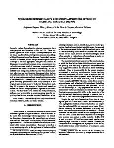


![[PDF]Review Nonlinear Dimensionality Reduction ... - Google Sites](https://m.moam.info/img/260x300/pdfreview-nonlinear-dimensionality-reduction-googl_64771543097c4744708b4b20.jpg)


