Jun 16, 1976 - aspects of double-diffusive convection are the same; only the time and ... I n a double-diffusive situation, using this geometry, Huppert & Manins.
J . F u i d Xech. (19761,VOZ. 78, part 4? pp. 821-854 Printed in Great Britain
82 1
Nonlinear double-diffusive convection By HERBERT E. HUPPERT
AND
D A N I E L R. MOORE
Department of Applied Mathematics and Theoretical Physics, University of Cambridge (Received 16 June 1976)
The two-dimensional motion of a fluid confined between two long horizontal planes, heated and salted from below, is examined. By a combination of perturbation analysis and direct numerical solution of the governing equations, the possible forms of large-amplitude motion are traced out as a function of the four non-dimensional parameters which specify the problem : the thermal Rayleigh number RT,the saline Rayleigh number R,, the Prandtl number u and the ratio of the diffusivities r . A branch of time-dependent asymptotic solutions is found which bifurcates from the linear oscillatory instability point. In general, for fixed u,r and R,, as RT increases three further abrupt transitions in the form of motion are found to take place independent of the initial conditions. At the first transition, a rather simple oscillatory motion changes into a more complicated one with different structure, at the second, the motion becomes aperigdic and, at the third, the only asymptotic solutions are time independent. Disordered motions are thus suppressed by increasing R,. The time-independent solutions exist on a branch which, it is conjectured, bifurcates from the timeindependent linear instability point. They can occur for values of R, less than that at which the third transition point occurs. Hence for some parameter ranges two different solutions exist and a hysteresis effect occurs if solutions obtained by increasing RT and then decreasing RT are followed. The minimum value of RT for which time-independent motion can occur is calculated for fourteen different values of u,r and Rs.This minimum value is generally much less than the critical value of time-independent linear theory and for the larger values of u and R, and the smaller values of r , is less than the critical value of time-dependent linear theory. ~
1. Introduction Since its birth as ‘an ocemographical curiosity’ (Stommel, Arons & Blanchard 1966), double-diffusiveconvection has matured into a subject with a large variety
of applications. Many situations exist in oceanography, astrophysics and chemical engineering, to cite only three areas, where there are two components of different molecular diffusivities which contribute in an opposing sense to the vertioal density gradient. Whether the components are heat and salt, as in the oceanographic situation, heat and helium, as in the astrophysical situation, or two different solutes, as in chemical engineering situations, the qualitative
822
H . E . Huppert and D . R.Moore
aspects of double-diffusive convection are the same; only the time and possibly space scales of the motion are different. I n addition to the many applications, interest in the subject has developed as a result of the marked difference between double-diffusive convection and convection involving only one component, as for example in purely thermal convection. I n contrast to thermal convection, motions can arise even when the density decreases with height, that is, when the basic state is statically stable. This is due to the effects of diffusion, which is a stabilizing influence in thermal convection, but can act in a double-diffusive fluid in such a way as t o release potential energy stored in one of the components, and convert i t into the kinetic energy of the motion. The physical mechanism underlying one of the fundamental forms of doublediffusive motion can be understood from the following parcel argument. Using the terminology of heat and salt, as we shall throughout this paper, consider a fluid whose temperature, salinity and density all decrease monotonically with height. If a fluid parcel is raised it comes into a cooler, less salty and less dense environment. Because the rate of molecular diffusion of heat is larger than that of salt, the thermal field of the parcel tends to equilibrate with its surroundings more rapidly than does the salt field. The parcel is then heavier than its surroundings and sinks. But owing to the finite value of the thermal diffusion coefficient, the temperature field of the parcel lags the displacement field and the parcel returns to its original position heavier than it was a t the outset. It then sinks t o a depth greater than the original rise, whereupon the above process continues, leading to growing oscillations, or overstability as it is sometimes called, which is resisted only by the effects of viscosity. This linear mechanism was first explained by Stern (I96O)j- and explored further in a beautifully written paper (Moore & Spiegel 1966) which develops an analogy between this form of doublediffusive convection and the motion of a flaccid balloon in a thermally stratified fluid. If the temperature gradient is sufficiently:large compared with the salinity gradient, nonlinear disturbances may exist which lead to time-independent motion because the large temperature field is then able to overcome the restoring tendency of the salinity field. An evaluation of the conditions under which this time-independent form of motion can occur is one of the aims of this paper. One of the important aspects of time-independent motion is that the heat and salt transports are very much larger than those in typical time-dependent motions. Thus an evolution calculation for a laboratory experiment, an oceanographical situation or a star will be significantly dependent upon what form of double-diffusive motions exists. The traditional geometry in which convective motions have been quantitatively analysed conhes the fluid between two infinite horizontal planes, heated, and in our case also salted, from below. I n the purely thermal situation, many of the theoretically determined results have been experimentally verified and successfully used to explain various phenomena, as summarized by Spiegel (1971). I n a double-diffusive situation, using this geometry, Huppert & Manins (1973) develop some theoretical results which accurately predict the outcome
t
In a footnote.
Nonlinear double-diflwive convection
823
of a series of experiments in which two deep uniform layers of different solute concentrations were initially separated by a paper-thin horizontal interface. For details the reader is referred to the original paper. The essential comment to be made here is that the theoretical model, which incorporates the seemingly constraining presence of the horizontal planes, was successfullyused in a situation uninfluenced by boundaries. Turning now to an explicit statement of the model analysed in this paper, we consider a fluid which occupies the space between two infinite horizontal planes separated by a distance D . The upper plane is maintained at temperature To and salinity Soand the lower plane at temperature To+ AT and salinity So+ A S . Both planes are assumed to be stress free and perfect conductors of heat and salt. We restrict attention to two-dimensional motion, dependent only upon one horizontal co-ordinate and the vertical co-ordinate, and discuss in 9 7 the consequences of this restriction. We non-dimensionalizeall lengths with respect to D and time with respect to D 2 / ~ Twhere , K~ is the thermal diffusivity, and express the velocity q* in terms of a stream function $ by the temperature T* by and the salinity S* by
q* = (KT/D)
($89
- P,),
T" = T O + A T ( l - z + T ) S*
=So+AS(l-~+S),
so that we can write the governing Boussinesq equations of motion as a-1v2at
- c - ~ J ( + v2$) , = - R, a, T + R, a, s+ ~
a, T+a, $-J($, T) = V 2 T , a, 8 + a, $ - J($, 8)= rV2S,
$ = a;,$
=T =
s=o
4 $ ,
(1.4) (1.5) (1.6)
(2
= 0, I),
(1.7)
where the Jacobian J is defined by J ( f ,9 ) = a,.fa,
9 - a z f a, 9.
(1.8)
We have assumed the linear equation of state where a and are taken to be constant, in the expressions for the body-force term of (1.4). Four non-dimensionalparameters appear in (1.4)-( 1.6): the Prandtl number Q
(1.10)
= V/KT,
where v is the kinematic viscosity; the ratio of the diffusivities (1.11)
7 = KS/KT,
where K~ is the saline diffusivity, which is less than number R, = agATDs/(K, v),
K
~ the ;
thermal Rayleigh (1.12)
824
H . E . Hwppert
and D . R . Moore
where g is gravity; and the saline Rayleigh number
Rs = &AsDs/(KT V).
(1.13)
The fist two parameters characterize the fluid, while the last two characterize externaIIy applied parameters of the model. I n this paper both Rayleigh numbers are positive.? For brevity, we refer to the system (1.4)-(1.7) as 8. Some solutions of 8 were obtained by Veronis (1965, 19686) in terms of truncated Fourier expansions. He concluded from the latter, more accurate, study that, for u 2 1, as RT is increased oscillatory motion first occurs and then at a value of R , greater than Rs the motion becomes steady. Veronis conjectured that, for increasingly large values of Rs,the minimum value of R, for which steady convection can occur tends to R,. The approach adopted in this paper is very different in both numerical detail and interpretation. The numerical methods employed are supported by analytical calculations which allow a larger range of values of CT,7 and R, to be investigated. We find that as RT is increased from zero, steady motion can occur fist, at a value of RT significantly less than Rs. The linear solutions of are discussed in $2. It is shown that the stability boundary occurs at the same horizontal wavelength for both oscillatory and steady linear modes and the possible forms of linear motion are mapped out in an R,, R, plane (figure 1). The horizontal scale of linear theory is then used in the nonlinear investigations discussed in $0 3-7. Results obtained using differenthorizontal scales are similar, as briefly discussed in the footnote on page 828. We focus on the asymptotic solutions of .ul,, that is those solutions which result from long-time integrations of yZ considered as an initial-value problem. We find that these solutions may be oscillatory, aperiodic or steady. Further, there exist ranges of u,7 and RT for which two stable equilibrium solutions of different character exist. These results are obtained from the combined use of modified perturbation theory (as described for example in Sattinger 1973), direct numerical integration of .ul, and the generally known results concerning solutions of nonlinear differential equations. From modified perturbation theory, the analytic form of the equilibrium solutions in the vicinity of the linear modes can be investigated by an ordered expansion about these modes. As the degree of nonlinearity increases, the form of solution is numerically investigated by integrating 8 using finite-difference techniques. The numerical program places constraints on the values of u and 7 for which quantitative results can be obtained. In particular, it is not possible to use the program with u = 7 and 7 = &, the appropriate values for heat and salt in water. However, a sufficient number of different values of u and 7 are investigated to discern the overall pattern of the results. Because it is this If both Rayleigh numbers are negative the analysismodels a fluid in which temperature and salinity increaae monotonically with height. I n this situation the motion is generally
time independent and is due to fluid parcels with downward motion diEusing heat to adjacent rising fluid parcels, much in the manner of a heat exchanger. This form of motion, called salt-hgering, was first explicitly discussed by Stern (1980)and some nonlinear aspects have been considered by Straus (1972).
Nonlinear double-diffwive convwtion
826
overall pattern which is of greatest interest, the discussion of the possible forms of solution is fairly general, with the calculated results being used only as quantitative illustrations.
2. Infinitesimal motions
The results of linearized theory have been derived elsewhere (Stern 1960; Veronis 1966, 19683; Baines & Gill 1969). However, since these results act aa a foundation for the nonlinear aspects of our investigations, we restate them briefly in this section in a manner convenient for future reference. The equations governing infinitesimal motions are obtained by deleting the nonlinear Jacobian terms of (1.4)-( 1.6). The resulting differential system has constant coefficients and a solution in terms of the lowest normal modes
j
+o sin nax +(x, z, t ) T ( x ,z,t ) = Tocos n a x ] socos nax S ( x , 2, t )
(2.1~) e p t sin nz
(2.lb) (2.lc)
leads to the dispersion relationship
+
p9+ (a+7 + 1) k2p2 [(a+7 + OT) k" - n%a2k2(RT - R,)]p + v ~ ~ C S + ~ ~ ~ O ~ C=:~0 (, R( ~ 2 . -2 )~ R T )
where k2 = n2(1+a*). (2.3) Since ( 2 . 2 ) is a cubic with real coefficientsits zeros are either all real or consist of one real root and two complex-conjugate roots. Overstability, which arises when the pair of complex-conjugate roots crosses the imaginary axis, p,, = 0, occurs when a+7
B,(a)
and
=
aflB, + (1 + 7)(1 + T 0 - l ) .E8/(n2U2)
p t = (CTT+ a + 7)k4 - a(RT- R,)n2a2k2.
(2.4)
(2.5)
For fixed values of a and 7 , R,(a) is least for a = 2-4 at which value Pl(n2a2)= yn4,
(2.6a)
(2.63)
and p = kipo, say. Exchange of stabilities, which arises when one of the roots equals zero, i.e. p E 0, or equivalently a, = 0, occurs when
R,(a)
= R&
+P/(n2a2).
(2.7)
As before, R,(a) is least for a = 2-$, at which value we denote R, by
R,
+
= RS/7 ?$+,
(2.8)
where the subscript 6 anticipates the development in subsequent sections. Descriptions of and, where possible, analytic expressions for B,, .,.,R, are given in table 1.
H . E . Huppert and D. R . Moore
826 15 000
-
10000
-
5000
-
+ A
RT
FIQTJR,E 1. The results of linear stability theory for u = 1*0,7 = 0.5. Only the region below the two heavy lines is stable to linear disturbances.Each small pair of axes with its three orosses represents the complex p plane and the relative position of the solutions of (2.2) for the values of RT and Rfi at the origin of the axes.
I n the R,, R , plane the linear stability boundary is a combination of RT = R, and B, = &, as depicted in figure 1 , which presents a complete summary of the linear results for a = 1and 7 = 0.5. For &?, > R,,,, where Rl,s= 9 7 p T 2 ( 1 + a-1) (1 - 7 ) - 1 (2.9) is the value of R, at which R, = &, as RT exceeds R, the conduction state is unstable to an oscillatory mode. This instability occurs because of the physical mechanism discussed in the second paragraph of the introduction. For 0 < RS < Rinm the salt gradient is too small for the mechanism which gives rise to the oscillations to be effective and the conduction state is destabilized by a monotonic mode as RT exceeds R,. For fixed R, > R,,,, as R , increases above R,, the two complex-conjugate roots acquire positive real parts until R , = Rco,say, at which point these roots coalesce on the real axis. The value of Rcocan be determined from the implicit relationship [~+a+a7+-4a ( Rs - Rc o ) - + ( a + 7 + 1)2 +$ $(a+7+1)' 277p
13
1
4
2
= 0,
(2.10)
Nonlinear double-diffusive convection
827
which expresses the condition that (2.2) has a repeated root. The graph of Rco as a function of RB for g = 1.0 and T = 0.5 is presented in figure I. As R, increases above Rco,one of these two real roots increases and the other decreases until at R, = R, the latter root is identically zero. Thus at this exchange-ofstability point, as R, increases, one root of (2.2) decreases through zero, while one of the other roots remains positive, the other negative. For 0 c R8 < R1n6 there is one positive (real) root and two negative roots for all R, > R,. ,Also drawn in figure 1 is the line RT = R,, above which the basic density is statically unstable. I n summary, the conduction solution bifurcates a t R, = R, into a pair of conjugate oscillatory solutions and, at R, = R,, into a monotonic convective solution, where the term monotonic in this paper is synonymous with nonoscillatory. According to linear theory, for 0 < R, < Rl,.,)Bconvection is always monotonic, while for R, > Rln6it is oscillatory for R, < R, < R,, and monotonic for R, 2 Rco.Since R,, > R,, linear monotonic convection is possible only if the basic density is statically unstable. Higher normal modes of the form
W m j
$oshmTax]
T ( x ,z , t ) = Tocos mmax ept sin nmz S ( x ,x , t ) Socos m m x
(2.11a)
(2.llb) (2.11c )
have critical thermal Rayleigh numbers which can be calculated in the same manner as described above. As before, the lowest values occur for a = 2-4. Overstability for the (m,n) mode (using obvious notation) sets in at a thermal Rayleigh number given by (2.12)
and exchange of stabilities a t a thermal Rayleigh number given by
Rg" = R8[T + 2n4m-2(n2+ QmZ))".
(2.13)
The (2,l) modes, with half the horizontal scale of the lowest normal modes, have smaller critical Rayleigh numbers than the (1,2) modes, with half the vertical scale of the lowest normal modes. These higher modes play no essential part in our investigation and are mentioned here mainly for completeness.
3. Finite-amplitude motions The main aim of this paper is to examine how the various instability regions of the previous section extend into the nonlinear domain and in particular to determine the possible asymptotic solutions for given RT and R,. Essentially, this requires the addition to figure 1 of a third dimension representing the amplitude of the motion. For convenience, graphical results are presented by considering planes of constant R,, and asymptotic solutions are hence plotted in an R,, amplitude plane.
H . E . Huppert and D. R . Moore
828
Solutions are obtained by direct numerical integration of .ul,, supplemented by analytical calculations using modified perturbation techniques. The numerical computation is accomplished by approximating .ul, by space- and time-centred second-order difference equations in @, V2+, T and Son a rectangular staggered mesh in the domain 0 < x < a-l= 2 ) and 0 Q z Q 1. The equations incorporate the periodicity conditions = $xz = T, = S, = 0 at 2 = 0 and a-1. From the equations, values of Vz$, T and 8 at the grid points are advanced in time steps of at. The variable $ is then calculated from V2@ by inverting the Laplacian using an implicit finite-difference approximation to Poisson’s equation. This process is repeated for as many time steps as required. The program is an extension of one used originally by Moore, Peckover & Weiss (1973) and is discussed further in the appendix. The appendix also contains a list of almost all the numerical experiments conducted. A full investigation has been carried out for the 14 sets of (Q, T , R,) values displayed in table 3. For each set of parameters, the branch of nonlinear asymptotic solutions emanating from the oscillatory bifurcation point €2, and the branch of monotonic solutions, presumably emanating from the bifurcation point R,, are traced out in an R,, amplitude plane. In particular, the value of R, below which a monotonic solution cannot exist is found (table 3, column 6). The amplitude of any solution could be characterized in a number of different ways, using either local values, such as the velocity or stream function at a particular point, or global values, such as the heat or salt transport, or the kinetic energy. In this paper we find it most convenient to use the horizontally averaged heat and salt transport, or their non-dimensional representation, the thermal and saline Nusselt numbers. These are given by
+
- -
- -
Ns(z) = 1-aES+w8, (3.117 (3.2) where w is the (non-dimensional) vertical velocity and an overbar denotes a horizontal average. At either of the boundaries w = 0 and the second term of (3.I ) and (3.2), which is the direct contribution made to the heat transfer by convection, is zero. In particular, at the lower boundarythe Nusselt numbers are given by A?&(Z)
= l-a,T+wT,
-
-
NT = 1-a5T15=o, Ns = 1-8,8ls=0, (3.31, (3.4) where the value at z = 0 in the representationson the left-hand side is understood. We use either of these two, or where appropriate their maxima, MT and Mg, say, as an indication of the amplitude of the motion. Using a global energy analysis Shir & Joseph (1968) show that for R, 2 0 a suflcient condition for the conduction solution to be the only solution of .sP, is that R, < %$+. However, we find that for all of the parameter space which we investigate, the conduction solution is the only solution for a range of values of R, larger than ?$?-.”. The double-diffusive BBnard problem heated and salted below hence provides an example where straightforward global analysis does not yield attained bounds.? This result should be contrasted with the case of negative
t This conclusion is based on the additional facts that the solutions outlined in this paper for a = 2-4 are relatively insensitive to a change in a to within a factor of 2, and, in particular, that the minimum value of RT for which convection can be sustained at a = 2-4 is only slightly larger than the absolute minimum obtained by varying a.
829
Nonlinear double-diffusive convection
RT and Rsr (heated and salted above), for which Shir and Joseph show that a necessary and sufficient condition for the conduction solution t o be the unique solution of yZ is RT < R,. The next section discusses the nonlinear oscillatory motions and $6 discusses the nonlinear monotonic motions. The relationship between these two equilibrium solutions is discussed in fj6 .
4. The branch of oscillatory solutions
I n the immediate neighbourhood of the oscillatory bifurcation point R,, the nonlinear equilibrium solution can be obtained from a modified perturbation expansion of $. For fixed R,, this is achieved by introducing the new time variable t' = pt (4.1) and expanding each variable as (4.2a-c)
and
RT
=
I; enrn
P
=
C enfin, n=O
03
(4.2d)
n=O m
(4.2e)
where E is a convenient expansion parameter whose value can be determined from ( 4 . 2 d )for given 22,. Substituting (4.1) and (4.2) into 3 and equating like powers of B, we find that (4.34 (4.3b) (4.3c) (4.34 e )
(4.4a) (4.4b) (4.4c) (4.4d,e )
d (k2-[(ifi, + k2)(ijo +7k2)( i r l f i o+ k2)]- in2a2(ro-Rs))fi2-n2a2(ifio +7k2)r2 dfi0
= & 7 n 8 ~ ~[+k2(+P ~{ +&)-"
+
+
(2n% + ifio)-'(7k2 ifio)-'] (ifio k2)R,g
- n-2k2(P +fit)-' + (2n2+ ijo)-'(k2 +ifiO)-l](ifio+7k2)R,},
(4.5)
where in (4.3), (4.4) and in similar equations to be presented below, the real part of each right-hand side represents the variable on the left. Using these results and the definitions (3.2)and (3.3),we h d that as RT +-R, NT 1 + &n"a2(kz+ ijo)-l[tn-z + (2n2+ ij0)-leZit']ril(BT-Rl) (4.6) and Ns 1 + f&X2(7k2 + ij0)-' [&n-"T-'+ (2n27+ifi0)-'eZit']rF1(RT- Bl). (4.7) N
N
H . E . Huppert and D. R. Moore
830
F r u m 2. The solutions rz a n d j z of (4.5) as a function of Rs for (a)u = 1, 7 = lo-*, (b) u = 1, 7 = 0.1, (c) (r = 10, 7 = 0.1 a d (d) u = 7, 7 = &-.
L
1.o
I
I
2.0
I
I
3.0
I
1.0
I
-
I
2.0
I
I
3.0
1
1
I
4.0
F I ~ ~ 3.LThe E oscillatory solution branch for c = 1, 7 = 0.1 and Rs = lo4.---, calculated stable portion of the branch; ---, sketched unstable portion of the branch; --, first approximation to the unstable portion, as obtained from (4.6) and (4.7).
Graphs of r2 and b2as functions of R, for four values of CT and 7 are displayed in figure 2 and the maximum value of N,, obtained from the right-hand side of (4.7), is displayed in figures 3 and 5 for different values of CT,7 and R,. For small R,, r2 is positive. Thus R, increases with amplitude (2M,or M,) and the bifurcation point is supercritical. It can be shown in general (see for example Sattinger 1973) that, since they arise from a supercriticalbifurcation, solutions on this branch will be stable with respect to any further linear two-
Nonlinear double-diffusive convection
831
dimensional disturbance. The essence of this result can be explained by consideration of the associated potential energy function, for which all extrema represent equilibrium points, with potential energy minima (maxima) corresponding to stable (unstable) asymptotic solutions. For RT larger than the value at a supercritical bifurcation point, the asymptotic solution of zero amplitude is unstable and hence is a t a potential energy maximum. With increasing amplitude, the next equilibrium point is at a potential energy minimum and hence corresponds to a stable asymptotic solution. The numerical solution of $ for small R, confirmed this stability and the comparison between (4.6) and (4.7) and the numerical results is seen from figure 5 to be very good for quite a range of RT - R,. For large R,, r2 is negative and the bifurcation is thus subcritical. Solutions on subcritical branches are unstable because the zero-amplitude solution, being stable, is at a potential energy minimum and hence the next equilibrium point is at a potential energy maximum. Unstable solutions cannot be obtained from the scheme we have employed for the numerical solution of S$. However, it can be inferred from previous studies that the branch continues, and solutions on it are unstable, until a minimum value of R,. is reached. The branch then continues with the amplitude of the motion increasing with increasing RT. The asymptotic solutions on this portion of the branch correspond to potential energy minima and the associated solutions are hence stable (and time dependent). An example of this behaviour is depicted in figure 3. Comparisons of the period of the nonlinear motions obtained from (4.2e),(4.3e) and (4.5)and from the numerical solution of g are made in figure 4 for u = 1.0, r = 10-4 and for three values of R,. These three comparisons reflect the general tendency that for small values of R,, carrying out the perturbation procedure to the order indicated (determining only Po, and p2)leads to results in good agreement with the exact solutions, while for larger values of R, further terms are needed in order to obtain useful information. For values of RT beyond the range of applicability of the perturbation procedure, the numerical solution of is needed to investigate the oscillatory branch further. A summary of the results of such an investigation is shown in figure 5 and table 3. The branch continues in the RT, amplitude plane with the amplitude increasing with increasing R,. Along this branch the period of the oscillation increases monotonically because of the increasing influence of the temperature field. Expressed in terms of the motion of a typical fluid particle, the explanation is that during its oscillatory displacement the particle experiences a restoring force which decreases as R, increases, and hence the period increases. Figure 6 presents for one value of cr, r , RT and R, a typical plot of NT and N, against time. The phase delay of N, with respect to NT is clearly seen. This delay occurs because the salt field diffuses more slowly than the temperature field. The slower diffusion of salt is also the reason why both the mean and the range of are larger than those of NT.Expressing Ns as a Fourier series and thus evaluating the power a t each frequency, we obtain the result shown in figure 7 (a). This figure, which is to be viewed as an indication of the degree of nonlinearity of the motion, displays the large amount of power in the fundamental and the smaller, but by no means insignificant, power in the higher harmonics.
832
H . E . Huppert MlcE D . R. Moore
I
I
I
0.7
I
I
I
0.8
I
I
0.35
0.9
I
0.40
2.h
1
1
0.45
21.P
I
I
0.19
I
0.20
I
I
0.21
I
2.lP
FIUURE 4. The period of oscillation 2n/p as a function of RT for (r = 1, 7 = 10-1 and (a) RS = lo8 (R,= 1797), (b) Rs = 10% (R,= 3220) and (c) Rs = lo4 (R,= 7720). -, result obtained from the numerical calculation of 9,;--, result obtained from the modifkd perturbationexpansion of 8 4.
Diagrams of the stream function, temperature, salinity and resulting density fields for one value of cry7 and Rsare shown in figure 8. Eight representations of the fields, equally spaced in time and commencing when the maximum point of N , is achieved, are presented which cover a complete cycle of NT and N,. The eight times are indicated in figure 6. The period of the basic fields is twice that of N, and Ns and thus the figure presents these fields over only half a period. Their continuation occurs in the following manner: the ninth representation of the stream function field is the negative of the f i s t in the depicted series, the tenth is the negative of the second and so on; and the ninth representations of the temperature, salinity and density fields are the reflexions about a vertical edge of the first representations, and so on. Examining the stream function field first, we see that fluid particles move back and forth in their predominantly circular motion around part of the cell. The intensity of the motion reaches a maximum before the maximum of either N, or ATs, which as explained above is the essential characteristic of oscillatory doublediffusive motion. At one point in this oscillation, rising hot fluid and sinking cold fluid produce the reflected S-shaped contours of the first representation
Nonlinear double-diffmiveconvection
3.0
2.0
833
4.0
MS
I
I
I
2.0
3.0
4.0
i
5.0
MS
FIQURES B(a,b). For caption see page 834.
53
FLY
78
2.. /I’
H . E . Huppert and D.R.Moore
a34
....................... ...(..
(4
1 iooa
Monotonic
1oooo
RT 9000
8000
I
I
I
2-0
1
6.0
4.0 MS
400C
.....4........
3500
RT 3000
I
2.0
I
I
I
I
4.0
6.0
I
I
8.0
I
I
10.0
MS
F ~ a m 5. The stable solution branches in an RT, MS plane for (a)u = I, 7 = lo-&,Rs = 108, (b)u = 1 , 7 = 10-1,Rs = lo*, (c) = 1 , =~ 10-1, Rs = IO4md (d)u = 1 , =~0.1, Ra = 10%. For R, < RT < R, both local maxima are shown and for R, < RT < R, the rapidly oscil-
lating curve indicates that no definite maximum can be assigned to the aperiodic motion in this range. The dots indicate the transitions that can take place between the oscillatory and monotonic branches. T h e dashed curve is the first approximation to the oscillatory solution branch, aa obtained from (4.7).
Nonlinear double-diffusive convection
1
1
1
1
1
1
1
1
I
835
-
0
0.025
0.05
t
FIGURE 6. The thermal and saline Nusselt numbers rn a function of time for R, < RT = 8600 < R,, Rs = lo4, u = 1 and 7 = 10-*. The marks on the time axis indicate the times a t which the stream function, temperature, salinity and density fields are displayed in figure 8. The horizontal line in the bottom right-hand corner represents 0.05 non-dimensional time units.
10.0
-
1.0
-
0.1
--
0.01
-
-
0~0010
0
FIGURE 7. The spectral lines of &(t) for u = 1,7= lo-&,RS = lo* with (a)R, < RT = 8600 < R,and (b) R, < RT = 9800 < R,.
of the temperature field. As the oscillation proceeds, the fluid reverses its direction and the temperature field relaxes, until in the fifth representation the horizontal temperature gradients are extremely small. In the last few representations, the horizontal temperature gradients increase until the temperature contours reach their maximum S-shape again. The salinity field is similar to the temperature field except for the following important differences. First, the salinity field attains its maximum structure after the temperature field, for the reason explained previously. Second, owing to the relatively slower diffusion of salt, the horizontal salinity gradients, which decrease to a large extent by diffusion, do so less rapidly than the horizontal temperature gradients. However, they increase approximately as rapidly because the increase occurs by the different process of advection, as evidenced by the increasing stream function field. Turning now to the density field, we clearly see the relative oscillatiow of the 53-2
H . E . Huppert and D. R.Moore
836
(4
UJ)
tc)
(4
(el
FIGVRE 8. "he basic fields for R p = 8600, Rs = lo4, u = 1 and 7 = 10-4. (a) "he stream function $ with a contour spacing of 0.0115. (b) Perspective representations of (a)viewed from a point 8 cell widths from the centre of the cell at an elevation of 0.3 red from the horizontal plane and an azimuthal angle of 1.0 rad measured clockwise. (c) Thenondimensional temperature T*/AT with a contour spacing of 0.2. (d) The non-dimensional salinity S*IAS with a contour spacing of 0.2. (e) The non-dimensional densityp*/Ap, where Ap is the density excess a t the bottom of the cell over that at the top, with a contour spacing of 0.3.The H and L on the density representations indicate the regions of relatively heavy and light fluid.
heavy and light regions of the fluid. The comparison of the density field with the stream function field indicates the continual exchange that takes place between the potential energy and kinetic energy of the system. At one extreme, in the second representation, the stored potential energy is close to its maximum, with large regions of heavy fluid lying above relatively lighter fluid, and the kinetic energy is almost zero. Thereafter, the kinetic energy increases at the expense ofthe potential energy until at the other extreme, in the seventh representation,
Nonlinear double-diflwive convection
837
The lowest-mode linear instability point for oscillatory motion (overstability) The transition point between motion with one maximum per period and that with two maxima per period The transition point between motion with two maxima per period and aperiodic motion The transition point between aperiodic motion and time-independent motion The maximum value of RT for timedependent motion The minimum value of RT for timeindependent motion The lowest-modelinear instability point for time-independent motion (exchange of stabilities) The coalescencepoint of the two (complexconjugate) eigenvalues of linear stability theory The (m,n)-mode linear instability point for oscillatory motion
RT = R,
RT = Roo[equation (2.10)]
The (m,n)-mode linear instability point for time-independent motion The value of Rs at which RT = R, intersects RT = R, The value of Rs above (below)which the lowest exchange of stability point is a subcritical (supercritical)bifurcation TABLE1 . Nomenclature
4.0
1.0
-
l--+--+
0
0.05
0.1
t FIGURE 9. The thermal and saline Nusselt numbers as a function of time for R, < RT = 9800 < R,, Rs = lo4, u = 1 and 7 = 10-4. The marks on the time axis indicate the times a t which the stream function, temperature, salinity and density fields are displayed in figure 10. The horizontal line in the bottom righthand corner represents 0.1 non-dimensionaltime units.
H . E . Huppert and D. R.Moore
838 u = 1.0,
RT 7720(=R1) 7750 7800 8200 8600 9000 9200 9400 9600
7
= lo-&, R~ = 104
{z {z
{$
9800 10200-1100
Period 0.0940 0.0949 0.0954 0.102 0.111 0.120 0.125 0-123 0,134 0.126 0.132 0.122 0.144 0.126 0.140 0.122 0.155 0.126 0.151 Aperiodic
u = 1.0, RT 2535(=R,)
7
= 0.1, R s = 10t
2600 2660 2720 2780 3000 3250 3325 3400
: :{
3500 3600-4 100
{z
Period 0.145 0.146 0.150 0.154 0.159 0.183 0.205 0.212 0.192 0.236 0.209 0.222 0.189 0.256 0.206 0.239 Aperiodic
TABLE2. The period of NT and Ns. For R, < RT < R, the time between the smaller maximum and the following larger maximum is given first followed by the time between the smaller maximum and the preceding larger maximum for NT.The next line consists of these times for Ns.
FIQURE 10. For caption end remainder of figure see opposite page.
Nonlinear double-diffwive convection
839
FIGURE 10. The basic fields as in figure 8 for RT = 9800, RS = 104, cr = 1, r = 10-*.The contour spwing in the stream function representations is 0.0115, in the temperature and salinity representations 0.2 and in the density representations 3-0.
the stored potential energy is close to its minimum, with the density increasing with height everywhere, while the kinetic energy is close to its maximum. As R, increases, this form of motion continues until R, reaches a specific value, B,, say. At R, = R, the motion changes in form. Either the motion becomes time independent, a situation discussed at the end of this section and in greater detail in the next section, or, the more general case, the motion develops a further structure as is indicated in the form of N, or N, as a function of time, as graphed in figure 9. I n both N, and N, there are four extrema, two maxima and two minima, per period, where the period is defined in the usual sense as the time between two identical states. As seen in figure 9 and table 2 the time between the smaller maximum and the preceding larger maximum is greater than the
840
H . E . Huppert and D. R. Moore
time between the smaller maximum and the following larger maximum. This holds for both NT and N,. As RT increases above R, these times evolve continuously from the single period exhibited by NT or N, for RT just below R,. The power at each frequency of the Fourier representation of N, is shown in figure 7 (b),from which it can be seen that this second form of motion has much more structure than the first form discussed previously. The physical reason for this form of motion is that the increasing temperature difference attempts to induce monotonic motion. Fluid near one of the lower corners of the cell rises, sinks by a different route, rises by a smaller amount in an attempt to readjust the form of motion, sinks again and the total form of motion is then repeated. Other fluid particles in the cell move accordingly, as is shown in figure 10. This figure presents the stream function, temperature, salinity and density fields at sixteen equally spaced times over a complete cycle of NT and N,. The figure is constructed in a manner similar to figure 8 except that a complete cycle of NT and N, is now equal to a complete cycle in the motion fields rather than the previous half-cycle. The first representation is, as before, at the maximum of N, and the times of each representation are indicated in figure 9. The asymmetry of the two half-cyclesis evident in all the fields, in contrast to the situation when RT < R,. Closely following the stream function field of maximumintensity (representation 16),the third, fourth and fifth representations of the stream function field show how part of the fluid moves with a predominantly vertical component through the interior portion of the cell. This motion is reflected in the corresponding density field, where heavy fluid descends just to the left of the middle of the cell and light fluid rises just to the right. The flow results in a temperature structure with an interior maximum and minimum (representations 4, 5 and 6) and a similar salinity field somewhat delayed (representations 5, 6 and 7). The first part of the cycle is thus very different from that with RT < R,, though the second part is quite similar, and almost all of the discussion of figure 8 applies to it. In terms of modern mathematical jargon, the solution for R, less than R2is on a sphere, while for RT greater than R, it is on a torus, and the transition at RT = R, is called a bifurcating torus (Hirsch & Smale 1974). This form of motion occurs until RT = R,, say, at which value a transition either to a time-independent solution or, more generally, to a disordered, aperiodic form of motion occurs. No stable asymptotic motion with three, four or more maxima per cycle was found, though it may be that such motion exists in a different parameter range from the one examined. It is difficult to describe the aperiodic form of motion further. Figure 11 presents for one value of r,7 , RT and R, a plot of N, and N, against time. Long computational runs have not revealed any periodic structure. It may be that the solutions are in some way similar to the apparently aperiodic solutions of a class of ordinary difference equations found by May (1976) to be made up of a finite number of periods. But, as discussed by May, the motion is so complicated that assigning a period to it is of very little use in understanding the motion or interpreting the results. Aperiodic motion continues to exist for increaaing R, until for RT = R4, say,
841
Nonlinear double-diffwive convection
3.0
1.o
5.0
3.0
1.o
0
0.25
0.5
t FIGURE 11. The thermal and salineNusselt numbers aa a function of time for Q = 1,7 = 10-* and (a)R, < RT = 8600 < R,,(a) R, < RT = 9800 < R, and (c) R, < RT = 11000 < R,. The horizontal line in the bottom right-hand corner of (c) represents 0.5 non-dimensiond time units for each of the three graphs.
an asymptotic time-dependent solution can no longer be maintained and the only asymptotic solutions are time independent, a form of motion which will be analysed in the next section. For some values of a, T and B, this timeindependent form occurs before the solution passes through the two-maximaper-cycle form of motion or the aperiodic form. Transitions which do occur are indicated in table 3. It is seen that for small values of R, only the simplest form of time-dependent motion occurs, and that for large values of R, the timedependent branch includes the three different types of motion. Also tabulated in table 3 are the linear oscillatory and monotonic critical Rayleigh numbers P 1 1 and Ril for the second lowest mode. These Rayleigh numbers do not seem connected in any way with the Rayleigh numbers R,, R, or R4. For future use we denote by Bi the value of RT at which the transition to an equilibrium time-independent solution occurs.
5. The branch of monotonic solutions For all R, > 3;monotonic motion ensues. As indicated in figure 12, such a
form of motion exists in a double-diffusive fluid because the temperature field can produce an almost isosaline core, with all salinity gradients confined to boundary layers, which are thinner than the thermal boundary layers by an amount 7-4. I n these salinity boundary layers, the effect of the stabilizing salinity gradient on the temperature field is small because of the different diffusivities. For sufficiently high RT the destabilizing temperature effects can
1346 2535 6296 9046
1649 3634 9912 14503
103 10f 104 1.5 x 10⁴
103
1750-1775 3325-3400
4200-4300 9200-9400
-
R,
U=
10.0,
d = 1.0, 1775-1800 3500-3600
7
R,,, = 8.0 2100-2200 1700-1800 46004800 3700-3800 9700-10000 9300-9600 13400-13700
7 = 0.1,
= 0-1, R,,, = 14.6 1900-2000 1700-1800 4100-4200 3500-3600 < 10200 8800-9000 12300-12700
R4 R5 d = 1.0, 7 = lo-*, R,,, = 192.3 2275-2300 2000-2050 44004500 4100-4150 9800-10200 11000-11200 10400-10500 < 15000 15600-15800 15000-15200 19400-19600 24200-24400 R3
10658 32280 100658 150658
10658 32280 100658 150658
3820 10658 32280 48092 63903 79714
R,
2379 4365 10643 15233
2141 3330 7091 9841
2936 4359 8859 12150 15440 18731
R;1
104 1.5 x 10⁴
A blank indicates that the value at which that specific transition takes place was not calculated.
TABLE3. The various transition points. A dash indicates that for that particular value of u, 7 and Rs no such transition occurs.
1797 3220 7720 11010 14301 17592
103 10% 104 1.5 x 10⁴ 2.0 x 10⁴ 2.5 x 10⁴
10%
Rl
RS
~
11315 32938 101315 151316
11315 32938 101315 151315
4477 11315 32938 48749 64561 80372
R",'
Q
2
5
9
b
&
$
%
8
kj
Nonlinear double-diffusive convection
843
(f1 fs) (h) FIGURE 12. The basic fields for RT = 10700, RS = lo4, u = 1 and T = 10-*. (a)The perspective representation of the stream function viewed from the same point P as in figure 8. (b) The perspective representation of the vorticity Vz$ viewed from P . (c), ( d ) , (e) The non-dimensional temperature, salinity and density with contour spacings of 0.2, 0.2 and 1-0 respectively. (f)The mean temperature profile averaged across the cell. (9)The mean salinity profile. ( h )The mean density profile. thus overcome the restoring effects of the salinity. This steady form of motion is a very efficient way of transporting heat and salt and thus the equilibrium Nusselt numbers undergo a discontinuous increase as the solution changes from the oscillatory branch to the monotonic branch. The fields displayed in figure 12 are typical of solutions on the monotonic branch. These all consist of steady, roughly circular motion with the largest vorticity in the central region of the cell. There is rising hot salty fluid adjacent to one edge of the cell and sinking relatively colder, fresher fluid adjacent to the other edge. The mean temperature and salinity gradients illustrate the thin, principally conductive, boundary layers and the larger, principally convective, interior, in which the mean gradients are very much smaller. The mean density gradient has a double structure in the boundary layer, due to the opposing influences of the temperature and salinity, and a much more uniform distribution in the interior. As RT increases above Ri the Nusselt numbers also increase. For very large RT and fixed R,, the temperature field and thermal Nusselt number are very similar to those for the purely thermal problem (Rs= 0) a t the same RT. Using the mean-field equations, Huppert (1972) suggests that at infinite Prandtl number NT = 0.224 [ I - (d&?,g/RT)]+R& (5.1) and i& = 7-4 NT (5.2) as R T + m . For a Prandtl number of 1-0, the multiplicative constant in (5.1) is increased, so that NT = 0.238[1.-(74R,/RT)]~R~ (C = 1 , RT-tm).
(5.1')
Nusselt numbers obtained from the numerical solution of Ytfor o = 1 are compared with those calculated from (5.1') and (6.2)in figure 13. It is seen that the agreement is rather good.
H . E . Huppert and D. R. Moore
a44 10.0
-
8.0
-
6.0 4.0
-
2.0 -
t
0
10 000
5000
15 000
RT
FIGTJRE 13. The thermal and saline Nusselt numbers ae a function of RT for cr = 1, 7 = 10-* and Rs = los. The crosses are the results obtained from the numerical solution ofYt and the curves are the results (5.1’) and (5.2) obtained from the mean-fieldcalculations.
The accurate investigation by Moore & Weiss (1973) of the purely thermal problem indicates that an @ relationship between NT and R, holds for 5 < R/R,
Ri. As R, is decreased below R;, an equilibrium monotonic solution continues to exist, with decreasing Nusselt numbers, until R, = R,,say. Further decrease in R , leads to a solution on the oscillatory branch already described, or, if R, < R,,to conduction. There is thus a hysteresis between these two different modes of motion, which will be discussed further in the next section. It is entirely reasonable to suppose (but has not been rigorously proved) that the nonlinear steady branch emanates from the bifurcation point at R, = Re. The behaviour of the solution about RT = 22, can be obtained by using modified
Nonlinear double-diffusive convection
845
perturbation theory in the same way as discussed in $ 3 except that all time derivatives are neglected. We find that: T and S are the same m ( 4 . 3 ~ ) if Po is set equal to zero and eif is set equal to 1 therein; r,, = R,,; T,and 8, are the same as ( 4 . 4 ~ (withbe ) set equal to 0 and eit' to 1); and
+,
r, = @r2(R6 - 7-3 R,) a%-2.
Using these results and the definitions (3.3), (3.4) and (4.2), we find that and
NT
N
I
+ 2(R6-7-'RS)-l (RT -Re)
(RT +-Re)
(5.3) (5.4)
N, N 1+27-2(R,,-7-3R,)-1(RT-R,,) (R,+-R6), (5.5) independent of a. The monotonic branch hence emanates from a subcritical bifurcation point (r2 c 0 ) if
R6 = 7-lRS + %c+ < 7-3R8
(5.6a, b)
and from a supercritical bifurcation point otherwise. Rearranging (6.6b), we find that the bifurcation point is supercritical for 0 < R, < Rbi, say, and subcritical for R, > Rbl,where
Rbl = Yh2(7-l -7 ) - l .
(5.7)
By comparison of (5.7)with (2.9)it is apparent that Rbi
< Rln6.
(5.8)
Hence, for that range of R, for which linear theory predicts the onset of an oscillatory instability, the accompanying linear monotonic mode bifurcates subcritically. Solutions on this subcritical branch are unstable to time-dependent twodimensional disturbances until R , attains a minimum value. The branch then continues, and solutions on it are stable, with the amplitude of the motion increasing as R , increases. We identify this part of the branch as the one discussed at the beginning of the present section and displayed for four values of cr, 7 and R, in figure 5 . We have not rigorously proved this identification but no other possibility seems at all plausible. A parabola of the form
R , = a ( % - N ~,m in )~+R , (5.9) has been fitted through the three calculated cases on the monotonic branch with the lowest values of R , (seetable 6 ) .The values of the saline Nusselt number at the minimum point, N,, min, are tabulated in table 4 for as many values of 6, 7 and R, for which it was believed that the curve fitting could be accurately carried out. The results of a similar procedure using the numerically obtained values of N, are also tabulated in table 4. The two procedures lead to values of R, which differ by at most l % , a satisfactory amount considering that the procedure involves extrapolation. The unstable portion of the monotonic branch of solutions might be approximated by (5.10) RT = ( R 6 - R 6 ) ( N 8 , m l n - N S ) 2 (NS,min-1)-2+R5,
H . E . Huppert and D . R.Moore
046
Rs
NT,IUln
NS,mln
U=
1.0,
1.64 2.05 2.75 3.13
103
104 104 1.5 x 104
= lo-*
3.07 3-67 4.71 5-43 U=
1.64 2.26
103 109
7
RdT)
RdS)
2000 4110 10450 15060
2000 4110 10430 15050
1740 3570
1760 3570
1.0, 7 = 0.1 5-51 6.94
TABLE4. The minimum values of R T and the corresponding thermal and saline Nusselt numbers for which monotonic convection can occur. These results are obtained by extrapolation of the three calculated solutions on the monotonic branch with the lowest value of RT. U=
Rs 103
105 104 1.5 x 1.04
1.0,
7
-dRT/dNs 1.4 4.4 14 21
=
- (dRT/dNs),, 1.7 4.9 12 15
d
Rs 10s
= 1.0,
- dRT/dNs
10%
4.9 16
7
= 0.1
- (dRT/dNs)psr 3.9 9.7
TABLE5. The gradient in the RT, Ns plane (of the unstable portion) of the monotonic branch at R T = R,. dRTldNs is the gradient obtained by modified perturbation theory and (dRT/dNs), is that obtained from fitting a parabola through the minimum values of table 4 and the point R T = R,, NS = 1.
a parabola which has a minimum of RT = R, a t Ns = N,, and passes through the point RT = R6,N, = 1. The slope of this parabola at NB = 1, (dRT/dNs)par say, is given by (dRT/dN,)par = - 2(R6 - R5)RB, min - 1Y. (5.11) This is compared in table 5 with the value
dRTfdNs = 47’(& - T ~ R ~ ) ,
(5.12)
which is the correct slope of the steady branch at Ns = 1 as analytically determined by (5.5). Considering the simplicity of the parabolic representation (5.10) and the large differences between R, and R6, we find the agreement between the two results to be quite good and conclude that (5.10) is a fair representation of the unstable portion of the monotonic branch.
6. The relationship between the branches of oscillatory and monotonic motion As is clearly evident from figure 5 and table 2, the oscillatory and monotonic branches take quite different relative positions depending upon the values of cr, 7 and R,. The influence of these parameters can be summarized as follows. The linear steady mode is independent of u because fluid particles undergoing steady linear motion conserve their momentum. Along the nonlinear part of the steady
Nonlinear double-di&.sive convection
847
branch the motion is only weakly dependent upon cr for the values of Q we are considering (a2 1), just as in purely thermal convection (cf. Veronis 1966; Moore & Weiss 1973). By contrast, the motion on the oscillatory branch is quite dependent upon the value of cr because the magnitude of the phase lag between the temperature and displacement field, which drives the motion, is determined by cr. By way of contrast, the whole steady branch is strongly dependent on the magnitude of T because its value indicates how slowly the salt field diffuses, and hence how effectively the salt field can overcome the tendency of the temperature field to drive steady convection. Along the oscillatory branch, on the other hand, the value of 7 determines the phase lag between the salinity and temperature field, a lag which has only a small influence on the motion. The value of R,, which indicates the magnitude of the stabilizing salt field, has a large influence on both branches. Table 3 and the discussion in the last two sections summarize the various different orientations of the two branches and the hysteresis loop that connects them. Of particular interest is the value of R,,the least thermal Rayleigh number for which (nonlinear) monotonic convection is possible. Table 3 presents upper and lower bounds to R,for various values of a,7 and R,. These are drawn on figure 14. Consider first figure 14 (a),which presents the bounds to R5for cr = 1,7 = 10-4, and six values of R,. For the four lowest values of R,, R,lies below R,,and above both R, and R,.For the two highest values of R,, R,lies below R,, but above R,. An interesting observation, to be exploited further below, is that for all but the lowest value of R, the four ranges within which R, lies can be joined by the straight line R, = 1200+0-92R, (6.1) and this straight line only just passes beyond the range of R, when R, = 103; (6.1)suggests R, = 2120 while the calculated range is 2000-2050. Decreasing 7 to 10-l without altering Q, we obtain the results plotted in figure l 4 ( b ) .The five ranges for R, are, as expected, all less than those for 7 = 10-1. For R, = lo4 and R, = 1.5 x lo4,R, is less than R,. The straight line
R,
= 1043+0*777R,
(6.2)
passes through the ranges calculated for R, for the three larger values of R, but lies slightly above that calculated for R, = lo3; (6.2)suggests R, = 1820 while the calculated range is 1700-1800. No calculated value of R5is less than the linear oscillatory value R,,and extrapolation of (6.2)beyond R, = 1.5 x lo4,an admittedly dangerous procedure, suggests that, for these values of cr and 7, there is no value of R, for which R, < R,. However, an appreciation of the different dependences of the position of the oscillatory branch and the steady branch on a suggests that by increasing cr it may be possible t o decrease R, below R,. The ranges of R, for cr = 10 and 7 = 10-l are plotted in figure 14(c). For R, = 104 or 1.5 x lo4, R, is less than both R, and Rs.Thus for these values of cr, 7 and R,, (nonlinear) monotonic convection can occur when the fluid is
H.E . Hwppert
848
and
D. R. Moore
/
I
/
20 ooc
RT
/ R ~ = R ~ 10000
I
0
0
I
10 000
5000
I
I
20 000
10 000
15 000
Rs FIGURES 14(a, 6 ) . For caption see opposite page.
J
Nonlinear duuble-cliffuaive convection
849
15000
I 10 000
RT 5000
/
I
5000
0
I
1
10 000
15 000
Rs
F ~ a m 14. The minimum value of B r for which monotonic convection can oocurfor (a)u = 1, 7 = 10-4, (b) u = I, 7 = 0.1 and (c) (r = 10,7 = 0.1. The vertiod bars represent the regions within which the minimum OCCUI‘EI. The long-dashed straight lines (--) in (a),(a) and (c) are (6.1),(6.2) and (6.3) respectively.
statically stable and linear theory predicts the existence of only a conduction solution. As before, there is a straight line,
RT
(6.3)
= 1033+0*844R,g,
which passes through the ranges of R, for the three larger values of Rs but lies slightly above that calculated for R, = lo3; (6.3) suggests R, = 1877, while the calculated range is 1700-1800.
7. Discussion and conclusions Three-dimensional effects in the problem studied should be minimal for the following reason. I n purely thermal convection between rigid boundaries, theoretical analysis indicates that two-dimensional rolls are stable to threedimensional disturbances within a closed region of the R,, a plane commonly referred to as the ‘Busse balloon’ (Busse 1967). Quite extensive experimental investigation has confirmed the existence and shape of the balloon (Busse & Whitehead 1971), and in particular the maximum value of RT = 22600 for which very large Prandtl number two-dimensional rolls are stable. In contrast, theoretical analysis of purely thermal convection between free boundaries indicates that the balloon is still ‘open’for infinite Prandtl number at RT = 20 000 (Straw 1972); that is, infinite Prandtl number two-dimensional rolls between free boundaries are stable up to at least RT = 20000. It is commonly believed, and correctly in our opinion though no proof is yet available, that the Busse balloon for free boundaries remains open as RT tends to infinity. Arguing by 54
FLY
78
850
H . E . Huppert and D. R. Moore
analogy, we conjecture that the double-diffusive convective rolls between free boundaries treated herein are also stable to three-dimensional disturbances for all RT. The major conclusions of the work presented in this paper are as follows. Nonlinear asymptotic solutions of Ytbelong to one of two branches. One is an oscillatory branch, which emanates from the linear oscillatory mode, either supercritically or, for sufficiently large values of R,, subcritically. In general, as RT is increased, the solution along this branch alters in such a way that the associated Nusselt numbers change from one maximum per period (figure 6), to two maxima per period (figure 9) to being aperiodic (figure 11). For sufficiently small R, this branch does not exist at all. The other branch is composed of steady solutions, which emanate from the linear monotonic mode. Unless R, is extremely small this bifurcation is subcritical. I n this general (subcritical)case, solutions on the monotonic branch are unstable until the branch passes through its minimum value of RT, whereafter the solutions are stable - at least in two dimensions. Stable solutions on both branches can exist at the same values of RT, R,, Q and T . This leads to a hysteresis effect if solutions obtained from increasing and then decreasing RT are followed. Depending upon the value of Q, T and R,, as RT increases, instability may first occur as an oscillatory mode, either linear or nonlinear, or as a steady mode, either linear if R, is very small or nonlinear otherwise. Thus nonlinear time-dependent double-diffusive convection can occur when linear stability theory indicates the existence of only a conduction solution, in contrast to the conjecture by Veronis (1968b). Finally, existence of an aperiodic solution which at a critical value of RT becomes steady, by changing from one branch to another, indicates that by increasing RT disordered motion can be suppressed. While these conclusions hold exactly only for double-diffusive convection heated and salted from below, they act as a guide for a number of other problems. Amongst these are: convection in the presence of a magnetic field, currently being studied by N. 0. Weiss (see Prigogine & Rice 1975, p. 101); convection in a rotating system, a preliminary study of which has been undertaken by Veronis (1968a); and convection accompanied by a strong Soret effect, whereby concentration gradients are induced by thermal gradients, as discussed in a number of papers in Prigogine & Rice (1975). The conclusions are not appropriate for double-diffusive convection heated and salted from above (salt-fingering), for which all asymptotic solutions are time independent.
It is a pleasure to acknowledge the help given to us by Dr Joyce Wheeler with the computations and graphical output of this paper. We also benefited from stimulating discussions with S. H. Davis, D. 0. Gough, L.N. Howard, N. Koppell, W. V. R. Malkus, J. Pedlosky, E. A. Spiegel, G . Veronis and N. 0. Weiss. The research was supported by grants from the Science Research Council and the British Admiralty.
851
Nonlinear double-diffwive convection
Appendix. Numerical considerations The numerical solutions of .sP, were obtained by the methods described briefly in $ 3 and in detail by Moore et al. (1973), in which paper the parameters K , K
R' and v are related to the parameters used in this paper by K
=
(gRT)-*,
~ , g =
T(~R,)-*, R' = Rs/RT, v
= g/RT.
~ ,
(A 1a-d)
The majority of the calculations were performed by covering the region O