Nonlinear Dynamic Positioning of Ships with Gain-Scheduled Wave Filtering Guttorm Torsetnes2 , Jérôme Jouffroy1 and Thor I. Fossen1,2 1 Centre
for Ships and Ocean Structures Norwegian University of Science and Technology NO-7491 Trondheim, Norway
2 Department
of Engineering Cybernetics Norwegian University of Science and Technology NO-7491 Trondheim, Norway
Email:
[email protected],
[email protected],
[email protected] IEEE Conference on Decision and Control (CDC’04), Paradise Island, Bahamas, 2004 Abstract— This paper presents a globally contracting controller for regulation and dynamic positioning of ships, using only position measurements. For this purpose a globally contracting observer which reconstructs the unmeasured states is constructed. The observer produces accurate estimates of position, slowly varying environmental disturbances (bias terms) and velocity. The estimates are automatically adjusted to the present sea state by gain-scheduling the wave model parameters in the observer. Finally, the estimates are used in a nonlinear PID control law and the stability proof of the observer-controller is based on a separation principle for contracting systems in cascade.
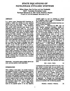
I. I NTRODUCTION One of the most important issues to take into account when designing dynamic positioning (DP) systems for marine vessels, is wave filtering (Balchen et al. [1], Fossen [3], [4]). The total vessel motion is modelled as the superposition of low-frequency (LF) vessel motion and wavefrequency (WF) motions, and an observer is needed to reconstruct the LF motions from the position and heading measurements (sum of the LF and WF motions), see Fig. 1. In Grøvlen and Fossen [9], uniform global exponential stability (UGES) of a DP system (ship model, observer and control law) was proven by using observer backstepping. An extension of this paper to vectorial backstepping is found in Fossen and Grøvlen [5]. These papers can be regarded as the first attempt to design a fully nonlinear DP-control system, since wave filtering and bias estimation were not included. In Fossen and Strand [6] an UGES observer with wave filtering capabilities and bias estimation was designed using passivity. An extension of this observer with adaptive wave filtering appeared in Strand and Fossen [18] while a more detailed description of passive wave filtering in DP is found in Strand [17]. In Loria et al. [15] the same observer was used with a PD-type control law, and by using the separation principle of Panteley and Loria [16], it was shown that the DP system was uniform global asymptotic stability (UGAS). More recently, in Lindegaard [12], this result has been extended to the case where acceleration measurements are available. It is also shown
that the resulting observer-controller system, nonlinear PID controller with acceleration feedback and UGES observer, is UGAS by using the separation principle of Panteley and Loria [16]. Except [18], all these designs assume that the WF model parameters does not change during operation, and that the WF model parameters are known a priori, which is not a realistic assumption. The sea state is constantly changing, and therefore the observer should be able to automatically adjust the reconstruction of the LF motion in accordance with the varying sea state. In this paper, it will be shown that this can be done by gain-scheduling the WF model parameters from on-line measurements. This is referred to as gain-scheduled wave filtering. An observer, which corresponds to [6] in which the WF model parameters are slowly varying, is proposed. One difference between the adaptive observer in [18] and the one presented herein, is that the observer gains in [18] are constant, whereas in the proposed observer they are adjusted to the slowly varying WF model parameters. The observer gains of [6] are used to obtain notch filtering of the frequencies around the peak frequency of the waves. This is outlined in [6]. Hence, in the proposed observer, the notch effect is adjusted to the peak frequency of the waves, whereas in [18] it is not. The proposed observer should therefore be considered as an alternative to [18]. Furthermore, it is shown that the complete DP-system, consisting of the proposed observer with gain-scheduled wave filtering in cascade with a PID controller, is globally contracting and consequently UGES. The stability analysis is based on contraction theory using parameter dependent Lyapunov functions. Organization of the paper: Section II is devoted to a summary of the main results in contraction theory, preliminaries on linear parameter-varying (LPV) systems, the definition of the ship model and the problem statement. In Section III the globally contracting observer is presented. Section IV shows how the cascade of a PID control law implemented with the state estimates (instead of the true states), yields
Theorem 2: If the system x˙ = f (x, t) is globally contracting with respect to a constant Θ, then it is also UGES, i.e. ∃ k, b > 0 such that ∀t ≥ 0, ∀ xr0 , xp0 ∈ Rn ,
Total motion, LF + WF LF motion
|xr − xp | ≤ k |xr0 − xp0 | e−bt
where xr = (xr0 , t), xp = (xp0 , t) and |·| denotes the Euclidean norm. Proof: See Jouffroy and Lottin [10]. In this paper, we will only consider global contraction, i.e. the contraction region corresponds to the whole state space.
WF motion
0 0
50
100
150
time
Fig. 1. Superposition of low-frequency (LF) vessel and wave frequency (WF) motions. Only the total motion can be measured.
an overall globally contracting DP system. This is done by using a separation principle for contracting systems in cascade. II. T HEORETICAL PRELIMINARIES A. Review of Contraction Theory The problem considered in contraction theory is to analyze the behavior of a system, possibly subject to control, for which a nonlinear model is known in the following form (Lohmiller and Slotine [14]): x˙ = f (x, t)
(3)
(1)
where x ∈ Rn is the state and f (x, t) is a continuously differentiable function. Hence, control may easily be expressed implicitly for it is merely a function of state and time. Contracting behavior is determined upon the exact differential relation: ∂f δ x˙ = (x, t)δx (2) ∂x where δx is a virtual displacement, i.e. an infinitesimal displacement at fixed time. For the sake of clarity, the main definition and theorem of contraction taken from [14] are reproduced hereafter. Definition 1 (Contracting Region): A region of the state space is called a contraction region with respect to a uniformly positive metric M (x, t) = Θ> (x, t)Θ(x, t) where Θ stands for a differential coordinate transformation matrix, > ∂f ∂f −1 ˙ ˙ or ∂f if equivalently F = (Θ+Θ ∂x )Θ ∂x M + M +M ∂x are uniformly negative definite. This leads to the following convergence result: Theorem 1 (Exponential Convergence): Any given trajectory, which starts in a ball of constant radius with respect to the metric M (x, t), centered at a given trajectory and contained at all times in a contraction region, remains in that ball and converges exponentially to this trajectory. Proof: See Lohmiller and Slotine [14]. The following theorem establishes the link with UGES:
B. Stability of Linear Parameter-Varying (LPV) Systems Consider the linear system defined by: x˙ = A(δ)x
(4)
where the state matrix A(δ) is a function of a real valued parameter vector δ = col(δ 1 , δ 2 , ..., δ k ) ∈ Rk . Definition 2 (Quadratically Stable): The system (4) is said to be quadratically stable for perturbations ∆ if there exists a matrix K = K T such that: A(δ(t))> K + KA(δ(t)) < 0
(5)
for all perturbations δ ∈ ∆. The main disadvantage in searching for one quadratic Lyapunov function for a class of parameter dependent systems is the conservatism of the test to prove stability of a class of models. Indeed, the test of quadratic stability does not discriminate between systems that have slow timevarying parameters and systems whose dynamic characteristics quickly vary in time. To reduce conservatism of the quadratic stability test, parameter dependent Lyapunov functions will be considered instead. Definition 3 (Affinely Quadratically Stable): The system (4) is called affinely quadratically stable if there exists matrices K0 = K0T , ...., Kk = KkT such that: K(δ) = K > (δ) := K0 + δ 1 K1 +, ..., +δ k Kk > 0
(6)
dK(δ) + K(δ)A(δ) < 0 (7) dt for all perturbations δ ∈ ∆. The above definition is a simplification of the definition of affine quadratic stability used in Weiland and Scherer [20], since it is required that K(δ) is symmetric. A(δ)> K(δ) +
C. A Lagrangian Ship Model Let the position (x, y) and the heading ψ of the vessel relative to an Earth-fixed frame be expressed in vector form by η = [x, y, ψ]T , and let the velocities decomposed in a vessel-fixed reference frame be ν = [u, v, r]T (Fossen [3], [4]). The transformation between the vessel- and Earth-fixed velocity vectors is given by: η˙ = R(ψ)ν
(8)
where the yaw angle rotation matrix is recognized as: ⎡ ⎤ cos ψ − sin ψ 0 R(ψ) = ⎣ sin ψ cos ψ 0 ⎦ ∈ SO(3) (9) 0 0 1
This matrix is orthogonal, that is R−1 (ψ) = R> (ψ). At low speed, the ship LF motion can be described by the following Lagrangian model (Fossen [3], [4]): M ν˙ + Dν = τ + R> (ψ)b
(10)
and maneuvering at low speed linear damping is a good assumption. For more details regarding ship modeling the reader is suggested to consult Fossen [3], [4], and Fossen and Smogeli [8]. D. Environmental Disturbances Unmodeled external forces and moment in surge, sway and yaw due to wind, currents, and waves are lumped together into an Earth-fixed bias term b ∈ R3 . The bias is modelled as a random walk process:
where M ∈ R3×3 is the generalized system inertia matrix: M = MRB + MA
(11)
due to rigid-body mass MRB ∈ R and hydrodynamic added mass MA ∈ R3×3 . The linear damping matrix is denoted as D ∈ R3×3 while τ ∈ R3 is a control vector of generalized forces provided by the propulsion system, that is main propellers aft of the ship and thrusters which can produce surge and sway forces as well as a yaw moment. Finally, b ∈ R3 is a vector of unknown bias terms due to waves, wind, and currents. In order to analyze this system using Lyapunov methods, certain properties are needed. From the work of Cummins [2] it follows that: 3×3
(MRB + A(ω))ν˙ + B(ω)ν = τ + R> (ψ)b
(12)
where A(ω) ∈ R3×3 and B(ω) ∈ R3×3 are the frequency dependent hydrodynamic added mass and damping matrices. The time domain solution of (12) or Cummins equation can be written (Fossen and Smogeli [8]): (MRB + MA )ν˙ + Dp (s)ν + Dv ν = τ + R> (ψ)b
b˙ = Ψn where b n Ψ
ηwi kwi s (s) = 2 , ww s + 2ζ i ω 0i s + ω 20i
ω→∞
(14)
The matrix Dp (s) can be computed using 5th-order statespace model approximations for each of the retardation functions (Kristiansen and Egeland [11]). For low-speed control applications such as DP the damping matrix can be approximated as: D = Dp (0) + Dv > 0
(15)
that is potential damping Dp (s) is computed at s = 0. Furthermore, it follows that: M = M > > 0,
M˙ ≡ 0
(16)
For conventional ships, the eigenvalues of the damping matrix D > 0 are all strictly positive due to the dissipative nature of wave damping and laminar skin friction. In general the damping forces will be nonlinear. However, for DP
(i = 1, 2, 3)
(18)
where: ω 0i ζi kwi
dominating wave frequency relative damping ratio parameter related to the wave intensity
The linear model (18) should approximate a wave spectrum as shown in Figure 2. A minimal state-space realization of (18) for surge, sway, and yaw (i = 1, 2, 3) is: x˙ w nw
3×3
MA = MA> = lim A(ω) > 0
vector of bias forces and moment vector of zero-mean Gaussian white noise diagonal matrix scaling the amplitude of n
The first-order WF motion is modelled as a second order linear system for each of the 3 DOF (Fossen [4]):
(13)
where Dp (s) ∈ R is a transfer function matrix incorporating the memory effect of the fluid due to potential theory (ideal fluid). The viscous damping matrix Dv ∈ R3×3 is included to compensate for skin friction etc., and:
(17)
= Aw xw + Ew ww = Cw xw
where xw ∈ R6 and: ∙ ¸ 03×3 I3×3 Aw = −Ω3×3 −Λ3×3 Cw = [03×3 ,I3×3 ]
Ew =
(19) (20) ∙ ¸ 03×1 (21) I3×1 (22)
where ww = [ww1 , ww2 , ww3 ]> ∈ R3 is a vector of zeromean Gaussian white noise, η w = [ηw1 , η w2 , η w3 ]> ∈ R3 is the vessel’s WF motion due to first-order wave-induced disturbances, and: Ω Λ
= diag{ω 201 , ω 202 , ω 203 } = diag{2ζ 1 ω 01 , 2ζ 2 ω 02 , 2ζ 3 ω 03 }
E. Problem Formulation
The objective of the DP system is to make the vessel maintain a desired position or follow a desired trajectory (low-speed maneuvering), when the only measured state variables are the position and heading which are contaminated with noise, that is: y = η + ηw + v
(23)
III. O BSERVER D ESIGN
Modified Pierson-Moskowitz (PM) spectrum
0.015
The observer model is given by (Fossen and Strand [6]): ξ˙ η˙ b˙ M ν˙ + Dν y
0.01
0.005
0
Fig. 2.
ωoi 0
0.5
1
1.5 ω (rad/s)
2
2.5
3
Modified Pierson–Moskowitz (PM) wave spectrum (Fossen [3]).
where v ∈ R3 is a vector of zero-mean Gaussian white measurement noise. It is therefore important that the observer is tuned in such a way that its gains reflect the differences in the noise levels of the measured signals. Definition 4 (Gain-Scheduled Wave Filtering): Wave Filtering can be defined as the reconstruction of the LF motion components η from the noisy measurement y = η + ηw + v , as well as a noise-free estimate of the LF velocity ν by means of an observer (state estimator). This is crucial in ship motion control systems since the oscillatory motion η w due to first-order wave-induced disturbances will, if it enters the feedback loop, cause wear and tear of the actuators and increase the fuel consumption. Gain-Scheduled Wave Filtering means that the reconstruction of η and ν is automatically adjusted to the present sea state by updating the observer with on-line measurements of the WF model parameters. For purposes of the stability analysis of the closed-loop dynamics, the following assumptions are made. A1) n = ww = 0. These terms are omitted in the observer stability analysis since the estimator states are driven by the estimation error instead (deterministic Lyapunov approach). Furthermore, zero mean Gaussian white measurement noise is not included in the analysis (v = 0) since this term is negligible compared to the 1st-order wave disturbances ηw (Fossen and Strand [6]). Notice that the deterministic observer will perform well even if these terms are nonzero. However, in this case the estimation errors converge to a ball around the origin instead of the equilibrium point (stochastic analysis). A2) R(ψ) = R(y3 ) where y3 = ψ+ψ w . This assumption is not restrictive since the magnitude of the vessel-induced yaw disturbance ψ w is typically less than 5◦ in extreme weather situations (sea state codes 5–9), and less than 1◦ during normal operation of the ship (sea state codes 0–4).
= = = = =
Aw (ω 0 )ξ R(ψ)ν 0 τ + R> (ψ)b η + Cw ξ
(24) (25) (26) (27) (28)
where ω 0 = [ω 01 , ω 02 , ω 03 ] is the parameter vector of the unknown dominating wave frequencies in surge, sway and yaw. Now consider the observer: ˆξ˙ ηˆ˙ ˆb˙ M νˆ˙ + Dˆ ν yˆ
= Aw (¯ ω 0 )ˆξ + K1 (¯ ω 0 )(y − yˆ) = R(ψ)ˆ ν + K2 (¯ ω 0 )(y − yˆ)
(29) (30)
(31) = K3 (y − yˆ) > > ˆ = τ + R (ψ)b + R (ψ)K4 (y − yˆ)(32) = ηˆ + Cw ˆξ (33)
where ω ¯ 0 is the computed parameter vector of the dominating wave frequencies and: ∙ ¸ 03×3 I3×3 ω0 ) = Aw (¯ (34) −Ω(¯ ω 0 ) −Λ(¯ ω0)
where:
Ω(¯ ω0 ) Λ(¯ ω0)
= diag(¯ ω 201 , ω ¯ 202 , ω ¯ 203 ) = diag(2ζ 1 ω ¯ 01 , 2ζ 2 ω ¯ 02 , 2ζ 3 ω ¯ 03 )
The design method relies on the following assumptions A3) ω 0 is the only unknown parameters in the wave model. For standard wave spectra such as PM and JONSWAP, the damping parameter ζ is approximately constant for a wide range of ω 0 . Hence, if the sea state corresponds to such a wave spectrum, this is a good assumption. A4) ω˙ 0 = 0 (slowly varying) A5) ω ¯ 0 is computed from the position and heading measurements using standard digital signal processing techniques. Since ω 0 is slowly varying, it will be sufficient to update ω ¯ 0 every T minutes (e.g. T = 15). It is assumed that ω ¯ 0 converges to the true value ω 0 . ¯0 ≤ ω ¯ 0 max < ∞ A6) 0 < ω ¯ 0 min ≤ ω
In order to incorporate the observer equations in the framework of contraction, we write the observer equations in a compact form similar to Lindegaard [12]:
Property 1 (Commutative Matrix): A matrix A ∈ R3 is said to commute with the rotation matrix R(α) if: AR(α) = R(α)A
(35)
Examples of matrices A satisfying Property 1 are linear combinations A = a1 R(θ) + a2 I + a3 k > k for scalars ai , θ and k = [0, 0, 1]> , the axis of rotation. Also note that since
R(α) is orthogonal, that is, R> (α) = R−1 (α), Property 1 implies that: A = R> (α)AR(α) = R(α)AR> (α)
(36)
Furthermore, if A is nonsingular, A−1 commutes with R(α) too. Moreover: A is nonsingular
A−1 R(α) = R(α)A−1 (37) Thus, given the following assumption: AR(α) = R(α)A
⇐⇒
ω 0 ) and K3 and each 3 × A7) The observer gains K2 (¯ 3 sub-block of Aw (¯ ω 0 ),and K1 (¯ ω 0 ) commutes with the rotation matrix (Property 1). The observer can now be compactly written as: x ˆ˙ = T (ψ)A(¯ ω 0 )T (ψ)ˆ x + Bτ + Ky (¯ ω 0 )y >
(38)
> where x ˆ = [ˆξ , ηˆ> , ˆb> , νˆ> ]> and:
T (ψ) = diag{RT (ψ), RT (ψ), RT (ψ), I3x3 } ∙ ¸ A11 (¯ ω 0 ) A12 A(¯ ω0 ) = A21 A22 ∙ ¸ Aw (¯ ω 0 ) − K1 (¯ ω 0 )Cw −K1 (¯ ω0 ) A11 (¯ ω0 ) = −K2 (¯ ω 0 )Cw −K2 (¯ ω0 ) ∙ ¸ 0 0 A12 = 0 I ∙ ¸ −K3 Cw −K3 A21 = −M −1 K4 Cw −M −1 K4 ∙ ¸ 0 0 A22 = M −1 −M −1 D ¤> £ B = 012×3 M −1
(39)
In our case (7) reduces to A(δ)> K(δ) + K(δ)A(δ) < 0, since the parameters are assumed to be time-invariant (slowly varying). Thus, if this requirement is fulfilled, the proposed observer structure will be contracting. Now it must be proven that the observer estimate x ˆ converges to the actual system trajectory x. By comparing the observer model (24)–(28) with the observer (29)–(33), it is seen that for x ˆ = x which implies that yˆ = y, the systems are identical. Hence, the observer model is a particular solution of the observer. From Theorem 1, we therefore conclude that if J(¯ ω 0 ) is uniformly negative definite, all trajectories in the state space converge exponentially to the same trajectory. This leads to the following theorem: Theorem 3 (Globally Contracting Observer): The observer (29)–(33) is globally contracting under Assumptions A1–A7 and the observer error converges exponentially to zero if there exists a metric M (¯ ω 0 ) = M > (¯ ω 0 ) > 0 such that: A(¯ ω 0 )> M (¯ ω 0 ) + M (¯ ω 0 )A(¯ ω0) < 0
(50)
(40)
where A(¯ ω 0 ) is given by (40). Proof: The proof follows directly from the above deT (41) duction. Note that V = 1 δ x ω 0 )δ x ˆ can be regarded as a 2 ˆ M (¯ parameter dependent Lyapunov function for the differential (42) dynamics (49) of the observer where M (¯ ω 0 ) corresponds to the parameter dependent metric used in contraction theory. (43) (44)
A. Observer Tuning
The observer gains are chosen according to Fossen and Strand [6] to ensure low-pass and notch filtering. Thus: (45) ∙ ¸ ∙ ¸ > > > > −1 > −2(ζ d − ζ)kI3×3 03×3 Ky (¯ ω 0 ) = [K1 (¯ ω 0 ), K2 (¯ ω 0 ), K3 , K4 R(ψ)M ] (46) K1 (¯ ω0) = + ω ¯ 03×3 2(ζ d − ζ)I3×3 0 The differential dynamics (2) of the observer can there(51) fore be written as: where ζ d is the desired damping (typically 1.0) and ζ is the relative damping ratio (recommended 0.1 for JONSWAP) in ω 0 )T (ψ)δ x ˆ := J(¯ ω 0 )δˆ x (47) δx ˆ˙ = T > (ψ)A(¯ the wave model, and: Hence, it is required that J(¯ ω 0 ) is uniformly negative ω 0 ) = kI3×3 ω ¯0 (52) K2 (¯ definite which corresponds to: Hence, ω c = kω 0 , k > 1, is the cut-off frequency in the J > (¯ ω 0 ) + J(¯ ω0) = notch filter. Further, the observer gains K3 and K4 should be chosen such that: ω 0 )T (ψ) + T > (ψ)A(¯ ω 0 )T (ψ) < 0 T > (ψ)A> (¯ ω 0 )T (ψ) < 0 the However, since A(¯ ω 0 ) < 0 ⇒ T > (ψ)A> (¯ above condition is equivalent to: A> (¯ ω 0 ) + A(¯ ω0) < 0
(48)
Hence, the rotation matrices can be removed from the analysis. Instead of (47) we therefore consider the LPV system: δx ˆ˙ = A(¯ ω 0 )δˆ x (49) Next, it must be proven that A> (¯ ω 0 ) + A(¯ ω 0 ) < 0 for 0 ∂(f − e) > z (˜ z z˜) = 2˜ (z − λ˜ z )dλ˜ z (56) dt ∂z
then shows that the convergence rate of zˆ to z is specified by ∂(f − e)/∂z. For a bounded G matrix this system is a hierarchy, and thus the convergence rate of the plant dynamics is given by ∂(f +Gu)/∂z. This result may in fact be viewed as an extension of the standard linear separation principle of Luenberger.
B. Observer-Feedback Control with Gain-Scheduled Wave Filtering Consider the following nonlinear PID control law: ξ˙ ξ˙ d τ
= η = ηd = −Ki R> (ψ)(ξ − ξ d ) − Kd ν −Kp R> (ψ)(η − η d )
(57) (58) (59)
where ηd (t) is the desired position and heading. Thus, if: ξ˙ η˙ ν˙
= η (60) = R(ψ)ν (61) = −M −1 Ki R> (ψ)ξ − M −1 Kp R> (ψ)η −M −1 (D + Kd )ν + R> (Ki ξ d + Kp ηd ) (62)
which can be compactly written as: x˙ = T > (ψ)Aτ T (ψ)x + τ d >
where x = [ξ , η , ν ] >
> >
and
T (ψ) = diag{R> (ψ), R> (ψ), I3×3 } £ ¤> τ d = 0 0 (R> (Ki ξ d + Kp η d ))> ⎡
03×3 Aτ = ⎣ 03×3 −M −1 Ki
(63)
I3×3 03×3 −M −1 Kp
(64) (65)
⎤ 03×3 ⎦ (66) I3×3 −M −1 (D + Kd )
is contracting, then the hierarchy of the PID controller implemented with the state estimates: ˆξ˙ = ηˆ ξ˙ d = η d τ = −Ki R> (ψ)(ˆξ − ξ d ) − Kd νˆ −Kp R> (ψ)(ˆ η − ηd )
(67) (68) (69) (70)
ω 0 ) + M (¯ ω 0 )A(¯ ω0) < 0 A(¯ ω 0 )> M (¯
(71)
from the observer (38), will be contracting. Theorem 4 (Globally Contracting Observer-Controller): The hierarchy of the observer (38) with gain-scheduled wave filtering and the PID controller (70) is globally contracting under Assumptions A3–A7 if there exists a metric M (¯ ω 0 ) = M > (¯ ω 0 ) > 0 such that:
and a metric Mτ = Mτ> > 0 such that: A> τ Mτ + Mτ Aτ < 0
(72)
where A(¯ ω 0 ) and Aτ are given by (40) and (66), respectively. Proof: This follows directly from the separation principle for contracting systems. V. C ASE S TUDY A model of a 80 m supply vessel with two main propellers and three thrusters (one aft and two in the bow) is used to illustrate the performance of the DP system with gain-scheduled wave filtering. For this purpose the Marine Systems Simulator (MSS) was used for simulations (Fossen et al. [7]). The wave-induced motions are generated using experimental RAOs (motion transfer functions for the WF motion) resulting in highly realistic frequency dependent sea loads. The wave amplitudes for the RAOs are generated from the JONSWAP wave spectrum with 20 frequency components. The significant wave height Hs is 6.0 m corresponding to an extreme sea state, however wind measurements are assumed such that the forces and moments on the observer equal the ones on the supply vessel. The scenario is station-keeping at position (x = 0,y = 0) and heading ψ = 45o with an initially badly tuned wave filter. The initial value of ω 0 is 0.83 rad/s corresponding
Measured position y(t) (dotted) and estimated LF position (solid) 4
0.9
0.85
3
Initial values
0.75
1
y [m]
2
ω0 [rad/s]
0.8
0.7
0.65
0
−1
0.6
−2 Measured values 0.55
0.5
True values
0
200
−3
400
600
800
1000
1200
1400
1600
−4
time in seconds
0
200
400
600
800
1000
1200
1400
1600
time in seconds
Fig. 3. Initial and measured value of the wave peak frequency in surge, sway and yaw used for observer gain scheduling.
Fig. 5. Measured position y(t) (dotted) and estimated LF position (solid) Measured heading ψ(t)(dotted) and estimated LF heading (solid) 48
Measured position x(t) (dotted) and estimated LF position (solid) 1.5
47
1
46
ψ [deg]
x [m]
0.5
0
45
44
−0.5
43
−1
42
−1.5
0
200
400
600
800
1000
1200
1400
0
200
400
600
1600
800
1000
1200
1400
1600
time in seconds
time in seconds
Fig. 4. Measured position x(t) (dotted) and estimated LF position (solid)
Fig. 6. Measured heading ψ(t) (dotted) and estimated LF heading (solid) Measured position x(t) (dotted) and estimated LF position (solid) 1
to Hs = 1m in the JONSWAP wave spectrum. The same value of ω 0i is used in both surge, sway and yaw.
0.6
0.4
0.2 x [m]
The PID-controller used in the case study is tuned to yield a critically damped closed-loop system with natural frequency of ω n = 0.8 rad/s. More details regarding implementation of the observer and controller are found in Torsetnes [19]. The simulation results for Hs = 6.0 m are shown in Figures 3– 8. A zoom-in of the x-position measurement together with the LF estimates is given in Figures 7 and 8. It is seen that the WF contribution of the LF estimates are significantly reduced after updating the observer with a more accurate value of ω 0 ,which can reduce the noise in the commanded forces and moments of the controller. This shows that gainscheduled wave filtering can yield significant improvement in performance compared to a filter with fixed parameters in varying sea states.
0.8
0
−0.2
−0.4
−0.6
−0.8
−1 600
620
640
660
680
700
720
740
760
780
800
time in seconds
Fig. 7. Zoom-in of measured and estimated LF x-position for initially badly tuned wave filter
Measured position x(t) (dotted) and estimated LF position (solid) 1
0.8
0.6
0.4
x [m]
0.2
0
−0.2
−0.4
−0.6
−0.8
−1 1200
1220
1240
1260
1280
1300
1320
1340
1360
1380
1400
time in seconds
Fig. 8. Zoom-in of measured and estimated LF x-position after updating the wave filter with the measured value of ω0
VI. C ONCLUDING R EMARKS A globally contracting controller for regulation and dynamic positioning of ships by output feedback has been presented. For this purpose a nonlinear contracting observer for estimation of velocity and slowly-varying environmental disturbances was constructed using only position and heading measurements. The wave state estimates are automatically adjusted to the present sea state by gain-scheduling the wave model parameters in the observer. The nonlinear observer together with a PID control law are analyzed using a separation principle for contracting systems in cascade and it is shown that the resulting DP system is globally contracting. Computer simulations demonstrate the performance of the proposed controller and observer. VII. ACKNOWLEDGEMENTS This project was sponsored by the Centre of Ships and Ocean Structures, Norwegian Centre of Excellence at NTNU, through the Research Council of Norway. R EFERENCES [1] Balchen, J. G., Jenssen, N. A. and Sælid, S. ’Dynamic Positioning Using Kalman Filtering and Optimal Control Theory’, Proc. of the IFAC/IFIP Symposium On Automation in Offshore Oil Field Operation, Bergen, Norway, 1976, pp. 183–186. [2] Cummins, W. E. ‘The Impulse Response Function and Ship Motions’. David Taylor Model Basin, Hydromechanics Laboratory, USA, Technical Report 1661, 1962. [3] Fossen, T. I. ’Guidance and Control of Ocean Vehicles’. Published by John Wiley & Sons. Ltd., 1994, ISBN 0-471-94113-1. [4] Fossen, T. I. ’Marine Control Systems: Guidance, Navigation and Control of Ships, Rigs and Underwater Vehicles’, Published by Marine Cybernetics AS, Trondheim, Norway, 2002, ISBN 82-9235600-2. [5] Fossen, T. I. & Grøvlen, Å. ‘Nonlinear Output Feedback Control of Dynamically Positioned Ships using Vectorial Observer Backstepping’, IEEE Transactions on Control Systems Technology, vol. 6, no. 1, 1998, pp. 121–128.
[6] Fossen, T. I. & Strand, J. P. ’Passive Nonlinear Observer Design for Ships Using Lyapunov Methods: Full-Scale Experiments with a Supply Vessel’, Automatica vol. 35, 1999, pp. 3–16. [7] Fossen, T. I., Perez, T., Smogeli, Ø. N. & Sørensen, A. J. ‘Marine Systems Simulator (MSS)’, Norwegian University of Science and Technology, Trondheim. 2004, . [8] Fossen, T. I. & Smogeli, Ø. N. Nonlinear Time-Domain Strip Theory Formulation for Low-Speed Maneuvering and Station-Keeping, Modelling, Identification and Control (MIC), 2004. [9] Grøvlen, Å. & Fossen, T. I. ‘Nonlinear Control of Dynamic Positioned Ships using Only Position Feedback: An Observer Backstepping Approach‘, Proc. IEEE Conference on Decision and Control (CDC’96), Kobe, Japan, 1996. [10] Jouffroy, J. & Lottin, J. ‘On the use of Contraction Theory for the Design of Nonlinear Observers for Ocean Vehicles’, Proc. of the American Control Conference (ACC’02), Anchorage, Alaska, 2002. [11] Kristiansen, E. & Egeland, O. ‘Frequency-Dependent Added Mass in Models for Controller Design for Wave Motion Damping’. Proc. of the IFAC Conference on Maneuvering and Control of Marine Systems (MCMC’03). Girona, Spain, 2003. [12] Lindegaard, K. P. ‘Acceleration Feedback in Dynamic Positioning’, PhD Thesis, Dept. of Eng. Cybernetics, Norwegian University of Science and Technology, Trondheim, Norway, 2003. [13] Lohmiller, W. & Slotine, J.-J. E. ‘Nonlinear Process Control using Contraction Theory’, AIChE, vol. 46, no. 3, 2000, pp. 588–596. [14] Lohmiller, W. & Slotine, J. -J. E. ’On Contraction Analyses for Nonlinear Systems’, Automatica, vol. 34, 1998, pp. 683–696. [15] Loria, A., Fossen, T. I. & Panteley, E. ‘A Separation Principle for Dynamic Positioning of Ships: Theoretical and Experimental Results’, IEEE Transactions on Control Systems Technology, vol. 8, 2000, pp. 332–343. [16] Panteley, E. & Loria, A. ‘On Global Uniform Asymptotic Stability of Nonlinear Time-Varying Systems in Cascade’, Systems and Control Letters, vol. 33, 1998, pp. 131–138. [17] Strand, J. P. ‘Nonlinear Position Control Systems Design for Marine Vessels’, PhD Thesis, Dept. of Eng. Cybernetics, Norwegian University of Science and Technology, Trondheim, Norway, 1999. [18] Strand, J. P. & Fossen, T. I. ‘Nonlinear Passive Observer Design for Ships with Adaptive Wave Filtering’, In: New Directions in Nonlinear Observer Design" (H. Nijmeijer & T. I. Fossen, Eds.), 1999, SpringerVerlag London Ltd., pp. 113–134. [19] Torsetnes, G. ‘Nonlinear Control and Observer Design for Dynamic Positioning using Contraction Theory’, MSc thesis, Dept. of Eng. Cybernetics, Norwegian University of Science and Technology, Trondheim, Norway, 2004. [20] Weiland, S. & Scherer, C. ’Linear Matrix Inequalities in Control’, 2000, published by S. Weiland, Dept. of Electrical Eng., Eindhoven University of Technology.