Hindawi Publishing Corporation Abstract and Applied Analysis Volume 2014, Article ID 609340, 9 pages http://dx.doi.org/10.1155/2014/609340
Research Article Nonlinear Dynamic Surface Control of Chaos in Permanent Magnet Synchronous Motor Based on the Minimum Weights of RBF Neural Network Shaohua Luo1,2 1 2
School of Automation, Chongqing University, Chongqing 400044, China Department of Mechanical Engineering, Chongqing Aerospace Polytechnic College, Chongqing 400021, China
Correspondence should be addressed to Shaohua Luo;
[email protected] Received 4 April 2014; Accepted 7 May 2014; Published 22 June 2014 Academic Editor: Jun Hu Copyright © 2014 Shaohua Luo. This is an open access article distributed under the Creative Commons Attribution License, which permits unrestricted use, distribution, and reproduction in any medium, provided the original work is properly cited. This paper is concerned with the problem of the nonlinear dynamic surface control (DSC) of chaos based on the minimum weights of RBF neural network for the permanent magnet synchronous motor system (PMSM) wherein the unknown parameters, disturbances, and chaos are presented. RBF neural network is used to approximate the nonlinearities and an adaptive law is employed to estimate unknown parameters. Then, a simple and effective controller is designed by introducing dynamic surface control technique on the basis of first-order filters. Asymptotically tracking stability in the sense of uniformly ultimate boundedness is achieved in a short time. Finally, the performance of the proposed controller is testified through simulation results.
1. Introduction The permanent magnet synchronous motor is widely used in the industrial applications [1, 2]. But PMSM with nonuniform breath appears to be the chaotic behavior at specific parameters and working conditions. This behavior leads to the intermittent oscillation of torque and speed, irregular current noise of the system, and unstable control performance. Furthermore, it intensively influences the stability and safety of the system [3]. For ameliorating the performance of the PMSM system, a large amount of literatures and control methods have been attempted to apply to the motor. For example, to improve the error convergence rate, the nonsingular fast terminal sliding mode control (SMC) [4] which can reach finite-time stability is applied. In [5], a high-order SMC method via backstepping is presented to attain finite-time tracking control regardless of mismatched disturbance. However, the controller appears to be discontinuous phenomenon in dynamic sliding manifolds. In [6], an adaptive backstepping based terminal sliding mode controller for parameter strict-feedback system is proposed, where the finite-time convergence of the error is achieved.
Furthermore, the OGY method is a fundamental technology for controlling chaos [7, 8]. Unfortunately, choosing an adjustable parameter usually becomes very difficult in real practice. Control of chaos by using the time-delay feedback control technology is introduced to the real applications, but it suffers from some problems as the control objective must be the equilibrium [9]. The dynamic surface control developed by Swaroop et al. [10] is a control technique by introducing a filter at each recursive step of the backstepping design procedure, so the differentiation items on the virtual function can be avoided. DSC has been pioneered by the work of Swaroop et al. about 10 years ago, but it does not consider nonlinear plant with uncertain time delays and disturbances. Also, nonlinear items are assumed to be completely known and the control gain is equal to one. In 2005, by incorporating DSC into a neural network based adaptive control design framework, Wang and Huang proposed a backstepping based control design for a class of nonlinear systems in strictfeedback form with arbitrary uncertainty [11]. However, uncertain time delays and disturbances are not involved in the model and the control gain is equal to one. Zhang et al. in 2008 proposed adaptive DSC for a class of purefeedback nonlinear systems with unknown dead zone and
2
Abstract and Applied Analysis Table 1: The denotation of the PMSM parameters.
Parameter
Denotation
𝑖𝑑 𝜔 𝑢𝑑 𝑇𝐿 𝐿𝑑 𝜓𝑟 𝐽 𝑖𝑞 𝑡 𝑢𝑞 𝑅 𝐿𝑞 𝐵 𝑛𝑝
The direct-axis currents (A) The velocity of the rotor (rad/s) The direct-axis voltage (V) The load torque (Nm) The direct-axis winding inductance (H) The permanent magnet flux (Wb) The polar moment of inertia (kgm2 ) The quadrature-axis currents (A) The time (s) The quadrature-axis voltage (V) The stator winding resistance (Ω) The quadrature-axis winding inductance (H) The viscous damping coefficient (N/rad/s) The number of pole pairs
perturbed uncertainties using neural networks [12], Na et al. in 2011 [13] presented adaptive neural dynamic surface control for servo systems with unknown dead zone, Li et al. in 2013 presented an adaptive fuzzy DSC output feedback approach for a single-link robotic manipulator coupled to a brushed direct current motor with a nonrigid joint [14], and Tong et al. in 2013 presented an adaptive fuzzy decentralized backstepping output feedback control approach for a class of uncertain large-scale stochastic nonlinear systems without the measurements of the states [15]. In their works, it is assumed that there exists positive constant which satisfies specified constraint condition. But it is very difficult to define the boundedness of unknown control gain in real practice. Incidentally, the PMSM is known to exhibit chaotic behavior under certain conditions. Whether the latter methods can suppress the chaos oscillation in PMSM needs further research since DSC with RBF has been pioneered by the work of Wang et al. In addition, Hu et al. overcame the gain-constrained recursive filtering challenge for a class of time-varying nonlinear stochastic systems with probabilistic sensor delays and correlated noises [16] and solved the recursive filtering problem for a class of discrete-time nonlinear stochastic systems with random parameter matrices, multiple fading measurements, and correlated noises [17]. He further investigated the recursive finite-horizon filtering problem for a class of nonlinear time-varying systems subject to multiplicative noises, missing measurements, and quantisation effects [18, 19]. The issues discussed in these literatures offer significant references to the research of chaos control in PMSM. Inspired by the work above, a new approach to design the nonlinear dynamic surface controller based on the minimum weights of RBF neural network is proposed for permanent magnet synchronous motor with the unknown parameters, disturbances, and chaos. During the controller design process, RBF neural network is employed to approximate unknown nonlinear functions. The main difficulty encountered in the controller design process is how to deal
with the unknown control gain in the system. To overcome this difficulty, the adaptive method was also introduced to handle the problem. The proposed controller guarantees a good tracking performance and the boundedness of all the signals in the closed-loop system. Furthermore, the suggested controller contains the minimum weights of RBF neural network. As a result, the computational burden of the scheme is greatly alleviated. This makes our design controller more suitable for practical applications.
2. Mathematic Model It is well known that the PMSM is applied widely in the motor drives, servo systems, and household appliances owing to advantages, for instance, simple structure, high efficiency, high power density, and low manufacturing cost [20]. However, the PMSM is experiencing chaotic behavior when the system parameters are falling into a special area, which can lead to the enormous destruction. The mathematic model of the PMSM based on the 𝑑-𝑞 axis is given as follows [21, 22]: 𝑛𝑝 𝐵 1 𝑑𝜔 𝑛𝑝 = (𝐿 𝑑 − 𝐿 𝑞 ) 𝑖𝑑 𝑖𝑞 + 𝜓𝑟 𝑖𝑞 − 𝜔 − 𝑇𝐿 , 𝐽 𝐽 𝐽 𝐽 𝑑𝑡 𝑑𝑖𝑞 𝑑𝑡
= −
𝜓 𝐿 𝑅 1 𝑖𝑞 − 𝑑 𝜔𝑖𝑑 − 𝑟 𝜔 + 𝑢𝑞 , 𝐿𝑞 𝐿𝑞 𝐿𝑞 𝐿𝑞
(1)
𝐿𝑞 𝑑𝑖𝑑 𝑅 1 = − 𝑖𝑑 + 𝜔𝑖𝑞 + 𝑢 . 𝐿𝑑 𝐿𝑑 𝐿𝑑 𝑑 𝑑𝑡 The denotations of the PMSM parameters are shown in Table 1. Suppose the direct and the quadrature-axis winding inductances are equal; that is, 𝐿 = 𝐿 𝑑 = 𝐿 𝑞 . Meanwhile assume the time scale 𝜏 to be such that 𝜏 = 𝐿/𝑅 and define the normalized time 𝑡 to be such that 𝑡 = 𝑡/𝜏 and the scalar 𝜅 to be such that 𝜅 = 𝐵/(𝑛𝑝 𝜏𝜓𝑟 ). Finally, the scaled state variables 𝜔, 𝑖𝑑 , and 𝑖𝑞 are defined as follows: 𝜔 = 𝜔𝜏,
𝑖𝑑 =
𝑖𝑑 , 𝜅
𝑖𝑞 =
𝑖𝑞 𝜅
,
(2)
where 𝜔, 𝑖𝑑 , and 𝑖𝑞 are the normalized motor angular speed and the normalized quadrature-axis and direct-axis currents, respectively. Then, the new normalized model for the PMSM is rewritten as 𝑑𝜔 = 𝜎 (𝑖𝑞 − 𝜔) − 𝑇𝐿 , 𝑑𝑡 𝑑𝑖𝑞 𝑑𝑡
= − 𝑖𝑞 − 𝑖𝑑 𝜔 + 𝛾𝜔 + 𝑢𝑞 ,
(3)
𝑑𝑖𝑑 = − 𝑖𝑑 + 𝑖𝑞 𝜔 + 𝑢𝑑 , 𝑑𝑡 where 𝛾 = −𝜓𝑟 /(𝜅𝐿), 𝜎 = 𝐵𝜏/𝐽, 𝑇𝐿 = 𝜏2 𝑇𝐿 /𝐽, 𝑢𝑞 = 𝑢𝑞 /(𝜅𝑅), 𝑢𝑑 = 𝑢𝑑 /(𝜅𝑅), 𝑢𝑞 and 𝑢𝑑 denote the normalized quadrature-axis and direct-axis stator voltage, respectively, 𝑇𝐿 presents the normalized load torque, and 𝜎 and 𝛾 are previously defined system parameter.
Abstract and Applied Analysis
id
30 25 20 15 10 5 0 15
10
5 iq
0
−5
−10
−5
3
0
5
10
𝜔
Figure 1: Three-dimensional phase diagram with parameters 𝜎 = 5.45 and 𝛾 = 20.
Figures 1 and 2 reveal the chaotic behavior of the PMSM for the situation of 𝜎 = 5.45, 𝛾 = 20, 𝑢𝑞 = 𝑢𝑑 = 0, 𝑇𝐿 = 0, 𝜔(0) = −5, 𝑖𝑞 (0) = 0.01, and 𝑖𝑑 (0) = 20, in which it appears as an aperiodic, random, sudden, or intermittent morbid oscillation. It is obvious that the model of the PMSM has high nonlinearity because of the coupling between the speed and the currents. In addition, the indeterminate system parameters 𝜎 and 𝛾 are enormously impacted by realistic conditions. So as to control efficiently the PMSM, 𝑢𝑞 and 𝑢𝑑 are used as the manipulated variables. Then, a nonlinear dynamics surface control approach based on RBF neural network is proposed to restrain the chaos, parameters variation, and external disturbance in the PMSM. For the sake of simplicity, the following symbols are introduced: 𝑥1 = 𝜔,
𝑥2 = 𝑖𝑞 ,
𝑥3 = 𝑖𝑑 .
(4)
Then, the mathematic model of the PMSM can be represented as follows: 𝑥1̇ = 𝜎𝑥2 − 𝜎𝑥1 − 𝑇𝐿 + Δ 1 ,
where 𝑧 ∈ Ω ⊂ 𝑅𝑛 is the input vector with 𝑛 being the neural 𝑇 network input dimension, 𝜃∗ = [𝜃1∗ , 𝜃2∗ , . . . , 𝜃𝑙∗ ] ∈ 𝑅𝑙 is the weight vector, 𝑙 > 1 is the node number of neuron, and 𝜉(𝑧) = [𝜉1 (𝑧), 𝜉2 (𝑧), . . . , 𝜉𝑛 (𝑧)]𝑇 ∈ 𝑅𝑙 is a basic function vector with 𝜉𝑖 (𝑧) chosen as the commonly used Gaussian function in the following form: 2 𝑧 − 𝜇𝑖 ] 𝜉𝑖 (𝑧) = exp [− 2𝜎𝑖2
(7)
𝑇
(𝑧 − 𝜇𝑖 ) (𝑧 − 𝜇𝑖 ) = exp [− ], 2𝜎𝑖2
𝑖 = 1, 2, . . . , 𝑙,
where 𝜇𝑖 = [𝜇𝑖1 , 𝜇𝑖2 , . . . , 𝜇𝑖𝑛 ]𝑇 is the center of the receptive field and 𝜎𝑖 is the width of 𝜉𝑖 (𝑧). For given scalar 𝜀 > 0, by choosing sufficiently large 𝑙, the RBF neural network can approximate any continuous function over a compact set Ω ∈ 𝑅𝑛 to arbitrary accuracy as follows: 𝑓 (𝑧) = 𝜃𝑇 𝜉 (𝑧) + 𝜀 (𝑧) ,
∀𝑧 ∈ Ω ∈ 𝑅𝑛 ,
(8)
where 𝜀(𝑧) is the approximation error and 𝜃 is an unknown ideal constant weight vector, which is an artificial quantity required for analytical purpose. Typically, 𝜃 is chosen as the value of 𝜃∗ that minimizes |𝜀(𝑧)|, for all 𝑧 ∈ Ω; that is, 𝜃 = arg min {sup 𝑓 (𝑧) − 𝜃∗𝑇 𝜉 (𝑧)} . ∗ 𝑛 𝜃 ∈𝑅
𝑧∈Ω
(9)
Assumption 3. The approximation error 𝜀 is bounded, and it has positive constant 𝜀𝑀 which satisfies |𝜀𝑖 | ≤ 𝜀𝑀, 𝑖 = 1–3. Assumption 4. There exists a positive and bounded constant 𝜌𝑖 which satisfies |𝜀𝑀 + 𝑑𝑖 | ≤ 𝜌𝑖 .
where Δ 𝑖 , 𝑖 = 1–3, denote the external disturbance.
3.2. The Controller of Dynamics Surface Control Approach Based on RBF Neural Network. In this section, the controller of dynamics surface control approach will be developed based on the minimum weights of RBF neural network. The design procedure consists of three steps. Then, the detail process will be given.
Assumption 1. The unknown disturbance terms Δ 𝑖 satisfy |Δ 𝑖 (𝑥, 𝑡)| < 𝑑𝑖 , 𝑖 = 1–3, and the parameter 𝜎 is unknown and bounded. Moreover, it is assumed that |𝜎| ≤ 𝐺.
Step 1. The first dynamic surface is defined as 𝑆1 = 𝑥1 − 𝑦𝑟 . Then, the time derivative of 𝑆1 can be obtained as follows:
𝑥2̇ = − 𝑥2 − 𝑥1 𝑥3 + 𝛾𝑥1 + 𝑢𝑞 + Δ 2 ,
(5)
𝑥3̇ = − 𝑥3 + 𝑥1 𝑥2 + 𝑢𝑑 + Δ 3 ,
Assumption 2. The desired trajectory 𝑦𝑟 is continuous, and its first-order derivative 𝑦𝑟̇ and second-order derivative 𝑦𝑟̈ are bounded and available.
3. Controller Design 3.1. RBF Neural Network. The type of RBF neural network is considered as a two-layer network, which contains a hidden layer and an output layer. In this paper, the RBF neural network will be used to approximate the unknown continuous function 𝑓(𝑧) : 𝑅𝑛 → 𝑅 as follows: 𝑓̂ (𝑧) = 𝜃∗𝑇 𝜉 (𝑧) ,
(6)
𝑆1̇ = 𝜎𝑥2 + 𝑓1 + Δ 1 − 𝑦𝑟̇ ,
(10)
where 𝑓1 = −𝜎𝑥1 − 𝑇𝐿 . The operating parameter 𝜎 is usually unknown due to the effect of the work environment. It is difficult for traditional methods to deal with the problem. In order to solve it, the adaptive technique is introduced to estimate the 𝜎, and the adaptive RBF neural network is used to approximate the uncertain item 𝑓1 with little error. Therefore, for any given 𝜀1 , there exists a RBF neural network 𝜃1𝑇 𝜉1 such that 𝑓1 = 𝜃1𝑇 𝜉1 + 𝜀1 ,
(11)
where 𝜀1 is the approximation error and satisfies |𝜀1 | ≤ 𝜀𝑀.
Abstract and Applied Analysis 10
15
5
10
q-axis current (A)
Angular speed (rad/s)
4
0 −5 −10 −15
0
5
10
15
20
25 t (s)
30
35
40
45
5 0 −5 −10 −15
50
0
5
10
15
20
25
30
35
40
45
50
t (s)
(b) The normalized 𝑞-axis current
(a) The angular speed
d-axis current (A)
30 25 20 15 10 5
0
5
10
15
20
25
30
35
40
45
50
t (s)
(c) The normalized 𝑑-axis current
Figure 2: The chaotic time series of the PMSM.
Then, the time derivative of 𝑦2 can be obtained as follows:
Substituting (11) into (10) yields the following: 𝑆1̇ ≤ 𝜎𝑥2 +
𝜃1𝑇 𝜉1
+ 𝜌1 − 𝑦𝑟̇ .
(12)
The virtual control and related adaptive laws can be designed as follows: 𝛼2 =
𝜎̂ 1 ̂ 1 𝑆 𝜉𝑇 𝜉 − 𝑆 𝜌2 + 𝑦𝑟̇ ) , (13) (−𝑘1 𝑆1 − 2 𝜆 𝜎̂2 + 𝜂 2𝑎1 1 1 1 1 2 1 1 ̂̇ = 1 𝛾 𝜉𝑇 𝜉 𝑆2 − 𝑚 𝜆 ̂ 𝜆 1 1 1, 2𝑎12 1 1 1 1
(14)
̂̇ = Γ1 (𝑆1 𝛼2 − 𝑐1 𝜎̂) , 𝜎
(15)
̂ = ‖𝜃̂ ‖2 belongs to a minimum weights of RBF where 𝜆 1 1 neural network which greatly speeds up the solution speed, 𝑘1 , 𝑚1 , 𝑎1 , 𝛾1 , 𝑐1 , and Γ1 are the design constant, and 𝜂 is a small positive constant. ̃ and 𝜎̃ as follows: Introduce variables 𝜆 1 ̂ −𝜆 , ̃ =𝜆 𝜆 1 1 1 𝜎̃ = 𝜎̂ − 𝜎.
(16)
Let 𝛼2 be passed through a first-order filter with a time constant 𝜏2 as follows: 𝜏2 𝛼̇2𝑓 + 𝛼2𝑓 = 𝛼2 ,
𝛼2𝑓 (0) = 𝛼2 (0) .
(17)
Define the filter error as 𝑦2 = 𝛼2𝑓 − 𝛼2 . With (17) and 𝑦2 , it yields that 𝑦 𝛼̇2𝑓 = − 2 . (18) 𝜏2
𝑦2̇ = −
𝑦2 𝜏2
−[
𝜎̂2
𝜕𝜉 𝜎̂ ̇𝑇 (−𝑘1 𝑆1̇ − 𝜃̂1 𝜉1 − 𝜃̂1𝑇 1 𝑥1̇ +𝜂 𝜕𝑥1 𝜕𝜌 1 − 𝑆1̇ 𝜌12 − 𝑆1 𝜌1 1 𝑥1̇ + 𝑦𝑟̈ )] 2 𝜕𝑥1
−[
(19)
̂̇ (𝜂 − 𝜎̂2 ) 𝜎 (̂ 𝜎2
1 (−𝑘1 𝑆1 − 𝜃̂1𝑇 𝜉1 − 𝑆1 𝜌12 + 𝑦𝑟̇ )] . 2 + 𝜂) 2
It is obtained that ̇ 𝑦2 ̂ , 𝜎̂, 𝑦 , 𝑦̇ , 𝑦̈ ) . 𝑦2 + ≤ 𝐵2 (𝑆1 , 𝑆2 , 𝑦2 , 𝜆 1 𝑟 𝑟 𝑟 𝜏2
(20)
Using Young’s inequality, one has
𝑦2 𝑦2̇ ≤ −
𝑦22 1 + 𝑦22 + 𝐵22 , 𝜏2 4
(21)
̂ , 𝜎̂, 𝑦 , 𝑦̇ , 𝑦̈ ) is the continuous funcwhere 𝐵2 (𝑆1 , 𝑆2 , 𝑦2 , 𝜆 1 𝑟 𝑟 𝑟 tion.
Abstract and Applied Analysis
5
Substituting (13)–(21) into (12), (12) becomes 𝑆1̇ ≤ 𝜎 (𝑆2 + 𝑦2 ) − 𝜎̃𝛼2 + × (−𝑘1 𝑆1 −
To facilitate engineering application, a minimumweights-based RBF neural network will be employed to approximate the nonlinear function 𝑓2 again. Therefore, there exists a RBF neural network system such that
𝜎̂2 +𝜂
𝜎̂2
1 ̂ 1 𝜆 1 𝑆1 𝜉1𝑇 𝜉1 − 𝑆1 𝜌12 + 𝑦𝑟̇ ) 2 2 2𝑎1
𝑓2 = 𝜃2𝑇 𝜉2 + 𝜀2 ,
(22)
where 𝜀2 is the approximation error and satisfies |𝜀2 | ≤ 𝜀𝑀. Substituting (29) into (28), one has
+ 𝜃1𝑇 𝜉1 + 𝜌1 − 𝑦𝑟̇ .
𝑆2̇ ≤ 𝜃2𝑇 𝜉2 + 𝑢𝑞 + 𝜌2 − 𝛼̇2𝑓 .
One has 𝜂 1 𝑆1 𝑆1̇ ≤ 𝜎 (𝑆12 + 𝑆22 ) − 2 𝜎̂ + 𝜂 4 × (−𝑘1 𝑆1 −
2 1 ̃ 𝑇 2 1 𝑎1 − 2𝜆 𝜉 𝜉 𝑆 + + 2𝑎1 1 1 1 1 2 2
𝑢𝑞 = −𝑘2 𝑆2 −
(23)
1 1 ≤ (2𝐺 − 𝑘1 ) 𝑆12 + 𝐺𝑆22 + 𝐺𝑦22 − 𝜎̃𝛼2 𝑆1 4 4
(25)
̃ 𝜆 ̂ ̃𝜎̂ ≤ For the terms −𝑐1 𝜎̃𝜎̂ and −(1/𝛾1 )𝑚1 𝜆 1 1 , one has −𝑐1 𝜎 2 2 ̃ −(1/2)𝑐1 𝜎 + (1/2)𝑐1 𝜎 and
≤−
1 𝑚1 ̃ 2 1 𝑚1 2 𝜆 + 𝜆 . 2 𝛾1 1 2 𝛾1 1
(26)
where 𝑓2 = −𝑥1 𝑥3 − 𝑥2 + 𝛾𝑥1 .
𝑎22 1 1 ̃ 2 𝑇 𝑆 𝜉 𝜉 + + . 𝜆 2𝑎22 2 2 2 2 2 2
(34)
𝑉2 =
1 2 1 ̃2 (𝑆 + 𝜆 ) . 2 2 𝛾2 2
(35)
𝑎2 1 1 𝑚2 ̃ 2 1 𝑚2 2 𝑉2̇ ≤ −𝑘2 𝑆22 + 2 + − 𝜆 + 𝜆 . 2 2 2 𝛾2 2 2 𝛾2 2
(36)
̃ 𝜆 ̂ ̃ ̂ For the term −(1/𝛾2 )𝑚2 𝜆 2 2 , one has −(1/𝛾2 )𝑚2 𝜆 2 𝜆 2 ≤ 2 2 ̃ −(1/2)(𝑚2 /𝛾2 )𝜆 2 + (1/2)(𝑚2 /𝛾2 )𝜆 2 . Step 3. Choose the last dynamic surface as 𝑆3 = 𝑥3 . Then, the time derivative of 𝑆3 is calculated as follows: 𝑆3̇ = 𝑓3 + 𝑢𝑑 + Δ 3 ,
(37)
In the same way, there is a minimum-weights-based RBF neural network such that (27)
Then, differentiating 𝑆2 gives 𝑆2̇ = 𝑓2 + Δ 2 + 𝑢𝑞 − 𝛼̇2𝑓 ,
𝑆2 𝑆2̇ ≤ −𝑘2 𝑆22 −
where 𝑓3 = −𝑥3 + 𝑥1 𝑥2 .
Step 2. The second dynamic surface is given as 𝑆2 = 𝑥2 − 𝛼2𝑓 .
(33)
Then, the time derivative of 𝑉2 is
1 𝑚 1 ̃2 1 2 1 𝑚 1 2 1 2 𝜆 − 𝑐 𝜎̃ + 𝜆 + 𝑐𝜎. 2 𝛾1 1 2 1 2 𝛾1 1 2 1
1 ̃ ̃ 1 ̃ ̂ 𝑚 𝜆 𝜆 = − 𝑚1 𝜆 1 (𝜆 1 + 𝜆 1 ) 𝛾1 1 1 1 𝛾1
1 ̂ 1 𝜆 𝑆 𝜉𝑇 𝜉 − 𝑆 𝜌 2 . 2𝑎22 2 2 2 2 2 2 2
Choose the Lyapunov function candidate as follows:
2 1 1 𝑎 𝑉1̇ ≤ (2𝐺 − 𝑘1 ) 𝑆12 + 𝐺𝑆22 + + 1 4 2 2
−
(32)
̂ = where 𝑘2 , 𝑚2 , 𝑎2 , and 𝛾2 are the design constant and 𝜆 2 2 ‖𝜃̂2 ‖ . With (31) and (32), (30) is written as follows:
(24)
Then, the time derivative of 𝑉1 is obtained as follows:
−
̂̇ = 1 𝛾 𝜉𝑇 𝜉 𝑆2 − 𝑚 𝜆 ̂ 𝜆 2 2 2, 2𝑎22 2 2 2 2
(31)
One has
Consider the Lyapunov function candidate as follows:
1 1 1 + (− + 1 + 𝐺) 𝑦22 + 𝐵22 𝜏2 4 4
1 ̂ 1 𝜆 𝑆 𝜉𝑇 𝜉 − 𝑆 𝜌2 + 𝛼̇2𝑓 , 2𝑎22 2 2 2 2 2 2 2
𝑆2̇ ≤ −𝑘2 𝑆2 + 𝜃2𝑇 𝜉2 + 𝜌2 −
2 1 ̃ 𝑇 2 1 𝑎1 − 2𝜆 𝜉 𝜉 𝑆 + + . 2𝑎1 1 1 1 1 2 2
1 1 ̃2 1 2 𝑉1 = (𝑆12 + 𝑦22 + 𝜆 + 𝜎̃ ) . 2 𝛾1 1 Γ1
(30)
Similarly, the relevant control law and adaptive law are provided in the following forms:
1 ̂ 1 𝜆 1 𝑆1 𝜉1𝑇 𝜉1 − 𝑆1 𝜌12 + 𝑦𝑟̇ ) 𝑆1 2 2 2𝑎1
1 + 𝜎 (𝑆12 + 𝑦22 ) − 𝜎̃𝛼2 𝑆1 − 𝑘1 𝑆12 4
(29)
(28)
𝑓3 = 𝜃3𝑇 𝜉3 + 𝜀3 ,
(38)
where 𝜀3 is the approximation error and satisfies |𝜀3 | ≤ 𝜀𝑀. Substituting (38) into (37) gives 𝑆3̇ ≤ 𝜃3𝑇 𝜉3 + 𝜌3 + 𝑢𝑑 .
(39)
6
Abstract and Applied Analysis
𝜏2
𝜏2 𝛼2f + 𝛼2f = 𝛼2
𝛼2f −
𝛼2 d/dt yr
− +
Σ
S1
+
S3
S2
Σ
̂ ̂ = 1 𝛾 𝜉T 𝜉 S2 − m 𝜆 𝜆 2 2 2 2 2 2a22 2 2
iq
̂) ̂ = Γ1 (S1 𝛼2 − c1 𝜎 𝜎
Z1
̂ 𝜎 ̂2 + 𝜂 𝜎 1 ̂ T ×(−k1 S1 − 2 𝜆 1 S1 𝜉1 𝜉1 2a1 1 2 − S1 𝜌1 + yr) 2
𝛼2 =
𝜉1
Z1 Z2 ... Zn
𝜉2 .. .
𝜃1 𝜃2
Z2 ... Zn i
𝜉1 𝜉2 ...
𝜃1 𝜃2
fm Σ
𝜃n
𝜉1
Z1
𝜉2 ...
Z2 ... Zn
fm Σ
𝜃1 𝜃2
ud = −k3 S3 −
fm Σ
S3 𝜉T3 𝜉3 −
𝜃n
𝜉n j
i
d/dt
1 S 𝜌2 2 3 3
id
Rectifier
i𝛼
d, q
𝛼, 𝛽
i𝛽
𝛼, 𝛽
SV PWM
u𝛽
𝛼, 𝛽
𝜔
AC
u𝛼
d, q
ud
uq
iq
̂ ̂ = 1 𝛾 𝜉T 𝜉 S2 − m 𝜆 𝜆 1 1 1 1 1 2a21 1 1
1 ̂ 𝜆3 2a23
𝜃n
𝜉n j
1 ̂ uq = −k2 S2 − 2 𝜆 2 2a2 1 T 2 S2 𝜉2 𝜉2 − S2 𝜌2 + 𝛼2f 2
𝜉n j
i
̂ ̂ 3 = 1 𝛾 𝜉T 𝜉 S2 − m 𝜆 𝜆 3 3 3 3 2a23 3 3
a, b, b,cc a,
Inverter
ia ib
Encoder
d/dt
PMSM
Figure 3: Control schematic of the PMSM.
At the present stage, the control input is designed as follows: 𝑢𝑑 = −𝑘3 𝑆3 −
1 ̂ 1 𝜆 𝑆 𝜉𝑇 𝜉 − 𝑆 𝜌 2 , 2𝑎32 3 3 3 3 2 3 3
(40)
2
̂ = ‖𝜃̂ ‖ . where 𝑘3 is the positive constant and 𝜆 3 3 According to the mention above, the adaptive law is chosen as follows: ̂̇ = 1 𝛾 𝜉𝑇 𝜉 𝑆2 − 𝑚 𝜆 ̂ 𝜆 3 3 3, 2𝑎32 3 3 3 3
(41)
1 ̂ 1 𝜆 𝑆 𝜉𝑇 𝜉 − 𝑆 𝜌 2 . 2𝑎32 3 3 3 3 2 3 3
(42)
̃ 2 + 1 𝜎̃2 ≤ 2𝑝} , ̂ , 𝜎̂, 𝑦 ) : 𝑆2 + 𝑦2 + 1 𝜆 Π1 = {(𝑆1 , 𝜆 1 2 1 2 𝛾1 1 Γ1 ̂ ,𝜆 ̂ ̂, 𝑦 ) : Π2 = { (𝑆1 , 𝑆2 , 𝜆 1 2, 𝜎 2
There exists 𝑎32 1 1 ̃ 2 𝑇 2 𝑆3 𝑆3̇ ≤ − 2 𝜆 + . 3 𝑆3 𝜉3 𝜉3 − 𝑘3 𝑆3 + 2 2 2𝑎3
4. Stability Analysis For any given 𝑝 > 0, the closed sets can be defined as follows:
where 𝑚3 , 𝑎3 , and 𝛾3 are the design constant. Similarly, (37) is given as follows: 𝑆3̇ ≤ 𝜃3𝑇 𝜉3 + 𝜌3 − 𝑘3 𝑆3 −
with traditional backstepping control and dynamics surface control. Based on previous procedure, the configuration of the proposed control system is depicted in Figure 3. The overall configuration consists of the PMSM with load, the space vector pulse width modulation (SVPWM), the voltagesource inverter, the power source rectifier, the automatic current regulator of the motor, the encoder used to detect speed and position, 𝑞-axis and 𝑑-axis controllers.
(43)
2
2
1 ̃2 1 2 𝜆 𝑖 + 𝜎̃ ≤ 2𝑝} , 𝛾 Γ1 𝑖=1 𝑖
∑𝑆𝑖2 + 𝑦22 + ∑ 𝑖=1
Choose the Lyapunov function candidate as follows: 𝑉3 =
1 2 1 ̃2 (𝑠 + 𝜆 ) . 2 3 𝛾3 3
(44)
3 3 1 ̃2 1 2 𝜎̃ ≤ 2𝑝} . ∑𝑆𝑖2 + 𝑦22 + ∑ 𝜆 𝑖 + Γ1 𝑖=1 𝑖=1 𝛾𝑖
Using the equality in (44), it can be verified easily that 𝑉3̇ ≤ −𝑘3 𝑆32 +
𝑎32 1 1 𝑚3 ̃ 2 1 𝑚3 2 𝜆 + 𝜆 . + − 2 2 2 𝛾3 3 2 𝛾3 3
̂ ,...,𝜆 ̂ , 𝜎̂, 𝑦 ) : Π3 = { (𝑆1 , . . . , 𝑆3 , 𝜆 1 3 2
(45)
̃ 𝜆 ̂ ̃ ̂ For the term −(1/𝛾3 )𝑚3 𝜆 3 3 , one has −(1/𝛾3 )𝑚3 𝜆 3 𝜆 3 ≤ 2 2 ̃ −(1/2)(𝑚3 /𝛾3 )𝜆 3 + (1/2)(𝑚3 /𝛾3 )𝜆 3 . Up to now, the design procedure of proposed controller of the PMSM is completed. The proposed controller significantly reduces the computation complexity compared
(46) Theorem 5. Suppose that the control laws in (31) and (40) with adaptive laws (14), (15), (32), and (41) are applied to the PMSM; Assumptions 1–4 stand, and if there exists a positive constant 𝑝 that the initial condition satisfies 𝑉3 ≤ 𝑝 and the design constants 𝑘𝑖 , 𝑎𝑖 , 𝛾𝑖 , 𝑚𝑖 , Γ1 , and 𝑐1 are chosen rationally, then all the signals of the closed-loop system are semiglobally
Abstract and Applied Analysis 2
7
−0.545
1.5
Speed tracking error (rad/s)
Angular speed (rad/s)
−0.57 −0.575 −0.58 −0.585
0.025 0.02
0.1
−0.56 −0.565
1
0.03
0.12
−0.55 −0.555
3.96 3.98
4
4.02 4.04 4.06 4.08 4.1 4.12
0.5
0
0.015 0.01
0.08
0.005 0
0.06
4
3.5
0.04 0.02 0 −0.02 −0.04 −0.06
−0.5 0
2
4
6 t (s)
8
10
12
0
2
4
6
8
10
12
10
12
10
12
t (s)
(a) The trajectory tracking
(b) The rotor velocity tracking error
5
50 40
0 30 −5
10
ud (V)
uq (V)
20
0
−10
−0.9
−0.95 −1
−15
−10
−1.05 −1.1
−20
−1.15
−20
−1.2
−30 −40
−1.25
0
2
4
6
8
10
−25
12
3.04
0
3.06
2
3.08
3.1
3.12
3.14
4
3.16
3.18
6
3.2
8
t (s)
t (s) (c) 𝑞-axis voltage
(d) 𝑑-axis voltage
2 1.2
1.5
1 0.08
d-axis current
iq
1 0.5 0
0.8 0.075
0.6
0.07
0.4
0.065
0.2 −0.5 −1 −1
3.02 3.04 3.06 3.08
3.1
3.12 3.14 3.16 3.18
0 0
−0.5
0.5
1
1.5
−0.2
0
2
4
Desired 𝜎 = 5.46, 𝛾 = 20 𝜎 = 5.46, 𝛾 = 25
6
8
t (s)
𝜔
𝜎 = 5.56, 𝛾 = 30 With disturbance
(e) The periodic orbit
Desired 𝜎 = 5.46, 𝛾 = 20 𝜎 = 5.46, 𝛾 = 25
𝜎 = 5.56, 𝛾 = 30 With disturbance
(f) The 𝑑-axis current
Figure 4: The robustness analysis with 0.5sin(4𝑡 + 1/2𝜋) + 0.5sin(2𝑡 + 1/2𝜋).
8
Abstract and Applied Analysis
uniformly ultimately bounded, and the output tracking error converges to a neighborhood of zero. Proof. Define the Lyapunov function candidate as follows: 𝑉=
3 1 ̃2 1 2 1 3 2 𝜎̃ ) . (∑𝑆𝑖 + 𝑦22 + ∑ 𝜆 𝑖 + 2 𝑖=1 𝛾 Γ1 𝑖=1 𝑖
(47)
without disturbance on the whole time. Obviously, these pictures show the performance when the system parameters 𝜎 and 𝛾 have a perturbation. Furthermore, the indicators of the PMSM can still converge quickly when the model suffers from the disturbance. From the simulation results, it can clearly be seen that the proposed controller guarantees the boundedness of all the signals in the closed-loop system and also achieves the good tracking performance.
Consequently, one can obtain
6. Conclusion
1 𝑉̇ ≤ (2𝐺 − 𝑘1 ) 𝑆12 − (𝑘2 − 𝐺) 𝑆22 4 − 𝑘3 𝑆32 + (−
1 1 1 + 1 + 𝐺) 𝑦22 − 𝑐1 𝜎̃2 𝜏2 4 2
1 3 𝑚 ̃ 2 1 3 𝑚𝑖 2 − ∑ 𝑖𝜆 + ∑ 𝜆 2 𝑖=1 𝛾𝑖 𝑖 2 𝑖=1 𝛾𝑖 𝑖
(48)
2
3 𝑎 1 3 1 + 𝑐1 𝜎2 + ∑ 𝑖 + + 𝐵22 2 2 2 4 𝑖=1
≤ −2𝑎0 𝑉 + 𝑏, where 𝑏 = (1/2) ∑3𝑖=1 (𝑚𝑖 /𝛾𝑖 )𝜆2𝑖 + (1/2)𝑐1 𝜎2 + ∑3𝑖=1 (𝑎𝑖2 /2) + (3/2) + (1/4)𝐵22 . Furthermore, (48) implies that 𝑏 𝑏 𝑏 + (𝑉 (0) − ) 𝑒−𝑎0 𝑡 ≤ + 𝑉 (0) . 0 ≤ 𝑉 (𝑡) ≤ 𝑎0 𝑎0 𝑎0
(49)
Conflict of Interests The author declares that there is no conflict of interests regarding the publication of this paper.
Acknowledgments
5. Performance Evaluation The simulation is running to illustrate the effectiveness of the scheme presented in this paper under the assumption that the system parameters and nonlinear functions are uncertain. The initial conditions 𝑥1 (0) = 𝑥2 (0) = 1 and 𝑥3 (0) = 1.5 are used in this section. The controller parameters are chosen as follows: 𝑘1 = 35, 𝑘2 = 𝑘3 = 15, 𝛾1 = 𝛾2 = 𝛾3 = 2, 𝑚1 = 𝑚2 = 𝑚3 = 0.04, 𝑎1 = 𝑎2 = 𝑎3 = 30, 𝜏1 = 0.01, ̃ (0) = 𝜆 ̃ (0) = 𝜆 ̃ (0) = 0, and 𝜂 = 0.01, Γ1 = 20, 𝑐1 = 0.02, 𝜆 1 2 3 𝜎̂(0) = 0.7. To take into account the disturbance, the corresponding expressions are given as follows: Δ 1 = Δ 2 = Δ 3 = 0.04 × 𝑥12 cos3 (3𝑡) , 2.0 Nm, 0 ≤ 𝑡 ≤ 4 𝑇𝐿 = { 3.5 Nm, 𝑡 > 4.
In this paper, an adaptive dynamic surface control method of chaos is applied to the permanent magnet synchronous motor based on the minimum weights of RBF neural network. The proposed controller guarantees the boundedness of all the signals in the closed-loop system, while the tracking error eventually converges to a small neighborhood of the origin. Moreover, the suggested controller contains minimum weights of RBF neural network. This makes the design scheme easier to be implemented in practical applications. Simulation results are given to show the effectiveness and robustness of the proposed controller. Finally, some potential future research works are pointed out, such as the recursive filtering for time-varying nonlinear systems and sliding mode design for time-invariant nonlinear systems.
(50)
The simulation results are shown in Figures 4(a)–4(f). Figures 4(a) and 4(b) explicitly illustrate that the state error of angular speed of the PMSM is gradually converged to zero within a short time. Meanwhile, these pictures show that the system successfully escapes from the chaotic behavior within 0.1 s and tracks the given trajectory with a great performance in spite of uncertainty, nonlinearity, and external disturbance. In Figures 4(c)–4(f), three kinds of curves basically overlap
This Project is supported by the National Natural Science Foundation of China (Grant no. 61203080) and Scientific and Technological Research Program of Chongqing Municipal Education Commission (Grant no. KJ133202). The author also gratefully acknowledges the helpful comments and suggestions of the reviewers.
References [1] M. Ataei, A. Kiyoumarsi, and B. Ghorbani, “Control of chaos in permanent magnet synchronous motor by using optimal Lyapunov exponents placement,” Physics Letters A: General, Atomic and Solid State Physics, vol. 374, no. 41, pp. 4226–4230, 2010. [2] A. M. Harb, “Nonlinear chaos control in a permanent magnet reluctance machine,” Chaos, Solitons and Fractals, vol. 19, no. 5, pp. 1217–1224, 2004. [3] D. Li, X. H. Zhang, D. Yang, and S. L. Wang, “Fuzzy control of chaos in permanent magnet synchronous motors with parameter uncertainties,” Acta Physica Sinica, vol. 58, no. 3, pp. 1432–1440, 2009. [4] Y. Feng, X. Yu, and Z. Man, “Non-singular terminal sliding mode control of rigid manipulators,” Automatica, vol. 38, no. 12, pp. 2159–2167, 2002. [5] A. Estrada and L. Fridman, “Quasi-continuous HOSM control for systems with unmatched perturbations,” Automatica, vol. 46, no. 11, pp. 1916–1919, 2010.
Abstract and Applied Analysis [6] J.-F. Zheng, Y. Feng, X.-M. Zheng, and X.-Q. Yang, “Adaptive backstepping-based terminal-sliding-mode control for uncertain nonlinear systems,” Control Theory and Applications, vol. 26, no. 4, pp. 410–414, 2009. [7] A. Alasty and H. Salarieh, “Controlling the chaos using fuzzy estimation of OGY and Pyragas controllers,” Chaos, Solitons and Fractals, vol. 26, no. 2, pp. 379–392, 2005. [8] A. S. de Paula and M. A. Savi, “A multiparameter chaos control method based on OGY approach,” Chaos, Solitons and Fractals, vol. 40, no. 3, pp. 1376–1390, 2009. [9] H. Ma, V. Deshmukh, E. Butcher, and V. Averina, “Delayed state feedback and chaos control for time-periodic systems via a symbolic approach,” Communications in Nonlinear Science and Numerical Simulation, vol. 10, no. 5, pp. 479–497, 2005. [10] D. Swaroop, J. K. Hedrick, P. P. Yip, and J. C. Gerdes, “Dynamic surface control for a class of nonlinear systems,” IEEE Transactions on Automatic Control, vol. 45, no. 10, pp. 1893–1899, 2000. [11] D. Wang and J. Huang, “Neural network-based adaptive dynamic surface control for a class of uncertain nonlinear systems in strict-feedback form,” IEEE Transactions on Neural Networks, vol. 16, no. 1, pp. 195–202, 2005. [12] T. P. Zhang and S. S. Ge, “Adaptive dynamic surface control of nonlinear systems with unknown dead zone in pure feedback form,” Automatica, vol. 44, no. 7, pp. 1895–1903, 2008. [13] J. Na, X. Ren, G. Herrmann, and Z. Qiao, “Adaptive neural dynamic surface control for servo systems with unknown deadzone,” Control Engineering Practice, vol. 19, no. 11, pp. 1328–1343, 2011. [14] Y. Li, S. Tong, and T. Li, “Adaptive fuzzy output feedback control for a single-link flexible robot manipulator driven DC motor via backstepping,” Nonlinear Analysis: Real World Applications, vol. 14, no. 1, pp. 483–494, 2013. [15] S. Tong, Y. Li, and T. Wang, “Adaptive fuzzy decentralized output feedback control for stochastic nonlinear large-scale systems using DSC technique,” International Journal of Robust and Nonlinear Control, vol. 23, no. 4, pp. 381–399, 2013. [16] J. Hu, Z. Wang, B. Shen, and H. Gao, “Gain-constrained recursive filtering with stochastic nonlinearities and probabilistic sensor delays,” IEEE Transactions on Signal Processing, vol. 61, no. 5, pp. 1230–1238, 2013. [17] J. Hu, Z. Wang, and H. Gao, “Recursive filtering with random parameter matrices, multiple fading measurements and correlated noises,” Automatica, vol. 49, no. 11, pp. 3440–3448, 2013. [18] J. Hu, Z. Wang, B. Shen, and H. Gao, “Quantised recursive filtering for a class of nonlinear systems with multiplicative noises and missing measurements,” International Journal of Control, vol. 86, no. 4, pp. 650–663, 2013. [19] J. Hu, D. Chen, and J. Du, “State estimation for a class of discrete nonlinear systems with randomly occurring uncertainties and distributed sensor delays,” International Journal of General Systems, vol. 43, no. 3-4, pp. 387–401, 2014. [20] A. Rasoolzadeh and M. S. Tavazoei, “Prediction of chaos in nonsalient permanent-magnet synchronous machines,” Physics Letters A: General, Atomic and Solid State Physics, vol. 377, no. 1-2, pp. 73–79, 2012. [21] Z. Li, J. B. Park, Y. H. Joo, B. Zhang, and G. Chen, “Bifurcations and chaos in a permanent-magnet synchronous motor,” IEEE Transactions on Circuits and Systems I: Fundamental Theory and Applications, vol. 49, no. 3, pp. 383–387, 2002. [22] M. Zribi, A. Oteafy, and N. Smaoui, “Controlling chaos in the permanent magnet synchronous motor,” Chaos, Solitons and Fractals, vol. 41, no. 3, pp. 1266–1276, 2009.
9
Advances in
Operations Research Hindawi Publishing Corporation http://www.hindawi.com
Volume 2014
Advances in
Decision Sciences Hindawi Publishing Corporation http://www.hindawi.com
Volume 2014
Journal of
Applied Mathematics
Algebra
Hindawi Publishing Corporation http://www.hindawi.com
Hindawi Publishing Corporation http://www.hindawi.com
Volume 2014
Journal of
Probability and Statistics Volume 2014
The Scientific World Journal Hindawi Publishing Corporation http://www.hindawi.com
Hindawi Publishing Corporation http://www.hindawi.com
Volume 2014
International Journal of
Differential Equations Hindawi Publishing Corporation http://www.hindawi.com
Volume 2014
Volume 2014
Submit your manuscripts at http://www.hindawi.com International Journal of
Advances in
Combinatorics Hindawi Publishing Corporation http://www.hindawi.com
Mathematical Physics Hindawi Publishing Corporation http://www.hindawi.com
Volume 2014
Journal of
Complex Analysis Hindawi Publishing Corporation http://www.hindawi.com
Volume 2014
International Journal of Mathematics and Mathematical Sciences
Mathematical Problems in Engineering
Journal of
Mathematics Hindawi Publishing Corporation http://www.hindawi.com
Volume 2014
Hindawi Publishing Corporation http://www.hindawi.com
Volume 2014
Volume 2014
Hindawi Publishing Corporation http://www.hindawi.com
Volume 2014
Discrete Mathematics
Journal of
Volume 2014
Hindawi Publishing Corporation http://www.hindawi.com
Discrete Dynamics in Nature and Society
Journal of
Function Spaces Hindawi Publishing Corporation http://www.hindawi.com
Abstract and Applied Analysis
Volume 2014
Hindawi Publishing Corporation http://www.hindawi.com
Volume 2014
Hindawi Publishing Corporation http://www.hindawi.com
Volume 2014
International Journal of
Journal of
Stochastic Analysis
Optimization
Hindawi Publishing Corporation http://www.hindawi.com
Hindawi Publishing Corporation http://www.hindawi.com
Volume 2014
Volume 2014