Nonlinear dynamics in ventricular fibrillation

Proc. Natl. Acad. Sci. USA Vol. 93, pp. 10495-10499, September 1996 Physiology

Nonlinear dynamics in ventricular fibrillation (chaos/determinism/lag plot/Durbin-Watson test)

HAROLD M. HASTINGS*t, STEVEN J. EvANSt, WEILUN QUANt, MARTHA L. CHONG*,

AND

OBI NWASOKWAt

*Department of Mathematics, 103 Hofstra University, Hempstead, NY 11550; and tHarris Chasanoff Heart Institute, Long Island Jewish Medical Center, New Hyde Park, NY 11042

Communicated by Robert May, University of Oxord, Oxord, United Kingdom, July 8, 1996 (received for review March 29, 1996)

Walter, P.-S. Chen, H. S. Karagueuzian, C. Hwang, B. Kogan, M. Karpouhkin, S.J.E., O.N., P. Sager, and J. N. Weiss, unpublished work). This algorithm yielded a series of RR intervals, which may be regarded as a time series indexed by the interval number. Nineteen such series, of durations 1024-2000 points (80-220 sec), from eight episodes involving five dogs were obtained. Time Series Analysis. Given a time series {y(i)}, how can one detect a nonrandom relationship between y(j) and y(j + 1)? One simple approach is to study the lag plot (scatter plot) of all ordered pairs (y(i),y(i + 1)) in the plane (Fig. 1B). More generally, given a sufficiently long series (10, 11), nonrandom relationships between the k-tuple (y(j - k + 1), y(j - k + 2), ... , y(j)) and y(j + 1) can be detected using a similar lag plot of (k + 1)-tuples in Rk+1. The presence of nonrandom patterns in lag plots would provide strong evidence of temporal order. Linear regression seeks to find linear patterns in lag plots, yielding autoregressive [AR(k)] models

ABSTRACT Electrogram recordings ofventricular fibrillation appear complex and possibly chaotic. However, sequences of beat-to-beat intervals obtained from these recordings are generally short, making it difficult to explicitly demonstrate nonlinear dynamics. Motivated by the work of Sugihara on atmospheric dynamics and the Durbin-Watson test for nonlinearity, we introduce a new statistical test that recovers significant dynamical patterns from smoothed lag plots. This test is used to show highly significant nonlinear dynamics in a stable canine model of ventricular fibrillation. The dynamics of ventricular fibrillation appear complex and possibly chaotic. Although electrical signals recorded from fibrillating hearts have been shown to display spatial organization (1, 2), it is difficult to detect significant dynamical organization (3, 4). Garfinkel et al. (A. Garfinkel, D. 0. Walter, P.-S. Chen, H. S. Karagueuzian, C. Hwang, B. Kogan, M. Karpouhkin, S.J.E., O.N., P. Sager, and J. N. Weiss, unpublished work) have found strong analogies between the dynamic complexity of ventricular fibrillation and that of turbulence (5, 6). Moreover, a positive Lyapunov exponent was found in their computer simulations (A. Garfinkel, D. 0. Walter, P.-S. Chen, H. S. Karagueuzian, C. Hwang, B. Kogan, M. Karpouhkin, S.J.E., O.N., P. Sager, and J. N. Weiss, unpublished work), implying that nearby trajectories diverge exponentially, a hallmark of chaos. However, biological time series were too short and too noisy to allow a similar computation of the Lyapunov exponent. Finally, Witkowski et al. (7) demonstrated dynamical determinism in ventricular fibrillation, using an analysis of unstable fixed points motivated by chaos control techniques (8). Motivated by Sugihara et al. (G. Sugihara, M. Casdagli, E. Habjan, D. Hess, G. Holland, and R. Penner, unpublished work), we introduce a new test to detect determinism in two-dimensional lag plots from higher-dimensional systems by first applying suitable smoothing techniques. Determinism can then be quantified by applying linear regression and studying correlations among the residuals after linear regression. This test is used to show highly significant nonlinear dynamics in the beat-to-beat interval (RR interval)-series obtained from a stable canine model of ventricular fibrillation (9).

y(i + 1) = a + boy(i) + b1y(i - 1) +

...+bk1ly(i-k+ 1) +u(i).

Il]

In these models, the residual u(i) may be interpreted as the error in predicting y(i + 1). In order for an autoregressive model to be appropriate, the residuals should be small, and also independent (uncorrelated) and identically distributed. Standard tests for independence include the Durbin-Watson test (12). In contrast to such global, linear predictions, Sugihara and May (13) proposed local, nonlinear methods. In essence, they seek to predict y(j + 1) from (k + 1)-tuples (y(i - k + 1), y(i - k + 2), ...., y(i), y(i + 1)) whose first k coordinates are

close to (y(j - k + 1), y(j - k + 2), . . . , y(j)) by forming a suitable average of the corresponding "next states" y(i + 1). Their approach is inspired by the Takens embedding theorem (14, 15), which argues that for most time series generated by smooth dynamical systems, underlying nonlinear dynamics can be demonstrated by embedding the lag plot of (k + 1)-tuples in a lower dimensional subset of Rk+1. However, effective empirical reconstruction of this subset (the attractor) requires at least 10k data points (10, 11). Because of the complexity of cardiac dynamics (2), one cannot reconstruct attractors for RR-interval series (see Fig. 1 A and B) of 1024-2000 points. Visual examination and linear regression both failed to detect significant patterns in the lag plots (Fig. 1B) of RRinterval series, (cf. ref. 7). Over all 19 series, AR(1) models had low coefficients of correlation: r2 = 0.027 + 0.024. Similarly, AR(2) models associated with lag plots in R3 yielded r2 = 0.026 ± 0.020. Although these results are statistically significant because of a large number of data points, they explain little of the variance and offer little insight into the dynamics.

MATERIALS AND METHODS The Animal Model. An intact canine heart was excised and cross-perfused by connecting its blood vessels to a second dog to maintain hemodynamic stability. Ventricular fibrillation was induced in the excised heart with a 60 Hz pulse. Unipolar electrograms were obtained from the epicardial ventricular surface. These electrograms, V(t) were analyzed off-line to identify activation times (R-waves) from peaks in dV/dt, subject to a refractory period of 30 ms (A. Garfinkel, D. 0. The publication costs of this article were defrayed in part by page charge payment. This article must therefore be hereby marked "advertisement" in accordance with 18 U.S.C. §1734 solely to indicate this fact.

Abbreviation: RR interval, beat-to-beat interval.

tTo whom reprint

10495

requests

should be addressed.

10496

Physiology: Hastings et al.

Proc. Natl. Acad. Sci. USA 93 (1996)

B 250-

A 250-

S00 o

E co ,

2 150Ii

0 ,._.

LaI Lii

I LlL

200

haA 1X16

4f*i1fI UU

co

E

+ 150C

100

Dv u

Dv

100

200 300 400 Interval Number

50

500

100

150

200

250

RR(n) (ms)

C 250-

D

200-

250200-

cn

+

E " 150-

150

C:

c-c a:

a:

100-p.....

100-

50 50

100

150

200

50-

250

50

100

RR(n) (ms)

150 200 RR(n) (ms)

250

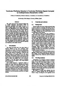
FIG. 1. Nonlinear analysis of a typical RR-interval series. (A) The first 512 points in the interval series {RR(i)} as a function of the interval number i. (B) The lag plot: RR(i + 1) as a function of RR(i), from a series of 1023 RR intervals. No pattern is evident. Applying linear regression yields r2 = 0.02, explaining 2% of the variance in RR(i + 1). (C) Smoothing the lag plot with a 25 point moving average. The smoothed lag plot (black squares plotted over the original lag plot of A) appears nonlinear, especially at shorter RR intervals. (D) Analyzing the smoothed lag plot. Analysis of the above smoothed lag plot is complicated by two factors: overlapping bins and the effects of extreme values upon the mean. The latter problem is readily overcome by replacing means by medians; the former problem by using consecutive, nonoverlapping bins.

We next considered possible nonlinear dynamics. In view of limits on the Takens embedding theorem, analysis was restricted to lag plots in R2. Because these lag plots showed little evident pattern, making it difficult to predict RR(j + 1) from the value of RR(j), we considered the simpler problem of predicting the expected value of RR(j + 1). The expected value E(RR(i + 1) RR(i) = RRo) may be estimated from a suitable average of

physiological variables,

+

1) RR(i) is near RRo}.

[2]

This average may be regarded as a moving average of the lag plot (Fig. 1C), averaging values of RR(i + 1) associated with nearby values of RR(i), irrespective of i. Nonlinearity in smoothed lag plots was measured as follows (Fig. 1D). To facilitate comparison with surrogate data (16), each interval series was truncated to the first 1024 points. Each corresponding set of 1023 pairs {(RR(i), RR(i + 1))} was sorted by ascending order of RR(i), and then divided into nonoverlapping bins of equal width 25. The remaining 23 points, corresponding to the largest RR intervals, were not used in subsequent analysis. A median filter was applied to each bin, yielding a smoothed lag plot in R2. Medians were used instead of means to minimize the effects of outlying values of RR(i + 1). The points in Fig. 1C still represent pairs of

RR interval of the x-axis and the

filter. We next computed correlations between successive residuals (after linear regression) in median-filtered lag plots. Note that residuals were ordered by median RR(i), not by the interval number i. The resulting statistic, r =

{RR(i

an

next RR interval on thex-axis, the latter smoothed by a median

avg(ujuj+D)/avg(uj2)

[3]

is linearly related to the Durbin-Watson statistic (cf. ref. 11). In the absence of nonlinear behavior one expects the residuals to be independent and identically distributed, implying

that

r

0 ± 0.16

(mean

±

SD)

in the

case

of 40 residuals.

Simulation results with random linear models yielded r = -0.045 ± 0.157 (6000 replicates). The difference in means is due to small negative correlations between successive residuals for such random models, as illustrated in Fig. 2. The value of r obtained for each episode was compared with two types of surrogate data (16). The first surrogate data sets were obtained by applying the Fast Fourier Transform (which requires an interval series of length a power of 2), randomizing the phases, and applying the inverse Fast Fourier Transform, the second by simply randomly shuffling the interval series itself. Each such surrogate data set consisted of 200 replicates.



10497

Each episode was then compared with its two corresponding surrogate data sets, and the results were converted to percentile ranks associated with its rvalue. (Histograms of aggregated surrogate data agreed closely with those of simulated random linear models, as did their means (P = not significant, t test) and variances (P = ns, bootstrap methods).

analysis also found significant patterns, based upon the comparisons described above, as shown in Fig. 3. Highly significant differences between experimental and surrogate data (the r-statistic at the 99th percentile, P s 0.01, compared separately with both corresponding surrogate data sets) were found in 8 of 19 episodes of ventricular fibrillation. The r-statistic ranked at or above the 85th percentile in 7 of the remaining 11 episodes. (Comparisons with random linear models yielded similar results: 99th percentile r-statistic in 7 episodes, 98th percentile r-statistic in 1 episode, and 85th or greater percentile r-statistic in 7 of the remaining 11 episodes.) Overall, r = 0.246 ± 0.233 (mean ± SD) significantly different from surrogate models (r = -0.051 + 0.153, P < 10-6, t test) and from random linear models (P < 10-6, t test). Since it can be shown analytically that any stable AR(k) model yields the same statistics as a random model, we have detected significant nonlinear behavior. Although our animal model was designed to maintain stationary dynamics, we also tested for evidence of any nonstationarity in the RR-interval series. Except for a statistically significant but physiologically small change in the mean RR interval over each series (an average decrease of 3.0 ± 7.7 ms), we found little evidence of nonstationarity. Moreover, restricting analysis to the most variable episodes yielded no significant differences in r. Hence, the observed nonlinearity in smoothed lag plots of RR-interval series could not be due to any possible nonstationarity in these data. Further examination of smoothed lag plots found several apparent types of dynamical order, including significant correlations between successive residuals at very short RR intervals (-80 ms) (Fig. 4). Nonlinearity at short RR intervals suggests inadequate time for repolarization. In general our results are consistent with the existence of a variety of distinct forms of nonlinear dynamics in ventricular fibrillation.

RESULTS

DISCUSSION

Smoothed lag plots showed significant linear as well as nonlinear patterns. Linear analysis yielded r2 = 0.239 + 0.177, explaining 24% of the variance in smoothed lag plots, with r2 statistically significant in 16 of 19 episodes. Our nonlinear

We have developed a new approach to the analysis of relatively high-dimensional dynamical systems based upon smoothed two-dimensional lag plots, and used this approach to demonstrate highly significant nonlinear and linear dynamical order

FIG. 2. Correlations among successive residuals in a toy random model. Three consecutive points will almost always form a concave up pattern (as shown) or concave down pattern; both cases yield a negative correlation among (the two) successive residuals.

o

60-

0

ca

4

L~

40

FIG. 3. Experimental data compared with surrogate data. Each experimental r value is compared with surrogate data formed by randomizing the phases in experimental power spectra (left bars) and with surrogate data formed by shuffling experimental time series (right bars). The results are shown as percentile ranks of experimental data as compared with corresponding surrogate data. Grouped bars represent results of several recordings from the same episode of ventricular fibrillation.

10498



A 200-

B

180CD)

E

+ 160-

-

ErC CC

a:

140-

120100

150

200

2! 50

RR(n) (ms)

RR(n) (ms)

C 160-

D 160-

140'O 150E

E

.-

1-

+ 120-

cr

I-,

c

140-

100QAn

1 an _

50

100

150

200

80

120

RR(n) (ms)

160

200

RR(n) (ms)

FIG. 4. Smoothed lag plots from four episodes of ventricular fibrillation. A and B, with rF = 0.425 and r = 0.353 (99th percentile) and r2 = 0.326 and r = 0.674 (99th percentile), respectively, show similar "jumps" in the next RR interval, but at different, sharply different current RR intervals. C (r2 = 0.409 and r = 0.024) shows no discernable nonlinearity. D (r2 = 0.176 and r = 0.435, 99th percentile) demonstrates significant nonlinearity, but of a visibly different form than A and B. For construction of these figures, see Fig. 1 B-D.

in ventricular fibrillation. Two-dimensional lag plots are readily constructed, even from a relatively short time series. However, they may be of little apparent use in predicting the next value of a state variable from its current value in the presence of underlying higher-dimensional dynamics (embedding dimension 2 2). Despite this limitation, in systems with underlying dynamical order, the current value of a single, given state variable may partially determine future dynamics, suggesting smoothing as an approach to detecting determinism in two-dimensional lag plots. Evidence for determinism in ventricular fibrillation had been found recently with different and more complicated techniques (7) reminiscent of "chaos control" (8). Nonlinear behavior in normal humans had been shown (17). Because of the complexity of ventricular fibrillation (2) it may be difficult to characterize the relatively short and noisy RR-interval series, which can be obtained from animal models by these or other methods that focus on local predictability (18, 19). Finally, one can detect quadratic (nonlinear) periodicities in time series with bispectra (and higher order periodicities with correspondingly higher order spectra) (20, 21); however, the calculations appear difficult compared with our method. Our methods do not involve reconstruction of an attractor for an underlying dynamical system x(i + 1) = f(x(i)) with state space {x}, from projections y(i) = p((i)).

[41

Instead, the ergodic behavior that underlies attractor struction (14,15) implies that E(y(i + 1) y(i)

=

recon-

yo) = E(p(x(i + 1)) p(x(i)) = yo).

[5]

We may therefore interpret E(y(i + 1) y(i) = yo) as the state average of y(i + 1) over all states with y(i) = yo. Beacuse the use of state averages replaces attractor reconstruction, our methods can be applied to relatively short time series compared with the dimension of any underlying attractor, perhaps yielding new insights into many physiological phenomena. In essence, we sacrificed predictability by smoothing lag plots to reduce their "dimensionality" to analyze them with simple statistical techniques. However, attractor reconstruction, where possible, would clearly provide a more complete understanding of underlying dynamics. We thank Alan Garfinkel for help in electrogram analysis and George Sugihara for helpful discussions. This work was partially supported by a grant from the Heart Council of Long Island. 1. Damle, R. S., Kanaan, N. M., Robinson, N. S., Ge, Y. Z. & Kadish, A. H. (1992) Circulation 86, 1547-1558. 2. Bayly, P. V., Johnson, E. E., Wolf, P. D., Greenside, H. S., Smith, W. M. & Ideker, R. E. (1993) J. Cardiovasc. Electrophysiol. 4, 533-546. 3. Goldberger, A. L., Bhargava, V., West, B. J. & Mandell, A. J. (1986) Physica D 19, 282-289.

Physiology: Hastings et al. 4. Kaplan, D. T. & Cohen, R. J. (1990) Circ. Res. 67, 886-892. 5. Ruelle, D. & Takens, F. (1971) Commun. Math. Phys. 20, 167-192. 6. Ruelle, D. & Takens, F. (1973) Commun. Math. Phys. 23, 343-344. 7. Witkowski, F. X., Kavanagh, K. M., Penkoske, P. A., Plonsey, R., Spano, M. L., Ditto, W. L. & Kaplan, D. T. (1995) Phys. Rev. Lett. 75, 1230-1233. 8. Garfinkel, A., Spano, M. L., Ditto, W. L. & Weiss, M. (1992) Science 257, 1230-1235. 9. Nwasokwa, 0. N. & Bodenheimer, M. M. (1991) Am. J. Physiol. 260, H486-H498. 10. Smith, L. A. (1988) Phys. Lett. A 133, 283-288. 11. Ruelle, D. (1990) Proc. R. Soc. London A 437, 241-248. 12. Draper, N. & Smith, H. (1991) Applied Regression Analysis (Wiley, New York), 2nd Ed. 13. Sugihara, G. & May, R. M. (1990) Nature (London) 344,734-741.


10499

14. Packard, N. H., Crutchfield, J. D., Farmer, J. D. & Shaw, R. S. (1980) Phys. Rev. Lett. 45, 712-716. 15. Takens, F. (1981) Lect. Notes Math. 898, 366-381. 16. Theiler, J., Eubank, S., Longtin, A., Galdrakian, B. & Farmer, J. D. (1992) Physica D 58, 77-94. 17. Sugihara, G., Allan, W., Sobel, D. & Allan, K. D. (1996) Proc. Natl. Acad. Sci. USA 93, 2608-2613. 18. LeBaron, B. (1994) Philos. Trans. R. Soc. LondonA 348, 397-404. 19. Smith, L. A. (1994) Philos. Trans. R. Soc. LondonA 348,371-381. 20. Hasselman, K., Munk, W. & Macdonald, G. (1963) in Time Series Analysis, SIAM Series in Applied Mathematics, ed. Rosenblatt, M. (Wiley, New York), pp. 125-139. 21. Subba Rao, T. (1992) in Nonlinear Modeling and Forecasting, Proceedings of the Santa Fe Institute Studies in the Sciences of Complexity, eds. Casdagli, M. & Eubank, S. (Addison-Wesley, Redwood City, CA), Vol. 12, pp. 199-226.