The dynamics of a sinusoidally driven pendulum in a repulsive magnetic field is investigated theoretically and experimentally. The experimental data are ...
Nonlinear dynamics of a sinusoidally driven pendulum in a repulsive magnetic field Azad Siahmakoun Department of Physics and Applied Optics, Rose-Hulman Institute of Technology, Terre Haute, Indiana 47803
Valentina A. French Department of Physics, Indiana State University, Terre Haute, Indiana 47809
Jeffrey Patterson Department of Physics and Applied Optics, Rose-Hulman Institute of Technology, Terre Haute, Indiana 47803
~Received 24 July 1996; accepted 24 October 1996! The dynamics of a sinusoidally driven pendulum in a repulsive magnetic field is investigated theoretically and experimentally. The experimental data are acquired using a shaft encoder interfaced to a PC which measures the angular displacement of the pendulum as a function of time. Both the theoretical simulations and the experimental measurements exhibit regions of periodic and chaotic behavior, depending on the system parameters. Amplitude jumps, hysteresis, and bistable states are also observed. The simplicity of the apparatus makes this experiment suitable for an advanced undergraduate laboratory. © 1997 American Association of Physics Teachers.
I. INTRODUCTION In recent years several laboratory experiments demonstrating chaotic motion in a pendulum system have been published.1–6 Experiments using a passive double pendulum1,2 demonstrated that a slight change in the initial release position of the pendulum led to the exponential divergence of the pendulum’s trajectories in a chaotic regime. A driven inverted pendulum3 experiment, in which the driver’s frequency was the control parameter, showed how the power spectrum changed during a transition from periodic to 393
Am. J. Phys. 65 ~5!, May 1997
chaotic motion. A simple pendulum whose pivot executed high frequency vertical oscillations4,5 was used to demonstrate stable inverted states by adjusting the amplitude of the pivot’s motion. A magnetic pendulum6 whose deflection was controlled by the currents in an electromagnet at its tip and three others equally spaced around the pendulum was used for analog demonstrations of first- and second-order phase transitions. In this paper we present the results of an investigation of a driven physical pendulum in a repulsive magnetic field. This field is in opposition to the restoring gravitational force ~see © 1997 American Association of Physics Teachers
393
Fig. 1. Schematic diagram of the physical pendulum and the forces acting on it.
Fig. 1! resulting in a damping of the pendulum’s motion. The system consists of a physical pendulum coupled to a sinusoidally varying driving force, and a pair of magnets, one positioned at the end of the pendulum and the other directly below the pendulum’s vertical position. The poles of the magnets are oriented such that a repulsive force exists between them. This apparatus possesses five control parameters: the frequency and the amplitude of the driver, the vertical separation between the magnets ~z direction!, and the relative position of the magnets in a horizontal plane ~x and y directions!. All of these parameters are experimentally accessible without any modifications to the setup, and they contribute to the rich dynamics of the system. The simplicity of this apparatus coupled with its rich dynamics make it suitable for an advanced undergraduate laboratory experiment. The dynamics of this system is investigated both theoretically and experimentally. In the theoretical aspect of our investigation, we use simple Newtonian physics to derive the equations of motion that describe the dynamics of the system. MATHEMATICA™ is then used to solve these equations for specified initial conditions and system parameters ~frequency of the driver, amplitude of the driver, and magnetic strength of the magnets!. From these solutions, time series and phase space plots are constructed and discussed. These plots exhibit regions of both periodic and chaotic behavior, depending on the parameters of the system. The experimental data are acquired using a shaft encoder interfaced to a PC which measures the angular displacement of the pendulum. These measurements are recorded in the form of time series. By numerically differentiating those time series, phase space plots are constructed. Both periodic and chaotic behaviors are observed, depending on the frequency of the driver and the distance between the two magnets. Amplitude jumps, hysteresis, and bistable states occur for a range of frequencies near the natural frequency of the physical pendulum. In Sec. II, we derive the equations of motion and present the results of theoretical simulations. In Sec. III, we describe the experimental apparatus and the measurements obtained from it. Our conclusions are presented in the final section. II. THEORY A theoretical model is developed considering the four forces acting on the pendulum: the restoring gravitational force, the repulsive magnetic force, the sinusoidal driving 394
Am. J. Phys., Vol. 65, No. 5, May 1997
Fig. 2. ~a! Time series and ~b! phase space plots showing periodic motion for d570 mm. ~c! Time series and ~d! phase space plots showing more complicated periodic orbits when the distance, d, between the magnets is decreased to 66.70 mm. Siahmakoun, French, and Patterson
394
Fig. 3. As the distance d is further decreased, transition to chaos occurs near d566.55 mm. ~a! Time series and ~b! phase space plots showing chaotic motion for d566.55 mm.
force applied by horizontally displacing the pivot, and the damping force. Figure 1 shows a diagram of the pendulum and the forces acting on it. The damping force is assumed to be proportional to the angular velocity of the pendulum, v. The magnets are considered to be point magnets. For simplicity of our theoretical model, we assume that the magnetic force is a repulsive force between two point magnets with an inverse squared dependence on distance, and it is thus a function of the angular displacement of the pendulum u, Fmagnetic5
m 0 m 1m 2 rˆ . 4 p r 2u
~1!
Here, m0 is the permeability of vacuum, m 1 ,m 2 are the pole strengths of each magnet, and r u is the distance between the magnets. As can be seen in Fig. 1, r u 5 A~ L sin u ! 2 1h 2u ,
~2!
h u 5d1L ~ 12cos u ! ,
~3!
where L is the length of the pendulum and d is the minimum separation between the two magnets. The horizontal displacement of the pivot is negligibly small compared to L and h u . Newton’s second law is applied to the rotating rigid body and thus the equation of motion takes the form given below 395
Am. J. Phys., Vol. 65, No. 5, May 1997
Fig. 4. ~a! Time series and ~b! phase space plots for d566.54 mm and initial conditions u~0!50.1 rad, v~0!50, F~0!50. The chaotic attractor is bounded in both positive and negative u regions. ~c! Time series and ~d! space phase plots for d566.54 mm and initial conditions u~0!50.1002 rad, v~0!50, F~0!50. Notice the dramatic change in motion caused by only a slight change in the initial conditions. Siahmakoun, French, and Patterson
395
Fig. 5. For d566.53 mm the pendulum is no longer able to overcome the repulsive magnetic field and the chaotic motion is confined to the positive u values.
I
d 2u 5 dt 2
( ti ,
Fig. 6. As the control parameter d is further decreased to 66.40 mm the pendulum displays periodic motion again. The motion is confined to the positive u values.
~4!
where I is the moment of inertia of the pendulum and (ti is the vector sum of all torques acting on the pendulum and is given by
( ti 5 tgravity1 tdriver1 tdamping1 tmagnetic .
~5!
By combining Eqs. 1–5, we arrive at the equations of motion in the form of a system of coupled differential equations L M L2 v˙ 52 M g sin u 1T driver sin F2 g v 3 2 1
uuu m 0 m 1m 2 L u 4 p r 2u
S
SU
3cos u u u 1arctan 2
hu L sin u
U DD
,
~6!
u˙ 5 v ,
~7!
˙ 5V. F
~8!
Here, M is the mass of the pendulum, g is the gravitational acceleration, T driver is the maximum value of the periodic torque produced by the horizontal displacement of the pivot, F and V are, respectively, the phase and the angular fre396
Am. J. Phys., Vol. 65, No. 5, May 1997
Fig. 7. Equilibrium positions of the pendulum as a function of the minimum separation between the magnets, d. Siahmakoun, French, and Patterson
396
where A, B, C, and D are constant coefficients that depend
only on the physical constants associated with the system. The coupled differential equations ~7!, ~8!, and ~9! are solved numerically using MATHEMATICA. The following parameter values and initial conditions are used for the computer simulations: A5110 s22, B50.01 s22, C50.001 s21, D50.2 m2/s2, u~0!50.1 rad, v~0!50, F~0!50. Data are recorded after allowing the transient behavior of the pendulum to die out ~i.e., after 30 cycles!. While the driver’s frequency is kept constant at 1 Hz both periodic and chaotic behaviors are observed by varying the distance, d, between the two magnets. For example, for values of d between 100 and 70 mm the pendulum exhibits periodic behavior as shown in Fig. 2. As d is decreased further, more complicated orbits are observed @Fig. 2~c! and ~d!# and then transition to chaos occurs near d566.55 mm, as shown in Fig. 3. As can be seen from the time series in Fig. 3~a!, after a few oscillations on both sides of the equilibrium position, the pendulum is no longer able to overcome the repulsive magnetic field and its oscillations are trapped on one side. For d566.54 mm chaotic behavior is observed where the chaotic attractor is bounded in both positive and negative u regions @Fig. 4~b!#. In this case the pendulum is at first momentarily trapped on one side, as shown in Fig. 4~a!, and then it suddenly overcomes the magnetic field, getting trapped on the other side.
Fig. 9. Experimental time series and phase space plots generated by the shaft encoder–PC system showing periodic motion for d570 mm.
Fig. 10. Experimental plots showing transition to chaos as the magnets are moved closer together at a distance d555.60 mm.
Fig. 8. Experimental setup for the study of the dynamics of a sinusoidally driven physical pendulum in a repulsive magnetic field.
quency of the driver, and g is the damping constant. Equation ~6! can be rewritten in a simpler form
v˙ 52A sin u 1B sin F2C v 1
S
SU
3cos u u u 1arctan 2
397
uuu D u r 2u
hu L sin u
U DD
,
Am. J. Phys., Vol. 65, No. 5, May 1997
~9!
Siahmakoun, French, and Patterson
397
Fig. 11. Time series and phase space plots generated from the experimental data showing chaotic behavior for the control parameters: ~a!, ~b! d555.40 mm; ~c!, ~d! d555.30 mm.
Figure 4~c! and ~d! shows the pendulum’s motion for the same distance between the magnets, d566.54 mm, but for slightly different initial conditions: u~0!50.1002 rad, v~0!50, and F~0!50. Notice the dramatic change in the pendulum’s motion caused by only a very slight change in the initial conditions ~i.e., a change of 0.0002 rad '0.01 deg in the initial angular position of the pendulum!. This is an illustration of one of the characteristic features of chaotic motion: its sensitive dependence on initial conditions. Near d566.53 mm, the magnetic field becomes sufficiently large that the pendulum is no longer able to overcome it and the trajectories are confined to the positive u regions ~Fig. 5!. As d is further decreased, a periodic motion confined to the positive u region is observed about a new equilibrium point as shown in Fig. 6. The presence of such equilibrium points can be predicted by solving Eq. ~9! for an unforced pendulum. Figure 7 displays a plot of the equilibrium positions of the pendulum as a function of the minimum separation between the magnets d. Notice that two new equilibrium positions, one on either side of the vertical position, appear as the distance d is decreased below 70 mm. Similar observations are also reported for a magnetoelastic pendulum.7 398
Am. J. Phys., Vol. 65, No. 5, May 1997
III. EXPERIMENT The experimental apparatus, shown in Fig. 8, consists of a physical pendulum made of an aluminum rod 13 cm long and of mass 11.4 g. This rod is mounted on a U.S. Digital softpot ~shaft encoder! model SP-512B such that the pendulum can rotate freely, but the rotation is restricted to a plane. The shaft encoder is used to record angular displacement data via a software package.8 The software package allows immediate viewing of the time series and phase space plots of the pendulum’s motion. The pendulum is coupled to a Pasco Scientific Mechanical Vibrator, model SF-9324, which constitutes the driving force of the pendulum. The amplitude of this mechanical driver is adjustable with a maximum of 5 mm. A sinusoidal signal produced by an SRS synthesized function generator model DS 345 is supplied to the driver. The frequency and amplitude of the driver are varied by changing the frequency and amplitude of the signal produced by the function generator. A disk magnet of mass 5 g and of the same diameter as the aluminum rod is attached to the lower end of the rod. An identical disk magnet is attached to the table directly below the pendulum’s vertical position. Siahmakoun, French, and Patterson
398
Fig. 13. Experimental amplitude curve displaying bistable states for driving frequencies 1.1–1.35 Hz and hysteresis. m points represent the increasing frequency ~forward! path; s points represent the decreasing frequency ~return! path.
Fig. 12. Experimental plots showing chaotic motion for d555.10 mm.
The two magnets are oriented with like poles facing each other. The pendulum is suspended from an aluminum rod which is placed on a three-way precision translation stage so that the separation distance between the two magnets can be varied in steps as small as 10 microns. Starting with the minimum separation between the two magnets as the control parameter, the driver’s amplitude and frequency are kept constant at 5 mm and 1.33 Hz, respectively. All the experimental measurements are taken after the transient behavior of the pendulum is allowed to die out ~after approximately 30 cycles!. Thus the zero on the time scale of the experimental plots does not represent the starting moment of the pendulum motion. The experimental data show similar features of the dynamics that were found in the computer simulations. Figure 9 shows a periodic motion for a distance d of 70 mm. For distances d in the range 56–55 mm, the pendulum displays chaotic motions. Figures 10–12 display the pendulum’s motions at a few distances d in this range. As can be seen from the time series and phase space plots, the pendulum executes a few oscillations on both sides of the vertical equilibrium position, after which it is trapped on one side for a few moments. It then suddenly overcomes the magnetic field and is trapped on the opposite side for a few cycles after which is able to overcome the magnetic field 399
Am. J. Phys., Vol. 65, No. 5, May 1997
again and change sides. This happens when the restoring and driving torques are in step with each other such that the resultant can overcome the repulsive magnetic torque. The pendulum displays now two new equilibrium positions, one on each side of the vertical position, and the orbits change randomly between oscillations about either one of these positions and oscillations about the vertical position. Further decrease in d, however, results in oscillations bounded to one side of the vertical equilibrium as pointed out in Sec. II. Notice the drastic change in the pendulum’s trajectories produced by only a small change in the distance d. All these features are also found in the computer simulations ~see Figs. 2–7!. Using the same experimental setup we are also able to study amplitude jumps and hysteresis. The angular amplitude of the pendulum is plotted as a function of the frequency of the driver, while the driver’s amplitude is kept at its maximum value and the distance between the two magnets is kept constant at 70 mm. A hysteresis curve is obtained, as shown in Fig. 13. Similar observations are also reported for an inverted pendulum.9 Notice that the amplitude of oscillation increases continuously as the frequency increases ~m data points! up to a frequency of 1.35 Hz. At this point the amplitude drops discontinuously from 0.59 to 0.03 rad. After this point a continuous decrease in amplitude is observed as the driving frequency is increased. The frequency is then decreased through the same range starting from 1.5 Hz ~s data points constitute the return path!. At first the amplitude increases following the lower branch of the return curve. When the decreasing frequency reaches a value of 1.1 Hz, there is a second discontinuous jump in amplitude from 0.08 to 0.18 rad. After 1.1 Hz the amplitude decreases continuously with decreasing frequency as shown in Fig. 13. The above results lead to two observations: ~1! for driving frequencies between 1.1 and 1.35 Hz the amplitude curve is bistable; ~2! the amplitude of the pendulum is dependent not only on the range of the driving frequencies but also on the history of that frequency range. Siahmakoun, French, and Patterson
399
IV. CONCLUSIONS The physical pendulum in a repulsive magnetic field presented here is a system that exhibits rich nonlinear dynamics. Periodic and chaotic behaviors are investigated for different values of the control parameters ~driver frequency and minimum separation between two magnets!. The characteristic sensitive dependance of the pendulum’s chaotic motion on the initial conditions is also demonstrated. Also presented here are the characteristic features of nonlinear systems such as bistable states, amplitude jumps, and hysteresis. The experimental data are acquired in real time using a shaft encoder–PC system. The plots generated from these data exhibit the same features as those predicted by the theoretical simulations. The experimental setup has up to five control parameters that are experimentally accessible in real time: the frequency and the amplitude of the driver, the minimum separation between the magnets, and the relative position of the magnets in a horizontal plane. The system holds much promise for further studies since not all of the above control parameters are examined in this paper. Furthermore, the ex-
400
Am. J. Phys., Vol. 65, No. 5, May 1997
perimental setup is simple and inexpensive to build, making it a suitable and affordable experiment for an advanced undergraduate physics laboratory. 1
T. Shinbrot, C. Grebogi, J. Wisdom, and J. A. Yorke, ‘‘Chaos in a double pendulum,’’ Am. J. Phys. 60, 491–498 ~1992!. 2 R. B. Levien, and S. M. Tan, ‘‘Double pendulum: An experiment in chaos,’’ Am. J. Phys. 61, 1038–1044 ~1993!. 3 B. Duchesne, C. W. Fischer, C. G. Gray, and K. R. Jeffrey, ‘‘Chaos in the motion of an inverted pendulum: An undergraduate laboratory experiment,’’ Am. J. Phys. 59, 987–992 ~1991!. 4 H. J. T. Smith, and J. A. Blackburn, ‘‘Experimental study of an inverted pendulum,’’ Am. J. Phys. 60, 909–911 ~1992!. 5 James A. Blackburn, H. J. T. Smith, and N. Gronbech-Jensen, ‘‘Stability and Hopf bifurcations in an inverted pendulum,’’ Am. J. Phys. 60, 903– 908 ~1992!. 6 V. H. Schmidt, and B. R. Childers, ‘‘Magnetic pendulum apparatus for analog demonstration of first-order and second-order phase transitions and tricritical points,’’ Am. J. Phys. 52, 39–43 ~1984!. 7 F. C. Moon and P. J. Holmes, ‘‘A magnetoelastic strange attractor,’’ J. Sound Vib. 65, 275–296 ~1979!. 8 Trevis J. Litherland, and Azad Siahmakoun, ‘‘Chaotic behavior of the Zeeman Catastrophe Machine,’’ Am. J. Phys. 63, 426–431 ~1995!. 9 N. Alessi, C. W. Fischer, and C. G. Gray, ‘‘Measurement of amplitude jumps and hysteresis in a driven inverted pendulum,’’ Am. J. Phys. 60, 755–756 ~1992!.
Siahmakoun, French, and Patterson
400