The rate of growth of the nonlinear terms in the vorticity equation are analysed for a turbulent flow with r.m.s. velocity u0 and integral length scale L subjected to.
333
J. Fluid Mech. (1997), vol. 337, pp. 333–364 c 1997 Cambridge University Press Copyright
Nonlinear interactions in turbulence with strong irrotational straining By N. K. - R. K E V L A H A N1
AND
J. C. R. H U N T 2
´ LMD-CNRS, Ecole Normale Sup´erieure, 24 rue Lhomond, 75231 Paris Cedex 05, France Department of Applied Mathematics and Theoretical Physics, University of Cambridge, Silver Street, Cambridge, CB3 9EW, UK 1
2
(Received 23 May 1996 and in revised form 10 December 1996)
The rate of growth of the nonlinear terms in the vorticity equation are analysed for a turbulent flow with r.m.s. velocity u0 and integral length scale L subjected to a strong uniform irrotational plane strain S, where (u0 /L)/S = � � 1. The rapid distortion theory (RDT) solution is the zeroth-order term of the perturbation series solution in terms of �. We use the asymptotic form of the convolution integrals for the leading-order nonlinear terms when β = exp(−St) � 1 to determine at what time t and beyond what wavenumber k (normalized on L) the perturbation series in � fails, and hence derive the following conditions for the validity of RDT in these flows. (a) The magnitude of the nonlinear terms of order � depends sensitively on the amplitude of eddies with large length scales in the direction x2 of negative strain. (b) If the integral of the velocity component u2 is zero the leading-order nonlinear terms increase and decrease in the same way as the linear terms, even those that decrease exponentially. In this case RDT calculations of vorticity spectra become invalid at a time tNL ∼ L/u0 k −3 independent of � and the power law of the initial energy spectrum, but the calculation of the r.m.s. velocity components by RDT remains accurate until t = TNL ∼ L/u0 , when the maximum amplification of r.m.s. vorticity is ω/S ∼ � exp(�−1 ) � 1. (c) If this special condition does not apply, the leadingorder nonlinear terms increase faster than the linear terms by a factor O(β −1 ). RDT calculations of the vorticity spectrum then fail at a shorter time tNL ∼ (1/S) ln(�−1 k −3 ); in this case TNL ∼ (1/S) ln(�−1 ) and the maximum amplification of r.m.s. vorticity is ω/S ∼ 1. (d ) Viscous effects dominate when t � (1/S) ln(k−1 (Re/�)1/2 ). In the first case RDT fails immediately in this range, while in the second case RDT usually fails before viscosity becomes important. The general analytical result (a) is confirmed by numerical evaluation of the integrals for a particular form of eddy, while (a), (b), (c) are explained physically by considering the deformation of differently oriented vortex rings. The results are compared with small-scale turbulence approaching bluff bodies where � � 1 and β � 1. These results also explain dynamically why the intermediate eigenvector of the strain S aligns with the vorticity vector, why the greatest increase in enstrophy production occurs in regions where S has a positive intermediate eigenvalue; and why large-scale strain S of a small-scale vorticity can amplify the small-scale strain rates to a level greater than S – one of the essential characteristics of high-Reynoldsnumber turbulence.
334
N. K.-R. Kevlahan and J. C. R. Hunt
1. Introduction In most turbulent flows the large-scale velocity field is a straining motion, either irrotational or rotational, that changes slowly on the time scale of the turbulent eddies – for example flow over waves, turbulence entering engines etc. The main practical and fundamental question concerns how the statistical and eddy structure of the turbulence is distorted by the strain and how its other properties are changed, such as mixing caused by the separation of fluid elements, or dissipation caused by transfer of kinetic energy to small scales. A key problem of turbulence research is to study how the nonlinear interaction between eddies or between Fourier components is affected by distortion. It is now well known that many aspects of distorted turbulent flows are determined by the linear interaction between the turbulence and the large-scale mean straining flow and for which the nonlinear interaction can be neglected (see the review by Hunt & Carruthers 1990). Rapid distortion theory (RDT) is the term used to describe these methods and detailed assumptions of this simplified, though where appropriate quite powerful, approach. The only theoretical calculations of the nonlinear interaction for turbulent flows have been based on statistical physics concepts, such as direct interaction approximation (DIA) and eddy-damped quasi-normal Markovian (EDQNM) (reviewed recently by McComb 1990). Cambon & Jacquin (1989) and Cambon, Mansour & Godeferd (1997) have extensively investigated the effects of rotation on turbulent flow using EDQNM, and have developed weakly nonlinear theories which relate EDQNM to RDT. It has not been shown how and when the nonlinear interaction dominates linear distortion effects in the case of irrotational strain, and therefore we do not have much understanding of the limitations of RDT. In this paper we explore a different approach based on a general asymptotic analysis of the nonlinear terms (expressed in terms of convolution of Fourier transforms) for the fluctuating vorticity field; no assumptions are made about its initial form provided its amplitude is small compared with the mean strain. This allows us to calculate the next term in the expansion of which RDT is the zeroth-order term, and hence to estimate accurately the period of validity of RDT. The changes in the form of the eddy structure under the action of an irrotational plane strain were defined with more precision using topological and kinematic concepts by Hunt & Kevlahan (1994). That study provides further evidence that the analysis of the nonlinear term associated with these linearly distorted structures should provide a first-order estimate for the limitations of the linear calculation. The work presented here may well provide a general approach for estimating nonlinear effects in a wide range of distorted turbulent flows; and perhaps also a new method for improving the nonlinear ‘pressure–strain’ terms in the model equation for turbulent Reynolds stress (recently reviewed by Launder 1989). The nonlinear terms in the equation for the fluctuating vorticity ω when the turbulence is undergoing a large-scale plane strain U (x) are those representing the vortex lines being randomly rotated and stretched (by the terms (ω ·∇)u) and advected (by the term (u · ∇)ω) by the small-scale turbulence u. The approach hitherto for estimating the nonlinear terms relative to the linear terms (ω ·∇)U has been to assume either that (ω · ∇)u has the same value as in undistorted turbulence (∼ (u(l)2 /l 2 )t=0 ), in which case the nonlinear terms are always greater than any exponentially decreasing linear term, or that the magnitude of (ω · ∇)u is determined by the maximum value of ω and u in the distorted flow in which case (ω · ∇)u could grow even faster than
Nonlinear interactions in strained turbulence
335
the fastest growing linear term. Neither of these cases is likely because, as seen in the numerical simulation of Marshall & Grant (1994), the eddy structure changes in such a way as to reduce the nonlinear vorticity distortion terms! In the most frequently used current Reynolds stress models, these nonlinear terms are based on estimates of the local distorted value of the turbulence covariance components and not on the distorted eddy structure. However the latter point has been demonstrated as crucial in modelling the nonlinear rotating and stretching effect, through an idealized analysis of large-scale and small-scale turbulence undergoing distortion (Kida & Hunt 1989). In this paper we analyse in detail the distortion of turbulence caused by a largescale irrotational plane straining flow, because of its importance in a number of engineering problems and because of its fundamental importance in developing the basic theory of turbulence structure. In §2 we review the classical assumptions about the RDT approximation and present the viscous RDT equations and solutions for irrotational plane strain. We then calculate the neglected nonlinear terms (using the RDT solutions) for general initial conditions in §3, using asymptotic analysis for large total strain to determine how these terms evolve over time. These zeroth-order nonlinear terms are then used to calculate the next-order term in the RDT expansion. We make the interesting discovery that the RDT assumptions can remain valid for a relatively long time, usually until the final period of viscous decay, provided that the integral of the initial turbulent velocity in the compressed direction is zero. This condition is satisfied, for example, by eddies aligned in the compressed direction. Estimates of the validity time of RDT are made and compared to the classical results. Finally, in §4, the analytical results are verified against numerical calculations of the nonlinear terms for the Townsend eddy, and explained by simple calculations of the deformation of vortex rings. In the second part (§5) of this paper we relate our results on the validity of RDT to highly localized dynamical processes that occur within particular types of eddy structure in direct numerical simulations (DNS). Two questions arise naturally from these observations. First, which of these results are related to the internal dynamics of the structures, and which to interactions between these structures and the largescale motions around them? Secondly, what is the dynamical explanation for this intermittency and the generation of persistent coherent structures? These questions are investigated here using the linear dynamical approach of RDT. More specifically, we try to determine which aspects of ‘real’ turbulence that are not present in random or Gaussian velocity fields also appear when Gaussian velocity fields are subjected to rapid irrotational strain. A striking observation whose dynamical origin is unclear is the alignment between the intermediate eigenvector (associated with the intermediate eigenvalue) of the rate-of-strain tensor and the vorticity. This alignment is not observed in Gaussian or random turbulence (Shtilman, Spector & Tsinober 1993). Ashurst et al. (1987), Vincent & Meneguzzi (1991) and Blackburn, Mansour & Cantwell (1996) observe such an alignment in DNS and it has been suggested that it may arise from nonlinear effects. Recently Jim´enez (1992) has put forward a theory to explain why one might expect to see the alignment between the vorticity and the intermediate eigenvector of the rate of strain tensor in regions where the vorticity is aligned primarily in one direction (a ‘vortex tube’ or ‘vortex sheet’). The dynamical result we obtain here which shows how a vortex sheet (and hence the observed alignment) is produced by persistent irrotational straining of initially random and isotropic small scales complements Jim´enez’s kinematical explanation.
336
N. K.-R. Kevlahan and J. C. R. Hunt
We also demonstrate how the difference in enstrophy production between regions with positive and negative intermediate eigenvalues of the rate-of-strain tensor, which was derived heuristically by Betchov (1956), might develop.
2. RDT equations and assumptions 2.1. Rapid distortion equations The vorticity and associated velocity equations for an incompressible flow, for a fluid with uniform properties and with no rotational body forces, are
and
∂2 Ωi ∂Ωi ∂Ui ∂Ωi + Uj = Ωj +ν , ∂t ∂xj ∂xj ∂xj ∂xj ∂Uj = 0, ∂xj
(2.1) (2.2)
where Ui is the velocity field and Ωi is the vorticity field, where Ωi = �ijk ∂Uk /∂xj so that ∂Ωk /∂xk = 0. We now divide the vorticity and velocity fields into mean and turbulent parts, Ui = U¯ i + ui , Ωi = ωi where we have assumed that the mean flow is irrotational. We further assume that the mean velocity field U¯ i is a uniform strain U¯ i (xj , t) = Sij (t)xj + U¯ 0i (t),
(2.3)
and represent the turbulent parts as the superposition of plane waves using Fourier transforms Z ˆ i (χ, t) exp(iχ(t) · x) dχ(t), (2.4) ωi (x, t) = ω Z χj (t) ˆ k (χ, t) exp(iχ(t) · x) dχ(t). ω ui (x, t) = i�ijk (2.5) χ(t)2 By applying the principle of the conservation of wavefronts to these weakly nonlinear flows χi (t) varies in time according to dχi (t) = −Sji (t)χj . (2.6) dt This eliminates any explicit dependence on physical space positions xi when we make the substitutions (2.4) and (2.5) in (2.1). If we make the above substitutions we obtain the following equations for the ˆ i: evolution of ω ˆi dω ˆ i (ω, ˆi +Q ˆ j Sij − νχ2 ω ˆ χ), =ω (2.7) dt ˆ i (ω, ˆ χ) is the term nonlinear in turbulent quantities and is defined as where Q χk χj χk ˆ i (ω, ˆ l ∗ χj ωˆ i − ω ˆ l, ˆ χ) ≡ �jkl 2 ω ˆ j ∗ �ikl 2 ω Q (2.8) χ χ where ∗ signifies convolution. The first term on the right-hand side of (2.8) is the nonlinear advection and the second is the nonlinear vortex stretching. The RDT ˆ i ≡ 0 in (2.7) which linearizes the equations and equations are obtained by putting Q allows analytical solutions in a number of cases (e.g. irrotational strain, pure shear and axisymmetric strain). It is appropriate at this point to note the similarities between classical hydrodynamic stability theory and RDT. In stability theory one expresses the perturbation in terms
Nonlinear interactions in strained turbulence
337
of wavy modes which have the prescribed form exp(i(kj xj − σ(k)t)) where the solution for σ indicates whether the perturbed modes oscillate or grow exponentially. In RDT, on the other hand, the perturbation (in this case the turbulence) is represented in terms of distorted Fourier modes exp(iχj (t)xj ). (For the early origins see Craik & Criminale 1986.) These distorted Fourier modes are more complicated than the wavy modes and allow a richer description of the development of the turbulence. In the next section we consider the conditions for the validity of the rapid distortion approximation: the turbulent quantities are much smaller than the mean quantities so that the nonlinear terms can be ignored. Note that if the turbulent part of the flow is made up of a single plane wave then the nonlinear terms in the form of convolutions become products which are identically zero due to the incompressibility ˆ j = 0 and χj uˆ j = 0. relations χj ω 2.2. RDT assumptions The conditions for RDT are usually defined for eddies of length scale l and velocity scale u(l) undergoing some kind of distortion over a time TD , where the distortion may be an imposed strain of strength S, the sudden introduction of a boundary (in the frame of reference moving with the mean flow) or body forces etc. RDT is stated to be valid either if TD is so rapid that the nonlinear terms in the vorticity equation (2.7) have a negligible effect on the vorticity of the eddy (∼ u(l)/l) on the relevant time scale τ(l) of the eddy l/u(l), or if the linear effects on ω of the distortion (e.g. ∼ S(u/l) for a straining distortion) are much stronger than the nonlinear self-induced straining by the turbulence (∼ (u/l)2 ). This leads to two possible conditions for RDT: TD � τ(l) ∼ l/u(l)
or S � u(l)/l.
(2.9a, b)
The latter condition for the strength of the strain rate may be satisfied even when the distortion is applied over a long period, i.e. for slowly changing turbulence, and may be a valid condition for the accurate use of RDT. Hence in any given context one must take care to define precisely the term ‘RDT’. Note that the condition (2.9a) is only satisfied for small values of TD and (2.9b) for larger values of S. Since the time scale l/u(l) decreases as l decreases in most observed turbulent flows, it follows that the nonlinear terms are more significant for smaller eddies. An overall criterion for the validity of RDT for calculating the statistics of the energy-containing eddies in a given turbulent flow can be derived from (2.9) in terms of the r.m.s. velocity u0 and the integral time scale TL . This leads to TD � TL ∼ L/u0
or (u0 /L)/S = � � 1,
(2.10a)
which can be re-expressed as 1/TL � max(S, 1/TD ).
(2.10b)
This criterion determines whether RDT should be a valid approximation at the start of the distortion. But, since (2.10b) does not indicate how long (and completely) the RDT approximation will hold if S � 1/TL , the condition on the applied strain gives no time limit. The central purpose of this paper is to deduce estimates of the period of validity of RDT calculations over wavenumber space and for different components of the velocity and vorticity. Hunt & Carruthers (1990) pointed out that in slowly distorted flows, even when
338
N. K.-R. Kevlahan and J. C. R. Hunt Parallel flow
x2 U
Constant rate of strain
Parallel flow
x1 x3
Figure 1. Schematic diagram of a laterally distorting wind tunnel producing a constant positive rate of strain in the horizontal direction and an equal negative rate of strain in the vertical direction (after Tucker & Reynolds 1968).
neither criterion in (2.10b) is satisfied, RDT calculations often describe the main features of turbulence. As explained in the introductory section, these conditions have been derived from the vorticity equation by inspection, and by assuming that the nonlinear terms are of the same order as in the undistorted turbulence. However, where the turbulence is strongly distorted the nonlinear stretching term (ω · ∇)u can be much less than the undistorted estimate of (u(l)/l)2 , a good example being where the distorted flow forms into strong straight vortex tubes where vorticity is greater than the applied strain rate S; in this case the nonlinear vortex stretching term vanishes identically. The criteria (2.9), (2.10) are only applicable when the linear approximation to the vorticity equation is used to calculate the statistics of the velocity field (and not, for example, the vorticity variance) (see Hunt & Carruthers 1990 and §3 in this paper). Note that viscous stresses can be neglected for those eddy scales whose viscous decay time scale is much longer than the distortion time TD , or than the strain time scale S −1 , i.e. (l 2 /ν) � max(S −1 , TD ).
(2.10c)
If the applied strain is irrotational, the effect of viscosity (or an eddy viscosity for small-scale effects) is merely to add an identical exponential decay factor to all terms of the rate of strain tensor of the turbulence velocity ∂ui /∂xj , and hence does not affect the relative alignment of ω and u. 2.3. Irrotational plane strain Before considering irrotational strain it is helpful to recall the basic types of plane strain and the behaviour of the RDT solutions in each case (see also Townsend 1976 or Cambon et al. 1994 for more details). Plane strain may be divided into three classes: hyperbolic (strain dominates), shear (strain equals rotation) and elliptic (rotation dominates). In the hyperbolic case (of which irrotational strain is the limit) the RDT solutions have exponential growth, in the shear case the RDT solutions have algebraic growth, and in the elliptical case the solutions consist of non-amplified inertial waves except in a narrow band of wave-vectors where the solution grows exponentially. Pure rotation has no such elliptical flow instability so that only dispersive inertial waves exist. Thus the analysis presented in this paper of the growth of nonlinear terms in
Nonlinear interactions in strained turbulence
339
the case of irrotational strain should be representative of hyperbolic strain, but one should expect quite different results in the case of shear or elliptic strain. In this paper we focus on the case of steady plane irrotational (or pure) strain that is uniform on the scale of the turbulent eddies. This idealized flow is relevant to the straining of the smaller-scale eddies by large-scale motion in fully developed turbulence since velocity gradients are formally a superposition of pure straining motion and pure rotation. The transfer of energy to the small scales is greater in the pure strain regions; our model calculation allows for weak nonlinear effects and thus provides more detailed insight into this process than the pure RDT calculation (Townsend 1976, pp. 99–100, and Kida & Hunt 1989). This problem is of direct interest in the distortion of small-scale turbulence by a bluff body (Hunt 1973). Plane irrotational distortion can be easily produced in the laboratory using the type of wind-tunnel set-up shown schematically in figure 1 and thus we can easily compare our results with experiment. Finally, the RDT vorticity and wave-vector solutions are particularly simple in the case of irrotational strain. We will assume that the turbulence has no effect on the straining flow, and for simplicity S is taken as a constant (although the calculation can be generalized to varying strain). In this case the deformation tensor Sij (t) becomes S 0 0 Sij (t) = Sij = 0 −S 0 . (2.11) 0 0 0 ˆ i (χ, t) becomes Equation (2.7) for the evolution of the Fourier transform of vorticity ω ˆ1 dω ˆ 1 (ω, ˆ1 +Q ˆ 1 − νχ2 ω ˆ χ), = Sω dt ˆ2 dω ˆ 2 (ω, ˆ2 +Q ˆ 2 − νχ2 ω ˆ χ), = −S ω dt where the nonlinear terms are χj χk ˆ 1 (ω, ˆ 2 − χ2 ω ˆ 3 ) + �jkl 2 ω ˆ l ∗ χj ω ˆ 1, ˆ χ) = ω ˆ j ∗ 2 (χ3 ω Q χ χ χj χk ˆ 2 (ω, ˆ 3 − χ3 ω ˆ 1 ) + �jkl 2 ω ˆ l ∗ χj ω ˆ 2, ˆ χ) = ω ˆ j ∗ 2 (χ1 ω Q χ χ
(2.12a) (2.12b)
(2.13a) (2.13b)
ˆ 3 may be found from the solenoidal relation and ω ˆ 1 + χ2 ω ˆ 2 + χ3 ω ˆ 3 = 0. χ1 ω
(2.14)
The wave-vector equation (2.6) has the solutions χ1 (t) = k1 exp(−St),
χ2 (t) = k2 exp(St),
χ3 (t) = k3 ,
(2.15a–c)
where k is the wave-vector at t = 0. ˆ i (χ) and χ by the initial integral scale L Non-dimensionalizing the equations for ω and the initial r.m.s. turbulence velocity u0 , (2.12) and (2.15) become � � ˆ1 1 2 dω 1 ˆ 1 (ω, ˆ χ), ˆ1 +Q = − χ ω dt � Re � � ˆ2 1 2 dω 1 ˆ 2 (ω, ˆ χ), ˆ2 +Q =− + χ ω dt � Re χ1 (t) = k1 exp(−t/�),
χ2 (t) = k2 exp(t/�),
χ3 (t) = k3 ,
340
N. K.-R. Kevlahan and J. C. R. Hunt
where � = (u0 /L)/S � 1 is the ratio of the strain rate of the energy-containing turbulence eddies to the applied strain rate, Re = u0 L/ν is the Reynolds number, and ˆ i , χi , ki and t are now non-dimensional. Note that because the ratio the quantities ω of the integral scale to the dissipation scale in high-Reynolds-number turbulence is approximately Re3/4 the wavenumber range for which there is significant turbulent energy is 0 6 ki . Re3/4 .
(2.16)
Because we are interested in long-time St � 1 solutions (where t is the original dimensional time), we make the change of variables τ = t/� in the dimensionless equations, and the RDT equations become ˆ1 � � 2� dω ˆ 1 (ω, ˆ χ), ˆ 1 + �Q = 1− χ ω (2.17a) dτ Re � ˆ2 � 2� dω ˆ 2 (ω, ˆ 2 + �Q ˆ χ), =− 1+ χ ω (2.17b) dτ Re χ1 (τ) = k1 exp(−τ),
χ2 (τ) = k2 exp(τ),
χ3 (τ) = k3 .
(2.18a–c)
Making the zeroth-order, or RDT, approximation implies neglecting the nonlinear terms which are order � (but keeping the viscous terms) and leads to the solution ˆ 10 (k)fˆν1 (k, β), ˆ 1 (k, β) = β −1 ω ω ˆ 2 (k, β) = β ω ˆ 20 (k)fˆν1 (k, β), ω
(2.19a)
ˆ 3 (k, β) = ω ˆ 30 (k)fˆν1 (k, β), ω
(2.19c)
(2.19b)
ˆ i (k) are the initial vorticity components, where the ω β = exp(−τ) is the inverse of the strain ratio c, n � � �o k12 (1 − β 2 ) + k22 (β −2 − 1) + k32 ln(β −2 ) fˆν1 (k, β) = exp − 2Re
(2.20)
(2.21)
is the viscous decay factor, and we have expressed the results in terms of (k, β) rather than (χ(t), t) for simplicity. Thus, in the inviscid range when β 2 � k 2 �/Re the vorticity component in the stretching direction of the applied strain increases exponentially, while the vorticity component in the compressing direction decreases exponentially. The vorticity component normal to the plane of the applied strain is unaffected. The problem to be addressed in the next section is calculating the next term in the asymptotic expansion in terms of � and determining the value of β at which the expansion becomes singular. Note that the distorted velocity field and its statistics can be derived from the expressions (2.19a) to (2.19c) in the RDT limit. The variances were first calculated by Batchelor & Proudman (1954); asymptotic properties of the spectra were derived ˆ and uˆ have been obtained for other by Hunt (1973). Note that exact solutions for ω basic strain motions (axisymmetric, shear, rotational), but not for all types (Cambon 1982; Craik & Criminale 1986). In the analysis of this paper it is assumed that the turbulence scale is much less than the scale over which ∇u varies. When the turbulence scales are large, RDT can still be used, but different analytical techniques are required.
341
Nonlinear interactions in strained turbulence
3. Growth of nonlinear terms 3.1. The general perturbation problem The RDT solutions are exact solutions of the Navier–Stokes equations if the initial flow is a single plane wave because in this case the nonlinear terms are exactly zero (Craik & Criminale 1986). Real turbulence, however, consists of a continuous spectrum of plane waves which interact nonlinearly. So the RDT approach is only accurate when the nonlinear terms are relatively small. We might expect that the RDT approximation eventually fails because the nonlinear terms grow faster than the linear RDT terms. The order of magnitude estimates given in (2.9) provide a rough guide, but we can find a more precise estimate of the period of validity for RDT by actually calculating the way the nonlinear terms change with time. Formally the following calculation is an evaluation of the first-order term in the expansion in � derived from (2.17). ˆ i (k, τ) in powers of �, Expand ω ˆ i (k, τ) = ω ˆ i(0) (k, τ) + �ω ˆ i(1) (k, τ) + O(�2 ), ω ˆ i(0) . Thus the nonlinear terms become where the RDT solution corresponds to ω ˆ i (ω, ˆ (0) ˆ k, τ) = Q ˆ (0) , k, τ) + O(�). Q i (ω ˆ (1) to the RDT approximation is the solution of the The first-order correction ω equations ˆ 1(1) (k, τ) � � 2 � (1) dω ˆ (0) (ω ˆ 1 (k, τ) + Q ˆ (0) , k, τ), = 1− χ (τ) ω (3.1a) 1 dτ Re � ˆ 2(1) (k, τ) � 2 � (1) dω ˆ (0) (ω ˆ 2 (k, τ) + Q ˆ (0) , k, τ). =− 1+ χ (τ) ω (3.1b) 2 dτ Re Thus the first-order correction to the RDT solution can be found by working out the nonlinear terms using the zeroth-order RDT solutions. From the RDT solution (2.18a) to (2.19c), for β � 1 the nonlinear terms in (2.17) can be expressed as Z Z Z ˆ 1(0) (k, β) ∞ ∞ ∞ ω (0) ˆ (0) (ω ˆ 10 (k − k0 )k10 k20 ω ˆ 30 (k0 ) ˆ , k, β) = −β 2 ω Q 1 ˆ 10 (k) −∞ −∞ −∞ ω 0 ˆ 20 (k − k0 )k22 ω ˆ 30 (k0 ) − β 2 ω ˆ 30 (k − k0 )k10 k30 ω ˆ 30 (k0 ) −β 2 ω ˆ 30 (k0 ) + (k2 − k20 )ω ˆ 10 (k0 ) ˆ 10 (k − k0 )k20 ω ˆ 10 (k − k0 )k30 ω +β 2 (k1 − k10 )ω � fˆν2 (k, k0 , β) 0 ˆ 10 (k0 ) 4 0 2 ˆ 10 (k − k0 )k20 ω (3.2a) + (k3 − k30 )ω 0 0 dk β k1 + k22 + β 2 k32 and ˆ 2(0) (k, β) ω (0) ˆ (0) (ω ˆ Q , k, β) = 2 ˆ 20 (k) ω
Z
∞
Z
∞
Z
∞
ˆ 10 (k0 ) ˆ 10 (k − k0 )k10 k30 ω −ω −∞ −∞ −∞ 0 ˆ 10 (k0 ) − ω ˆ 10 (k0 ) ˆ 30 (k − k0 )k32 ω ˆ 20 (k − k0 )k20 k30 ω −ω 0 0 0 2 0 ˆ 30 (k ) + (k2 − k20 )ω ˆ 20 (k − k )k2 ω ˆ 20 (k +β (k1 − k1 )ω 0 � fˆν2 (k, k , β) 0 ˆ 20 (k0 )k20 ω ˆ 10 (k0 ) 4 0 2 + k30 ω 0 0 dk , β k1 + k22 + β 2 k32
ˆ 10 (k0 ) − k0 )k30 ω (3.2b)
ˆ i(0) (k, β) are the RDT solutions, ω ˆ i0 (k) are the initial Fourier transformed where ω
342
N. K.-R. Kevlahan and J. C. R. Hunt
vorticity components, and when β � 1, n � h 0 io 0 0 fˆν2 (k, k0 , β) = exp − (k12 − k1 k10 ) + (k22 − k2 k20 )β −2 + (k32 − k3 k30 ) ln(β −2 ) . Re (3.3) To determine how the magnitude and form of the integrals in (3.2a) and (3.2b) change when total strain is large, i.e. β → 0, we need to find the asymptotic behaviour of integrals of the basic form Z ∞Z ∞Z ∞ ˆ k0 )fˆν2 (k, k0 , β) 0 g(k, (3.4) dk I(k, β) = 02 4 02 2 02 −∞ −∞ −∞ β k1 + k2 + β k3 ˆ i0 (k − k0 )ω ˆ j0 (k0 )kl km for different i, j, l, m. Note that g(k, ˆ k0 ) ˆ k0 ) ∼ ω for β � 1 and g(k, is a non-singular function. An examination of (3.3) or (2.17) immediately shows that, since k = |k| > k2 , there are two time scales to the problem: the inviscid range � � �1/2 k � β � 1, (3.5) Re and the viscous range � � �1/2 . (3.6) β�k Re Therefore, using (2.16), if we want all turbulence scales to be in the inviscid range for a significant time we need � � Re−1/2 .
(3.7)
We consider these two ranges separately below. 3.2. Inviscid range In the inviscid range the convolution integrals for the nonlinear terms have the form of equation (3.4), but with the function fˆν2 replaced by fˆν2 (k, k0 , β) = 1.
(3.8) 2
The largest contribution to the denominators, 1/χ , in (3.4) comes from the region in wavenumber space where k20 = O(β) using standard methods for asymptotics of integrals (e.g. Fraenkel 1969). The integral in the k20 -direction can be found by calculating only the asymmetric part of the integral, i.e. Z ∞ ˆ k0 ) h(k, 0 0 0 0 dk , β 4 k12 + k22 + β 2 k32 2 0 ˆ k0 ) = g(k, ˆ k0 ) + g(k, ˆ −k0 ), and splitting the integral into two ranges from where h(k, 0 0 k2 = 0 to k2 = δ and from k20 = δ to k20 = ∞, i.e. ‘local’ and ‘global’ contributions; the arbitrary transition value δ lies in the range β � δ � 1. To approximate the integral over the small range from 0 to δ we use the rescaling k20 = βK (where K = O(1)) and expand the integrand for small β � Z δ/β � Z δ ˆ k0 ) dk 0 ˆ β2K 2 h(k, 2g(0) 2 −1 4 4 2 1 ˆ 00 = β + (0) + O(β , β K ) dK, h 02 2 4 02 2 02 K2 + C2 K2 + C2 0 β k1 + k 2 + β k3 0 (3.9) 0 0 0 2 0 0 ˆ ˆ ˆ = g(k; k10 , 0, k30 ) and hˆ 00 (0) = ∂2 h/∂k (k; k , 0, k ). Evaluatwhere C 2 = β 2 k12 + k32 , g(0) 2 1 3
Nonlinear interactions in strained turbulence ing the above integral gives � � �� � � β −1 δ δ 1 ˆ 00 ˆ 2g(0) arctan + 2 h (0) δ − Cβ arctan + O(βδ 3 ). C βC βC
343
(3.10)
We can now expand all the terms for large δ/β and collect together terms of similar order with δ = O(β 1/2 ): � � 1 C 2β2 π 1 ˆ 00 ˆ ˆ ˆ ˆ − 2g(0) + 2g(0) g(0) + 2 h (0)δ − g(0)πCβ + O(β 3/2 ). (3.11) Cβ δ 3δ 3 To calculate the integral over the remainder of the range from δ to ∞ we expand the denominator of the integrand for small β as k20 > δ � β: ! Z ∞ Z ∞ ˆ 0 ˆ k0 ) ˆ k0 ) ) h(k, h(k, h(k, k 0 − C 2 β 2 + O(C 4 β 4 ) dk20 . (3.12) 0 0 0 dk = 0 0 β 4 k12 + k22 + β 2 k32 2 k22 k24 δ δ Expanding the integral for small δ and collecting terms of the same magnitude with δ = O(β 1/2 ) we have � � Z ∞ 2ˆ C 2β2 1 ∂ h(k, k0 ) 0 0 1 ˆ 00 ˆ ˆ − ln k2 dk2 − 2g(0) + 2 h (0)δ + O(β 3/2 ). (3.13) 2g(0) 0 δ 3δ 3 ∂k22 0 Bringing together the approximations for the two parts of the range of the integration, the terms involving δ cancel and thus Z ∞ 2ˆ Z ∞ ˆ k0 ) dk 0 π ∂ h(k, k0 ) h(k, 2 3/2 ˆ ˆ + ln k20 dk20 −g(0)πCβ+O(β ). (3.14) 02 02 0 2 = g(0) 02 4k + k + β2k Cβ β ∂k 0 0 1 2 3 2 We see that the leading-order term is a local contribution from the region near k20 = 0, followed by a first-order global contribution and a second-order local contribution. Therefore the general properties of (3.14) depend crucially on the properties of gˆ as k20 → 0. We consider two possibilities. (a) Let ˆ g(k; k10 , 0, k30 ) = 0. In this case to leading order in β, as β → 0 Z ∞Z ∞Z ∞ ˆ k0 ) 0 g(k, dk = O(1), I(k, β) ∼ 0 k22 −∞ −∞ −∞
(3.15a)
(3.15b)
and the leading-order term in (3.14) is a ‘global’ contribution from the whole range ˆ (0) (ω ˆ (0) (ω ˆ (0) , k, β) ∝ ω ˆ 1(0) (k, β), Q ˆ (0) , k, β) ∝ ω ˆ 2(0) (k, β), of k20 . Therefore it follows that Q 1 2 so that in (2.19) the nonlinear terms change only at the same rate as the linear terms. ˆ (0) (k)β −1 = Q ˆ (0) (k) exp(τ) and Q ˆ (0) (ω ˆ (0) (ω ˆ (0) , k, β) = Q ˆ (0) , k, β) = Substituting Q 1 1 1 2 (0) (0) ˆ (k)β = Q ˆ (k) exp(−τ) into the inviscid versions of (3.1a) and (3.1b) and solvQ 2 2 ing we find that to first order the solution is ˆ (0) (k), ˆ 1 (k, τ) ∼ ω ˆ 10 (k) exp(τ) + �τ exp(τ)Q ω (3.16a) 1
ˆ (0) (k). ˆ 2 (k, τ) ∼ ω ˆ 20 (k) exp(−τ) + �τ exp(−τ)Q ω 2
(3.16b)
A secularity appears in the first-order terms (i.e. these terms become larger than the leading-order terms at a critical time and the expansion breaks down) and thus, for dimensionless wavenumbers of O(1), the zeroth-order RDT solution is valid for τ . �−1 ∼ τNL
(3.17)
344
N. K.-R. Kevlahan and J. C. R. Hunt
or, in dimensional terms, t . L/u0 ∼ TNL ,
(3.18)
where TNL is the time at which nonlinear effects become significant. This is the same as the order-of-magnitude ‘rapid strain’ limit given in (2.10a). How does the limit for the validity of RDT depend on the power law of the initial energy spectrum in the inertial range? The most general representation of the Fourier ˆ 0 (k), is transform of the initial vorticity field, ω ˆ 0 (k) = ω
k × (k × a) k×a ψ(k) + φ(k), |k × a| |k × (k × a)|
(3.19)
where a is an arbitrary vector and ψ(k) and φ(k) are potentials. In order to construct a relatively simple vorticity field which satisfies continuity and has a specified energy spectrum E(k) we use the following special representation (with φ(k) ≡ 0): ˆ 0 (k) = k × a(L3 k −2 E(k))1/2 , ω
(3.20)
where E(k) is the energy spectrum and where a is now a non-dimensional unit vector ˆ 0 (k) in the plane normal to k in this particular which specifies the direction of ω ‘realization’. The choice of φ(k) ≡ 0 does not affect results derived below. By ensemble averaging many such ‘realizations’, each with a different a, we could construct statistics similar to those obtained from a completely general vorticity field given by (3.19). This is the principle behind the simulation of turbulent flows by random Fourier modes (Fung et al. 1992). ˆ 10 (k2 = 0) = 0, and In this section we assume, without loss of generality, that ω assume that E(k) is zero for small k and beyond the dissipation range (k > kdiss ) and has a self-similar form for large k. On this basis an appropriate jump form for E(k) in non-dimensional form is � 0, k 6 1, k > kdiss (3.21a) E(k) = k −2p , 1 < k < kdiss . For high-Reynolds-number turbulence with a Kolmogorov inertial range kdiss = Re3/4 . Then from (3.20) ˆ 10 (k) = k2 k −(1+p) . ω (3.21b) ˆ 1 (k, β) because the leading-order nonlinear The following analysis is done for ω term reduces to a particularly simple expression in this case. However, the results also ˆ 2 (k, β) since the perturbations series and leading-order nonlinear terms are apply to ω identical in form. Keeping only the leading-order terms in the numerator of (3.2a), and neglecting ˆ (0) the terms O(β) in the denominator we find that the zeroth-order nonlinear term Q 1 becomes Z ∞ 0 [k3 (k2 − k20 ) + k20 (k3 − k30 )] (0) (0) −1 ˆ ˆ 10 (k − k0 )ω ˆ , k, β) = β ˆ 10 (k0 ) dk0 . ω Q1 (ω k202 −∞ ˆ (0) is a random variable with zero mean. Substituting for ω ˆ 10 (k) using Note that Q 1 (3.21), changing to spherical coordinates and integrating over directions we have �Z k−1 � Z kdiss (0) −1 0 −(1+p) 01−p 0 0 −(1+p) 01−p 0 ˆ (k − k ) k dk + (k − k) k dk , |Q1 | 6 4πk2 k3 β 1
k+1
Nonlinear interactions in strained turbulence 0
345
0
where we have used the fact that |k − k | > ||k| − |k || (≡ |k − k 0 |). The limits of integration have been chosen so that |k − k0 | > 1 (equivalent to |k − k 0 | > 1), and 1 < |k0 | < kdiss to be consistent with the definition of E(k) in (3.21). If k � 1 then the ˆ (0) comes from the regions |k − k 0 | = 1, i.e. from wavenumber largest contribution to Q 1 triads with two long legs of approximately equal length (k ∼ k 0 � 1) and one short ˆ (0) is approximately leg (|k − k 0 | ∼ 1). Thus Q 1 ˆ (0) (k, β)| 6 |Q 1
8π 8π 3−p k2 k3 k 1−p 6 k . p p
(3.22)
Note that the exponent of k involves −p rather than −2p because one of the legs of the wavenumber triad is much shorter than the other two. The dynamical explanation is that with large strain vortex lines are stretched to the extent of the strain, and this defines the short leg of the triad. As we will see later, this means that the slope p of the inertial-range energy spectrum cancels when calculating the criteria for the validity of RDT. If we now take the ratio of first- to second-order terms in (3.16a) using (3.21) and (3.22) we find that the range of validity of the RDT approximation is �τ
8π k3 k 2 . 1 p
or �τ
8π 3 k . 1, p
(3.23)
and that the RDT criterion is essentially independent of the power law p of the energy spectrum of the inertial range. Using (3.23) we can derive the limits of the RDT approximation in time and in wavenumber: τ . �−1 k −3 ∼ TNL ,
k . (�τ)−1/3 .
(3.24a, b)
Thus RDT is valid for shorter times at larger wavenumbers, and over a decreasing range of smaller wavenumbers as time increases. Note that since the largest wavenumber of the flow kη ∼ Re3/4 this result implies that RDT is valid for the smallest scales until the time (3.25) TNL ∼ �−1 Re−9/4 . The preceding ‘large time’ analysis assumes that τ > 1 and thus in order for this analysis to be valid for the entire range of wavenumbers we need � < Re−9/4 . In dimensional terms the above expressions become � �1/3 1 L/u0 L −3 ∼ kNL . (3.26a, b) t . (Lk) ∼ tNL , k . u0 L t Note that at the beginning of the distortion, even if � � 1, (2.10b) may not be satisfied for the smallest scales where k > kNL ∼ �−2/(3−2p) .
(3.26c)
Combining (3.26b) and (3.26c) shows that the value of kNL at first increases with time until t ∼ t∗ ∼ TL �6/(3−2p) (i.e. t∗ � TL ). (3.26d) 2 We can now estimate the growth of mean-square vorticity ω (t) with time. We will assume that the vorticity for wavenumbers higher than kNL is of the same order as the initial undisturbed vorticity ω0 . This assumption is justified from the observation that after a distortion (or, in this case, after the nonlinear turbulence terms become more important than the mean distortion) initially isotropic turbulence
346
N. K.-R. Kevlahan and J. C. R. Hunt
relaxes towards its original isotropic form (e.g. Gence & Mathieu 1980), especially at higher wavenumbers (Lee & Reynolds 1985). Then from (3.16) and (3.21a) Z kNL Z ∞ (NL) 2 2 ω (t) ∼ exp(2St) k E(k) dk + k 2 E(k) dk. (3.27a) 1
kNL
Although kNL decreases as t increases the first term dominates because of the amplification factor exp(2St). Therefore when exp(τ) � 1, for high-Reynolds-number turbulence (NL) ω2 (t) ∼ exp(2St)t−(3−2p)/3 for 3 − 2p > 1. (3.27b) Therefore the RDT value Z ∞ 2 ω = exp(2St) k 2 E(k) dk (3.27c) 1
overestimates the mean-square vorticity by a percentage that increases like t(3−2p)/3 . Note that the result (3.27b) could be used as a refined RDT estimate for r.m.s. vorticity. If we repeat the calculation for mean-square velocity we find Z ∞ u2 ∼ exp(St) E(k) dk ∼ exp(St) for 2p > 1, (3.28a) 1
while u2
(NL)
Z ∼ exp(St)
Z
kNL
∞
E(k) dk ∼ exp(St) for
E(k) dk + 1
2p > 1.
(3.28b)
kNL
Thus we see that the RDT estimate of the mean-square velocity is unaffected by nonlinear effects until kNL = O(1). In summary, due to the slope of the energy spectrum, RDT significantly over-estimates r.m.s. vorticity, but gives an accurate estimate of r.m.s. velocity provided that 1 < 2p < 3. These results on the range of validity of RDT in wavenumber as a function of time are summarized in figure 2. We can now also estimate the maximum value of the vorticity while the distortion is described (to leading-order) by the RDT approximation: ω ∼ � exp(�−1 ) � 1, (3.29) S where ω = (ω 2 )1/2 is the r.m.s. vorticity. Therefore the r.m.s. vorticity, which is initially smaller than S, can be amplified to a value much greater than that of the applied strain before the RDT approximation fails. ˆ (b) If g(k; k10 , 0, k30 ) 6= 0, then similar asymptotic calculations for the k10 and k30 integrations lead to two possibilities (i) If. ˆ g(k; k10 , 0, 0) 6= 0, (3.30a) then Z I(k, β) ∼ πβ −1 ln(β −1 )
∞
ˆ g(k; k10 , 0, 0) dk10 .
(3.30b)
ˆ g(k; k10 , 0, k30 ) 6= 0,
(3.31a)
ˆ g(k; k10 , 0, k30 ) 0 0 dk1 dk3 . k30
(3.31b)
−∞
(ii) However, if ˆ g(k; k10 , 0, 0) = 0, then I(k, β) ∼ πβ
−1
Z
∞ −∞
but Z
∞ −∞
347
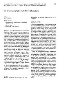
Nonlinear interactions in strained turbulence 108
106
TNL
TNL(t)
t3 104
t2 t1
102
t=0
X(k) 0
10
10 –2
10 –4
kNL(TNL)
kNL(t3)
kNL(t1)
kNL(t2) kdiss
10 – 6 –1 10
0
10
1
2
10
3
10
10
10
4
105
k ˆ iω ˆ i∗ (k) ω
Figure 2. Enstrophy spectrum Ω(k) = showing how the range of k for which RDT is valid (0 < k < kNL (t)) may increase and then decrease as the distortion proceeds. Note at t = 0 the spectrum is undistorted, at t = t1 the distortion is weak (β ∼ 1), and when t = t2 , t3 , TNL it is assumed that the distortion is strong (β � 1). First kNL (t) increases and then decreases, until at t = TNL the r.m.s. vorticity is a maximum; this is also the limit of t for an accurate RDT approximation to r.m.s. velocity. The dashed curve, for kNL (t) shows the limit of the RDT calculation. For k > kNL the spectral curves are not computed; it is assumed (based on experiment) that the spectra revert to their undisturbed form.
Inspection of (2.13a) and (2.13b) shows that only (3.31a) is the relevant form for ˆ g(k; k10 , 0, 0) as β → 0. When k20 = k30 = 0, it follows from its definition that ˆ 1 (k1 , 0, 0) = 0. Since the only terms in (2.13a) and (2.13b) involving ω ˆ 20 and ω ˆ 30 are ω 0 0 multiplied by k2 and k3 , it follows that all the numerators are zero and therefore ˆ g(k; k10 , 0, 0) = 0. Thus, for this limiting case, the magnitude of the nonlinear terms in (2.17) grows faster than that of the largest linear term by a factor β −1 . ˆ (0) (k)β −2 = Q ˆ (0) (k) exp(2τ) and Q ˆ (0) (ω (0) , k, β) = ˆ (0) (ω (0) , k, β) = Q Substituting Q 1 1 1 2 (0) ˆ (k) into the inviscid versions of (3.1a) and (3.1b) and solving we find that to Q 2 first order the solution is ˆ (0) (k), ˆ 1 (k, τ) ∼ ω ˆ 10 (k) exp(τ) + � exp(2τ)Q ω 1 ˆ (0) (k). ˆ 2 (k, τ) ∼ ω ˆ 20 (k) exp(−τ) + �Q ω 2
(3.32a) (3.32b)
A secularity appears in the first-order terms and thus the zeroth-order RDT solution for the energy-containing eddies (k ∼ O(1)) is valid for τ . ln �−1 ,
(3.33)
1 ln �−1 ∼ TNL . S
(3.34)
or, in dimensional terms, t.
348
N. K.-R. Kevlahan and J. C. R. Hunt
This corresponds to the ‘large strain’ criterion as defined by the limit given in (2.10a). Note that since the ratio of the two time limits (3.17) and (3.33) is �−1 � 1, (3.35) ln �−1 it follows that in case (b) RDT for the energy-containing eddies is valid for a much shorter time than in case (a). We now calculate a time limit that takes into account the wavenumber, and we consider the different criteria for the validity of RDT for vorticity and velocity calculations. Using the asymptotic relation (3.31) and keeping only the leading-order terms in ˆ (0) becomes the numerator of (3.2a), we find that the zeroth-order nonlinear term Q 1 Z ∞Z ∞ ˆ (0) (ω ˆ 10 (k − (k10 , 0, k30 ))ω ˆ (0) , k, β) = πβ −2 k2 ˆ 10 (k10 , 0, k30 ) dk10 dk30 . (3.36) ω Q 1 −∞
−∞
Note that the nonlinear term in the stretched direction (the largest nonlinear term) depends on gradients in the compressed direction of enstrophy in the stretched direction. The larger these variations, the larger the nonlinear term. ˆ 10 (k1 , 0, k3 ) 6= 0 in this case, we can use (3.20) to choose the following form Since ω ˆ for ω10 (k): � 0, k 6 1, k > kdiss ˆ 10 (k) = ω (3.37) k1 k −(1+p) , 1 < k < kdiss . ˆ 10 (k) in (3.36), changing to cylindrical coordinates and integrating Substituting for ω over directions we find �Z k−1 � Z kdiss (0) 2 −2 0 −(1+p) 02−p 0 0 −(1+p) 02−p 0 ˆ (k − k ) k dk + (k − k) k dk |Q1 (k, β)| 6 π β k2 1
6
2
k+1 2
2π −2 2−p 2π −2 3−p β k2 k β k , 6 p p
(3.38)
where we have used the fact that |k − (k10 , 0, k30 )| > ||k| − |(k10 , 0, k30 )|| = |k − k 0 |, and ˆ (0) (k, β)| has the same dependence on k as in the have assumed that k � 1. Thus |Q 1 previous case. If we now take the ratio of first- to second-order terms in (3.32a) using (3.37) and (3.38) we find that the range of validity of the RDT approximation is � exp(τ)
2π 2 k2 3 k .1 p k1
or � exp(τ)
2π 2 3 k . 1, p
(3.39)
if we assume that k2 /k3 ∼ 1 for simplicity. Again, the RDT criterion is only weakly dependent on the power law p of the energy spectrum of the inertial range. Using (3.39) we can derive the limits of the RDT approximation in time and in wavenumber: �1/3 � . (3.40a, b) τ . ln �−1 k −3 ∼ τNL (k), k . �−1 exp(−τ) Thus RDT is valid for shorter times at larger wavenumbers, and over a decreasing range of smaller wavenumbers as time increases. In dimensional terms the above expressions become � � �1/3 � 1 1 S S −3 (Lk) exp(−St) ∼ kNL . (3.41a, b) ∼ tNL (k), k . t . ln S u0 /L L u0 /L Following the same procedure as in (3.28), it follows that the amplification of vorticity
Nonlinear interactions in strained turbulence
349
at time t is ω2
NL
(t) ∼ exp( 13 (3 + 2p)St)�−(3−2p)/3
for
3 − 2p > 1.
(3.42a)
Thus RDT overestimates mean square vorticity by a ratio that increases like �(3−2p)/3 exp( 13 (3 − 2p)St). As in the previous case the RDT estimate for mean-square velocity remains accurate until kNL = O(1). We can now estimate the maximum r.m.s. vorticity while the RDT approximation is the dominant effect as ω ∼ 1. (3.42b) S Therefore the turbulence vorticity can reach the magnitude of the applied strain before the RDT approximation fails (i.e. the turbulence vorticity can be amplified to the same magnitude as the applied strain under RDT conditions). ˆ Given this sensitivity to the form of g(k; k0 ) as k20 → 0 it is necessary to establish in which kinds of turbulence the conditions (3.15a) and (3.30a) apply. The condition ˆ1 = ˆ 1 (k1 , 0, k3 ) = 0, and therefore, since ω (3.15a) in the limit β → 0 implies that ω i(k2 uˆ 3 − k3 uˆ 2 ), uˆ 2 (k1 , 0, k3 ) = 0. (3.43a) This is equivalent in physical space to the condition Z ∞Z ∞Z ∞ u2 (x) dx2 exp(i(k1 x1 + k3 x3 )) dx1 dx2 dx3 = 0, (3.43b) −∞
or
−∞
−∞
Z
∞ −∞
u2 (x) dx2 = 0.
(3.43c)
As explained by Batchelor (1953), for a homogeneous random function the integral (3.43c) is not convergent. If turbulence is defined within a box of sides X1 , X2 , X3 , and zero outside it, the integral (3.43c) is now finite but oscillates in time or as X2 varies. Its magnitude is Z ∞ u2 (x) dx2 ∼ u0 L. (3.44a) −∞
Of course this is consistent with the mean of the turbulence being zero, since Z ∞Z ∞Z ∞ 1 L3 u0 u2 = u2 (x) dx = O( ) X1 X2 X3 −∞ −∞ −∞ X1 X2 X3 → 0 as (L3 /X1 X2 X3 ) → 0. Such a situation might arise in practice when the turbulence consists largely of eddies with their longitudinal velocity u1 symmetric about the plane x2 = 0, e.g. a jet entering a contraction. In this case the condition (3.15a) may be satisfied and therefore the ratio of the nonlinear to the linear terms remains of O(�) for all components of the vorticity until St� = O(1). In this situation the inviscid RDT approximation remains valid for a relatively long time. In the presence of viscosity, the viscous terms may become significant over a long time as explained in the next section. However, in most cases of homogeneous turbulence and homogeneous isotropic DNS, the condition (3.31a) is applicable and then, as shown above, the first-order term in � increases until the time when exp(St)� = O(1) and the expansion becomes invalid. Therefore in this and most other distorted flows the RDT approximation is only valid for a relatively short period.
350
N. K.-R. Kevlahan and J. C. R. Hunt 3.3. Viscous range
If the strain ratio is so strong that β can satisfy β � k(�/Re)1/2 , then the convolution integrals in (3.2a), (3.2b) are determined by the viscous exponential term fˆν2 (k0 , k, β). Before examining the validity of RDT in the viscous range it is helpful to determine the conditions under which RDT remains valid until viscosity becomes important. From (3.6), assuming a Kolmogorov range, viscosity is important for wavenumbers k = O(1) when � � �1/2 . (3.45) β = exp(−τ) � Re Substituting τ = TNL ∼ �−1 from (3.17) in the above equation we find that in case (a) the RDT solution remains valid until viscosity becomes important provided that �−1 exp(−2�−1 ) � Re−1 .
(3.46)
Similarly, substituting τ = TNL ∼ ln �−1 from (3.33) we find that in case (b) the condition for significant viscous effects is � � Re−1 .
(3.47)
The inequality (3.46) shows that in case (a) RDT can remain valid for the largest turbulence scales right up until the viscous range for essentially any Reynolds number provided � < 1. On the other hand, in case (b) (3.47) shows that in high-Reynoldsnumber turbulence viscous effects are significant in RDT only if � is extremely small (RDT usually fails before viscosity becomes important). Because the convolution integrals in the k20 - and k30 -directions are of the form Rb I(x) = a f(t) exp(xφ(t)) dt with x � 1 we can use Laplace’s method to calculate their behaviour to leading order: I(x) ∼
(2π)1/2 f(c) exp(xφ(c)) , (−xφ00 (c))1/2
x → +∞
(3.48)
where φ(t) has a maximum at t = c (see Durbin 1979). Using Laplace’s method and assuming that ki > 0 we find that in the far viscous range (�/Re)k 2 β −2 � 1 our generic integral in (3.4) becomes I(k, β) ∼ π
� � � 4Re −2 k2 β(ln β −2 )−1/2 exp (β −2 k22 + ln β −2 k32 ) 4Re Z�
×
∞
−∞
0
ˆ g(k; k10 , 12 k2 , 12 k3 ) exp(−(k12 − k1 k10 )) dk1 ,
(3.49)
and therefore � � ˆ i(0) (k, β)πai (k) 4Re −2 ω �k22 −2 (0) ˆ Qi (k, β) ∼ k exp − β + O(�), ωi0 (k) � 2 4Re
(3.50)
where ai (k) is the integral in (3.49) and we have assumed that β 6 � in the viscous range. Inserting (3.50) into (3.1a), (3.1b) and solving we find that to first order the solution is
Nonlinear interactions in strained turbulence 351 � � � � (0) 2 2 ˆ (k, β)πai (k) 2Re −2 �k �k ω ˆ i (k, β) = ω ˆ i(0) (k, β) exp − 2 β −2 + � i ω k2 exp − 2 β −2 ˆ i0 (k) ω 2Re � 4Re +O(�2 ).
(3.51)
Thus a secularity develops and, if for simplicity we assume that O(1), RDT is only valid while � 2 � �k2 −2 β Re exp < 1, 4Re
ˆ i0 (k) (2πai (k)k2−2 )/ω
∼
(3.52)
but in the viscous range (�/Re)k 2 β −2 � 1 by definition, and therefore RDT fails immediately in the viscous range. However, one notes that in the viscous range both the linear and nonlinear terms are decreasing like exp(− exp(2τ)). Thus, by the time the nonlinear terms overwhelm the linear terms, the vorticity field will have decayed essentially to zero. Combining the fact that RDT fails immediately in the viscous range with the inequalities (3.46) and (3.47), we see that in case (a) RDT remains valid for the largest turbulence scales for � �1/2 ! 1 Re (3.53) ∼ TNL , t . ln S � whereas in case (b), provided the Reynolds number is large, the limit of RDT is usually still given by (3.41).
4. Example calculations 4.1. Numerical calculation of the nonlinear terms In order to check the asymptotic analysis in the previous section we have calculated the nonlinear terms (3.2a) and (3.2b) numerically for velocity fields corresponding to the two initial conditions set out in (3.15) and (3.31a). Following Townsend (1976) we take as a particular form the vorticity field of an ‘eddy’ that is highly localized and whose velocity decreases rapidly away from its centre. In the first case the vorticity ω2 of the eddy is aligned in the compressed direction x2 , and satisfies (3.43c); in the second case the same eddy is aligned with the x1 stretched direction (which does not satisfy (3.43c)). The Fourier transform of the vorticity of the first case of the ‘Townsend’ eddy is defined by ˆ 1 (k) = −k1 k2 exp(− 12 k 2 ), ω ˆ 2 (k) = ω ˆ 3 (k) = ω
(k12
+ k32 ) exp(− 12 k 2 ), −k2 k3 exp(− 12 k 2 ).
(4.1) (4.2) (4.3)
ˆ 1 (k1 , 0, k3 ) = 0, and hence uˆ 2 (k1 , 0, k3 ) = 0. When the eddy is initially Note that ω ˆ 1 is defined similarly by exchanging the indices aligned with the stretched direction, ω 1 and 2 in the above equations. ˆ i (k, t) are shown in figure 3, for the The results of the numerical calculations for ω parameters Re = 102 , � = 10−2 and the particular wavenumber k = (1.5, 0.8, 1.3). Two special NAG subroutines were used to calculate the three-dimensional convolution integrals whose integrals, as our asymptotic analysis demonstrates, are very large over a narrow range of the variables. The first subroutine, DO1GCF, uses a number the-
352
N. K.-R. Kevlahan and J. C. R. Hunt
oretical method and the second subroutine, DO1FCE, uses a seventh-order adaptive grid. These results clearly verify the analytical asymptotic calculations of the previous section: the zeroth-order nonlinear terms remain negligible until the far viscous range if the eddy is aligned in the compressed direction, but the nonlinear terms grow faster than the linear terms by a factor β −1 if the eddy is aligned in the stretched direction. In the far viscous range, where β −1 � (Re/�)1/2 = 100, the nonlinear terms grow faster than the linear ones by a factor exp(�k22 β −2 /(4Re)) as predicted by the asymptotic calculations. Figure 4 shows schematically how ‘Townsend eddies’ respond differently to irrotational strain depending on their orientation. Because the Townsend eddy is in fact made up of concentric vortex rings we consider the response of single vortex rings in the two planes perpendicular to the straining motion, which is easier to understand. In figure 4(b) where the ring is compressed so that the vorticity field reduces to ω3 (x2 ) and the velocity field of the ring reduces to u1 (x2 ), the nonlinear terms are identically zero. In figure 4(c) the ring is in the (x1 ,x3 )-plane and is stretched so that it becomes elliptical, and its cross-section is also distorted so that it becomes flatter. Neither state is steady: the nonlinear terms are significant. The ring itself bends because the induced velocities u2 are larger at the curved ends; and each end of the cross-section rotates faster than the centre thus rolling it up and eventually diffusing the vorticity across a thicker vortex core or producing a concentric sheet structure as discussed in §4.2. Marshall & Grant (1994) have calculated numerically and analytically the response of ‘thin’ vortex rings to irrotational straining. They have also found that stretching can inhibit the destabilizing nonlinear terms and allow the linear theory to remain valid for an extremely long time (sometimes until the aspect ratio of the stretched vortex is only 0.008!). 4.2. Self-induced distortion of a vortex ring Figure 4(c)(iv) shows how the cross-section of a vortex ring becomes elongated into a strip of length 2L, width 2l, and thickness 2h by irrotational strain. The length of the vortex ring increases with time and the thickness decreases with time, while the width remains constant. A simple Biot-Savart calculation (e.g. Batchelor 1967) shows that Z Z Z ω1 l h L x3 − x03 (4.4a) dx0 dx0 dx0 u2 (x3 ) = − 02 02 4π −l −h −L (x1 + x2 + (x3 − x03 )2 )3/2 1 2 3 � � ω1 h x3 − l ln , (4.4b) u2 (x3 ) ≈ π x3 + l where we have assumed that L � ||x3 | − l| and h � ||x3 | − l|. Thus, � � ω1 h 2l |u2 (x3 )| ∼ ± ln at x3 = ∓l. π h
(4.4c)
Since |∂u2 /∂x3 | is maximum at each end of the strip the two ends roll up, which can be described by the change of the tangent angle (see figure 4c(v)). From (4.4b) ∂u2 ω1 h 2l dθ(x3 ) ≈ ≈ , dt ∂x3 π x23 − l 2
(4.5)
353
Nonlinear interactions in strained turbulence 102
100
100
10 –2
10 –2
10 –4
10 –4
10 –6
10 –6
10 –8
10 –8 10 –10 0 10
(a) 101
102
10 –10 10 –12 103 100
104
100
102
10 –2
100
10 –4
10 –2
10 –6
10 –4
10 –8
10 –6 10 –8 0 10
(c) 101
102
(b) 101
102
10 –10 10 –12 103 100
c
103
(d) 101
102
103
c
Figure 3. Numerical calculation of the growth of linear and zeroth-order nonlinear terms when ˆ (0) (t)|; – – – – –, |ω ˆ i(0) (t)|; a Townsend eddy is distorted by plane irrotational straining where —, |Q i (0) ˆ i (t)| and strainR ratio c = exp(t) = β −1 . Notice that when the eddy is aligned in — · —, |�/Reχ2 (t)ω ∞ the compressed direction (so that −∞ u2 (x) dx2 = 0) the nonlinear terms increase only at the same rate as the linear terms. When the eddy is aligned in the stretched direction however, the nonlinear terms increase at a rate c times faster than the linear terms. (a) Eddy axis in the compressed ˆ 1 equations. (b) Eddy axis in the compressed direction x2 , ω ˆ 2 equations. (c) Eddy axis direction x2 , ω ˆ 1 equations. (d ) Eddy axis in the stretched direction x1 , ω ˆ 2 equations. in the stretched direction x1 , ω
but ω1 (t) ∼ ω10 exp(St). Hence at l − |x3 | ∼ h, ω1 ω10 dθ ∼ ∼ exp(St). dt π π
(4.6)
When dθ/dt ∼ S, the self-induced rolling up motion is more significant than the applied straining. This occurs at a time τmax such that ω10 exp(Sτmax ). (4.7) S∼ π
354
N. K.-R. Kevlahan and J. C. R. Hunt
Hence,
1 �π� ln , (4.8) S � where � = ω10 /S � 1. Based on this criterion the maximum value of ω1 , ω1max , is significantly greater than S since τmax ∼
ω1max ∼ ω10 exp(Sτmax ) = πS.
(4.9)
It also implies that h reaches an asymptotic thickness � (4.10) hmin ∼ l exp(−Sτmax ) ∼ l . π If the Reynolds number is large enough the self-induced accelerating motion may inhibit the diffusion of vorticity and then the strip may continue rolling up to form a spiral vortex sheet structure.
5. Application of RDT analysis to the structure of homogeneous turbulence 5.1. Vorticity alignment Probability distribution functions (PDFs) of DNS turbulence show that the vorticity vector aligns preferentially with the intermediate eigenvector of strain (e.g. Ashurst et al. 1987; Vincent & Meneguzzi 1991). Vincent & Meneguzzi (1994) investigated the development over time of turbulence structure in DNS when the initial condition is a random Gaussian velocity field in which the vorticity is very small and structureless. As the nonlinear processes develop, the first vortical structures to appear are pancakelike regions in which the vortex lines lie in sheets of finite width. Since this distribution is not stable the sheets bend and roll up to form the first vortex tubes (cf. §4.2). Typically their length is 10 times their diameter, which indicates they are being strained. An important observation is that the vorticity ω is greatly amplified in the sheet phase and that it is aligned with the largest positive eigenvector of the tensor of the large-scale strain Sij (i.e. large on the scale of the tube or sheet). This is to be expected. However, Vincent & Meneguzzi (1994) also find that the vorticity aligns with the intermediate strain eigenvector of the the sheets and they note that the PDF over the entire turbulent flow shows that this alignment develops during the sheet phase. Thus they conclude that the alignment of vorticity with the intermediate strain eigenvector is due to the formation of sheets of intense vorticity. These sheets then roll up to form tubes and these tubes retain the alignment of the sheets. Vortex sheets or layers have been observed in many other DNS with a variety of initial conditions and Reynolds numbers (e.g. Kerr 1987; Ruetsch & Maxey 1992), and the transition from blobs to sheets to tubes has also been carefully investigated using a different DNS code by Ruetsch & Maxey (1992). Furthermore, clear evidence of layered vortex sheets has been found in experimental fully developed turbulence by Schwartz (1990). He observes that the vortex sheets often form tube-like structures which are consistent with the structure of a spiral vortex tube. Thus vortex sheets are a characteristic structure of both DNS and experimental turbulence. This alignment had been predicted by Vieillefosse (1982) and explained kinematically by Jim´enez (1992). Vieillefosse (1982) proposed that a tube is created along the axis of the largest strain, but very soon aligns with the intermediate strain. Jim´enez (1992) showed that a vortex tube has the observed alignment, but did not consider how the tube may have formed. Thus both these explanations suggest that the
355
Nonlinear interactions in strained turbulence (a)
x2 x1 x3
(b) x1
x2
x2 x2
x2
x1 x1
u2
x3
(i) t = 0
x3
(ii)
(iii)
x1
(c) x2
x1
x2
x2
t < TNL
u2 x3
(iii)
x3
t=0 (i)
2l
t > TNL
(ii) 2h (iv) θ (v)
Figure 4. Distortion of vortex rings to show the effect of orientation relative to mean strain. Note that a Townsend eddy consists of many vortex rings with the same axis. Double arrows indicate vorticity direction and single arrows indicate velocity direction. Note that the nonlinear terms are identically zero for a circular vortex ring. (a) Orientation of mean irrotational strain. (b) Vortex ring aligned with the axis in the stretched direction. (i) Initial state. (ii) Initial velocity profile, note R∞ that −∞ u2 (x) dx2 = 0. (iii) Effect of strain, the eddy does not quickly become unstable. (c) Vortex ring aligned with the axis in the compressed direction. (i) Initial state. (ii) Distortion just before nonlinear terms become significant. (iii) The nonlinear terms cause the elliptical vortex ring to deform. (iv) The elliptical cross-section of the vortex ring also deforms, rolling up.
alignment arises only after tubes have formed. However, Vincent & Meneguzzi (1994) specifically considered the explanation of Vieillefosse and rejected it since: “The alignment of vorticity with the intermediate strain eigenvector is found to exist before the shear instability develops, and is the result of vorticity sheet production by strong strain. It is not a consequence of tube formation.” Thus the explanations of Vieillefosse (1982) and Jim´enez (1992) are clearly not sufficient to explain the origin of the observed alignment. Shtilman et al. (1993) have also shown that this alignment cannot be present in random-phase Gaussian flows with the same spectrum as a truly turbulent flow.
356
N. K.-R. Kevlahan and J. C. R. Hunt
We now show that this alignment can be produced by irrotational straining of an initially random flow and in the following subsection we will show that this straining tends to produce vortex sheets rather than tubes. Since the small-scale vorticity ω in these regions of larger-scale strain Sij is initially weak (i.e. |ω| � S), an RDT analysis is valid. The results of §§2 and 3 are now used to analyse the relation between ω and the eigenvectors of sij in a strain given by (2.11) (note that adding viscosity would not affect alignments). Consider the solution for ω and u (given by (2.19), (2.18), (2.5)) at large strain ratio c = β −1 = exp t. From the definition sij = 12 (∂ui /∂xj + ∂uj /∂xi ), the Fourier transform of the small-scale rate-of-strain tensor is � � k1 k1 k3 1 1 2 ˆ ˆ ˆ ˆ ω30 β ω ω30 − ω10 β 2 30 2 k2 k2 k2 k 3 1 1 −1 , ˆ ˆ 10 ˆ 10 β ω ω −2ω (5.1) sˆ ∼ 2 30 k2 � � 1 k3 k1 k3 ˆ 30 − ω ˆ 10 β − 12 ω ˆ 10 β −1 ˆ 10 ω − ω 2 k2 k2 k2 where the subscript 0 indicates initial value of a vorticity component and we have retained only the largest term in each of the components of sˆij . The characteristic equation for the eigenvalues ξi of sˆij is ξ 3 − P ξ + Q = 0.
(5.2)
At large times the large and small roots of (5.2) are proportional to β −1 . The roots of a cubic equation with three distinct real roots must satisfy ξ1 ξ2 ξ3 = Q, hence the intermediate eigenvalue ξ2 must decay exponentially with time: ξ2 ∝ β 2 = exp(−2t).
(5.3)
(Note that the fact that the magnitude of the intermediate eigenvalue decreases rapidly while the magnitude of the other eigenvalues increases rapidly may help explain why the average value of the intermediate eigenvalue measured in DNS is significantly smaller than the other two, typical values are 3:1:−4, e.g. Kerr 1987.) Thus at large times the eigenvalues of sij approach asymptotically ξ1 = 12 ω10 β −1 , ξ2 = 0, ξ3 = − 12 ω10 β −1 ,
(5.4)
with corresponding ‘large positive’ ξ1 , ‘intermediate’ ξ2 and ‘large negative’ ξ3 eigenvectors (0,1,1), (1,0,0), (0,1,−1) respectively. The results (5.3), (5.4) show that the ‘intermediate’ eigenvector of the small-scale motion (ξ2 ) tends to align on a time scale of S −1 with the large positive eigenvector of Sij . From the basic vorticity equation (2.7), when nonlinear and viscous terms are small the small-scale vorticity ω, whatever its initial orientation, aligns with the large positive eigenvector of Sij , on a time scale of S −1 . Therefore the small-scale vorticity ω aligns with the intermediate eigenvector of sij . As the magnitude of the small-scale strain rate ||sij || increases exponentially with time (5.1) it becomes of the order of S = ||Sij || on a time scale t = 1/S ln(�−1 ). This time is much less than the RDT limit TNL ∼ L/u0 (from (3.18)) in case (a), but is equal to TNL (see (3.34)) for case (b). Thus turbulence strain can be amplified by purely linear effects to a value at least as large (and possibly much larger) than the applied strain. However, for TD � TNL the linear relationships between the alignments of vorticity and strain breaks down. Thus for a certain period TD ∼ TNL , the overall
Nonlinear interactions in strained turbulence
357
alignment of the strain (i.e. small and large scale) is dominated by that of the strained vorticity and therefore we conclude that on this time scale the vorticity ω aligns with the intermediate eigenvector of the total rate of strain. This is what is observed in the numerical experiments. The enhancement of alignment by irrotational straining has recently been demonstrated in compressible turbulence, when it passes through a shock front (Kevlahan, Krishnan & Lee 1992). We now calculate the enstrophy production and demonstrate that the structure produced by the irrotational straining is a sheet rather than a tube. 5.2. Enstrophy production After persistent inviscid irrotational straining the RDT solutions ω become (in the reference frame of the eigenvectors of s) (5.5) ω10 = ω1 = ω10 β −1 , 1 1 (5.6) ω20 = √ (ω3 + ω2 ) = √ (ω30 + ω20 β), 2 2 1 1 (5.7) ω30 = √ (ω3 − ω2 ) = √ (ω30 − ω20 β), 2 2 and from equation (5.1) the small-scale rate-of-strain tensor has non-zero components s11 = ξ2 β 2 , s22 = − 12 ω10 β −1 − 12 ξ2 β 2 , s33 = 12 ω10 β −1 − 12 ξ2 β 2 where ξ2 (k)β 2 is the intermediate eigenvalue of s). The enstrophy equation is � �2 D( 12 ω 2 ) ∂ωi = ωi ωj (Sij + sij ) − ν , (5.8) Dt ∂xj and therefore the contribution to enstrophy production from the small-scale rate of strain is given by 2 −2 β ξ2 β 2 ωi ωj sij = ω10 2 2 2 − 14 (ω20 β + 2ω20 ω30 β + ω30 )(ω10 β −1 + ξ2 β 2 ) 2 2 2 + 14 (ω20 β − 2ω20 ω30 β + ω30 )(ω10 β −1 − ξ2 β 2 ),
(5.9)
which for long times becomes 2 2 − 12 ξ2 ω30 − ω10 ω20 ω30 . ωi ωj sij ∼ ξ2 ω10
(5.10)
2 2 However, because of isotropy hω10 i = hω20 i = 13 hω02 i and hω10 ω20 ω30 i = 0 and hence
GNL = hωi ωj sij i = 16 hξ2 ω02 i,
(5.11)
which may be either positive or negative depending on the sign of ξ2 . The contribution to nonlinear enstrophy production from the applied strain is easily found from (5.8) and (5.6) to be 2 iβ −2 S, GL = hωi ωj Sij i = hω10
(5.12)
which is always positive. Note that equations (5.1) and (5.7) also show that the vorticity aligns with the vortex stretching vector of the applied strain ωj Sij . This alignment has also been observed in DNS (Shtilman et al. 1993). Equation (5.11) shows that enstrophy is created (destroyed) by small-scale interactions if ξ2 > 0 (ξ2 < 0). A related kinematical result was proved by Betchov (1956).
358
N. K.-R. Kevlahan and J. C. R. Hunt
Of course, only a dynamical analysis can indicate the conditions under which this relation actually occurs. As we discovered in §3, the enstrophy generated by small-scale interactions is negligible compared with the enstrophy generated by the applied strain as long as the applied strain S is significant. However, in a turbulent flow small-scale turbulence can be rapidly advected through any given region of irrotational straining. Once the small-scale turbulence leaves the straining region the major contribution to enstrophy generation is given by equation (5.11), and then whether enstrophy is created or destroyed depends on the sign of ξ2 . Although we found in §3 that in general (case b) the largest nonlinear terms grow faster (by O(β −1 )) than the linear terms, this does not mean that the nonlinear enstrophy growth is faster than the linear enstrophy growth. In fact, as we have seen above, to leading order GNL is a constant while GL increases in time like β −2 . ˆ1 This is because the fastest growing nonlinear terms are the advection terms of Q which do not produce enstrophy. Thus RDT estimates of enstrophy production (at wavenumbers where RDT is valid) should be accurate. The destruction of enstrophy by the small-scale strain part of (5.8) in some strained regions and its production in other strained regions (depending on local values of the eigenvalues of s) would eventually produce an intermittent vorticity distribution. Thus, in a turbulent flow where the vorticity is initially evenly distributed, irrotational straining tends to concentrate vorticity into small regions – vortex sheets. Therefore we have seen that irrotational straining is able to produce both the alignment seen in the DNS of Vincent & Meneguzzi (1994) and the vortex sheets observed in the experiments of Schwartz (1990). A recent perturbation analysis and three-dimensional numerical simulation by Passot et al. (1995) has shown that when a strained vortex sheet becomes unstable, vorticity concentrates into steady (possibly spiral) tubular structures with finite amplitude. They conclude that this is the process that creates the intense and long-lived vortex tubes observed in DNS and experiments (Douady, Couder & Brachet 1991) of homogeneous turbulence. Hence one could expect large-scale irrotational straining to produce an intermittent distribution of spiral vortex tubes. The experimental observations of Schwarz (1990) indicate that at high Reynolds numbers the tubes retain a structure composed of rolled up vortex sheets, and thus should retain the alignment developed during the sheet phase. The analyses presented in §§5.1 and 5.2 are valid over a finite time TNL (which, estimated by (3.18), is somewhat greater than S −1 ) before the nonlinear effects become significant. A deeper understanding of this surprising result will require a more detailed analysis to show how persistent irrotational strain on a time scale much greater than S −1 affects alignment of ω and ξ 2 . Another feature of turbulent flow is the presence of variations of large-scale strains acting in adjacent parts of the flow. There may be a good reason for neglecting the effects of adjacent strain because of the ‘sheltering’ effect of vorticity, which can isolate different regions of irrotational strain (Hunt et al. 1997).
6. Discussion The main result of this paper has been to demonstrate quantitatively the sensitivity to initial and boundary conditions of turbulence undergoing plane irrotational strain. In particular, we considered the validity of the rapid distortion theory (RDT) approximation, which applies initially if (u0 /L)/S = � � 1, where u0 is the initial r.m.s. velocity of the turbulence, L is the initial integral scale of the turbulence and S is the
Nonlinear interactions in strained turbulence
359
2.5
2.0
1.5
q2 q20 1.0
0.5
0 1
2
3
4
c Figure 5. Comparison between inviscid RDT (lines) and data from a contracting wind-tunnel experiment (circles) for the change in turbulent kinetic energy q 2 due to plane irrotational straining of turbulent flow (data from Tucker & Reynolds 1968). The initial condition is roughly � = 2.8. The RDT results have been corrected to compensate for the natural decay of the turbulence using the model equation q 2 /q02 = (1 + 2ε0 /(nq02 S) ln c)−n where ε0 is the initial dissipation rate, q0 is the initial turbulent kinetic energy and n is a parameter which was found to be 1.24 in the absence of the distortion.
applied strain rate. The RDT solution is the leading-order term in the perturbation series solution in terms of �. We used the asymptotic form of the convolution integrals for the zeroth-order nonlinear terms when the strain ratio β −1 = c = exp(St) � 1 to determine when (in scale and time) the perturbation series in � fails, and hence to estimate the domain of validity of inviscid RDT. The technique introduced here may well be applicable to other distorted flows, with equally interesting results. If the Fourier component of the velocity in the compressed direction uˆ 2 (k) at k2 = 0 is initially zero, i.e. Z ∞ uˆ 2 (k2 = 0) = 0 or u2 (x) dx2 = 0, (6.1) −∞
then the inviscid RDT approximation for the effect of plane irrotational strain on this flow remains valid over a time TNL ∼ L/u0 = TL . This condition describes certain eddy structures in a contracting wind tunnel (see figure 1). However, in most homogeneous isotropic DNS (6.1) is generally not satisfied and the time scale for the validity of RDT is shorter, TNL ∼ 1/S ln(�−1 ). Note that the r.m.s. velocity can be well approximated by linear RDT, even when the r.m.s. vorticity is strongly affected by nonlinear effects. This difference comes from the fact that the slope of the energy spectrum is negative, while the slope of the enstrophy spectrum is positive. Thus r.m.s. vorticity is sensitive to errors at the small scales where RDT fails first, while r.m.s. velocity is insensitive to these errors. Viscosity dominates in the linear terms when t � (1/S) ln(k−1 (Re/�)1/2 ), and RDT fails immediately in this range. One should note, however, that in this range both the zeroth-order RDT terms and first-order terms have decreased essentially to zero. If (6.1) is satisfied RDT remains valid for the largest scales until the viscous range,
360
N. K.-R. Kevlahan and J. C. R. Hunt 2.5
2.0
1.5
q2 q20 1.0
0.5
0 1
2
3
4
c Figure 6. Comparison between inviscid RDT (lines) and DNS results (circles) for the change in turbulent kinetic energy q 2 due to plane irrotational straining of turbulent flow (data from Lee & Reynolds 1985). The RDT results have been corrected to compensate for the natural decay of the turbulence as in figure 5 and n was found to be roughly 1.5. The dashed curve is the uncompensated RDT prediction. From bottom to top the runs are for initial conditions, � = 2.0, 1.0, 0.5, 0.25, 0.125, 0.0260, 0.0065. The asymptotic analysis gives the period of validity of RDT as c = n.a., n.a., n.a., 4.0, 8.0, 38.5, 77.5 respectively (where n.a. = not applicable).
and thus in this case the effective time limit for RDT for the largest turbulence scales is TNL ∼ (1/S) ln((Re/�)1/2 ). If (6.1) is not satisfied then RDT usually fails before reaching the viscous range and the inviscid estimate for the validity of RDT remains valid. If (6.1) holds, then the maximum amplification of vorticity under RDT is ω1 /S ∼ � exp(�−1 ) � 1, otherwise the maximum amplification of vorticity under RDT is ω1 /S ∼ 1. This result is interesting because it shows that in all flows turbulence vorticity can be amplified to the magnitude of the applied strain while linear RDT is approximately valid, but that in some flows, with certain eddy structures and if strain is large enough, RDT remains valid even when the turbulence vorticity has become much larger than the applied strain. We find that the order-of-magnitude estimate for the time period of the validity of RDT based on the criterion (2.10b), namely that u0 (t)/L � max(S, 1/t), is an underestimate since u0 (t)/L increases exponentially in time. Expressed in similar terms, we find instead that u0 /L � 1/t if (6.1) is satisfied, and u0 /L � S/ exp(St) otherwise, where u0 = u0 (t = 0). Interestingly, the ‘crudest’ order-of-magnitude estimate, u0 /L � 1/t, is only accurate in the specific case (6.1). The results on the validity of RDT for the inviscid and viscous ranges may be combined and summarized concisely in terms of the strain ratio c = exp(St) as �1/2 � SRe , symmetric in compressed direction, (6.2a) c< u0 /L � �1/2 ! SRe S , , in general, (6.2b) c < min u0 /L u0 /L where we have considered the largest turbulent length scales.
Nonlinear interactions in strained turbulence
361
Another interesting result is that the fastest growing nonlinear terms are the advection terms in the equation for ω1 (the exponentially increasing vorticity in the stretched direction). If the advection terms are neglected the RDT solution for ω1 is valid for all time up to first order. The RDT solution for ω2 fails earlier, but ω2 decreases exponentially in time. Thus, the generation of enstrophy (which does not depend on advection) should be very accurately predicted by RDT. Several experiments (MacPhail 1944; Townsend 1954; Mar´echal 1967; Tucker & Reynolds 1968; Reynolds & Tucker 1975) have been carried out to investigate the effect of irrotational distortion on turbulence. All these experiments used a wind-tunnel set-up similar to that shown schematically in figure 1. The experiments attempted to verify RDT, but unfortunately the ratio (u0 /L)/S = �, which should be very small for RDT to be initially valid, was at best approximately 2.8! On the other hand, by extending the contracting section of the wind-tunnel Mar´echal was able to obtain strain ratios as high as 14. Because � 6� 1 in these experiments the analysis of the period of validity of RDT derived here is not formally applicable. However figure 5 shows that the RDT prediction of the evolution of turbulent kinetic energy is still remarkably accurate at least until c = 4. As explained in §3.2, RDT should be particularly good at predicting the evolution of turbulent kinetic energy (or, equivalently, r.m.s. velocity) . In addition, as pointed out by Reynolds & Tucker (1975): “the rapid-distortion hypothesis already accounts for most features of the response.” The only DNS of the effect of plane irrotational strain on turbulence is the study of Lee & Reynolds (1985). These simulations were able to produce very high strain rates (� � 1), but at a relatively low Reynolds number (Rel ∼ 50) and only until a moderate strain ratio (c 6 4). The results of these simulations are shown in figure 6 along with RDT predictions corrected for the decay of the turbulence. The agreement with RDT is reasonable for all the simulations (even those with � 6� 1) and is consistent with the period of validity of RDT calculated here. It is important to note, however, that the curve for the smallest � represents only 4 time steps and thus it is unlikely that any nonlinear change in the turbulence could have developed. To properly verify the validity calculations it would be necessary to go to much higher strain ratios. Again, perhaps the most surprising result is that RDT works very well even when the nonlinear and linear terms are initially of the same order (� ∼ 1), and remains valid up to moderate strain ratios. The surprising accuracy of RDT even when � ∼ 1 may be due to the fact that, as shown by the asymptotic analysis, the straining motion modifies the turbulence so that the nonlinear terms are inhibited. This explanation is supported by the fact that �(t) actually decreases during the distortions for the weaker strain DNS: from (2.0, 1.0, 0.5, 0.25) to (0.38, 0.33, 0.27, 0.21). The inhibition of the nonlinear terms thus appears strongest when the applied strain is weak! Thus, even if the nonlinear terms are initially of the same order as the linear terms RDT may still be a good approximation. The mathematical results presented here are also quite consistent with the experimental results for small-scale turbulence undergoing very strong large-scale distortion around a circular cylinder of radius a obtained by Britter, Hunt & Mumford (1979). R In this experiment S dt ≈ 1.2, β ≈ 0.3, and � ≈ 0.1 for the small-scale turbulence case. The experimental results on the centreline showed that the RDT results were approximately correct for the amplified velocity components (u2 , u3 ) (in the notation of this paper), but that RDT was only accurate near the beginning of the distortion
362
N. K.-R. Kevlahan and J. C. R. Hunt
(where the radius r > 1.5) for the components that are predicted to decrease (u1 ) . At larger strains u1 increases which shows that nonlinear effects have a greater impact on the velocity components that are diminished (i.e. in the stretched direction) than on those that are amplified (i.e. in the compressed and normal directions). Generalizing the criterion (3.34) to a variable strain leads to Z TNL S dt ∼ ln(�−1 ). (6.3) 0
Taking the potential flow around the cylinder, U(r) = U0 (1 − a2 /r2 ), as the applied strain we find from (6.3) that the value of r = rNL for the radius along the stagnation line at which the nonlinear terms become significant is rNL ≈ 1.1. (6.4) a The nonlinear effects tending to reduce the anisotropy were observed to become significant at r/a ≈ 1.3, i.e. slightly sooner than the time estimated by (6.4). The spectra of u2 and u3 on the stagnation line show that when r/a = 1.2, or β = 0.1, the amplification predicted by RDT is observed to be reduced when k1 > 1; this can be compared to the prediction of (3.41b) that � �1/3 0.3 kNL L ∼ ≈ 1.4. (6.5) 0.1 These estimates are not formally applicable to the problem of turbulent flow around a cylinder (because the strain is non-uniform and there is also a blocking effect), but they nevertheless give reasonable estimates of the range of validity of RDT. Around the sides of the cylinder on the centreline θ = π/2 where the strain (S) is smaller and the time of distortion is large, however, the agreement with RDT is not as good. Perhaps the most general point to emerge is that a weak random vorticity field can be amplified by a larger-scale strain so that its strain rate becomes of the same order as the applied strain. This is because the nonlinear processes, which might have inhibited this growth, are themselves inhibited by the straining. In other words strained turbulence adjusts itself so as to reduce to a consistent extent the ‘scrambling’ effects on its own amplified vorticity. This helps explain why weak turbulence can be so strongly amplified at the stagnation point of cylinders (Sadeh & Brauer 1980). At a more general level, this ‘adjustment’ plausibly explains an essential feature of the cascade process of turbulence: that small-scale eddy motions have higher strain rates than those of the large-scale motions that provide their energy. We are grateful for many conversations with Henrik Rasmussen and other colleagues, especially those at Cambridge, Houston and the Center for Turbulence Research (Stanford and NASA Ames). N.K.-R.K. was supported at DAMTP, University of Cambridge by an Overseas Research Scholarship and by British Gas, and ´ later at LMD, Ecole Normale Sup´erieure by grant ERBFMBICT950365 of the European Community programme for the Training and Mobility of Researchers. This paper is based on the presentation at W. C. Reynolds’s 60th birthday in 1993.
Nonlinear interactions in strained turbulence
363
REFERENCES Ashurst, W. T., Kerstein, A. R., Kerr, R. M. & Gibson, C. H. 1987 Alignment of vorticity and scalar gradients with strain rate in simulated Navier–Stokes turbulence. Phys. Fluids 30, 2343–2353. Batchelor, G. K. 1953 Homogeneous Turbulence. Cambridge University Press. Batchelor, G. K. 1967 An Introduction to Fluid Dynamics. Cambridge University Press. Batchelor, G. K. & Proudman, I. 1954 The effect of rapid distortion of a fluid in turbulent motion. Q. J. Mech. Appl. Maths 7, 83–103. Betchov, R. 1956 An inequality concerning the production of vorticity in isotropic turbulence. J. Fluid Mech. 1, 497–504. Blackburn, H. M., Mansour, N. N., & Cantwell, B. J. 1996 Topology of fine-scale motion in turbulent channel flow. J. Fluid Mech. 310, 269–292. Britter, R. E., Hunt, J. C. R. & Mumford, J. C. 1979 The distortion of turbulence by a circular cylinder. J. Fluid Mech. 92, 269–301. Cambon, C. 1982 Etude spectrale d’un champ turbulent incompressible, soumis a des effets couples de deformation et de rotation, imposes exterieurement. PhD thesis, L’Universit´e Claude Bernard, Lyon. Cambon, C., Benoit, J.-P., Shao, L. & Jacquin, L. 1994 Stability analysis and large–eddy simulation of rotating turbulence with organized eddies. J. Fluid Mech. 278, 175–200. Cambon, C. & Jacquin, L. 1989 Spectral approach to non-isotropic turbulence subjected to rotation. J. Fluid Mech. 202, 295–317. Cambon, C., Mansour, N. N. & Godeferd, F. S. 1997 Energy transfer in rotating turbulence. J. Fluid Mech. 337, 303–332. Craik, A. D. D. & Criminale, W. O. 1986 Evolution of wavelike disturbances in shear flows: a class of exact solutions of the Navier–Stokes equations. Proc. R. Soc. Lond. A 406, 13–26. Douady, S. Couder, Y. & Brachet, M. 1991 Direct observation of the intermittency of intense vorticity filaments in turbulence. Phys. Rev. Lett. 67, 983–986. Durbin, P. A. 1979 Asymptotic expansion of Laplace transforms about the origin using generalised functions. J. IMA 23, 181–192. Fraenkel, L. E. 1969 On the method of matched asymptotic expansions, Parts I, II and III. Proc. Camb. Phil. Soc. 65, 209–284. Fung, J. C. H., Hunt, J. C. R., Malik, N. A. & Perkins, R. J. 1992 Kinematic simulation of homogeneous turbulent flows generated by unsteady random Fourier modes. J. Fluid Mech. 236, 281–318. Gence, J. N. & Mathieu, J. 1980 The return to isotropy of an homogeneous turbulence having submitted to two successive plane strains. J. Fluid Mech. 101, 555–566. Hunt, J. C. R. 1973 A theory of turbulent flow round two-dimensional bluff bodies. J. Fluid Mech. 61, 625–706. Hunt, J. C. R. & Carruthers, D. J. 1990 Rapid distortion theory and the ‘problems’ of turbulence. J. Fluid Mech. 212, 497–532. Hunt, J. C. R., Durbin, P. A., Kevlahan, N. & Fernando, J. S. 1997 Sheltering effects of vorticity and vortex sheets. (In preparation). Hunt, J. C. R. & Kevlahan, N. K.-R. 1994 Rapid distortion theory and the structure of turbulence. In Proc. Monte Verit´ a Colloquium on Turbulence (ed. T. Dracos & A. Tsinober), pp. 1–18. Birkhauser. Jime´ nez, J. 1992 Kinematic alignment effects in turbulent flows. Phys. Fluids A 4, 652–654. Kerr, R. M. 1987 Histograms of the helicity and strain in numerical turbulence. Phys. Rev. Lett. 59, 783–786. Kevlahan, N. Krishnan, M., Lee, S. 1992 Evolution of the shock front and turbulence structures in the shock/turbulence interaction. In Studying Turbulence using Numerical Simulation Databases - IV, Proc. 1992 Summer Program. CTR. Kida, S. & Hunt, J. C. R. 1989 Interaction between different scales of turbulence over short times. J. Fluid Mech. 201, 411–445. Launder, B. E. 1989 Second moment closure: present and future. Intl J. Heat Fluid Flow 10, 282–299.
364
N. K.-R. Kevlahan and J. C. R. Hunt
Lee, M. J. & Reynolds, W. C. 1985 Numerical experiments on the structure of homogeneous turbulence. Rep. TF-24. Department of Mechanical Engineering, Stanford University. McComb, W. D. 1990 Physics of Turbulence. Clarendon Press. MacPhail, D. C. 1944 Turbulence changes in contracting and distorting passages. R. Aircraft Establishment Aero Rep. 1928. Mare´ chal, J. 1967 Anisotropie d’une turbulence de grille d´eform´e par un champ de vitesse moyenne homog`ene. C. R. Acad. Sci. Paris 265 A, 478–479. Marshall, J. S. & Grant, J. R. 1994 Evolution and breakup of vortex rings in straining and shearing flows. J. Fluid Mech. 273, 285–312. Passot, T., Politano, H., Sulem, P. L. & Angilella, J. R. 1995 Instability of strained vortex layers and vortex tube formation in homogeneous turbulence. J. Fluid Mech. 282, 313–338. Reynolds, A.J. & Tucker, H.J. 1975 The distortion of turbulence by general uniform irrotational strain. J. Fluid Mech. 68, 673–693. Ruetsch, G. R. & Maxey, M. R. 1992 The evolution of small-scale isotropic structures in homogeneous isotropic turbulence. Phys. Fluids A 4, 2747–2759 Sadeh, W. Z. & Brauer, H. J. 1980 A visual investigation of turbulence in the stagnation flow about a circular cylinder. J. Fluid Mech. 99, 53–64. Schwartz, K. W. 1990 Evidence for organized small-scale structure in fully developed turbulence. Phys. Rev. Lett. 64, 415–418. Shtilman, L. Spector, M. & Tsinober, A. 1993 On some kinematic versus dynamic properties of homogeneous turbulence. J. Fluid Mech. 247, 65–77. Townsend, A. A. 1954 The uniform distortion of homogeneous turbulence. Q. J. Mech. Appl. Maths 7, 104–127. Townsend, A. A. 1976 The Structure of Turbulent Shear Flow. Cambridge University Press. Tucker, H. J. & Reynolds, A. J. 1968 The distortion of turbulence by irrotational plane strain. J. Fluid Mech. 32, 657–673. Vieillefosse, P. 1982 Local interaction between vorticity and shear in a perfect incompressible fluid. J. Phys. Paris 43, 837–842. Vincent, A. & Meneguzzi, M. 1991 The spatial structure and statistical properties of homogeneous turbulence. J. Fluid Mech. 225, 1–20. Vincent, A. & Meneguzzi, M. 1994 The dynamics of vorticity tubes in homogeneous turbulence. J. Fluid Mech. 258, 245–254.