2010 International Conference on Biology, Environment and Chemistry IPCBEE vol.1 (2011) © (2011) IACSIT Press, Singapore
Nonlinear Model-Based Control of Non-Ideally Mixed Fermentation Processes
Emily Liew Wan Teng
Yudi Samyudia
Department of Chemical Engineering, Curtin University of Technology, Sarawak, Malaysia.
[email protected]
Department of Chemical Engineering, Curtin University of Technology, Sarawak, Malaysia.
[email protected]
controllers are very unlikely due to its over simplicity which could result inaccuracy of simulation results. Thus, the aim of the present work is to explore different mathematical models for control design. In particular, our focus is to capture the mixing mechanism within a bioreactor so that its effect on the bioreactor’s performance, i.e. yield and productivity can be studied. By analyzing the dynamic behavior of the non-ideally mixed fermentation process, two manipulated variables were used, i.e. aeration rate (AR) and stirrer speed (SS). Using these manipulated variables, a nonlinear model-based controller is designed, where two different models are implemented in the controller design. The paper is organized as follows. Firstly, the process modeling is described and physical parameters are determined by validating the model with experiment data. Next, nonlinear control strategies are developed. The effectiveness of the nonlinear controller is evaluated via simulation, where different disturbance scenarios are explored. The results of the different control strategies are discussed. Finally, conclusions end the paper.
Abstract—In this paper, we consider a non-ideally mixed fermentation process, which exhibits a challenging dynamics for control design. Due to the non-ideal mixing condition in the bioreactor, new control strategies by using aeration rate and stirrer speed as manipulated variables are proposed to control productivity and yield. For this control structure, a nonlinear model-based controller is designed. Two nonlinear models with different complexity are developed and employed for the controller design. Our simulation results reveal that the controller designed using a simple data-based model produces an acceptable closed-loop performance as that using a kinetics hybrid model. However, when the disturbances are exciting more dynamics and nonlinearity of the process, the kinetics hybrid model-based controller outperforms the data-based controller. Keywords-bioreactor; nonlinear control; hybrid model
I. INTRODUCTION Mathematical modeling, identification and real-time control of fermentation processes offer a challenging task for researchers due to the complications of biological systems and implementations in real-life bioreactors [1]. Due to such complications, the design of model-based control algorithms for fermentation processes is held back especially due to the lack of understanding of the process kinetics as well as lack of reliable sensors suited to real-time monitoring of the process variables [2]. Thus, in the earlier days, no model is used to control a fermentation process. Open-loop control is still utilized until today, whereby it has been used to track successful state trajectories from previous runs which had been stored in the process computer [2]. Currently, efforts are made in developing mathematical models in order to control fermentation processes. There are certain problems arising in terms of monitoring design and control algorithms for fermentation processes. The complexity of these processes resulted in difficulties to develop models which are required to be taken into account numerous factors which can influence the internal working and dynamics of these processes [3]. Thus, accurate mathematical process models are overlooked in order to simplify the design and control algorithms of the process. Classical methods, for example Kalman filtering and optimal control theory are applied, by assuming that the model is perfectly known [2]. Thus, real-life implementation of such
II. EXPERIMENTAL WORK To validate the develop models, a set of experiments were conducted in laboratory scale, i.e. a 0.002m3 (2L) size bioreactor with 0.128m in diameter and 0.240m in height. A standard six bladed Rushton turbine impeller, which has a diameter of 0.030m, is located halfway between the liquid surface and the vessel base. Glucose was used as the main substrate and air was pumped into the bioreactor. 0.0015m3 (1.5L) of fermentation medium was prepared by adding 0.075kg glucose, 0.0075kg yeast, 0.00375kg NH4Cl, 0.00437kg Na2HPO4, 0.0045kg KH2PO4, 0.00038kg MgSO4, 0.00012kg CaCl2, 0.00645kg citric acid and 0.0045kg sodium citrate. The medium culture was sterilized at 121oC for 900s (15 minutes) and then cooled down to room temperature. 4x10⁻⁵m3 (0.040L) of yeast (Saccharomyces cerevisiae) inoculum was added to the fermentation medium. Temperature and pH conditions were maintained and controlled at 30°C and pH 5 respectively. The process was stopped after approximately 259,200s (72 hours) and samples were taken in every 7,200s (2 hours) to measure the ethanol concentration. The presence of ethanol was analyzed by using R-Biopharm test kits and UV-VIS spectrophotometer. Yield and productivity were therefore calculated based on the ethanol concentration measured
26
through experimental data. Experiments were repeated with different conditions of AR and SS. AR and SS were set within a range of 1.67x10⁻⁵-2.505x10⁻⁵m3/s (1.0-1.5LPM) and 2.500-4.167rps (150-250rpm) respectively [4].
⎡ β 0 Y ⎤ ⎡ β 1Y ⎤ ⎡ β 2Y ⎤ 2 y = ⎢ P ⎥ + ⎢ P ⎥x + ⎢ P ⎥x + ε ⎢⎣ β 0 ⎥⎦ ⎣ β 1 ⎦ ⎣β2 ⎦
III. PROCESS MODELING
Our results suggest that the data-based model of the fermentation process is:
Two process models, i.e. data-based model and kinetics hybrid model, were developed for the implementation of both AR and SS as manipulated variables and the productivity and yields as outputs. The data-based model was developed based on linear regression model to experiment data, i.e. a set of AR and SS values to the productivity and yields. On the other hand, the kinetics hybrid model was developed based on Herbert’s concept of endogenous metabolism as well as macro-scale bioreactor model. Herbert’s concept was chosen especially in fermentation processes since it could describe the kinetics of the process thoroughly [5].
Y = −29.32 + 42.34 * AR + 0.15 * SS + 0.15 * AR * SS − 26.00 * AR 2 (5)
P = 0.77 − 0.59 * AR − 0.004 * SS + 0.004 * AR * SS (6)
B. Kinetics Hybrid Model According to Herbert’s concept [5], it was assumed that the observed rate of biomass formation comprised of the growth rate and the rate of endogenous metabolism: (6) rx = (rx ) growth + (rx ) end
A. Data-Based Model In this model, mixing was included by developing a correlation model from experimental data of AR and SS to predict yield and productivity. This is the simplest model for yield and productivity prediction. Experimental data obtained were used for the development of regression model. Suppose that the process yield or productivity is a function of the levels of AR (or x1) and SS (or x2):
y = f ( x1 , x 2 ) + ε
where
(rx ) growth =
(1)
is called a response surface.
Therefore,
⎡Y ⎤ ⎡ f (x , x ) ⎤ ⎡ ε ⎤ y=⎢ ⎥=⎢ 1 1 2 ⎥+⎢ 1⎥ ⎣ P ⎦ ⎣ f 2 ( x1 , x 2 ) ⎦ ⎣ ε 2 ⎦
(7)
rs = (rs ) growth = −k 3 (rx ) growth
(8)
rp = (rp ) growth = k 4 (rx ) growth
(9)
The rate of growth due to endogenous metabolism by a linear dependence is shown in (9): (2)
(rx ) end = − k 6 X
(10)
In order to obtain the expressions of k1 to k6 in terms of AR and SS, the following regression analysis is applied, whereby experimental data such as substrate and product concentrations as well as yield and productivity values will be utilized. By taking AR and SS into account in the general expression of linear regression, we get:
As a first approximation, a quadratic model (3) could be used to fit the experimental data, whereby β0, β1 and β2 values will be determined using regression analysis of experimental data. β’s will be estimated by minimizing the sum of the squares of the errors (the ε’s). Thus, predicted yield and productivity as well as optimum AR and SS could be obtained.
y = β 0 + β1 x + β 2 x 2 + ε
k1 XS exp(−k 5 P) k2 + S
It was also assumed that the rates of substrate consumption and product formation are proportional to the biomass growth rate:
where ε represents the error in the response y, i.e. Yield (Y) or Productivity (P). If the expected response is denoted by E ( y ) = f ( x1 , x 2 ) = η , then the surface represented by
η = f ( x1 , x2 )
(4)
Variable = ®1 + ®2
(3)
Thus,
(r − r ) ( R − R) + β3 Δr ΔR
(11)
where “Variable” represents k1 to k6, r and R denote the variables taken into account, i.e. AR and SS, whereas r and
R represent the baseline values for AR and SS. β1, β2 and β3
27
values will be obtained through model fitting. Thus, (11) represents all expressions of k1 to k6 which will be implemented into (6) to (10). All of these equations signify the kinetic model. Based on the experiment data, the optimum values of β1, β2 and β3 were obtained so that the developed kinetic model is given as:
IV. CONTROLLER
DESIGN
To design the controller for the fermentation process, an optimization approach of [6] is employed which requires an explicit non-linear model in the form of:
y t = f ( y t −1 , u t −1 , θ )
(23)
k1 = 1.4085 – 0.2852X1 + 0.3692X2
(12)
k2 = 0.0010
(13)
k3 = 0.6631 – 0.0148X1 + 0.0220X2
(14)
k4 = 0.1040 + 0.0142X1 + 0.0128X2
(15)
k5 = 0.7558 – 0.1019X1 -0.0211X2
(16)
Δy t = y t − y mt
(25)
k6 = 0.0143 – 0.0001X1 – 0.0019X2
(17)
u min ≤ u t ≤ u max
(26)
Δu min ≤ Δu t ≤ Δu max
(27)
where yt and yt-1 are the current and past predicted outputs; ut-1 is the past inputs; Ө is the process parameters. Equation (23) will be used in solving a constrained or unconstrained nonlinear optimization problem that minimizes the following objective function:
Δu t* = arg{min Δut (Δy t − et ) 2 + (Δu t ) 2 } (24) Subject to:
where X 1 = ( AR − 1.25) / 0.25 and
X 2 = ( SS − 200) / 50 . A general model of the macro-scale bioreactor is given as: Biomass formation: dX / dt = rx
where y mt are the current measurements of the outputs;
(18)
u t = u t −1 + Δu t* are the optimal inputs and et is the current error trajectory defined as:
Substrate consumption: dS / dt = rs
(19)
T
et = k ∫ ( y sp − y mt )dt 0
Product formation:
Yield:
dP / dt = rp
P × 100% S0 − S
Productivity: P / BT
(20)
(28)
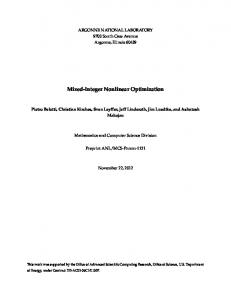
ysp is the set point of the outputs and k is the tuning parameter for desired closed-loop responses. Fig. 1 shows the closed-loop control implementation of the nonlinear model-based controller.
(21)
(22)
where S0 is the initial substrate concentration (kg/m3) of the medium, S is the final substrate concentration (kg/m3) of the medium, P is the final product concentration (kg/m3) of the medium and BT is the batch time (s) allocated for the fermentation process. Combining equations (12-17) with the macro scale bioreactor model of (18-22), we obtain a kinetics hybrid model of the fermentation process.
Figure 1. Nonlinear Model-Based Controller.
Note that when there are no constraints, i.e. (26) and (27) do not exist, the optimal solution for the nonlinear optimization will have an explicit form as follows: T
Δu t* = −[Δy t − k ∫ ( y sp − y mt )dt ] 0
28
(29)
which is a PI type controller, but the gain is adjusted using the nonlinear model of (23) so it is nonlinear gain.
50
AR SS
sp Controller
20 10
Biomass Conc. (g/L solution)
0
0
20
60
+10% So, D -10% So, D
60 50 40 30 20 10
0
20
40 Time (hr)
Biomass Conc. Substrate Conc. Product Conc.
60
80
+10% So, D -10% So, D
0.4
0.2
0
80
70
D
Bioreactor
40 Time (hr)
Product Conc. (g/L solution)
So
Productivity (g/L.hr)
A. Control Objective The control design objective was to maintain yield and productivity of the fermentation process in the face of disturbances in the feed substrate concentration So and or dilution rate, D. Fig. 2 outlines the feedback control of the fermentation process, where sp is the set point of the output variables, i.e. productivity and yield. Yield and productivity will be calculated based on the measured biomass, product and substrate concentrations.
30
Substrate Conc. (g/L solution)
Yield (%)
V. SIMULATION RESULTS
0.6
+10% So, D -10% So, D
40
0
20
40 Time (hr)
60
80
80 +10% So, D -10% So, D
70 60 50 40 30
0
20
40 Time (hr)
60
80
15 +10% So, D -10% So, D 10
5
0
0
20
40 Time (hr)
60
80
Figure 2. System Layout of Fermentation Process.
Figure 3. Open-Loop Dynamics of Yield, Productivity, Biomass Concentration, Substrate Concentration and Product Concentration.
B. Open-Loop Dynamics Table I summarizes the steady state conditions for all the input, output and disturbance variables, whereas Table II shows the disturbance variables values after step perturbation of +10% around their operating conditions.
Furthermore, we notice that the dynamics of substrate concentration is the fastest as compared to that of biomass and product concentrations. Thus, only slight changes in substrate concentrations are observed after the initial period. C. Closed- Loop Dynamics In the closed-loop analysis, we implement the nonlinear controller designed using either the data-based or the hybrid kinetics model to control both yield and productivity in the fermentation process. We study their performances in the face of disturbance scenario as in Table II. Fig. 4 shows that both controllers were able to keep the controlled variable in their set-point values, by manipulating both AR and SS. A step change of +10% was made in S0 and D at time t=20 hr (72,000s), i.e. both S0 and D values were changed instantaneously to a new value and kept constant at this new value indefinitely. From Fig. 4, it can be seen that both controllers performed well, whereby there are not much oscillations observed in the closed-loop dynamics of the yield. More dynamics are observed for the productivity. The kinetics hybrid model controller showed a bit of oscillations with higher overshoot and required longer time to return to the set-point. On the other hand, the performance of the simple data-based controller is slightly better.
TABLE I: SUMMARY OF STEADY STATE CONDITIONS FOR ALL VARIABLES
TABLE II: +10% STEP VARIABLES (SCENARIO I) Description So D
Steady State Condition 21.15% 0.15g/L.hr (4.17x10⁻⁵kg/m3.s) 30g/L solution (30kg/m3 solution) 48g/L solution (48kg/m3 solution) 5.2g/L solution (5.2kg/m3 solution) 1.43LPM (2.38x10⁻⁵m3/s) 250rpm (4.17rps)
PERTURBATION
Up 55 1.1
VALUES
OF
DISTURBANCE
Down 45 0.9
The open-loop dynamics of the fermentation process were simulated and analyzed. Fig. 3 shows their open loop dynamics to the disturbance changes. As observed in Fig. 3, the dynamics of productivity is faster than the dynamics of yield. Based on the responses of the magnitude, this analysis shows that the yield and productivity can also be controlled by manipulating S0. Same goes to biomass, substrate and product concentrations, whereby these can be controlled by the manipulation of S0. However, our system does not allow S0 to be manipulated variable.
50 Data-Based Model Kinetics Hybrid Model
Yield (%)
40
Productivity (g/L.hr)
Description Yield Productivity Biomass Concentration Substrate Concentration Product Concentration AR SS
30 20 10 0
29
0
20
40 Time (hr)
60
80
Data-Based Model Kinetics Hybrid Model
0.6 0.4 0.2 0
0
20
40 Time (hr)
60
80
1.5
10
0
20
40 Time (hr)
60
80
0
0
20
40 Time (hr)
60
5
0
0
20
40 Time (hr)
60
2 1 0 0
80
20
40 Time (hr)
60
Stirrer Speed (rpm)
400 Data-Based Model Kinetics Hybrid Model 300
200
100
0
20
40 Time (hr)
60
80
60
Data-Based Model Kinetics Hybrid Model
50 40 30 20 10
0
20
40 Time (hr)
60
0.6 0.3 0
80
60
80
0
20
40 Time (hr)
60
80
80 Data-Based Model Hybrid Kinetics Model
70 60 50 40 30
0
20
40 Time (hr)
60
80
15 Data-Based Model Kinetics Hybrid Model 10
5
0
0
20
40 Time (hr)
Stirrer Speed (rpm)
The results indicate that for the 10% change of disturbances, a simple controller performs slightly better than that of the complex, hybrid controller. Such differences are not significant, though. Both control strategies were able to keep the controlled variables in their set-point values for the 10% change of the disturbances. Our investigation is continued for a larger disturbance scenario exciting more nonlinearity and dynamics of the process. The step perturbation was increased to +30% from the steady state conditions of S0 and D as in Table III.
60
80
Data-Based Model Kinetics Hybrid Model
3 2 1 0 0
20
40 Time (hr)
60
80
Data-Based Model Kinetics Hybrid Model 300
200
100
0
20
40 Time (hr)
60
80
Figure 5. Closed-Loop Responses for Disturbance Scenario II.
As a conclusion, the kinetics hybrid model-based controller produces a much better closed-loop performance as compared to the data-based controller, especially when the fermentation process experiences more dynamics and nonlinearity as demonstrated by a higher step perturbation. This is because the kinetics hybrid model could capture the nonlinear dynamics of the process. However, if the disturbance is not “big”, the simple data-based controller should be sufficient.
TABLE III. +30% STEP PERTURBATION VALUES OF DISTURBANCE VARIABLES (SCENARIO II) Up 65 1.3
40 Time (hr)
0.9
400
Figure 4. Closed-Loop Responses for Disturbance Scenario I.
Description So D
20
80
Product Conc. (g/L solution)
10
Data-Based Model Kinetics Hybrid Model
3
0
80
15 Data-Based Model Kinetics Hybrid Model
20 10
40 30
Productivity (g/L.hr)
50
30
Substrate Conc. (g/L solution)
20
60
Data-Based Model Kinetics Hybrid Model
1.2
Aeration Rate (LPM)
30
Data-Based Model Kinetics Hybrid Model
70
Data-Based Model Kinetics Hybrid Model
40 Yield (%)
40
80
Biomass Conc. (g/L solution)
50
Substrate Conc. (g/L solution)
Data-Based Model Kinetics Hybrid Model
Aeration Rate (LPM)
Product Conc. (g/L solution)
Biomass Conc. (g/L solution)
50
60
Down 35 0.7
Fig. 5 shows the closed-loop responses for both databased and kinetics hybrid model-based controllers for scenario II. Both control strategies were able to maintain the controlled variables in the set point values. However, the kinetics hybrid model controller performed much better than the data-based model controller. Much more oscillations and demanded longer period of settling time to bring the process back to the set point are observed for the data-based controller. This could be seen for all the input and output variables. Besides, a higher overshoot can be observed especially for yield, productivity, biomass concentration and substrate concentration. Note that the manipulated variables AR and SS hit their upper limits indicating nonlinear dynamics of the process.
VI. CONCLUSION A new model-based control design for non-ideally mixed fermentation process has been presented in this paper. Models with different complexity were employed for the controller design. The disturbances of the inlet substrate concentration, S0 and dilution rate, D, were simulated to study the effectiveness of the designed nonlinear controllers. Our study has revealed that the choice of the nonlinear controller would depend on the expected disturbances on the process. For a relatively small disturbance scenario, the data-based controller should be sufficient; however, for a significantly large disturbance, the kinetics hybrid modelbased controller was able to enhance the closed-loop performance.
30
ACKNOWLEDGMENT The author gratefully acknowledges all parties who had supported and contributed in this research for their time and effort. REFERENCES [1]
[2]
[3] [4]
[5]
[6]
C.B. Youssef, V. Guillou and A. Olmos-Dichara, “Modelling and adaptive control strategy in a lactic fermentation process,” Control Engineering Practice, vol. 8, pp. 1297-1307, 2000. J.F. Van Impe and G. Bastin, “Optimal Adaptive Control of FedBatch Fermentation Processes,” Control Eng. Practice, vol. 3, pp. 939-954, 1995. K. Schügerl and K.H. Bellgardt, Bioreaction Engineering: Modeling and Control, Springler-Verlag Berlin Heidelberg, 2000, pp. 145. L.W.T. Emily, J. Nandong and Y. Samyudia, “Optimization of Fermentation Process Using a Multi-Scale Kinetics Model,” Proc. 5th International Symposium on Design, Operation and Control of Chemical Processes (PSE Asia 2010), July 2010, pp. 1174-1183, ISBN.978-981-08-6395-1. S. Starzak, M. Krzystek, L. Nowicki and H. Michalski, “Macroapproach kinetics of ethanol fermentation by Saccharomyces cerevisiae: experimental studies and mathematical modelling,” The Chemical Engineering Journal, vol. 54, pp. 221-240, 1994. T. Firmansyah and Y. Samyudia, Robust Nonlinear Control Systems Design, Lambert Academic Publishing, 2010.
31