KSCE Journal of Civil Engineering (2011) 15(5):831-840 DOI 10.1007/s12205-011-1154-4
Geotechnical Engineering
www.springer.com/12205
Nonlinear Neural-Based Modeling of Soil Cohesion Intercept Ali Mollahasani*, Amir Hossein Alavi**, Amir Hossein Gandomi***, and Azadeh Rashed**** Received March 1, 2010/Revised May 30, 2010/Accepted October 17, 2010
···································································································································································································································
Abstract A new model was derived to estimate undrained cohesion intercept (c) of soil using Multilayer Perceptron (MLP) of artificial neural networks. The proposed model relates c to the basic soil physical properties including coarse and fine-grained contents, grains size characteristics, liquid limit, moisture content, and soil dry density. The experimental database used for developing the model was established upon a series of unconsolidated-undrained triaxial tests conducted in this study. A Nonlinear Least Squares Regression (NLSR) analysis was performed to benchmark the proposed model. The contributions of the parameters affecting c were evaluated through a sensitivity analysis. The results indicate that the developed model is effectively capable of estimating the c values for a number of soil samples. The MLP model provides a significantly better prediction performance than the regression model. Keywords: soil cohesion intercept; soil physical properties; artificial neural networks; nonlinear modeling ···································································································································································································································
1. Introduction One of the most important engineering properties of soil is its ability to resist sliding along internal surfaces within a mass. The stability of structures built on soil depends on the shearing resistance offered by the soil along probable surfaces of slippage. The shear strength of geotechnical materials is generally represented by the Mohr-Coulomb theory. According to this theory, the soil shear strength varies linearly with the applied stress through two shear strength components known as cohesion intercept and angle of shearing resistance. The values of these empirical parameters for any soil depend on several factors such as the soil textural properties, past history of soil, initial state of soil, and permeability characteristics of soil (Poulos, 1989; Al-Shayea, 2001; Murthy, 2008). If the cohesion intercept and angle of shearing resistance are determined using the total stresses, they are named as total or undrained cohesion intercept (c) and angle of shearing resistance (φ ). If the pore water pressures are measured during the test, the effective strength parameters (c' and φ' ) are obtained. Accurate determination of c is a major concern in the design of different geotechnical structures such as foundations, slopes, underground chambers, and open excavations. This key parameter can be determined either in the field or in the laboratory. The triaxial compression and direct shear tests are the most common tests for determining the c values in the laboratory. The triaxial
test is more suitable for clayey soils. The direct shear test is commonly used for sandy soils and requires simpler test procedure in comparison with the triaxial test. The tests employed in the field include vane shear test or any other indirect method (Murthy, 2008; El-Maksoud, 2006). However, experimental determination of c is extensive, cumbersome, and costly. Also, it is not always possible to conduct the tests on every new situation. In order to cope with such problems, numerical solutions have been developed to estimate the shear strength parameters. The fact that most of the available empirical models are based on limited experimental data rises doubts on their generality. On the other hand, despite the multivariable dependency of soils, such correlations are mostly developed using only one soil index property. Incorporating simplifying assumptions into the development of the statistical and numerical methods may also lead to very large errors (Panwar and Seimens, 1972; Korayem et al., 1996; Terzaghi et al., 1996; Shahin et al., 2001). By extending developments in computational software and hardware, several alternative computer-aided data mining approaches have been developed. Pattern recognition systems, as an example, learn adaptively from experiences and extract various discriminators. Artificial Neural Networks (ANNs) (Haykin, 1999) are the most widely used pattern recognition methods. Some of the recent scientific efforts directed at applying ANNs to geotechnical engineering problems include extracting soil constitutive behavior (Hashash and Song, 2008), modeling of maximum dry
****Researcher, Dept. of Civil Engineering, Ferdowsi University of Mashhad, Mashhad, Iran (E-mail:
[email protected]) ****Researcher, School of Civil Engineering, Iran University of Science and Technology, Tehran, Iran (Corresponding Author, E-mail: ah_alavi@hotmail. com) ****Lecturer, College of Civil Engineering, Tafresh University, Tafresh, Iran (E-mail:
[email protected]) ****Researcher, Dept. of Civil Engineering, Ferdowsi University of Mashhad, Mashhad, Iran (E-mail:
[email protected]) − 831 −
Ali Mollahasani, Amir Hossein Alavi, Amir Hossein Gandomi, and Azadeh Rashed
density and optimum moisture content of stabilized soil (Alavi et al., 2009, 2010), simulating saltwater intrusion process in coastal aquifers (Bhattacharjya et al., 2008), compressive strength prediction of stabilized soil (Heshmati et al., 2009), and prediction of lateral behavior of single and group piles (Kim et al., 2008). Recently, Kayadelen et al. (2009) developed an ANN model to predict the φ ' value of soils. Multilayer Perceptron (MLP) (Cybenko, 1989) is an alternative ANN approach. MLP is essentially capable of approximating any continuous function to an arbitrary degree of accuracy (Cybenko, 1989). This approach is useful in deriving an empirical model for characterizing the undrained shear strength parameters by directly extracting the knowledge contained in the experimental data. In this paper, the MLP technique has been utilized to obtain a precise model relating c to several physical properties of soils. The proposed model was developed based on triaxial tests conducted in this study. ANNs are commonly considered as black box systems as they are unable to explain the underlying principles of prediction. To overcome this limitation, a conventional calculation procedure is further proposed based on the fixed connection weights and bias factors of the best MLP structure.
2. Artificial Neural Network Artificial Neural Networks (ANNs) have emerged as a result of simulation of biological nervous system. The ANN method was founded in the early 1940s by McCulloch and co-workers (Perlovsky, 2001). The first researches were focused on building simple neural networks to model simple logic functions. At the present time, ANNs can be applied to problems that do not have algorithmic solutions or problems with complex solutions. ANN formulates a mathematical model for a system in which no clear relationship is available between the inputs and outputs. Unlike the majority of the conventional statistical methods, ANNs use the data alone to determine the structure of the model and the unknown model parameters. The ability of ANNs to learn by example makes them very flexible and powerful techniques. Thus, this approach has widely been applied to solving regression and classification problems in many fields. 2.1 Multilayer Perceptron Network MLPs are class of ANNs using feedforward architecture. These networks are universal approximators because of their essential capability of approximating any continuous function to an arbitrary degree of accuracy (Cybenko, 1989). MLPs are usually applied to perform supervised learning tasks, which involve iterative training methods to adjust the connection weights within the network. They are usually trained with Back Propagation (BP) (Rumelhart et al., 1986) algorithm. Fig. 1 shows a schematic representation of an MLP network. The MLP networks consist of an input layer, at least one hidden layer of neurons and an output layer. Each of these layers has several processing units and each unit is fully interconnected with the weighted con-
Fig. 1. A Schematic Representation of an MLP Network
nections to units in the subsequent layer. Each layer contains a number of nodes. Every input is multiplied by the interconnection weights of the nodes. Finally, the output (hj) is obtained by passing the sum of the product through an activation function as follows: hj = f ⎛⎝ ∑ xi wij + b⎞⎠
(1)
i
where f () is activation function, xi is the activation of ith hidden layer node, wij is the weight of the connection joining the j th neuron in a layer with the i th neuron in the previous layer, and b is the bias for the neuron. For nonlinear problems, sigmoid functions (Hyperbolic tangent sigmoid or log-sigmoid) are usually adopted as the activation function. Adjusting the interconnections between layers will reduce the following error function: 1 E = --- ∑ ∑ ( tkn–hkn )2 2n k
(2)
where t nk and hnk are respectively the calculated output and the actual output value, n is the number of sample and k is the number of output nodes. Further details of MLPs can be found in (Cybenko, 1989).
3. Experimental Study Triaxial compression test is presently the most widely used procedure for determining the shear strength parameters of soils. In the triaxial soil testing system, field conditions can efficiently be simulated since the confining pressure is applied to the soil specimen according to the uniform lateral in-situ stresses. With respect to the problem statement, three types of testing techniques can be applied, namely Unconsolidated Undrained (UU), Consolidated Undrained (CU), and Consolidated Drained (CD) (Kayadelen et al., 2009). Within the scope of this study, a series of unconsolidated, undrained, and unsaturated triaxial (UU) tests were performed in accordance with ASTM D2850-87 (1987) to determine the shear strength parameters of 81 different undisturbed soil samples. 3.1 Sampling A total of 50 drillings were performed at different locations in Khorasan and Khouzestan provinces, Iran. The soil samples were manually taken by divers from test pits using metal tubes, 4
− 832 −
KSCE Journal of Civil Engineering
Nonlinear Neural-Based Modeling of Soil Cohesion Intercept
and 6 inches in diameter. The samples were obtained at depths ranging from 5 to 30 m and contained no gravel or larger particles. After extracting, the cores were carefully taken to the geotechnical laboratory and maintained in a wet chamber to avoid loosing of water content. Undisturbed sub-samples were then extracted from the cores for the geotechnical characterization tests. Also, several disturbed soil samples were taken from the sites for other testing purposes. 3.2 Basic Geotechnical Characterization Tests Extensive geotechnical laboratory test programs were carried out for the basic characterization of the soil samples. These comprised determining water (or moisture) content, natural unit weight of the soil, Atterberg limits (plastic and liquid limits), and grain size distribution. The grain size distribution of the disturbed samples was determined by sieving from number 4, 8, 16, 30, 50, 100 and 200 sieves and for finer soils (silt and clay) remaining from the 200 sieves. A sedimentation test throughout a hydrometer analysis was also carried out. To avoid flocculation of the finer fraction, a dispersing agent (sodium hexametaphosfate) was added to the soil-water mixture before the sedimentation test. Fig. 2 illustrates the lower and upper limits of the grain size distribution of the samples tested. Different soil types tested were gravelly silt with sand (ML), sandy silt (ML), silty clay with sand (CL-ML), silt with sand (ML), lean clay (CL), silty sand with gravel (SM), poorly-graded gravel with clay (GP-GC), sandy silty clay (CL-ML), lean clay with gravel (CL), lean clay with sand (CL), gravelly lean clay with sand (CL), sandy silt with gravel (ML), and silt (ML).
Fig. 2. Lower and Upper Limits of the Grain Size Distribution of the Soil Samples
3.3 Triaxial Compression Tests The soil samples with dimension of 38-50 mm in diameter and 76-100 mm in height were used in the UU tests. The samples were enclosed in a thin rubber membrane and closed tightly using plastic O-rings from the top platen and base pedestal. Then, they were placed inside the water-filled cell. Afterwards, a known magnitude of confining pressure of the fluid was applied inside the cell. In order to obtain the soil failure, an axial stress was implemented on the top of the soil specimen by a frictionless ram through the top of the cell. Meanwhile, the axial stress applied and axial displacement of samples were measured by load cell until the samples fails. This test was repeated at least for three confining pressures. The obtained database includes measurements of fine (FC) and coarse-grained (CC) contents, grain size for which 30 percentage of the sample was finer (D30), coefficient of uniformity (Cu), liquid limit (LL), moisture content (W), dry density (γd), and bulk density (γ ). Undrained cohesion intercept (c) was also the measured soil shear strength parameter. Total of 81 data sets were considered for developing the prediction models. A major part of the database comprises the laboratory test results for finegrained soil samples. The descriptive statistics of the data used in this study are also given in Table 1. To visualize the distribution of the samples, the data are presented by frequency histograms (Fig. 3).
4. Modeling of Soil Cohesion Intercept Precise estimation of the undrained cohesion intercept is an essential criterion in design process of geotechnical tasks. Due to the complexity of the behavior of the soil strength parameters, it is not simple to identify a relationship between the involved parameters. Cohesion is mainly due to the intermolecular bond between the adsorbed water surrounding each grain, especially in fine-grained soils (Murthy, 2008; El-Maksoud, 2006). The soils with high plasticity like clayey soils have higher cohesion and lower angle of shearing resistance. Conversely, as the soil grain size increases like sands, the soil cohesion decreases. The main purpose of this study is to obtain a meaningful MLPbased relationship between c and the influencing parameters. The most important factors representing the c behavior were detected based on the literature review (Mayne, 2001; Al-Shayea, 2001; Murthy, 2008; El-Maksoud, 2006; Kayadelen et al., 2009). The undrained cohesion intercept (c) (kg/cm2) was considered to
Table 1. Descriptive Statistics of the Variables used in the Model Development FC (%)
D30 (mm)
Cu
LL (%)
W (%)
γd (gr/cm3)
c (kg/cm2)
80.945
0.051
78.543
28.171
16.643
1.607
0.367
Standard Error
2.112
0.026
20.083
0.634
0.637
0.012
0.031
Standard Deviation
19.124
0.239
181.858
5.739
5.765
0.109
0.284
Minimum
9.6
0.001
2.14
20
3.5
1.37
0.02
Maximum
99.1
1.9
1150
46
30
1.81
1.16
Parameter Mean
Vol. 15, No. 5 / May 2011
− 833 −
Ali Mollahasani, Amir Hossein Alavi, Amir Hossein Gandomi, and Azadeh Rashed
Fig. 3. Histograms of the Variables used in the Model Development
W (%) : Moisture content γd (gr/cm3) : Soil dry density γ (gr/cm3) : Bulk density
be a function of several parameters as follows: c = f ( FC, CC, D30, Cu, LL, W, γd, γ )
(3)
where, FC (%) : Fine-grained content CC (%) : Coarse-grained content D30 (mm) : Grain size for which 30 percentage of the sample was finer : Coefficient of uniformity (D60 / D10). D10 and D60 Cu are grain sizes, in millimeters, for which 10 and 60 percentages of the sample was finer. LL (%) : Liquid limit
The significant influence of the above parameters in determining c is well understood. It is known that the cohesion intercept is affected by the basic soil properties (fabric characteristics), the state of the soil, and its consolidation history. FC, CC, D30, Cu, and LL represent the intrinsic soil properties. W, γd and γ provide information on the state of the soil and its previous history. They are also indicators of void ratio. OverConsolidation Ratio (OCR) could have been included in the analysis. OCR was not used herein as it should be obtained from
− 834 −
KSCE Journal of Civil Engineering
Nonlinear Neural-Based Modeling of Soil Cohesion Intercept
time-consuming laboratory tests. On the other hand, γd and γ can easily be calculated for a soil. 4.1 Performance Measures Correlation coefficient (R), root mean squared error (RMSE) and mean absolute percent error (MAPE) were used to evaluate the performance of the proposed models. R, RMSE and MAPE are given in the form of equations as follows: n
∑ i = 1( hi – hi )( ti – ti )
R = ---------------------------------------------------------------n
2
n
∑ i = 1( hi – hi ) ∑ i = 1( ti – ti )
(4)
2
Xn = ax + b
i=1
(5)
n
hi – ti 1 - × 100 MAPE = --- ∑ -----------hi n
(6)
i=1
where hi and ti are respectively the actual and predicted output values for the ith output, hi is the average of the actual outputs, and n is the number of sample. It is well known that the R value alone is not a good indicator of prediction accuracy of a model. The reason is that R will not change by equally shifting the values predicted by a model. RMSE is one of the most popular measures of error. It has the advantage that large errors receive much greater attention than small errors. MAPE is commonly used in quantitative prediction methods because it produces a measure of relative overall fit (Hecht-Nielson, 1990). MAE and the RMSE can be used together to diagnose the variation in the errors in a set of estimates. Higher R values and lower RMSE and MAPE values indicate a more precise model. 4.2 Data Preprocessing Some of the soil property variables are fundamentally interdependent. The first step in the analysis of interdependency of the data is to make a careful study of what it is that these variables are measuring, noting any highly correlated pairs. High positive or negative correlation coefficients between the pairs may lead to poor performance of the models and difficulty in interpreting the effects of the explanatory variables on the response. This interdependency can cause problems in analysis as it will tend to exaggerate the strength of relationships between variables. This is a simple case commonly known as the problem of multicollinearity (Dunlop and Smith, 2003). It is apparent that there is a high negative correlation between FC and CC. Also, γd and γ are highly correlated with each other. There will be no advantage of having both variables in the modeling process as one can represent the other. Thus, decisions were made to remove the correlated parameters in order to maximize the reliability of the final model. Vol. 15, No. 5 / May 2011
(7)
where,
n
∑ ( hi – ti ) 2 RMSE = -------------------------- × 100 n
For the MLP analysis, the data sets were randomly divided into training and testing subsets. Training data were used for learning. The testing data were used to measure the performance of the MLP models on data that played no role in building the models. Out of the available data, 69 data vectors were used for the training process and 12 data were taken for the testing of the models. In order to obtain a consistent data division, several combinations of the training and testing sets were considered. Both the input and output variables were normalized in this study. After controlling several normalization methods (Swingler, 1996; Mesbahi, 2000), the following method was used to normalize the variables to a range of [L, U] :
U–L a = -----------------------Xmax – Xmin
(8)
b = U – aXmax
(9)
in which Xmax and Xmin are the maximum and minimum values of the variable and Xn is the normalized value. In the present study, L = 0.05 and U = 0.95. 4.3 Model Development using MLP The available database was used for establishing the MLP prediction models. After developing different models with different combinations of the input parameters, the final explanatory variables (FC, D30, Cu, LL, W, γd) were selected as the inputs of the optimal model. For the development of the MLP models, a script was written in the MATLAB environment using Neural Network Toolbox 5.1 (MathWorks, 2007). The performance of an ANN model mainly depends on the network architecture and parameter settings. According to a universal approximation theorem (Cybenko, 1989), a single hidden layer network is sufficient for the traditional MLP to uniformly approximate any continuous and nonlinear function. Choosing the number of the hidden layers, hidden nodes, learning rate, epochs, and activation function type plays an important role in the model construction. Hence, several MLP network models with different settings for the mentioned characters were trained to reach the optimal configurations with the desired precision (Eberhart and Dobbins, 1990). The written program automatically tries various numbers of neurons in the hidden layer and reports the R, RMSE and MAPE values for each model. The model that provided the highest R and lowest RMSE and MAPE values on the training data sets was chosen as the optimal model. Various training algorithms were implemented for the training of the MLP network such as gradient descent (traingd), Levenberg–Marquardt (trainlm), and resilient (trainrp) back propagation algorithms. The best results were obtained by Quasi-Newton back-propagation (trainbfg) method. Also, log-sigmoid was adopted as the transfer function between the input and hidden layer. The transfer function between the hidden layer and output layer was a linear
− 835 −
Ali Mollahasani, Amir Hossein Alavi, Amir Hossein Gandomi, and Azadeh Rashed
Cu, LL, W, γd) and a bias term; One invariant output layer with 1 node providing the value of c. ● One hidden layer having 6 (m = 6) nodes.
transfer function (purelin). The ANN toolbox in MATLAB randomly assigns the initial weights and biases for each run each time (MathWorks, 2007). These assignments considerably change the performance of a newly trained ANN even all the previous parameter settings and the ANN architecture are kept constant. This leads to extra difficulties in the selection of the optimal ANN architecture and parameter settings. To overcome this difficulty, the weights and biases were frozen after the network was well trained and then the trained ANN model was translated into explicit forms (Guzelbey et al., 2006; Tapkýn et al., 2009). For brevity, the detailed explanations of the procedure used to convert the optimal ANN model into simple equation is not given.
●
The explicit formulation of c is as follows: Vi ⎞ 1 c ( kg/cm 2 ) = ---------------- ⎛ – 3.1895 + ∑ --------------0.7895 ⎝ 1 + e –F ⎠ i where, Fj = FCn × W1i + D30n × W2i + Cun × W3i + LLn × W4i + Wn × W5i + γdn × W6i + Biasi , i = 1, ..., 6
(11)
in which, FCn, D30n, Cu,n, LLn, Wn, and γd,n respectively represent the inputs variables normalized using Eq. (7). i is the number of the hidden layer neurons. The input layer weights (Wi), input layer biases (Biasi), and hidden layer weights (Vi) of the optimum MLP model are presented in Tables 2 and 3. The MLP model was built with a learning rate of 0.05 and trained for 1,500 epochs. Comparisons of the predicted versus experimental c values are shown in Fig. 4.
4.4 MLP-based Formulation for Soil Cohesion Intercept The model architecture that gave the best results for the formulation of the undrained cohesion intercept (c) was found to contain: ●
(10)
j
One invariant input layer, with 6 (n = 6) arguments (FC, D30,
Table 2. Weight and Bias Values between the Input and Hidden Layer Number of hidden neurons (i) Weights
1
2
3
4
5
6
W1i
9.8772
4.1858
1.9700
9.8601
12.5035
-11.1453
W2i
2.0136
-2.1360
-8.6685
1.9825
-0.8749
2.0077
W3i
-5.2599
13.5814
13.2740
-3.1667
0.7696
3.8014
W4i
0.1009
8.8448
10.9255
-1.7578
3.3352
-7.7729
W5i
10.8502
2.7682
-24.8648
36.8155
0.8320
-13.6760
W6i
-4.0653
-4.4922
2.8089
-0.3596
-1.2803
15.0461
Biasi
0.3397
-2.6089
1.9675
3.1940
-1.5186
-0.7549
Table 3. Weight Values between the Hidden and Output Layer Number of hidden neurons (i) Weights
1
2
3
4
5
6
Vi
9.3120
-7.3948
-3.9038
-3.9087
0.8777
2.1238
Fig. 4. Predicted versus Experimental c Values using the Best MLP Model: (a) Training Data, (b) Testing Data − 836 −
KSCE Journal of Civil Engineering
Nonlinear Neural-Based Modeling of Soil Cohesion Intercept
4.5 Model Development Using Regression Analysis A multivariable nonlinear least squares regression (NLSR) (Ryan, 1997) analysis was performed to have an idea about the predictive power of the best MLP model, in comparison with a classical statistical approach. The method of NLSR is extensively used in the regression analyses because of its interesting nature. Under certain assumptions, NLSR has some attractive statistical properties that have made it as a member of the most powerful and popular methods of the regression analysis. NLSR extends the linear least-squares regression for use with a much larger and more general class of functions. There are very few limitations on the way parameters can be used in the functional part of the nonlinear regression models (Ryan, 1997). The NLSR prediction equation relates c to the predictor variables as follows: α + α5 Cuα + α7 LLα + α9 W a + α11 γda + α13 c = α1 FC α + α3 D30 (12) 2
4
6
8
10
12
where α denotes coefficient vector. The NLSR model was trained using the same training and testing data sets previously considered for developing the MLP model. Eviews software package (Maravall and Gomez, 2004) was used to perform the regression analysis. The NLSR-based formulation of c in terms of FC, D30, Cu, LL, W, and γd is as given below: 8.504 cNLSR ( kg/cm 2 ) = – 2500.89 FC –.00008 + 0.003D30
+ 0.0692Cu0.213 – 10.108LL –0.851 + 3175.22W–0.0001 + 1892.33 γd0.0006 – 2566.23
(13)
Comparisons of the predicted versus experimental c values are shown in Fig. 5.
5. Performance Analysis of the Models A precise prediction model was developed for the soil cohesion intercept upon a reliable database. A comparison of the ratio between the predictions made by the MLP and NLSR models and the experimental c values is shown in Fig. 6. No rational model has been found for the prediction of c that encompasses the influencing variables considered in this study. Thus, it was not possible to conduct a comparative study between the results of this research and those in hand. Based on a logical hypothesis (Smith, 1986; Kasabov, 1998), if a model gives R > 0.8, and the RMSE and MAPE values are at the minimum, there is a strong correlation between the predicted and measured values. The model can therefore be judged as very good. It can be observed from Fig. 4 that the MLP model with high R and low RMSE and MAPE values is able to predict the target values to an acceptable degree of accuracy. Meanwhile, it is noteworthy that the RMSE values are not only low but also as similar as possible for the training and testing sets. This suggests that the proposed model has both predictive ability (low values) and generalization performance (similar values) (Pan et al., 2009). The 95% confidence interval of the predicted soil cohesion values for the entire data was 0.058. The models derived using ANNs or other soft computing tools have a predictive capability within the data range used for their
Fig. 5. Predicted versus Experimental c Values using the NLSR Model: (a) Training Data, (b) Testing Data
Fig. 6. Comparison of the c Predictions Made by Different Models for the Entire Database Vol. 15, No. 5 / May 2011
− 837 −
Ali Mollahasani, Amir Hossein Alavi, Amir Hossein Gandomi, and Azadeh Rashed
development. For these methods, the amount of data involved in the modeling process is an important issue, as it bears heavily on the reliability of the final models. To cope with this issue, Frank and Todeschini (1994) argue that the minimum ratio of the number of objects over the number of selected variables for model acceptability is 3. They also suggest that it is more reasonable to consider a ratio equal to 5. In the present study, this ratio is higher and is equal to 81/6 = 13.5. The above facts ensure the derived prediction model is valid and is not a chance correlation. It is obvious that, in all cases, the MLP model has a remarkably better performance than the NLSR model. Empirical modeling based on statistical regression techniques has significant limitations. Most commonly used regression analyses can have large uncertainties. It has own major drawbacks pertaining idealization of complex processes, approximation and averaging widely varying prototype conditions. Contrary to MLP, the regression-based methods model the nature of the corresponding problem by a pre-defined linear or nonlinear equation.
6. Sensitivity Analysis Sensitivity analysis is of utmost concern for selecting the important input variables. The contribution of each input parameter in the MLP model was evaluated through a sensitivity analysis. To achieve this, relative importance values of the predictor variables were calculated using Garson's algorithm (Garson, 1991). Fig. 7 presents a summary of the Garson’s protocol for determining the relative importance values. According to this algorithm, the input-hidden and hidden-output weights of the trained MLP model were partitioned and the absolute values of the weights were taken to calculate the relative importance values. The relative importance values of the input parameters of the MLP model are presented in Fig. 8. According to these results, it can be found that c, for the ranges investigated,
Fig. 8. Contributions of the Predictor Variables in the MLP Model
is more dependent on Cu and γd compared with the other soil properties. Another observation from the results of the sensitivity study is that W is less important in explaining the variations of the c values.
7. Conclusions In this research, a high-precision model was derived for assessing the undrained soil cohesion intercept, c, using the MLP paradigm. The proposed model was developed based on well established and widely dispersed triaxial test results obtained through an experimental study. The following principal conclusions may be drawn based on the results presented: • The developed MLP model gives reliable estimates of the c values. The results indicate that the proposed model possesses some obvious superiority in comparison with the nonlinear regression model. • Contrary to the conventional models, the proposed model simultaneously takes into account the role of several important factors (FC, D30, Cu, LL, W, and γd) representing the behavior of the shear strength parameters. The results indicate that W and γd are efficient representatives of the initial state and
Fig. 7. Determining the Relative Importance of Each Input Variable using the Garson’s Algorithm (Alavi et al., 2010) − 838 −
KSCE Journal of Civil Engineering
Nonlinear Neural-Based Modeling of Soil Cohesion Intercept
•Step 2: Calculation of the hidden layer. The input value of each neuron in the hidden layer is determined for six neurons using the input layer weights and biases shown in Table 2. Given the information provided, the input values of the neuron (F1,…, F6) are calculated using Eq. (11):
consolidation history of the soil. • The sensitivity analysis results indicate that Cu and γd are the most important parameters governing the behavior of c. • The proposed model is mostly suitable for fine-grained soils with physical properties similar to the soil samples used in this study. The model can be improved to make more accurate predictions for a wider range by adding newer data sets for other soil types and test conditions. • The tractable MLP-based design equation provides an analysis tool accessible to practicing engineers. The MLP calculation procedure outlined in Appendix A can readily be performed using a spreadsheet or hand calculations to give predictions of the c values. • Using the MLP approach, the c values can be estimated without carrying out sophisticated and time-consuming laboratory or field tests. • A major distinction of MLP for determining the c values lies in its powerful ability to model the mechanical behavior without assuming prior form of the existing relationships.
F1 = 9.8772×0.5407+4.1858×0.0604+1.9700×0.1110 +9.8601×0.1538+12.5035×0.3105−11.1453×0.7864 +0.3397 = 2.7860 (15) Similarly, F2 = -0.9993, F3 = 4.1586, F4 = -0.3519, F5 = -3.0788, and F6 = 8.4668. •Step 3: Prediction of c. The input value of each output neuron is calculated using an activation function (log-sigmoid function). The calculated values are multiplied by the hidden layer connection weights (Table 3) and the summation is obtained: A = 9.3121f(F1)−7.3948f(F2) −3.9038f(F3) −3.9087f (F4) (16) + 0.8777f (F5)+ 2.1238 f (F6) = 3.4856
Further research can be focused on analyzing the relationships between the angle of shearing resistance and the soil physical properties using the MLP technique. This leads to the formulation of a power and nonlinear model for friction angle like the ones derived for the cohesion in this work.
where f(x) is the a log-sigmoid function of form 1/(1+e−x). Using Eq. (10), the value of c is calculated as follows: 1 c = ---------------- ( – 3.1895 + 3.4861 ) = 0.375 kg/cm 2 0.7895
Appendix. Design Example An illustrative design example is provided to further explain the implementation of the soil cohesion intercept formula. For this aim, one of the soil samples used for the testing of the model was taken. The FC, D30, Cu, LL, W, and γd values for the sample are respectively equal to 58.4%, 0.023 mm, 80, 23%, 11.1%, and 1.73 gr/cm3. The c of the soil is required. The calculation procedure can be divided into three sections: 1) normalization of the input data, 2) calculation of the hidden layers, and 3) prediction of c. The calculation procedure is outlined in the following steps: • Step 1: Normalization of the input data (FC, D30, Cu, LL, W, γd) to lie in a range from 0.05 to 0.95 and calculation of the input neurons (FCn, D30,n, Cu,n, LLn, Wn, γd,n) for each input data vector using Eqs. (7) to (9). The input neurons are calculated as: For FC: the maximum and minimum values of the variable are 99.1 and 9.6, thus: 0.95 – 0.05 0.95 – 0.05 FCn = ⎛ -------------------------⎞ FC + ⎛ 0.95 – ------------------------- × 99.1⎞ ⎝ 99.1 – 9.6 ⎠ ⎝ ⎠ 99.1 – 9.6
(14)
= 0.5407 Similarly, D30,n = 0.0604, Cu,n = 0.1110, LLn = 0.1538, Wn = 0.3105, and γd,n = 0.7864. Vol. 15, No. 5 / May 2011
(17)
In this example, the result is in good agreement with the experimental value (0.37 kg/cm2) of c as it yields a value 1.35% higher.
References Alavi, A. H., Gandomi, A. H., Mollahasani, A., Heshmati, A. A. R., and Rashed, A. (2010). “Modeling of maximum dry density and optimum moisture content of stabilized soil using artificial neural networks.” J. Plant. Nutr. Soil. Sci., Vol. 173, No. 3, pp. 368-379. Alavi, A. H., Gandomi, A. H., Gandomi, M., and Sadat Hosseini, S. S. (2009). “Prediction of maximum dry density and optimum moisture content of stabilized soil using RBF neural networks.” The IES J. Part A . Civ. Struct. Eng., Vol. 2, No. 2, pp. 98-106. Al-Shayea, N. A. (2001). “The combined effect of clay and moisture content on the behavior of remolded unsaturated soils.” Eng. Geol., Vol. 62, No. 4, pp. 319-342. ASTM D2850-87. (1987). Standard test method for unconsolidated, undrained compressive strength of cohesive soils in triaxial compression. Bhattacharjya, R. K., Datta, B., and Satish, M. G. (2009). “Performance of an artificial neural network model for simulating saltwater intrusion process in coastal aquifers when training with noisy data.” KSCE J. Civ. Eng., Vol. 13, No. 3, pp. 205-215. Cybenko, J. (1989). “Approximations by superpositions of a sigmoidal function.” Math. Cont. Sign. Syst., Vol. 2, pp. 303-314. Dunlop, P. and Smith, S. (2003). “Estimating key characteristics of the concrete delivery and placement process using linear regression analysis.” Civil Eng. Environ. Syst., Vol. 20, pp. 273-290.
− 839 −
Ali Mollahasani, Amir Hossein Alavi, Amir Hossein Gandomi, and Azadeh Rashed
Eberhart, R. C. and Dobbins, R. W. (1990). Neural network PC tools, A Practical Guide, Academic Press, San Diego, C.A. El-Maksoud, M. A. F. (2006). “Laboratory determining of soil strength parameters in calcareous soils and their effect on chiseling draft prediction.” Proc. Energy Efficiency and Agricultural Engineering Int. Conf., Rousse, Bulgaria. Frank, I. E. and Todeschini, R. (1994). “The data analysis handbook.” Elsevier, Amsterdam, The Nederland. Garson, G. D. (1991). “Interpreting neural-network connection weights.” AI Expert, Vol. 6, No. 7, pp. 47-51. Guzelbey, I. H., Cevik, A., and Gogus, M. T. (2006). “Prediction of rotation capacity of wide flange beams using neural networks.” J. Constr. Steel Res., Vol. 62, No. 10, pp. 950-961. Hashash, M. A. and Song, H. (2008). “The integration of numerical modeling and physical measurements through inverse analysis in geotechnical engineering.” KSCE J. Civ. Eng., Vol. 12, No. 3, pp. 165-176. Haykin, S. (1999). Neural networks - A comprehensive foundation, 2nd Ed., Prentice Hall Inc., Englewood Cliffs. Hecht-Nielson, R. (1990). “Neurocomputing.” Reading, Mass: AddisonWesley. Heshmati, A. A. R., Alavi, A. H., Keramati, M., and Gandomi, A. H. (2009). “A radial basis function neural network approach for compressive strength prediction of stabilized soil.” Geotech. Spec. Pub. ASCE., Vol. 191, pp. 147-153. Kasabov, N. K. (1998). Foundations of neural networks fuzzy systems and knowledge engineering, MIT Press, Cambridge. Kayadelen, C., Günaydýn, O., Fener, M., Demir, A., and Özvan, A. (2009). “Modeling of the angle of shearing resistance of soils using soft computing systems.” Expert Syst. Appl., Vol. 36, pp. 1181411826. Kim, B. T., Kim, Y. S., and Lee, S. H. (2008). “Prediction of lateral behavior of single and group piles using artificial neural networks.” KSCE J. Civ. Eng., Vol. 5, No. 2, pp. 185-198. Korayem, A. Y., Ismail, K. M., and Sehari, S. Q. (1996). “Prediction of soil shear strength and penetration resistance using some soil properties.” Mis. J. Agr. Res., Vol. 13, No. 4, pp. 119-140. Maravall, A. and Gomez, V. (2004). Eviews software, Version 5, Quantitative Micro Software, LLC, Irvine C.A.
MathWorks (2007). Inc. MATLAB the language of technical computing, Version 7.4, Natick, MA, U.S.A . Mayne, P. W. (2001). “Stress-strain-strength-flow parameters from enhanced in-situ tests.” Proc., In-Situ Measurement of Soil Properties & Case Histories, Bali, Indonesia, pp. 27-48. Mesbahi, E. (2000). Application of artificial neural networks in modelling and control of diesel engines, PhD Thesis, University of Newcastle, U.K. Murthy, S. (2008). Geotechnical engineering. principles and practices of soil mechanics, 2nd Edition, Taylor & Francis, CRC Press, U.K. Pan, Y., Jiang, J., Wang, R., Cao, H., and Cui, Y. (2009). “A novel QSPR model for prediction of lower flammability limits of organic compounds based on support vector machine.” J. Haz. Mater., Vol. 168, Nos. 2-3, pp. 962-969. Panwar, J. S. and Seimens, J. C. (1972). “Shear strength and energy of soil failure related to density and moisture.” T. ASAE, Vol. 15, pp. 423-427. Perlovsky, L. I. (2001). Neural networks and intellect, Oxford University Press. Poulos, S. J. (1989). “Liquefaction related phenomena.” Advance Dam Engineering for Design, Construction, and Rehabilitation, Van Nostrand Reinhold, pp. 292-297. Rumelhart, D. E., Hinton, G. E., and Williams, R. J. (1986). “Learning internal representations by error propagation.” Proc., Parallel Distributed Processing, MIT Press, Cambridge. Ryan, T. P. (1997). Modern regression methods, Wiley, New York, N.Y. Shahin, M. A., Maier, H. R., and Jaksa, M. B. (2001). “Artificial neural network applications in geotechnical engineering.” Aus. Geomech. Vol. 36, No. 1, pp. 49-62. Smith, G. N. (1986). Probability and statistics in civil engineering, Collins, London. Swingler, K. (1996). Applying neural networks a practical guide, Academic Press, New York, N.Y. Tapkýn, S., Cevik, A., and Usar, Ü. (2009). “Accumulated strain prediction of polypropylene modified marshall specimens in repeated creep test using artificial neural networks.” Exp. Syst. Appl., Vol. 36, pp. 11186-11197. Terzaghi, K., Peck, R. B., and Mesri, G. (1996). Soil mechanics in engineering practice, 2nd Ed., Wiley & Sons, Inc., New York, N.Y.
− 840 −
KSCE Journal of Civil Engineering