Nonlinear Preconditioning in Problems of Optimal ... - Math.mcmaster.ca

Nonlinear Preconditioning in Problems of Optimal Control for Fluid Systems Bartosz Protas * *

Department of Mathematics & Statistics, McMaster University, Hamilton, Ontario, Canada Abstract This note discusses certain aspects of computational solution of optimal control problems for fluid systems. We focus on approaches in which the steepest descent direction of the cost functional is determined using the adjoint equations. In the first part we review the classical formulation by presenting it in the context of Nonlinear Programming. In the second part we show some new results concerning determination of descent directions in general Banach spaces without Hilbert structure. The proposed approach is illustrated with computational examples concerning a state estimation problem for the 1D Kuramoto–Sivashinsky equation.

1

Introduction

Problems of optimal control arise in very many areas of science and engineering. φ) = 0, where x is the state of the system Given a (possibly nonlinear) system u(x,φ and φ is an actuation, control problems consist in determining the control φ , so that this control and the corresponding state minimize some performance criterion, i.e., φ) min J˜ (x,φ

x∈X ,φφ∈U

φ) = 0, subject to u(x,φ

(1a) (1b)

where U represents the set of admissible controls, whereas X is the space of system states. Applications of such problems in Fluid Mechanics are ubiquitous. Here we mention just some of the most important examples, admitting that this list is far from being exhaustive: • shape optimization with application to aircraft design, e.g., Mohammadi and Pironneau (2001); Martins et al. (2004), • flow control for drag reduction, e.g., Bewley et al. (2001); Protas and Styczek (2002), • variational data assimilation in dynamic meteorology, e.g., Kalnay (2003),

1

• mixing enhancement. In the above examples the performance criterion J˜ and the control φ may take different forms reflecting the structure of the problem at hand. The equation (1b) governing the state of the system is usually some form of the Navier–Stokes equation. In fact, from the formal point of view, optimal control problems are examples of inverse problems [see, e.g., Isakov (1997)]. In practice, problems of the type (1) involving minimization of a cost functional subject to some constraints are solved using optimization methods. Since the constraint is a partial differential equation (PDE), such problems are examples of PDE–constrained optimization. One of the first studies to analyze systematically such problems was the seminal work by Lions (1968). In the context of Fluid Mechanics these problems were further investigated by Abergel and Temam (1990) and Gunzburger (2002). When such infinite–dimensional problems are solved in practice, suitable discretization is used to obtain a corresponding finite– dimensional problem which, at least in principle, can be solved using methods of Nonlinear Programming (NLP). There are, however, some aspects of the problem that make this approach quite challenging. First of all, since the discrete systems are obtained from discretizations of PDEs, the dimension of the discrete state vector x can be extremely large. Consequently, it is impossible to store the linear operators involved in the solution process as matrices. Consequently, many existing software packages designed to solve finite–dimensional NLP problems cannot be used and “matrix–free” alternatives have to be developed. Secondly, given the size of the discrete system and difficulties involved in calculating second–order derivatives of the cost functional, the Hessian information is usually unavailable and Newton’s method can rarely be used. Consequently, one needs to use first– order (gradient) approaches such as, for instance, the Conjugate Gradient (CG) method. Moreover, the physical systems of interest to us are often characterized by a broad range of interacting length– and time–scales and, as a result, the optimization problem is very poorly conditioned. The purpose of the present paper is to discuss some recent ideas useful for accelerating convergence of iterative solution to such optimization problems. In particular, we will focus on nonlinear preconditioning strategies which, by performing locally a nonlinear change of the metric, attempt to increase the range of validity of the tangent linear approximation which is crucial to the present approach. The structure of the paper is as follows: in the next Section we introduce a simple, yet relevant from the Fluid Mechanics perspective, optimization problem based on the Kuramoto–Sivashinsky equation that we will use as our “toy model”, then we present a standard adjoint–based optimization approach typically used to solve such problems; in Section 3 we will introduce the idea of nonlinear preconditioning and show how it can be formulated in terms of gradient extraction in spaces without Hilbert structure; in Section 4 we will present some computational

2

results indicating the utility of the proposed method; conclusions and discussion of further perspectives are deferred to Section 5. The present report is of a rather exploratory nature, and more complete results concerning this problem are already available in Protas (2008).

2

Adjoint–Based Optimization

Here we show how problem (1) can be efficiently solved using methods of Nonlinear Programming. In its initial formulation this is a constrained optimization problem in which both the state x and the control φ are variables to be optimized. This is a rather inconvenient situation, since x is a solution of a (time–dependent) PDE and its discretization may contain a very large number of degrees of freedom in space and in time. On the other hand, the state x may be considered a function of the control, i.e., x = x(φφ), which allows us to express problem (1) in the corresponding unconstrained form φ ) = min J (φφ), min J˜ (x(φφ),φ

(2)

φ ∈U

φ ∈U

where J : U → R is called the reduced cost functional1. An advantage of this formulation over (1) is that now optimization is carried out with respect to one variable only with discretization usually involving much fewer degrees of freedom. Moreover, problem (2) is unconstrained so that optimization methods required to solve it are simpler, however, the price to be paid for this is that the functional dependence of J on φ is now much more involved. As mention in Introduction, we are concerned here with situations where calculation of the Hessian of (2) is impossible or impractical. We will therefore focus on first–order gradient–based methods. The necessary condition characterizing the minimum of the cost functional J (φφ ) is the vanishing of its Gˆateaux differential J ′ : U × U → R, i.e. J ′ (φφopt ;φφ′ ) = 0, ∀φφ′ ∈ U , (3) φ′ ) = limε→0 J (φφ+εφφε)−J (φφ) and where the Gˆateaux differential is defined as J ′ (φφ ;φ φ opt is the minimizer. In most applications, and also in the case considered here, the cost functional J˜ is quadratic in both x and φ , however, x = x(φφ) is often a nonlinear mapping and the optimization problem (2) may be therefore nonconvex. As a result, it may admit nonunique solutions and (3) will characterize only a local minimizer φopt . Given some initial guess φ (0) , such a minimizer can be found using gradient–based descent method of the general form ′

φ (k+1) = φ (k) + d(k) , k = 1, 2, . . . ,

(4)

1 Since this is the formulation we will focus on below, hereafter we will skip the adjective “reduced”,

unless needed for clarity.

3

such that limk→∞ φ (k) = φ opt , where k is the iteration count. At every iteration k the descent direction d(k) is determined based on the gradient ∇ J of the cost functional calculated at φ (k) . As will be shown below, this gradient can be extracted from J ′ (φφ(k) ;φφ′ ). A convenient expression for J ′ (φφ(k) ;φφ′ ) can be found using methods of Nonlinear Programming [see Lewis (2001) for a discussion of NLP techniques in the context of PDE–constrained optimization] E E E D D D ′ ˜ ,φ ˜ , (Dφ x)φφ ′ φ J ′ (φφ;φφ′ ) = Dφ J ,φφ′ = D J + D J , (5) x φ ∗ ∗ ∗ U ×U

U ×U

X ×X

where Da F denotes the Fr´echet derivative of the mapping F = F(a) [see Berger (1977)]. In (5) U ∗ is the dual space with respect to U and h·, ·iU ×U ∗ represents the standard duality pairing between the spaces U and U ∗ . Below we will show how the cost functional differential in (5), and in particular the term Dφ J , can be expressed using an appropriately–defined adjoint state. Using the implicit function theorem, the term Dφ x can be expressed as Dφ x = −(Dx u)−1 Dφ u,

(6)

so that the second term on the RHS in (5) can be transformed as follows E E D D ˜ , (Dx u)−1 Dφ uφ φ′ φ′ J = − D Dx J˜ , (Dφ x)φ x ∗ X ×X ∗ D D E E X ×X ∗ ′ ˜ ,φ φ φ′ , D x D J = − Dφ∗ u (Dx u)−∗ Dx J˜ ,φ x φ ∗ U ×U

U ×U ∗

,

(7) where an asterisk denotes a Banach space adjoint. Putting together (5) and (7) we see that the adjoint operator Dφ∗ x : X ∗ → U ∗ can be used to express the differential of the cost functional (5) in a convenient form as E D E D ′ φ J ′ (φφ;φφ′ ) = Dφ J˜ + Dφ∗ x Dx J˜ ,φφ′ = D J ,φ . (8) φ ∗ ∗ U ×U

U ×U

As is evident from the above relationship, the first argument in the duality pairing can be identified with the gradient of the reduced cost functional J : U → R in the metric induced by the space U . It must be emphasized that the gradient in fact belongs to the dual space Dφ J ∈ U ∗ and, since in most infinite–dimensional cases the dual space U ∗ is not contained in the original space U , this gradient may not be used as a descent direction in U . In the special case when U is a Hilbert space we can invoke Riesz’ representation theorem [Berger (1977)] which allows us to map Dφ J ∈ U ∗ to the corresponding element ∇ J ∈ U as D

J ′ (φφ;φφ′ ) = Dφ J ,φφ′

E

4

U ×U ∗

  φ′ , = ∇ J ,φ U

(9)

where (·, ·)U represents the inner product on the Hilbert space U , so that now ∇ J ∈ U can be used to construct a descent direction in U . On the other hand, when U is not a Hilbert space, Riesz’ theorem does not apply and identification (9) is not possible. However, in Section 3 we will present a method for constructing an equivalent of ∇ J in the space U in such a general case. Now we illustrate these somewhat abstract considerations by analyzing a concrete example of PDE–constrained optimization. We will focus on a model problem introduced in Protas et al. (2004) which concerns estimation of the initial condition for the 1D Kuramoto–Sivashinsky equation. This particular problem is selected as it models the variational data assimilation, known as 4DVAR, in Dynamic Meteorology [see Kalnay (2003)]. The Kuramoto–Sivashinsky equation is chosen, since it is endowed with chaotic and multiscale behavior and as such is an attractive model for the Navier–Stokes system. We follow here Protas et al. (2004) as regards the set–up of this problem and below highlight only the main points of the derivation, while the Reader is referred to the original source for further details. For simplicity, we will consider the 1D Kuramoto–Sivashinsky equation on a periodic spatial domain Ω = [0, 2π] and a time interval [0, T ]
 4 2   ∂t v + 4∂x v + κ ∂x v + v ∂x v = 0, x ∈ Ω, t ∈ [0, T ], (10) t ∈ [0, T ], i = 0, . . . , 3, . ∂ix v(0,t) = ∂ix v(2π,t),   v(x, 0) = φ, x ∈ Ω. Given incomplete and possibly noisy measurements y = H vact + η ∈ Y , where vact (·,t) ∈ X is the actual system trajectory, H : X → Y is an observation operator and η is (Gaussian) noise, our optimization problem consists in finding an initial condition φ in (10) such that the corresponding system trajectory best matches the available measurements y. In other words, we minimize the following cost functional Z

2 1 T 1

(H v(φ) − y)2 dτ. (11) = J (φ) = H v(φ) − y 2 2 0 L2 (0,T ;L2 (Ω)) Consistently with the properties of system (10), we will assume that φ ∈ U = L2 (Ω). Since J depends on the control variable φ implicitly through the state equation (10), expression (11) represents in fact the reduced cost functional [cf. (2)]. We will assume that the observation operator H has the form of projection on a set of cosine modes with the wavenumbers in some set Λr , i.e.  Z 2π  1 ′ ′ ′ H = ∑ Pr , where Pr z = cos(rx )z(x )dx cos(rx). (12) π 0 r∈Λr The Gˆateaux differential of (11) is given by [cf. (5)]

J ′ (φ; φ′ ) =

Z T Z 2π 0

(H v − y)H v′ dx dt,

0

5

(13)

where the perturbation v′ (φ; φ′ ) is obtained by solving the Kuramoto–Sivashinsky equation linearized around the state φ, i.e.   2 ′  ′ ′ 4 ′ ′ ′   L v = ∂t v + 4∂x v + κ ∂x v + v ∂x v + (∂x v) v = 0, x ∈ Ω, t ∈ [0, T ], ∂ix v′ (0,t) = ∂ix v′ (2π,t), t ∈ [0, T ], i = 0, . . . , 3,   ′ ′ v (x, 0) = φ , x ∈ Ω, (14) with the operator L : X → X ∗ understood in the weak sense. Relation (13) can now be transformed to a form consistent with (8) by introducing an adjoint operator L ∗ : X → X ∗ and the corresponding adjoint state v∗ ∈ X ∗ via the following identity E E D D ∗ ∗ ′ v∗ , L v′ = L v , v + bL . (15) ∗ ∗ X ×X

X ×X

Using integration by parts and the definition of L in (14), we obtain
L ∗ v∗ = −∂t v∗ + 4∂4x v∗ + κ ∂2x v∗ − v ∂x v∗ , and Z 2π t=T ∗ ′ bL = v v dx . 0

(16)

t=0

We remark that bL does not contain any boundary terms (resulting from integration by parts), since all of them vanish due to periodicity. Defining an adjoint system as  ∗ ∗ ∗ x ∈ Ω, t ∈ [0, T ],   L v = H (H v − y), i ∗ i ∗ (17) ∂x v (0,t) = ∂x v (2π,t), t ∈ [0, T ], i = 0, . . . , 3,   ∗ v (x, T ) = 0, x ∈ Ω,

and using (14), (15) and (16) we can now express the Gˆateaux differential (13) in the desired form (5) Z 2π v∗ φ′ dx. (18) J ′ (φ; φ′ ) = 0

t=0

Thus, this differential (i.e., the sensitivity of the cost functional J with respect to perturbations of the initial condition) can be expressed using the solution of the adjoint system (17). Relationship (18) can now be employed to extract the gradient required in a descent optimization algorithm. Since U = L2 (0, 2π), we immediately obtain

J ′ (φ; φ′ ) =

Z 2π 0

v∗

t=0

  φ′ φ′ dx = ∇ L2 J ,φ

L2 (Ω)

=⇒ ∇ L2 J = v∗

t=0

.

(19)

Despite its simplicity, in many cases this is not an optimal choice, as it may result in poor conditioning of the corresponding discrete optimization problem. In Protas

6

et al. (2004) a set of regularization options was identified which can, at least partially, alleviate some of such difficulties. In relation to gradient extraction it was shown that it can be beneficial to extract the cost functional gradient in a more general Hilbert space, Sobolev spaces being natural candidates [see also Neuberger (1997)]. In particular, gradient extraction was considered in the Sobolev space H 1 (Ω) characterized by the inner product Z 2π h   i 1 2 z1 , z2 1 = z z + l (∂ z ) (∂ z ) dx, (20) 1 2 x 1 x 2 2 H (Ω) (1 + l22 ) 0   1 φ′ where l2 is an adjustable length–scale. Identification J ′ (φ; φ′ ) = ∇ H J ,φ 1 H (Ω)

1

yields, after integration by parts, the gradient ∇ H J defined via solutions of the following Helmholtz boundary value problem   H1 1   ∗ 2 2  J = v ¯ ∇ 1 − l ∂ , 2 x t=0 1 + l22 (21)  1  H1 H ∇ J (0) = ∇ J(2π). 1

Thus, the Sobolev space gradient ∇ H J is obtained by applying the inverse Helmholtz operator to the classical L2 gradient. Interestingly, when regarded in Fourier space, the inverse Helmholtz operator is equivalent to a low–pass filter with the cut–off given by the inverse of the length–scale l2 parametrizing the inner product (20). Consequently, extracting gradients in Sobolev spaces with inner products given by (20) has the effect of de–emphasizing components with characteristic length–scales smaller than l2 . As was shown in Protas et al. (2004), adjusting this length–scale during solution of an optimization problem can accelerate convergence of iterations. In particular, starting with l2 large and then progressively decreasing it to zero results in a multiscale procedure targeting first the large–scale structures and then homing in on smaller scale components of the solution φopt .

3 Nonlinear Preconditioning using Descent Directions in General Banach Spaces In this Section we address the issue of gradient extraction in general Banach spaces and the potential advantage this technique may offer as a method of nonlinear preconditioning. Similar ideas were already discussed by Lewis (2001) and elaborated in greater detail by Neuberger (1997), however, they were not concerned with preconditioning nonlinear optimization problems. The present approach relies on the assumption that the Banach space U , where the descent direction is to be identified, be reflexive, i.e., that U ∗∗ = U . As already mentioned in Section 2 in relation

7

to formula (9), the gradient is a linear functional on the space U and therefore 1,p belongs to the dual space U ∗ . For example, if U is the Sobolev space W0 , p 6= 2, defined as W01,p (Ω) = {u : Ω → R, kukW 1,p < ∞, v|∂Ω = 0}, Z 1/p (22) p p p where kukW 1,p = (|v| + l p |∂x v| ) dΩ , Ω

∈ R+

where l p is a weight, then the dual space U ∗ = W −1,q , where 1p + 1q = 1 [see Adams and Fournier (2005)]. Since a dual space is usually “larger”, its elements do not necessarily belong to the original space U and therefore cannot be used to represent descent directions in that space. Consequently, it is necessary to propose φ′ ) a different approach which allows one to extract a descent direction g˜ from J ′ (φφ;φ such that g˜ ∈ U . As shown by Lewis (2001) and Neuberger (1997), this can be done defining g˜ as a unit–norm element of U which minimizes expression (9). In other words, we postulate to find g˜ as a solution of the following constrained minimization problem D E min Dφ J , g ∗ (23) U ×U

kgkU =1

which can be converted to the more convenient unconstrained form D  E µ p = min G (g), min Dφ J , g ∗ + kgkU g∈U g∈U U ×U p

(24)

where p is an integer, µ is the Lagrange multiplier and G : U → R. This problem can be solved with a method analogous to the approach described earlier in Section 2. Thus, the descent direction g˜ is characterized by the vanishing of the Gˆateaux differential of (24), i.e. E D ∀g′ ∈U G ′ (˜g; g′ ) = Dg G (˜g), g′ ∗ = 0, (25) U ×U

where Dg G : U

→ U∗.

Thus, we obtain

Dg G (˜g) = 0 in U ∗

(26)

as an equation determining the direction g˜ ∈ U . Below we will show how this direction can be determined when U is one of the Banach spaces commonly arising in the analysis on nonlinear PDEs. This analysis will be carried out in the setting of the optimization problem for the Kuramoto–Sivashinsky equation introduced in Section 2. We begin with the Lebesgue spaces L p (Ω) with norms defined as [Adams and Fournier (2005)]  Z 1/p   |u| p dΩ 1 ≤ p < ∞, kukL p (Ω) = (27) Ω   ess supx∈Ω |u| p = ∞. 8

Considering for the moment the case with 1 ≤ p < ∞, the unconstrained cost functional (24) and its Gˆateaux differential (25) take the form Z µ G (g) = (v∗ t=0 g + |g| p ) dΩ, (28a) p Ω Z (28b) ∀g′ ∈L p (Ω) G′ (g; g′ ) = (v∗ t=0 g + µg|g|(p−2))g′ dΩ, Ω

so that the descent direction g˜L p is characterized by the algebraic relation 1 g| ˜ g| ˜ (p−2) = − v∗ t=0 . µ

The solution of (29) is  s  1  p−1  − v∗ t=0 ,   µ g˜ L p = s   1    − sgn(v∗ t=0 ) p−1 v∗ t=0 , µ

(29)

p — even, (30) p — odd.

We thus see that when p 6= 2, the descent direction in L p (Ω) is obtained by applying a nonlinear transformation to the original gradient ∇ L2 J = v∗ |t=0 . In the special case p = 2 we immediately obtain 1 g˜ L2 = − v∗ t=0 (31) µ

which is the classical expression obtained in Section 2. As regards the constant µ, which serves as a Lagrange multiplier in the unconstrained formulation (24), it is chosen to normalize g˜ to unit norm kgk ˜ U = 1. In the second special case p = ∞, it can be shown that g˜ L∞ = − sgn(v∗ t=0 ) (32)

consistently with taking the limit p → ∞ in expressions (30). We also remark that in the case p = 1 the descent direction g˜L1 cannot be defined, since the space L1 (Ω) is not reflexive. We now proceed to discuss the problem of determining the descent direction when U = W 1,p , where W 1,p is the Sobolev space defined in (22). Considering the case 1 ≤ p < ∞, the unconstrained cost functional and its Gˆateaux differential take the form  Z  µ G (g) = v∗ t=0 g + (|g| p + l pp |∂x g| p ) dΩ, (33a) p Ω Z  i µh g|g|(p−2)g′ − l pp ∂x (∂x g|∂x g|(p−2))g′ dΩ. (33b) G ′ (g; g′ ) = v∗ t=0 g′ + p Ω

9

As before, the boundary terms due to integration by parts vanish because of periodicity of g˜ and g′ . Since the descent direction g˜ is characterized by G ′ (g; ˜ g′ ) = 0, ∀g′ ∈U , it can be obtained as a solution of the following problem in U ∗ (due to nondifferentiability of the absolute value function | · |, this equations is formulated in the weak sense)  i h 1  g| ˜ x g| ˜ (p−2) = − v∗ t=0 , ˜ g| ˜ (p−2) − l pp∂x (∂x g)|∂ µ (34)  g(0) ˜ = g(2π). ˜

The second term on the LHS in the first equation in (34) is usually referred to as the p–Laplacian [Neuberger (1997)], as it represents a nonlinear generalization of the familiar Laplace operator. Evidently, in the case p = 2, W 1,2 (Ω) = H 1 (Ω) is a Hilbert space and the p–Laplacian reduces to the classical Laplace operator. As a result, (34) simplifies to (21) and we recover the Hilbert space framework discussed in Section 2. The Lagrange multiplier µ can be adjusted in order to normalize the descent direction to the unit norm. We can conclude that identification of descent directions in Banach spaces (such as L p (Ω), or W 1,p (Ω), when p 6= 2) results in nonlinear transformations of the adjoint field v∗ |t=0 . As regards equations with the p–Laplacian operator such as (34), a variety of their interesting properties is discussed by Ishii and Loreti (2005) (see also references contained therein). We now comment briefly on the utility of extraction descent directions in general Banach spaces as a nonlinear preconditioning technique. The purpose of preconditioning is to modify the metric in which a given iterative process takes place, so as to accelerate convergence. For linear problems with quadratic functionals this can also be regarded as decreasing the condition number of the Hessian of the reduced cost functional. In such cases linear preconditioning techniques are efficient enough (in fact, in many situations there exist specific guidelines regarding the choice of an optimal preconditioner). However, for nonlinear problems linear preconditioning may not be sufficient and a nonlinear change of the metric may lead to better results. In the framework proposed here, choosing a preconditioner is in fact equivalent to choosing a Banach space U in which the descent direction is identified. The question of how to choose this space is important. Unlike certain linear problems, most nonlinear PDEs result in optimization problems with structure that is too complicated to allow for a thorough analysis. In such situations finding the most suitable preconditioning strategy is a matter of experimentation. There are, however, certain general conditions that need to be satisfied. In general, for the evolution equation (10) to be well–posed, the control φ must belong to some appropriate space U (identical with L2 (Ω) in the present case). Therefore, if at the k–th iteration we want to precondition the gradient by extracting it (k) in some Banach space U (k) , it must be ensured that this gradient ∇U J will still

10

belong to the original space U , in other words U (k) ⊆ U , ∀k∈Z . Such preconditioning is equivalent to restricting the iterates to a family of subspaces nested in U . Computational results concerning linear preconditioning reported by Protas et al. (2004) indicate that the best results were obtained when the subspaces formed the following hierarchy

U (0) ⊆ U (1) ⊆ · · · ⊆ U (k) ⊆ · · · ⊆ L2 (Ω).

(35)

When considering general Banach spaces, additional guidance for constructing hierarchies like (35) can be obtained by considering the family of Sobolev Imbedding Theorems [Adams and Fournier (2005)]. Imbedding Theorems provide criteria that allow one to determine whether or not one Sobolev (or Lebesgue) space is “contained” in another one. In the following Section we present computational results that address some of these issues.

4

Computational Results

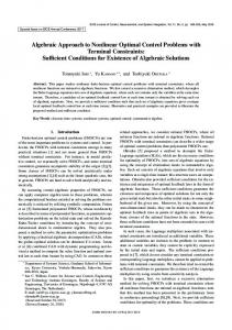
In this Section we show some computational results illustrating the utility of the nonlinear preconditioning techniques developed in Section 3. We treat the results from Protas et al. (2004) as our point of reference, so we consider here precisely the same problem of state estimation for the Kuramoto–Sivashinsky equation. The observation operator in (12) uses projections on the first r = 50 cosine modes (i.e., Λr = {1, . . . , 50}) and we set κ = 4000 in equation (10). Both equation (10) and its adjoint (17) are solved using a dealiased pseudo–spectral Fourier–Galerkin method with N = 1024 grid points. The Reader is referred to Protas et al. (2004) for further numerical details. The nonlinear equation (34) involving the p–Laplacian operator is solved using Newton’s method applied to the system of nonlinear algebraic equations obtained after discretization. In order to see the effect of nonlinear preconditioning we will present results obtained for two optimization horizons (given in terms of the time step ∆t = 10−8 ) T = 300 and T = 500. Since the effect of nonlinear preconditioning appears most pronounced for the longer optimization horizon T = 500, some of the results will be presented for that case only. We begin presentation of the results by examining the shape of the descent directions g˜ obtained in different Banach spaces. To fix attention, we consider the first iteration in the problem with T = 500 with a zero initial guess φ(0) ≡ 0. In Figure 1 we compare the descent directions g˜ extracted in the Banach spaces L2 (Ω), L∞ (Ω) and W 1,4 (Ω) with l4 = 10.0 [cf. (22)] with the standard gradient ∇L2 J extracted in the space L2 (Ω). We observe that for increasing p the descent directions obtained in the spaces L p (Ω) approach a square wave. In computational solution of our optimization problem we found the preconditioning involving descent directions in the Sobolev spaces W 1,p (Ω), where p ≥ 3,

11

g 0

/2

x

Figure 1. Shapes of the descent directions obtained at the first iteration in the data assimilation problem with T = 500 and determined in: (solid line) L2 (Ω), (dashed line) L5 (Ω), (dotted line) L∞ (Ω) and (dash–dotted line) W 1,4 (Ω). For clarity, only half of the domain Ω is shown.

to be more efficient than the preconditioning using descent directions in L p (Ω). This is the case we will focus on exclusively below. In Figures 2a and 2b, corresponding to optimization with T = 300 and T = 500, we study the effect that the quantity l p , the characteristic “length–scale” parametrizing the definitions of the norm kukW 1,p , has on optimization efficiency. Given that the value of the cost function (11) before optimization (i.e., for φ(0) ≡ 0) is normalized to unity, Figures 2a and 2b show the decrease of the cost functional at the first iteration for the descent directions obtained in the spaces W 1,3 (Ω) and W 1,4 (Ω) with values of l3 and l4 indicated on the abscissa. For comparison, we also show the results obtained with the gradient extracted in L2 . We note that the decrease of the cost functional significantly depends on the choice of l p (p = 3, 4). For T = 300 the window of l p giving improvement over optimization with the L2 gradients exists for descent directions in W 1,3 (Ω) only and is rather narrow. The advantage of determining descent directions in a Banach space becomes much more evident for T = 500, where the windows of l p giving improvement over gradients in L2 are unbounded. Now we proceed to analyze the effect of nonlinear preconditioning on the whole optimization process involving many iterations. As regards optimization with the descent directions obtained in the Banach spaces W 1,p (Ω) we follow the strategy outlined in Section 3: for a given choice of the space W 1,p (Ω) we start with the value of l p which was determined to give the best results at the first iter-

12

0.8 0.75

J

0.7 0.65 0.6 0.55 -2 10

2

3

4

5

-1 6 7 8 910

2

3

4

5

6 7 8 91

l3,l4 (a)

0.841667 0.833333

J

0.825 0.816667 0.808333 0.8 -2

10

2

5

-1

10

2

5

1

2

5

10

l3,l4 (b) Figure 2. Decrease of the cost functional (11) at the first iteration in optimization with (a) T = 300 and (b) T = 500. The descent directions are extracted in the spaces (solid line) L2 (Ω), (dashed line) W 1,3 (Ω) and (dotted line) W 1,4 (Ω) for values of l3 and l4 indicated on the abscissa.

13

ation and then progressively decrease it to zero, so that the corresponding descent directions approach the L p descent direction. As a result, our preconditioning strategy is equivalent to extracting the descent directions in a sequence of nested spaces W 1,p (Ω), all contained in the “master” space L2 (Ω). This strategy, initially investigated by Protas et al. (2004) for the case of gradient extraction in the Sobolev space H 1 (Ω) = W 1,2 (Ω), was found to give good results. In Figures 3a and 3b we show the decrease of the cost functional J (φ(k) ) as a function of the iteration count k for T = 300 and T = 500, respectively. In both cases the descent directions are extracted in the spaces W 1,4 (Ω) with the initial values of l4 equal to 10−1 and 10 in the two cases, respectively. For comparison, in the two Figures we also show the decrease of the cost functional obtained with gradients obtained in the space L2 (Ω). We note that when T = 300 nonlinear preconditioning offers little advantage over the unpreconditioned case, in contrast to the case with T = 500 where a significant convergence acceleration is observed. In order to further emphasize this point in Figures 4a and 4b we show the data for the error in the reconstruction of the initial condition, i.e., kφ(k) − φact kL2 (Ω) corresponding to the same cases as in Figure 3. We note that these results provide further evidence for the trends already shown in Figure 3. We also examined nonlinear preconditioning in the case of shorter optimization horizons T ≪ 300, however, no acceleration of convergence comparing to the optimization with the L2 gradients was observed. Hence, we do not show these results here.

5

Conclusions and Outlook

In this paper we first reviewed the formulation of an optimal control problem for a fluid system using the language of Nonlinear Programming. We focused on a particular aspect relevant from the computational point of view, namely, determination of well–preconditioned descent directions for the cost functional. We extended an earlier approach and showed how a descent direction can be determined in a general Banach space without Hilbert structure. In particular, we showed that extracting this descent direction in a Sobolev space W 1,p (Ω) leads to solution of an elliptic problem with a p–Laplacian. Such a preconditioning strategy has the effect of a nonlinear change of the metric in the space where optimization is performed. When employed judiciously, this approach may have the potential to mitigate the effect of nonlinearities present in the system. Indeed, our computational results indicate that such a nonlinear preconditioning can accelerate convergence of iterations in an optimization problem for a nonlinear PDE. Interestingly, effectiveness of the proposed approach increases with the length of the optimization interval [0, T ] and becomes more evident for problems with large T , i.e., in situations when nonlinear effects play a more significant role. Research is underway to apply a similar approach to precondition optimization of more realistic problems,

14

1 5

2

10

-1

J

5

2

10

-2 5

2

10

-3

0

10

20

30

40

50

60

70

80

90

100

iter

(a) 1

5

J

2

10

-1

5

0

500

1000

1500

2000

iter

(b) Figure 3. Decrease of the cost functional J (φ(k) ) in function of iterations for optimizations with (a) T = 300 and (b) T = 500. The results are obtained with the descent directions in (solid line) L2 and (dotted line) W 1,4 (Ω) where the parameter l4 progressively decreases with iterations.

15

1.0

0.8 0.7

||

(k)

-

act

||L2

0.9

0.6 0.5 0.4 0.3

0

10

20

30

40

50

60

70

80

90

100

k (iter)

(a) 1.0

0.8

0.7

||

(k)

-

act

||L2

0.9

0.6

0.5

0

500

1000

1500

2000

k (iter)

(b) Figure 4. Decrease of the error of the reconstruction of the initial condition kφ(k) − φact kL2 (Ω) in function of iterations for optimizations with (a) T = 300 and (b) T = 500. The results are obtained with the descent directions in (solid line) L2 and (dotted line) W 1,4 (Ω) where the parameter l4 progressively decreases with iterations.

16

such as the state estimation in a 3D turbulent channel flow already investigated by Bewley and Protas (2004). Another possibility is to investigate descent directions in more general Banach spaces and here Besov spaces [see, e.g., Adams and Fournier (2005)] are attractive candidates. A thorough treatment of this subject is given in Protas (2008). In the present investigation the space giving “optimal” preconditioning was chosen by trial and error. A very challenging theoretical question is to develop a rigorous procedure that will determine guidelines for choosing such an optimal space. Such procedures are in fact available for certain optimization problems formulated for some linear PDEs, however, no such results appear available for nonlinear PDEs. Encouraging computational results reported in the present paper may therefore serve to motivate further theoretical research in this direction.

6

Acknowledgments

This research has been supported by an NSERC (Canada) Discovery Grant.

Bibliography F. Abergel and R. Temam. On some control problems in fluid mechanics. Theoretical and Computational Fluid Dynamics, 1:303–325, 1990. R. A. Adams and J. J. F. Fournier. Sobolev Spaces. Elsevier, second edition edition, 2005. M. S. Berger. Nonlinearity and Functional Analysis. Academic Press, 1977. T. R. Bewley and B. Protas. Skin friction and pressure: the “footprints” of turbulence. Physica D, 196:28–44, 2004. T. R. Bewley, P. Moin, and R. Temam. DNS–based predictive control of turbulence: an optimal benchmark for feedback algorithms. Journal of Fluid Mechanics, 447:179–225, 2001. M. Gunzburger. Perspectives in Flow Control. SIAM, 2002. V. Isakov. Inverse Problems for Partial Differential Equations. Springer, 1997. H. Ishii and P. Loreti. Limits of solutions if p–laplace equations as p goes to infinity and related variational prblems. SIAM J. Math. Anal., 37:411–437, 2005. E. Kalnay. Atmospheric modeling, data assimilation and predictability. Cambridge University Press, 2003. R. M. Lewis. A nonlinear programming perspective on sensitivity calculations for systems goverened by state equations. Technical report, ICASE, 2001. J. L. Lions. Contrˆole optimal de syst`emes gouvern´es pas des e´ quations aux d´eriv´ees partielles. Dunod, 1968.

17

J. R. R. A. Martins, J. J. Alonso, and J. J. Reuther. High–fidelity aerostructural design optimization of a supersonic business jet. Journal of Aircraft, 41:523– 530, 2004. B. Mohammadi and O. Pironneau. Applied Shape Optimization for Fluids. Oxford University Press, 2001. J. Neuberger. Sobolev Gradients and Differential Equations. Springer, 1997. B. Protas. Adjoint–based optimization of pde systems with alternative gradients. Journal of Computational Physics, 227:6490–6510, 2008. B. Protas and A. Styczek. Optimal rotary control of the cylinder wake in the laminar regime. Physics of Fluids, 14:2073–2087,, 2002. B. Protas, T. Bewley, and G. Hagen. A comprehensive framework for the regularization of adjoint analysis in multiscale pde systems. Journal of Computational Physics, 195:49–89, 2004.

18