Nonlinear Projection for the Display of High Dimensional Distance Data. Dan Ashlock Mathematics and Statistics University of Guelph, Guelph, Ontario, N1G 2W1
[email protected]
A BSTRACT Display and visualization of high dimensional data are typically performed with a well-chosen linear projection of the data or by displaying many linear projections to form an animation. This study presents an evolutionary algorithm for producing non-linear projections of high dimensional data with cues, in the drawing of the projection, as to the types of distortions introduced. Such projection can provide drawings closer to the true high dimensional distances of the displayed data than any linear drawing. The system is demonstrated on a synthetic four dimensional fitness landscape and on distance data derived from RNA folds. Because fitness landscapes often have more dimensions than can be easily visualized it can be difficult to gain an intuitive understanding of a fitness landscape. The non-linear projection algorithm is applied to an abstraction of the fitness landscape called a fitness web. Fitness webs can be used to display the relative quality of optima, the frequency with which they were found by different evolutionary runs, or other factors of interest. In addition to displaying the relative position of optima in a fitness landscape, a graph of the fitness function along the edges a fitness web displays important slices of the fitness landscape. Called fitness morphs these plots can provide intuition about the fitness landscapes as well as direction for subsequent evolutionary searches. The second demonstration of the non-linear projection algorithm is to data generated from an ad-hoc metric on RNA folds. The algorithm correctly distinguishes two different types of folds for iron response elements.
Justin Schonfeld Bioinformatics and Computational Biology Iowa State University, Ames, Iowa 50011
[email protected]
morphs. Together these two visualizations export much of the information contained in the fitness landscape to an easily viewable format. Fitness webs and the non-linear projection algorithm for producing drawings of them have their genesis in an attempt to model a set of biological data, shown in Figure 1. In the process of assembling genomic sequences in corn a statistical anomaly appeared. When sequences were assembled there were apparent sequencing errors that displayed a statistical consistency. Two sequences that both have a “C” instead of an “A” in position 56 would also have a “G” instead of a “C” in position 124. Careful investigation showed that what had in fact happened, at least some of the time, was that two different genes with nearly identical sequences had been incorrectly merged by the genome assembly software. These odd genes are called nearly identical paralogs or NIPs. The apparent sequencing errors that pointed to NIPs appear at a rate low enough to be mistaken for sequencing errors if it were not for their coincidental agreement or correlation with other apparent sequencing errors within the assembly. We call these correlated “errors” coincident polymorphisms. The data shown in Figure 1 is the number of nearly identical paralogs identified thus far in corn put into bins by their number of coincident polymorphisms they posses.
CP Count
120
100
Number of NIPs
80
I. I NTRODUCTION Fitness landscapes were first introduces as a metaphor for the space in which the dynamics of evolution take place by Sewall Wright in 1932[11]. Informally, a fitness web is an abstraction of a fitness landscape to a combinatorial graph whose vertices are the (currently known) optima of the fitness landscape. We will use fitness webs to drive two distinct sorts of visualizations of a fitness landscape. The first are drawings of the fitness web that retain much of the information about the distances between the optima. The second are plots of the landscape along edges of the graph called fitness
60
40
20
0 0
5
10
15
20
25
Number of CPs
Fig. 1. Number of nearly identical paralogs found as a function of their number of coincident polymorphisms.
C(n) = e
−0.590n
(81.4 + 55.3n),
(1)
these valleys are not sufficient to explain the fact that the randomly initialized modeling software did not find the good model even once in 100 tries. The morph plot is, however, a cross section. The basin of attraction of the bad model is quite likely far larger in 4-space than shown in this 1-space slice of the modeling fitness landscape. The effect of mode on squared error 1000 error**2
800
Squared error
In order to model the data, an evolutionary algorithm was used to fit models of the form C(n) = e−an p(n) where C(n) is the predicted number of NIPs, n is the number of coincident polymorphisms, and p(n) is a polynomial. Models were fit with an evolutionary algorithm for various polynomial degrees with the idea that the degree where RMS error ceased to drop significantly would be the most nearly correct model. The goal was to predict the number of genes that were duplicated but exhibited no coincident polymorphisms. This is the only method, short of sequencing the corn genome, to estimate the dumber of duplicated but undifferentiated genes in corn. This predicted number of totally identical paralogs or TIPs is simply C(0) for a given model C(n). A problem arose. When the evolutionary algorithm was initialized with random model coefficients, the RMS error consistently rose from runs where the model C(n) = e−an · (b + cn) was fit to those runs where C(n) = e−an · (b + cn + dn2 ) was fit. Since simply setting d = 0 permits the former type of model to mimic the latter this is clearly an incorrect result. This incorrect result was found for 100 independent evolutionary model fits for both models. In addition the model fitting software was consistently finding the same models:
600
400
200
0 0
0.2
0.4
0.6
0.8
1
Morphing parameter
Fig. 2. A plot of the RMS error of the morph from before the bad model to after the good model along the line in R4 connecting them.The plot is jagged, we conjecture because of roundoff error associated with running relatively large values through the exponential function.
and C(n) = e−0.812n (75 + 71.7n + 21.6n2 ),
(2)
up to a modest amount of noise in the coefficients. The problem was not difficult to solve. Instead of randomly initializing the quadratic polynomials they were initialized to the values of the (superior) linear polynomials. Evolution was then able to locate a superior (lower RMS error) quadratic-exponential model for the data: C(n) = e−0.379n (125 − 9.16n + 2.23n2).
(3)
This problem in fitting the model is not unusual. An evolutionary algorithm was used for these model fits because the minimization of squared error for the polynomial-exponential model, unlike that for fitting a line or plane, is not linear. The problem is troubling, though, because it means the simple EA used to fit the model missed a better model 100 times in a row. On order to understand why this happened the following procedure was used. Both the good and bad quadratic-exponential models are given by four coefficients. If we think of these as ~ = (−0.379, 125 − 9.16, 2.23) and vectors in R4 , call then G ~ B = (−0.812, 75, 71.7, 21.6) for the good and bad models respectively, then by setting ~ (t) = t · G ~ + (1 − t)B, ~ V
(4)
then we can continuously change one model into the other. This process is called morphing between the models. A plot of the RMS error of the model V~ (t) as a function of the morphing parameter t is shown in Figure 2. If one ignores the numerical roundoff error that gives the plot a jagged appearance, a broad valley containing the bad model and a deeper narrow valley containing the good model are visible. The width ratios of
The outstanding problem, that the modeling software fit a clearly inferior model, was solved by tinkering with the initialization of the population of initial models. While trying to understand the failure of the algorithm the character of the model space’s fitness landscape shown in Figure 2 came to light. In the remainder of the paper we will develop tools for understanding such problems, include a non-linear drawing tool. The utility of this tool is demonstrated both for visualizing fitness landscapes and in a second application to visualizing the distances between a group of RNA folds. A. Fitness Webs A fitness web is an edge-weighted complete combinatorial graph. The vertices of the graph are a collection of optima found on some fitness landscape. The fitness web for the motivational model fitting problem has two vertices representing the good and bad optima. The position of the optima on the landscape is saved for future use. The edge weights are the distances between the optima in the independent variable space of the landscape. When real valued functions are being optimized the Euclidean distance in Rn . For other possible spaces, e.g. character strings, other distance measures will be required. The first goal of this research is to create a two-dimensional picture of the fitness web that comes as close as possible to giving the distances between optima. This is similar to a mapprojection problem, that of displaying the surface of a sphere (e.g. planet earth) on a flat map. The optima in n space have true distances between them and any projection of the optima into the plane for plotting has projected distances between the optima. The goal is to have the true and projected distances
agree as closely as possible while displaying at least the sign of the discrepancies between true and projected distances. Once a good projection is located the quality or other properties of the optima can be displayed on the fitness web giving at least some sense of the fitness landscape. The second goal is to provide additional information, possibly useful for subsequent search, by examining the fitness morphs along the lines joining optima in the fitness web. The number of morphs is quadratic 21 n(n − 1) in the number n of optima and so the fitness web can be used to investigate which morphs might be interesting to view and contain hints about where to focus additional searches of the fitness landscape. II. D ESCRIPTION
OF
T RIAL DATA S ETS
The first data set is derived from a landscape that is a sum of translates of the hill function: 1 f (x, y, z) = (5) 2 1 + x + y2 + z 2
{(16.0, 15.8, 11.8) (12.4, 14.2, 9.0) (15.5, 11.7, 11.4) (18.6, 15.5, 16.0) (3.9, 15.8, 10.1) (12.6, 2.6, 6.0) (17.8, 1.0, 10.7) (1.8, 14.3, 18.1}
set fi (x, y, x) = f (x−Pix , y−Piy , z −Piz ) where Pix , Piy , and Piz , refer to the x, y, and z coordinates of point i respectively. The demonstration surface is: S(x, y, z) =
7 X
C CA BBB BBBBB G ||| ||||| PPP-PPPPP U CG B form: UGC CA BBBB BBBBB G |||| ||||| PPPP-C-PPPPP U CG Fig. 3.
For each of the eight points: P0 P1 P2 P3 P4 P5 P6 P7
A form:
fi (x, y, z).
(6)
i=0
This yields a four dimensional hyper-surface with eight optima. Each of the optima is near, but not exactly on, the eight points used to displace the individual hill functions. We call the points the hill centers. If two hill centers are closer than √23 then they merge to form a single hill. The eight hills centers were chosen at random subject to the constraint that they were at least distance two from one another in the Euclidean metric on R3 . The second data set used to demonstrate the non-linear projection algorithm compares different folds of examples of an RNA motif. The RNA sequence data comprises six Ferritin Heavy Chain RNAs taken from Genbank with accession numbers gi-507251, gi-286151, gi-191071, gi-213691, gi-214135, gi-3559829. These sequences were chosen because they have been used in other evolutionary computation studies [2] and contain know secondary structure [4]. Each gene was scanned using the RNAMotif Software [5] for the presence of either of the two forms of the Iron Response Element (IRE) described by the literature. These two folds are shown in Figure 3. The B-P pairs shown may be any pair of RNA bases that
The two known folds for RNA of Iron Response Elements.
undergo Watson-Crick base pairing; they are not otherwise well conserved. The A form of the IRE fold has only a single base bulge between the two helices, while the B form has an internal loop. Due to the variable nature of the base pairs in the helices it is often difficult to locate RNA secondary structure motifs using traditional sequence based motif-search techniques. Five of the six genes contained the potential to form either of the two forms. The sixth gene, gi-3559829, possesses only the A form of the fold. For each of the eleven sequences an un-gapped alignment was constructed by aligning the first base of the IRE elements and adding the previous 8 bases and the necessary number of bases following the IRE to bring the total sequence length up to 81. These strings were then folded with the Mfold package [12], [7]. A binary string was then constructed from the folds, indexed by the set of all the possible pairs of bases in each sequence. The entries of this string were 1 if the bases indexing a position are not paired and 0 if they were not. A distance matrix was then constructed using Hamming distance on these length 3240 strings. Since most pairs of bases are not paired in any of the eleven strings the strings consist mostly of zeros. The actual Hamming distance matrix is given in Figure 4. This ad-hoc distance between RNA folds is intended to capture the structure while ignoring sequence variability. The accuracy of this metric is critically dependent on the correct alignment of the underlying RNA sequences. For the IRE sequences, which are short and have well know structure, this alignment is easy to obtain. In application to RNA motif search it will be necessary to find the alignments by some form of dynamic programming that incorporates sequence, position, and RNA-base pair status. Examples of such dynamic alignment algorithms appear in [6], [3], [8]. The Mfold software did not perfectly recover the IRE structures from the data and the distances located are the result of differences in the folds found by Mfold.
f1 f2 f3 f4 f5 f6 f7 f8 f9 f10 f11
f1
f2
f3
f4
f5
f6
f7
f8
f9
f10
f11
0 9 42 45 42 21 42 42 42 47 45
9 0 33 44 41 20 41 41 41 46 44
42 33 0 45 42 21 42 42 42 47 45
45 44 45 0 45 24 45 45 45 50 48
42 41 42 45 0 21 42 42 42 47 45
21 20 21 24 21 0 21 21 21 26 24
42 41 42 45 42 21 0 10 42 47 45
42 41 42 45 42 21 10 0 42 47 45
42 41 42 45 42 21 42 42 0 47 45
47 46 47 50 47 26 47 47 47 0 34
45 44 45 48 45 24 45 45 45 34 0
Fig. 4. Distance matrix for the six type A and five type B iron response element folds, f1 − F11 .
III. E XPERIMENTAL D ESIGN For the first data set a simple evolutionary optimizer operating on a population of 60 points in R3 , represented as arrays of real numbers, was used to locate the optima of Equation 6. The evolutionary optimizer used size four tournament selection, single point crossover, and uniform point mutation. The mutation operator added a number selected uniformly at random in the interval [−0.1, 0.1] to a single position in the gene. The small tournament size and relatively non-exploratory mutation operator were used to increase the probability the algorithm would locate bad optima. With larger population sizes or more reasonable mutation operators the optimizer did not find the lower quality optima. The optimizer was run 400 times and located the optima associated with the eight hill centers with frequencies given in Table I. The output of the optimizer together with the true distances between the optima located, form the input to the fitness web drawing software. Center P0 P1 P2 P3 P4 P5 P6 P7
Frequency 152 70 156 6 11 2 2 1
Fitness 1.153 1.125 1.146 1.086 1.050 1.048 1.045 1.032
TABLE I F REQUENCY OF LOCATION BY
A SIMPLE EVOLUTIONARY OPTIMIZER
TOGETHER WITH FITNESS OF THE OPTIMA ASSOCIATED WITH THE EIGHT HILL CENTERS FOR
E QUATION 6.
A drawing of the fitness web is an assignment of the optima that form the vertices of the fitness web to positions in the plane. The fitness of a drawing is the RMS error between the true and the projected distances, for all pairs of optima. An evolutionary algorithm was used to locate good drawings by minimizing this fitness. For Equation 6 each of the eight optima requires two coordinates in the plane yielding a sixteen dimensional optimization problem. The algorithm used to locate good drawings of the fitness web for Equation 6 is called the non-linear projection algorithm. It operates on a population of 100 length sixteen real arrays. The algorithm uses size seven tournament selection, two point crossover, and a mutation operator that
adds an unbiased bivariate Gaussian random variable to one of the eight points to which the optima are assigned. The standard deviation of this Gaussian mutation is one tenth the largest true distance between any two of the optima in the fitness web. This choice automatically scales the algorithm to the particular fitness web, although the choice of one-tenth as a scaling factor is arbitrary. Experiments on the second set of data were performed by applying the non-linear projection algorithm to the distance matrix given in Figure 4. The only change was from a sixteen to a twenty-two dimentional optimization problem as there were eleven RNA folds rather than eight optima. Instead of displaying the quality of optima the resulting diagram displays the type (A or B) of the RNA fold. IV. R ESULTS For both data sets the algorithm converged to a solution of some sort rapidly in each run. Runs to locate good pictures of the four dimensional fitness landscape produce only two drawings while the runs on the RNA-derived data produced a substantial diversity of drawings. We now examine the particulars for each set of data in more detail. A. Results for the four dimensional fitness landscape. Two drawings of fitness webs for Equation 6 are given in Figure 5. They display the relative fitness of the optima and the relative frequency of discovery for the optima, save that the minimum size of the circle corresponding to an optima is that sufficient to place a label on the optima. This minimum diameter is added to a number proportional to the quantity being displayed, fitness or frequency of discovery. There are three types of edges in the drawing. Short, dark edges are drawn between optima that have projected distances smaller than their real distances. Thin, light edges represent pairs of optima with projected distances greater than their real distances. The remaining edge type, with intermediate width and darkness, represents an edge with a projected distance no more than one unit of distance different from its true distance. The current fitness landscape is the sum of eight identical hills. The variation in the quality of the optima is cause by the sum of height of the “tails” of the hills at various positions in the fitness landscape. This means the best optima will be the ones nearer the center-of-mass of the optima. The pictures in Figure 5 clearly show this. The upper drawing has larger circles near the center of the drawing. Comparison of the two drawings shows that optima quality has a disproportionate effect on frequency of discovery, possibly in part because of centrality of the better optima within the search space. While this shows that fitness webs can correctly capture features of the fitness landscape in a two-dimensional drawing it also suggests problems that would be good for future studies of how well fitness webs capture landscape features. Placing high quality optima in non-central locations would produce potentially interesting juxtaposition of the optima quality and frequency-of-discovery displays rather than the substantial agreement apparent in Figure 5.
(24.7,24.7)
5
4
7
6 1
2
0
3
(0,0)
(24.7,24.7)
5
4
7
6 1
2
0
3
(0,0)
Fig. 5. Two drawings of fitness webs for the first example function. Optima are shown as circles. The upper fitness web shows the relative height of the optima in the diameter of the circles. The lower fitness web shows the relative frequency with which the optima were located in 400 independent runs of a simple evolutionary optimizer. There are three types of edges. Wide, dark edges, e.g. {1, 2}, are compressed relative to their true 3-space distance. Thin light edges, e.g. {6, 7} are stretched. The edges with intermediate width and grayscale, e.g.{0, 1} are within 1 of their true length.
The optimizer used to locate drawings of the fitness web for Equation 6 found two very narrow bands of fitnesses (RMS errors). Sixty of the drawings had an RMS error for distance fit of 0.94 and 40 had an RMS error of 1.07. Examining several of the drawings for each of these two fitnesses shows that the drawings have a random orientation but are very similar within a given fitness class. The difference between the bands is the placement of optima 4 and 7 relative to the others. Examples of these two configurations are shown in Figure 6. In the
subsequent application of the non-linear projection algorithm to distances between RNA folds we will see a substantially more diverse collection of drawings. In Figure 7 examples of the four type of fitness morphs found for Equation 6 are shown. The morphing parameter varies from t = 0 to t = 1 in 100 steps in each of these plot, while the vertical scale displays fitness. This means that the horizontal scale is compressed or stretched relative to the true distance between the optima. A better notion of the distance
(22.4,22.4)
morph0_1 1.4 7 5
1.2
1
6
4
0.8
0.6
1
2
0.4
0.2
0
0 0
0.2
0.4
0.6
0.8
1
0 to 1
3
morph1_3 1.4 (0,0)
1.2
Fig. 6. An example of the second type of drawing located for the fitness web of Equation 6 with RMS fitness 1.07.
1
0.8
may be gained by looking at Figure 5 which displays closeto-accurate relative distances of the optima. The morph from optima 0 to 1 is a simple and relatively high valley suggesting nothing of interest takes place between the optima. The morph from 1 to 3 catches a shoulder of optima 0. If optima 0 had not yet been located the fitness morph would have located it. The morph from 2 to 4 has a small kink near the morph parameter t = 0.3. The change in the slope is not big enough to cause an apparent intermediate hill, but it does detects the presence of optima 1, albeit less clearly that the detection of optima 0 in the morph from 1 to 3. The morph from 3 to 7 comes near to flattening in between and shows a slight underlying downward trend from 3 toward 7. This confirms the “high center” character of the landscape also visible in Figure 5. All of these morphs capture some information about the fitness landscape and, when combined with pictures of the fitness web, permit the development of intuition about the shape of the fitness landscape.
0.6
0.4
0.2
0 0
0.2
0.4
0.6
0.8
1
1 to 3 morph2_4 1.4
1.2
1
0.8
0.6
0.4
0.2
0 0
B. Results on Distances between RNA folds
V. D ISCUSSION
AND
0.4
0.6
0.8
1
2 to 4
Examples of the results of running the non-linear projection algorithm on the distance data derived from the RNA folds are given in Figure 8. In this drawing large circles are type A folds, smaller circle are type B folds. The drawing correctly groups the two known types of RNA fold for IRE’s. This suggests the technique may be useful when trying to understand the output of programs like Mfold when applied to the substantial majority of biologically interesting RNAs for which no actual structure is known.
morph3_7 1.4
1.2
1
0.8
0.6
0.4
C ONCLUSIONS
For the four dimensional fitness landscape the techniques presented here produced a reasonable faithful two-dimensional picture of the space of optima. This picture was produced via evolutionary computation rather than simple linear projection for reasons discussed subsequently. The fitness web techniques
0.2
0.2
0 0
0.2
0.4
0.6
0.8
1
3 to 7 Fig. 7.
Fitness morphs for the pairs of optima (0,1), (1,3), (2,4), and (3,7).
40
(58.8,58.8) 10 9
7 6
20
4 5
8
3
0
11
12
13
RMS Error 1 0 2 (0,0)
Fig. 8. A high fitness drawing of the distance matrix for RNA folds of iron response elements. Large circles are the type A folds, small circles are the type B folds.
Fig. 9. A histogram showing the distribution of RMS error values in the best-of-run drawings for 100 runs of the evolutionary algorithm that searches for low distortion two dimensional drawings of the RNA-fold derived distance data. (66.3,66.3)
0
were not applied to the motivating biological problem of modeling NIPs because, even after substantial additional search, no additional optima were found in that model space. The resulting fitness web, with two vertices and one edge, would have contained little more information than that appearing in Figure 2. The optimization of the two dimensional drawing of the four dimensional fitness web yielded only two drawings, one clearly better than the other. The RMS error of the lengths, 0.94, is computed over all 28 edges, implying that the drawing was reasonably accurate. The drawings in each of these two optima appeared in many orientations but, on inspection, appeared to simply be rotated. This suggests that this instance of the fitness web drawing problem is not difficult. As the dimension in which the true distances exist grows the drawing optimization problem grows in difficulty, as was demonstrated by the RNA-fold distance data drawings. The RMS error was just over 11 in a drawing 55 units across for the RNA data, far worse than the RMS error for the fitness web. There was also a greater diversity of solutions for the RNA data. A histogram of the distribution of best final fitnesses from 100 runs of this algorithm is shown in Figure 9. Examination of the drawings shows that low fitness drawings often clearly group the type A and type B folds, as in the example shown in Figure 8. This same survey of the drawing show that there are many optima of the RMS error function used to search for faithful drawings. A different drawing from the one in Figure 8 is shown in Figure 10. A. Exploiting Fitness Morphs Fitness morphs, of the type shown in Figure 7 and 2, could be used to guide additional search. In the current example all optima were placed in the problem constructively and EA
1 8 2
9
5 3
10 4
6 7
(0,0)
Fig. 10. The worst drawing of the RNA data located by the evolutionary algorithm. The two fold types are group incorrectly and the RMS error exceeds 12.
parameters then tuned so that all the optima were located. In an applied problem a fitness morph similar to those in Figure 7, displaying a hill or shoulder, indicate the presence of another optima. The second and third morph have this character. Hill climbing from the position of the hill or shoulder that appears in the fitness morph will locate the optima that caused it. The practical utility of this technique remains to be evaluated. The techniques for producing fitness morphs, continuous deformation of one optima into another along a line connecting them, have a natural form when the fitness landscape is derived from a real valued function. For the RNA landscape such morphing is less natural because there is not a natural “path” between folds the way there is a line segment between optima for the real-valued function fitness landscapes. Let us first
consider the case of an evolutionary algorithm in which the representation is a string. Then two optima have some set of positions in which their corresponding strings disagree. If we think of a path between two such optima as a sequence of single character changes or mutations that transform one string into the other then there are a multiplicity of paths, none more natural than the other. The union of the set of all such paths forms a Hamming graph [1]. A depth first search of this graph, if the number of disagreements between the strings for the optima is not too large, could be used to compute the minimum, maximum, and other summary statistics of the fitnesses “between” the optima as a function of the number of characters changed. The number of characters changed replaces the morphing parameter t as a way of morphing between the two optima, but it produces a much less clear result than the type of plot shown in Figure 7. In addition a string bound on the distance between optima that can undergo this type of fitness morph is implicit in the size of the Hamming graph which has Ak vertices where A is the size of the alphabet and k is the number of disagreements between the two optima under examination. B. Linear Projection A very simple technique for obtaining a two dimensional drawing of points in n-space is to choose two orthogonal unit vectors and then project the data onto these. Principal components analysis(PCA) [10] can be used to pick these unit vectors so that the amount of variation shown in the two dimensional plot is maximal. There are also powerful tools, e.g. G-Gobi[9], for searching the space of linear projections interactively. A potential problem with any linear projection is that if the vector between two optima is orthogonal (or close to orthogonal) to the unit vectors then it is collapsed to a distance near zero in the drawing. For some data sets linear projection does an excellent job, removing from display dimensions in which little variation takes place. For others, those with nontrivial structure in three or more dimensions, it must distort that structure. The evolutionary algorithm used to produce fitness web drawings produces non-linear projections of n-space onto 2space. These produce a different type of distortion from linear projections. By drawing the edges to show which type of distortion each displayed distance has (compression, expansion, or roughly no change) the algorithm also cues the observer as to what the distortions present in the picture are. Since a nonlinear projection has more freedom than a linear one the fitness web drawings produced are potentially more faithful to the pairwise distances than the best linear projections. While it was not done in this study it might be profitable to seed the initial population with random or PCA-derived linear projections. It is possible to display multiple linear projections and so summarize all the information in a high dimensional data set. This technique produces multi-plot figures that can be quite difficult to interpret, requiring a synthesis by the reader of multiple different perspectives of a high dimensional space.
C. Possible Variations The fitness webs located for our trial landscape, Equation 6, are concerned equally with all pairwise distances between optima. This may not be the best choice. Some of the best projections in cartography have a great deal of distortion but export most of the distortion into the oceans which are (usually) of less interest. If the error between the real and projected distance for two optima were weighted by the reciprocal of the distance between then then the resulting drawings would increase their local accuracy and decrease their global accuracy. It is possible to imagine problems where this might be valuable, for example problems where the optima cluster in groups. Another possibility is to only look at distances that are less than some threshold, e.g. 20% of the largest real distance in a given data set. VI. ACKNOWLEDGMENTS The authors would like to thank the Department of Mathematics and Statistics of the University of Guelph and Iowa State Universities Bioinformatics and Computational Biology Program for their support of this research. R EFERENCES [1] A. E. Brouwer, A. M. Cohen, and A. Neumaier. Distance-Regular Graphs. Springer, New York, 1989. [2] Gary B. Fogel, V. William Porto, Dana G. Weekes, David B. Fogel, Richard H. Griffey, John A. McNeil, Elena Lesnik, David J. Ecker, and Rangarajan Sampath. Discovery of rna structural elements using evolutionary computation. Nucleic Acids Research, 30(23):5310–5317, 2002. [3] J. Gorodkin, L. J. Heyer, and G D. Stormo. Finding the most significant common sequence and structure motifs in a set of rna sequences. Nucleic Acids Research, 25(18):3724–3732, 1997. [4] Matthias W. Hentze and Lukas C. Kuhn. Molecular control of vertebrate iron metabolism:mrna-based regulatory circuits operated by iron, nitric oxide, and oxidative stress. Proc. Natl. Acad. Sci. USA, 93:8175–8182, 1996. [5] T. Macke, D. Ecker, R. Gutell, D. Gautheret, D.A. Case, and R. Sampath. Rnamotif – a new rna secondary structure definition and discovery algorithm. Nucleic Acids Research, 29:4724–4735, 2001. [6] David H. Mathews and Douglas H. Turner. Dynalign: An algorithm for finding the secondary structure common to two rna sequences. Journal of Molecular Biology, 317:191–203, 2002. [7] D.H. Mathews and M.abd D. H.Zuker J. Sabina. Turner expanded sequence dependence of thermodynamic parameters provides robust prediction of rna secondary structure. Journal of Molecular Biology, 288:910–940, 1999. [8] David Sankoff. Simultaneous solution of the rna folding, alignment and protosequence problems. SIAM Journal of Applied Mathematics, 45(5):810–825, 1985. [9] Deborah F. Swayne, Duncan Temple Lang, Andreas Buja, and Dianne Cook. Ggobi: evolving from xgobi into an extensible framework for interactive data visualization. Computational Statistics and Data Analysis, 43(4):423–444, 2003. [10] Frederick Williams and Peter R. Monge. Reasoning With Statistics: How To Read Quantitative Research. Harcourt College Publishers, Orlando FL, 2001. [11] Sewall Wright. The roles of mutation, inbreeding, crossbreeding, and selection in evolution. In Proceedings of the Sixth International Congress on Genetics, pages 355–366, 1932. [12] M. Zuker, D.H. Mathews, and D.H. Turner. Algorithms and thermodynamics for rna secondary structure prediction: A practical guide. In J. Barciszewski and B.F.C. Clark, editors, RNA Biochemistry and Biotechnology. Kluwer Academic Publishers, 1999.