ABSTRACT. Nonlinear regression is a type of regression which is used for modeling a relation between the independent variables and dependent variables.
International Journal of Computer Applications (0975 – 8887) Volume 153 – No 6, November 2016
Nonlinear Regression using Particle Swarm Optimization and Genetic Algorithm Pakize Erdoğmuş
Simge Ekiz
Düzce University, Computer Engineering Department, DUZCE
Düzce University, Computer Engineering Department, DUZCE
ABSTRACT Nonlinear regression is a type of regression which is used for modeling a relation between the independent variables and dependent variables. Finding the proper regression model and coefficients is important for all disciplines. In this study, it is aimed at finding the nonlinear model coefficients with two well-known population-based optimization algorithms. Genetic Algorithms (GA) and Particle Swarm Optimization (PSO) were used for finding some nonlinear regression model coefficients. It is shown that both algorithms can be used as an alternative way for coefficients estimation of nonlinear regression models.
regression is an optimization problem. Not only some classic optimization methods but also some heuristic algorithm can be used to find the optimum parameters of the nonlinear regression model. The disadvantage of the classic optimization method like Gauss-Newton can be trapped local minimal (Lu, Yang, Qin, Luo, Momayez, 2016). So; heuristic methods can be an alternative for the nonlinear regression parameter estimation. In this study, two well-known population-based algorithms are used to find the optimum parameters of the nonlinear regression model.
Nonlinear regression, Genetic Algorithm, Particle Swarm Optimization
The rest of the paper is organized as follows; in the following section, Nonlinear Regression is explained. In the third section, Nonlinear Regression with GA and PSO for some test problems are applied. In the fourth section, experimental results with comparisons are presented. Finally, conclusions about the results are given.
1. INTRODUCTION
2. NONLİNEAR REGRESSION
Keywords
Regression is predicting the coefficients for a function. So it is known as function estimation or approximation. Depending on the relationship between dependent variables and independent variables, a regression problem can be two types. There can be linear regression function as well as nonlinear regression function (Kumar, 2015). Nonlinear Regression based prediction has already been successfully implemented in various areas of scientific research and technology. It is mostly used for function estimation or solutions that enable modeling of a dependence between two variables (Akoa, Simeu ,& Lebowsky, 2013). Lu, Sugano, Okabe, and Sato (2011) used Adaptive Linear Regression in order to estimate gaze coordinates and sub pixel eye alignment. Martinez, Carbone, and Pissaloux (2012) realized gaze estimation using local features and nonlinear regression. In another study, nonlinear regression analysis technique is used to develop a model for prediction of the flashover voltage of ceramic insulators (porcelain, flashover voltage of non-ceramic insulators (NCIs) (Venkataraman & Gorur, 2006). Nonlinear regression is applied to Internet traffic monitoring by Frecon et al. (2016). A nonlinear regression procedure, based on an original branch and bound resolution procedure, is devised for the full identification of bivariate OfBm. The Nonlinear regression model is predicted in some ways. One of the solution methods is the linear model approximation. But converting nonlinear regression model to linear is not possible for all the models. So there are some methods for the nonlinear regression model. One of the solution methods for nonlinear regression is an iterative estimation of the parameters like Gauss-Newton (Gray, Docherty, Fisk, & Murray, 2016). The main idea is the minimization of the nonlinear least squares. So, nonlinear
For a scientific study, the first step is modeling the variation between the dependent values and independent values. After decided which model describes the variation best, parameter estimation of the model is made. With the development of computer technology, it has been developed some algorithms for the estimation of the models' parameters. Regression model can be linear or nonlinear. Unlike linear regression, there are a few limitations of a nonlinear regression model. The way in which the unknown parameters in the function are estimated, however, is conceptually the same as it is in linear least squares regression („Nonlinear Least Squares Regression‟, n.d.). A nonlinear model can be a basic form, given by Equation (1). Y=f(x,A)+e;
(1)
The function in Equation (1) is nonlinear and has some parameters given with A=(A1,A2,..). The aim is to estimate these parameters given with A. Some of the methods for the nonlinear regression are Gauss-Newton and LevenbergMarquardt methods. Both methods are based on the minimization of the nonlinear least squares. The Gauss-Newton method is a simple iterative gradient descent optimization method. The iterative gradient method is used to modify a mathematical model by minimizing the least-squares between the modeled response and observed values (Minot, Lu, & Li, 2015). But this method requires starting values for the unknown parameters. So the performance of the method is related to the initial values of the parameters. Bad starting values can cause the convergence to the local minimum as it is seen most of the classical optimization methods. In comparison to gradientbased methods, Newton-type methods are advantageous with respect to convergence rate, which is usually quadratic. The
28
International Journal of Computer Applications (0975 – 8887) Volume 153 – No 6, November 2016 difficulty is that Newton-type methods require solving a matrix inversion at each iteration (Minot et al., 2015). The Levenberg-Marquardt algorithm is an iterative technique that locates a local minimum of a multivariate function that is expressed as the sum of squares of several nonlinear, realvalued functions. It has become a standard technique for nonlinear least-squares problems, widely adopted in various disciplines for dealing with data-fitting applications. Levenberg-Marquardt algorithm solves nonlinear least squares problems by combining the steepest descent and Gauss-Newton method. It introduces a damping parameter ʎ into the classical Gauss-Newton algorithm (Polykarpou, & Kyriakides, 2016). When the parameters are far from the optimal, the damping factor has larger values and the method acts more like a steepest descent method, but guaranteed to converge. The damping factor has small values when the current solution is close to the optimal and acts like a GaussNewton method (Lourakis, & Argyros, 2005). The algorithms of Gaus-Newton and Levenberg-Marquardt Methods are given in Figure 1(Basics on Continuous Optimization, 2011).
crossover, and mutation are applied to the population. The pseudo code of GA is given Figure 2. The advantage of GA is that it is popular and applied successfully nearly in every area. Because of GA operators, sometimes it can‟t be practical to use GA for the solution of an optimization problem. Create initial population and calculate fitness values do Select best individuals for the next generation Apply elitism Apply crossover Apply mutation until terminating condition met Figure 2. The pseudo code of GA
3.2 Particle Swarm Optimization
PSO is one of the successfully studied population-based heuristic search algorithm inspired by the social behaviors of flocks (Bamakan, Wang, & Rayasan, 2016). In PSO, each solution called “particle”. Particles consist of the swarm. Figure 1. Gauss-Newton and Levenberg- Marquardt algorithms for nonlinear regression
METHODS
Gauss-Newton Algorithm 2 𝑓: 𝑅 𝑛 → 𝑅, 𝑓 𝑥 = 𝑚 𝑖=1(𝑓𝑖 (𝑥)) 𝑅 𝑛 to 𝑅 𝑥 (0) an initial solution 𝑥 ∗ , a local minimum of the cost function 𝑓. begin 𝑘 ← 0; 𝐰𝐡𝐢𝐥𝐞 STOP − CRIT 𝐚𝐧𝐝 k < 𝑘𝑚𝑎𝑥 𝒅𝒐 𝑥 𝑘+1 ← 𝑥 𝑘 + 𝛿 𝑘 ; 𝑤𝑖𝑡 𝜹(𝑘)=arg min𝛿 ||𝐹(𝑥 (𝑘) ) + 𝐉𝐹 𝑥 𝑘 𝜹||2 ; 𝑘 ← 𝑘 + 1; return 𝒙𝒌 end
Levenberg-Marquardt Algorithm 2 𝑓: 𝑅 𝑛 → 𝑅 , 𝑓 𝑥 = 𝑚 𝑖=1(𝑓𝑖 (𝑥)) 𝑅 𝑛 to 𝑅 𝑥 (0) an initial solution 𝑥 ∗ , a local minimum of the cost function 𝑓. begin 𝑘 ← 0; 𝜆 ← max 𝑑𝑖𝑎𝑔(𝐉 𝐓 𝐉) ; 𝑥 ← 𝑥 (0) ; 𝐰𝐡𝐢𝐥𝐞 STOP − CRIT 𝐚𝐧𝐝 k < 𝑘𝑚𝑎𝑥 𝒅𝒐 𝐹𝑖𝑛𝑑 𝜹 𝑠𝑢𝑐 𝑡𝑎𝑡 𝐉 𝐓 𝐉 + λ𝑑𝑖𝑎𝑔 𝐉 𝐓 𝐉 𝜹 = 𝐉 𝐓 𝑓; 𝑥 ′ ← 𝑥 + 𝛿; 𝒊𝒇 𝑓 𝒙′ < 𝑓 𝑥 𝒕𝒉𝒆𝒏 𝑥 ← 𝑥′ ;
𝜆 ←
𝜆 𝑣
;
𝒆𝒍𝒔𝒆 𝜆 ← 𝑣𝜆; 𝑘 ← 𝑘 + 1; return 𝒙 end
3. NONLİNEAR REGRESSION WITH GA AND PSO 3.1 Genetic Algorithm GA is one of the most studied evolutionary computation technique since David Goldberg was firstly published (Holland, 1975; Ijjina, and Chalavadi, 2016). GA is a population-based heuristic search algorithm inspired by the theory of evolution. In the algorithm, best properties are transferred from the generation to generation with crossover and elitism. Algorithm starts some initial random solutions of the optimization problem called individuals. Each individual consists of the variables of the optimization problem called chromosome. GA uses some genetic operators such as crossover, mutation, and elitism in order to find the optimum solution. In each generation, fitness function values for each individual are calculated. The best individuals are selected for the next generation by some methods such as tournament selection or roulette wheel. After the selection, elitism,
In PSO, the algorithm starts with initial solutions. Each initial solution represents the coordinate of a particle. Particles starts fly to hyperspace. Particles adapt their velocities according to social and individual information. After the iterations, particles coordinates converge to the best particle coordinate which is the global optimum solution (Liu,& Zhou, 2015). PSO has quite simple and fast converging algorithm. There is no operator. There are two important formulas in PSO. Particles move according to this formula given in (2) and (3) (Cavuslu, Karakuzu, & Karakaya, 2012). 𝑣𝑖𝑘+1 = 𝐾 𝑣𝑖𝑘 + 𝜑1 𝑟𝑎𝑛𝑑
𝑘 𝑝𝑏𝑒𝑠𝑡 − 𝑥𝑖𝑘
+ 𝜑2 𝑟𝑎𝑛𝑑
𝑥𝑖𝑘+1 = 𝑥𝑖𝑘 + 𝑣𝑖𝑘+1
𝑘 𝑔𝑏𝑒𝑠𝑡 − 𝑥𝑖𝑘
(2)
(3)
PSO has little parameters. The constriction factor(K) is a damping effect on the amplitude of an individual particle‟s
29
International Journal of Computer Applications (0975 – 8887) Volume 153 – No 6, November 2016 oscillations. 1 and 2 represent the cognitive and social parameters, respectively. Rand is random number uniformly distributed. Pbest ik is the best position for the i.th particle at the k.th iteration, gbest is the global best position, xik, vik are the position and velocity of the i.th particle at the k.th iteration respectively. Although PSO is a population-based algorithm, it has many advantages such as simplicity, little parameters to be adjusted and rapid convergence. The pseudo code of PSO is given Figure 3. P is the number of particles.
problems. The average and standard deviation of the estimated parameter is given in the tables. So the given results are accepted the real solution. The results found with GA and PSO are compared with these results.
Figure 3. The pseudo code of PSO Generate initial swarm(P) do for i=1:P update local best update global bet update velocity and location end until stopping criteria met
Table 1. Nonlinear Regression Test Problems Problem Number 1 2
Dataset Name Chwirut1 Chwirut2
Model 𝑦 = 𝑓(𝑥𝑖 𝛽)+∈ = 𝑦 = 𝑓(𝑥𝑖 𝛽)+∈ =
e −𝛽 1 𝑥 𝛽2 +𝛽3 𝑥 e −𝛽 1 𝑥 𝛽2 +𝛽3 𝑥
+∈ +∈ 2 /𝛽 2 5
3
Gauss1
𝑦 = 𝑓(𝑥𝑖 𝛽)+∈ = 𝛽1 e−𝛽2 𝑥 +𝛽3 e−(𝑥−𝛽4 )
4
Nelson
log 𝑦 = 𝑓(𝑥𝑖 𝛽)+∈ = 𝛽1 − 𝛽2 𝑥1 e−𝛽3 𝑥 2 +∈
5
Kirby2
𝑦 = 𝑓(𝑥𝑖 𝛽)+∈ =
𝛽1 + 𝛽2 𝑥+ 𝛽3 𝑥 2 1+ 𝛽4 𝑥+ 𝛽5 𝑥 2
+ 𝛽6 e−(𝑥−𝛽7 )
2 /𝛽 2 8
+∈
+∈ 2 /𝛽 2 5
6
Gauss3
𝑦 = 𝑓(𝑥𝑖 𝛽)+∈ = 𝛽1 e−𝛽2 𝑥 + 𝛽3 e−(𝑥−𝛽4 )
7
ENSO
𝑦 = 𝑓 𝑥𝑖 𝛽 +∈ = 𝛽1 + 𝛽2 cos 2𝜋𝑥/12 + 𝛽3 sin 2𝜋𝑥/12
2 /𝛽 2 8
+ 𝛽6 e−(𝑥−𝛽7 )
+∈
𝛽5 cos 2𝜋𝑥/𝛽4 + 𝛽6 sin 2𝜋𝑥/𝛽4 + 𝛽8 cos 2𝜋𝑥/𝛽7 + 𝛽9 sin 2𝜋𝑥/𝛽7 +∈ 8
Thurber
9
Rat43
10
Bennett5
𝑦 = 𝑓 𝑥𝑖 𝛽 +∈ =
𝛽1 + 𝛽2 𝑥 + 𝛽3 𝑥 2 + 𝛽4 𝑥 3 +∈ 1 + 𝛽5 𝑥 + 𝛽6 𝑥 2 + 𝛽7 𝑥 3
𝑦 = 𝑓 𝑥𝑖 𝛽 +∈ =
𝛽1 +∈ (1 + e𝛽2 −𝛽3 𝑥 )1/𝛽4
𝑦 = 𝑓 𝑥𝑖 𝛽 +∈ = 𝛽1 + (𝛽2 + 𝑥)−1/𝛽3 +∈
3.3 Optimization of the parameters of Nonlinear Regression model with GA and PSO In this study, some nonlinear regression problems are selected for the testing the performance of GA and PSO with classical nonlinear methods („Nonlinear Least Squares Regression‟, n.d.). The nonlinear models of the problems are given in Table 1. Some initial starting values for the nonlinear regression models are also given. The difficulty levels of the problems, the number of parameters and models classification are given in Table 2. The estimation of the parameters found classical nonlinear regression analysis are given with the
30
International Journal of Computer Applications (0975 – 8887) Volume 153 – No 6, November 2016 Table 2. Properties of Nonlinear Regression Test Problems Problem Number
Dataset Name
Difficulty Level
Model Classification
Number of Parameter /Number of Observation
1 2 3 4 5 6 7 8 9 10
Chwirut1 Chwirut2 Gauss1 Nelson Kirby2 Gauss3 ENSO Thurber Rat43 Bennett5
Lover Lover Lover Average Average Average Average Higher Higher Higher
Exponential Exponential Exponential Exponential Rational Exponential Miscellaneous Rational Exponential Miscellaneous
3/214 3/54 8/250 3/128 5/151 8/250 9/168 7/37 4/15 3/154
The object function in this study is the difference between the real values and the calculated values with the estimated models. There is no constrained. So the problem is unconstrained optimization problem. The aim is to minimize the squares of the object function given in Equation (4). Fobj=
𝑚 𝑖=1 (𝑌𝑖
− 𝑓𝑖 (𝑥))2
(4)
GA and PSO parameters used in this study are given Table 3 . Table 3. GA and PSO parameters GA PopulationSize:100
PSO SwarmSize:100
Generations:1000
SelfAdjustment:1.4900
CrossoverFraction:0.8
SocialAdjustment:1.4900
EliteCount:10
Max iteration:200*Number of variable
SelectionFcn:Roulette
4. EXPERIMENTAL RESULTS AND ANALYSIS The selected nonlinear regression problems are solved with GA and PSO. In this study, codes are written by Matlab© with “Intel Core 2 Duo 3.00GHz processor, 64-bit Windows 8 version operating system”. Results are given in Table 4- Table 13. As it has seen in the tables, the parameters found GA are mostly nearer to nonlinear regression parameters. PSO solution absolute errors have been compared with GA solution absolute errors. As it has been seen in Table 4(Chwirut1), Table 5(Chwirut2), Table 10(ENSO), Table 11(Thurber), Table 12(Rat43) and Table 13(Benett5), results found with GA is nearer to real values found Nonlinear Regression. GA outperforms PSO in view of the solution time also.
5. CONCLUSIONS As it is known, nonlinear regression with classical methods like Gauss-Newton and Levenberg-Marquardt has some disadvantages. The first disadvantage of the classical methods is that they require a lot of mathematical operations. Matrix
operations, gradient operation and Jacobean matrix calculation and some other mathematic operators have been required both Gauss-Newton and Levenberg-Marquardt methods. Another disadvantage is that classic methods like Gauss-Newton can be trapped local minima. And the convergence to the local minima can be too slow. So the number of iteration for the minimization of the nonlinear least squares can be time-consuming. Both classical methods require starting values for the unknown parameters. So the performances of the methods are related to the initial values of the parameters. Bad starting values can cause the convergence to the local minimum as it is seen most of the classical optimization methods. So in order to overcome these difficulties, heuristic search algorithms are suggested as an alternative. In this study, the nonlinear least squares problems were solved with the same starting values given in the reference. According to the reference web site, reported results for nonlinear regression were confirmed by at least two different algorithms and software packages using analytic derivatives. Results prove that GA and PSO are good alternatives for the classical nonlinear least squares regression. But GA is more successful in view of parameters estimation. For future studies, it is aimed to test the classical methods like Gauss-Newton with some heuristic optimization algorithms and show the performances of the methods in view of both solution time and optimal values.
6. REFERENCES [1] Kumar, T. (2015, February). Solution of Linear and Non Linear Regression Problem by K Nearest Neighbor Approach: By Using Three Sigma Rule. Computational Intelligence & Communication Technology (CICT), pp. 197-201. doi: 10.1109/CICT.2015.110 [2] Akoa, B. E., Simeu, E., and Lebowsky, F. (2013, July). Video decoder monitoring using nonlinear regression. 2013 IEEE 19th International On-Line Testing Symposium (IOLTS), pp. 175-178. doi: 10.1109/IOLTS.2013.6604073G. [3] Lu, F., Sugano, Y., Okabe, T., and Sato, Y. (2011, November). Inferring human gaze from appearance via adaptive linear regression. 2011 International Conference on Computer Vision, pp.153-160. doi: 10.1109/ICCV.2011.6126237 [4] Martinez, F., Carbone, A., and Pissaloux, E. (2012, September). Gaze estimation using local features and nonlinear regression. 19th IEEE International
31
International Journal of Computer Applications (0975 – 8887) Volume 153 – No 6, November 2016 [5] Conference on Image Processing, pp. 1961-1964. doi: 0.1109/ICIP.2012.6467271
algorithm. Electrotechnical Conference (MELECON), 2016 18th Mediterranean, pp. 1-6. doi: 10.1109/MELCON.2016.7495363
[6] Venkataraman, S., and Gorur, R. S. (2006). Non linear regression model to predict flashover of nonceramic insulators. 38th Annual North American Power Symposium, NAPS-2006, pp. 663-666.doi: 10.1109/NAPS.2006.359643
[13] Lourakis, M. L. A., and Argyros, A. A. (2005, October). Is Levenberg-Marquardt the most efficient optimization algorithm for implementing bundle adjustment?. Tenth IEEE International Conference on Computer Vision (ICCV'05, 1, pp. 1526-1531). doi: 10.1109/ICCV.2005.128.
[7] Frecon, J., Fontugne, R., Didier, G., Pustelnik, N., Fukuda, K., and Abry, P. (2016, March). Nonlinear regression for bivariate self-similarity identification— application to anomaly detection in Internet traffic based on a joint scaling analysis of packet and byte counts. IEEE International Conference on Acoustics, Speech and Signal Processing (ICASSP), pp. 4184-4188.
[14] Basics on Continuous Optimization, (2011, July). Retrieved from http://www.brnt.eu/phd/node10.html [15] Holland, J. H. (1975). Adaptation in natural and artificial systems: an introductory analysis with applications to biology, control, and artificial intelligence. U Michigan Press, Retrieved from https://books.google.com.tr/books?id=YE5RAAAAMA AJ&redir_esc=y
[8] Gray, R. A., Docherty, P. D., Fisk, L. M., and Murray, R. (2016). A modified approach to objective surface generation within the Gauss-Newton parameter identification to ignore outlier data points. Biomedical Signal Processing and Control, 30, pp. 162-169. http://dx.doi.org/10.1016/j.bspc.2016.06.009.
[16] Ijjina, E. P., and Chalavadi, K. M. (2016). Human action recognition using genetic algorithms and convolutional neural networks. Pattern Recognition,59, pp. 199-212. http://dx.doi.org/10.1016/j.patcog.2016.01.012.
[9] Lu, Z., Yang, C., Qin, D., Luo, Y., and Momayez, M. (2016). Estimating ultrasonic time-of-flight through echo signal envelope and modified Gauss Newton method. Measurement, 94, pp. 355-363. http://dx.doi.org/10.1016/j.measurement.2016.08.013
[17] Bamakan, S. M. H., Wang, H., and Ravasan, A. Z. (2016). Parameters Optimization for Nonparallel Support Vector Machine by Particle Swarm Optimization. Procedia Computer Science, 91, pp. 482491. http://dx.doi.org/10.1016/j.procs.2016.07.125
[10] Nonlinear Least Squares Regression. (n.d.). Engineering Statistics Handbook. Retrieved from http://www.itl.nist.gov/div898/handbook/pmd/section1/p md142.htm
[18] Liu, F., and Zhou, Z. (2015). A new data classification method based on chaotic particle swarm optimization and least square-support vector machine. Chemometrics and Intelligent Laboratory Systems, 147, pp. 147-156. http://dx.doi.org/10.1016/j.chemolab.2015.08.015.
[11] Minot, A., Lu, Y. M., and Li, N. (2015). A distributed Gauss-Newton method for power system state estimation. IEEE Transactions on Power Systems, 31(5), pp. 3804-3815. doi: 10.1109/TPWRS.2015.2497330
[19] Cavuslu, M. A., Karakuzu, C., and Karakaya, F. (2012). Neural identification of dynamic systems on FPGA with improved PSO learning. Applied Soft Computing, 12(9), pp.27072718.http://dx.doi.org/10.1016/j.asoc.2012.03.02 2.
[12] Polykarpou, E., and Kyriakides, E. (2016, April). Parameter estimation for measurement-based load modeling using the Levenberg-Marquardt
7. APPENDIX Table 4. The Chwirut1 parameters estimation with GA, PSO and classical methods Dataset name Heuristic Algorithm
Chwirut1 PSO
GA Std. Dev.
Best
Worst
Avg.
Std. Dev.
Avg.
Std. Dev.
0,1802
0,0010
0,1901
0,1904
0,1903
5,64E-05
1.9027818370E-01
2.1938557035E-02
0,0060
8,3E-06 1,63E05
0,0061
0,0061
0,0061
8,13E-07
6.1314004477E-03
3.4500025051E-04
0,0105
0,0105
0,0105
2,02E-06
1.0530908399E-02
7.9281847748E-04
0,5824
2384,47 71
2384,47 79
2384,47 72
0,000157
0,3670
0,2327
0,4924
0,3437
0,0654
Best
Worst
Avg.
Parameter1
0,1708
0,1983
Parameter2
0,0059
0,0063
Parameter3
0,0102
0,0113
0,0109
2384,489 2394,18 9 24
2388,18 13
0,9126
4,9874
Sum of Square Errors Solution Time
9,8075
Nonlinear Regression
32
International Journal of Computer Applications (0975 – 8887) Volume 153 – No 6, November 2016 Table 5. The Chwirut2 parameters estimation with GA, PSO and classical methods Dataset name
Chwirut2
Heuristic Algorithm
PSO
GA
Nonlinear Regression
Best
Worst
Avg.
Std. Dev.
Best
Worst
Avg.
Std. Dev.
Parameter1
0,1528
0,1902
0,1655
0,0112
0,1665
0,1667
0,1666
2,979E-05
Parameter2
0,0050
0,0055
0,0052
0,0002
0,0052
0,0052
0,0052
4,861E-07
Parameter3
0,0112
0,0127
0,0122
0,0005
0,0121
0,0122
0,0121
1,169E-06
Sum of Square Errors
513,095 6
516,866 9
513,955 7
0,7282
513,048 0
513,048 1
513,048 0
1,406E-05
Solution Time
1,3307
10,8088
6,5812
2,7433
0,2467
0,4731
0,3524
0,0568623
Avg.
Std. Dev.
1.6657666537E-01
3.8303286810E-02
5.1653291286E-03
6.6621605126E-04
1.2150007096E-02
1.5304234767E-03
Table 6. The Gauss1 parameters estimation with GA, PSO and classical methods Dataset name Heuristic Algorithm
Gauss1 PSO
0,0004
100,000 0
100,000 0
100,000 0
0,0000
0,0096
0,0005
0,0089
0,0098
0,0098
0,0002
80,0038
80,0008
0,0010
80,0000
80,0000
80,0000
0,0000
100,000 0
100,001 6
100,000 4
0,0005
100,000 0
100,000 0
100,000 0
0,0000
20,0000
25,0000
23,0753
2,2707
20,0000
25,0000
24,8276
0,9285
70,0000
70,0029
70,0008
0,0009
70,0000
70,0000
70,0000
0,0000
149,998 8
150,000 0
149,999 9
0,0002
150,000 0
150,000 0
150,000 0
0,0000
15,0000
15,0018
15,0003
0,0005
15,0000
15,0000
15,0000
0,0000
Sum of 473890, 7330 Square Errors 1,7410 Solution Time
475324, 5926
474147, 8321
292,474 2
473888, 0086
474208, 6260
473899, 0644
59,5372
4,3939
2,5471
0,6263
0,1887
0,4693
0,3074
0,0579
Parameter4 Parameter5 Parameter6 Parameter7 Parameter8
99,9979
100,000 0
99,9999
0,0089
0,0106
80,0000
Std. Dev.
Avg.
Parameter3
Avg.
Std. Dev.
Worst
Parameter2
Worst
Nonlinear Regression
Best
Parameter1
Best
GA Avg.
Std. Dev.
9.8778210871E+01
5.7527312730E-01
1.0497276517E-02
1.1406289017E-04
1.0048990633E+02
5.8831775752E-01
6.7481111276E+01
1.0460593412E-01
2.3129773360E+01
1.7439951146E-01
7.1994503004E+01
6.2622793913E-01
1.7899805021E+02
1.2436988217E-01
1.8389389025E+01
2.0134312832E-01
33
International Journal of Computer Applications (0975 – 8887) Volume 153 – No 6, November 2016 Table 7. The Nelson parameters estimation with GA, PSO and classical methods Dataset name Heuristic Algorithm
Nelson PSO Best
Worst
2,2808
2,8618
Parameter2
7,629E06
0,0100
Parameter3
-0,0132
Parameter1
Sum of 7,025ESquare 14 Errors 0,7284 Solution Time
Avg.
GA Std. Dev.
Best
Worst
Avg.
Nonlinear Regression Std. Dev. Avg.
2,4594
0,1639
2,2806
2,9250
2,3912
0,1417
0,0039
0,0033
0,0000
0,0100
0,0040
0,0044
-1,012E05
-0,0027
0,0034
-0,5000
0,0000
-0,0861
0,1643
4,342E06
3,262E07
9,692E07
3,395E25
1,815E06
7,164E08
3,385E-07
1,1818
0,8456
0,0855
0,1369
0,2352
0,1830
0,0192
Std. Dev.
2.5906836021E+00
1.9149996413E-02
5.6177717026E-09
6.1124096540E-09
-5.7701013174E-02
3.9572366543E-03
Table 8. The Kirby2 parameters estimation with GA, PSO and classical methods. Dataset name Heuristic Algorithm
Kirby2 PSO Best
Parameter1 Parameter2 Parameter3 Parameter4 Parameter5
Worst
Avg.
GA Std. Dev.
Best
Worst
Avg.
Nonlinear Regression Std. Dev. Avg.
Std. Dev.
2,146E-09
1.6745063063E+00
8.7989634338E-02
-1.3927397867E-01
4.1182041386E-03
2.5961181191E-03
4.1856520458E-05
5,536E-05
-1.7241811870E-03
5.8931897355E-05
3,448E-21
2.1664802578E-05
2.0129761919E-07
1,0000
1,5010
1,0174
0,0930
1,0000
1,0000
1,0000
0,0568
0,0943
0,0678
0,0097
0,0778
0,1000
0,0785
0,0041
-1,445E08 -0,0065
0,0000
5,685E09 0,0004
0,0000
0,0000
0,0000
0,0000
-0,0051
-5,459E09 -0,0058
-0,0054
-0,0051
-0,0054
1,349E05 18786,0 686
1,116E05 7097,99 08
1,078E06 4445,26 61
0,0000
0,0000
0,0000
2811,35 26
3946,36 65
2850,49 11
210,7668
14,5676
10,6883
3,0963
0,1573
0,4223
0,2720
0,0537
0,0000
Sum of 2825,49 78 Square Errors 1,0039 Solution Time
Table 9. The Gauss3 parameters estimation with GA, PSO and classical methods Dataset name Heuristic Algorithm
Parameter1 Parameter2 Parameter3
Parameter4
Gauss3 PSO Best
Worst
Avg.
97,6116
99,8586
98,7012
0,0105
0,0112
99,8927 111,214 0
GA Std. Dev.
Best
Worst
Avg.
0,6131
98,9198
98,9245
98,9220
0,0109
0,0002
0,0109
0,0109
0,0109
100,000 0
99,9960
0,0199
100,000 0
100,000 0
100,000 0
111,646 8
111,485 6
0,1249
111,438 6
111,444 0
111,441 4
Nonlinear Regression Std. Dev. Avg. 0,0011
Std. Dev.
9.8940368970E+01
5.3005192833E-01
2,605E-07
1.0945879335E-02
1.2554058911E-04
3,066E-06
1.0069553078E+02
8.1256587317E-01
1.1163619459E+02
3.5317859757E-01
0,0013
34
International Journal of Computer Applications (0975 – 8887) Volume 153 – No 6, November 2016 23,0040
23,2545
23,1468
0,0543
23,1535
23,1604
23,1570
0,0016
73,4440
74,8666
73,9766
0,4146
74,1200
74,1408
74,1307
0,0050
147,383 7
147,629 0
147,542 7
0,0661
147,517 6
147,524 2
147,520 6
0,0015
19,4999
20,2550
19,8131
0,2205
19,8893
19,8937
19,8909
0,0011
Sum of 1247,53 71 Square Errors 2,5983 Solution Time
1312,95 03
1262,96 64
16,8668
1247,48 25
1247,48 38
1247,48 28
0,0003
11,8373
7,5075
2,6315
0,6719
1,6020
0,9276
0,2186
Parameter5 Parameter6 Parameter7 Parameter8
2.3300500029E+01
3.6584783023E-01
7.3705031418E+01
1.2091239082E+00
1.4776164251E+02
4.0488183351E-01
1.9668221230E+01
3.7806634336E-01
Table 10. The ENSO parameters estimation with GA, PSO and classical methods Dataset name
ENSO
Heuristic Algorithm
PSO Best
Worst
Avg.
Parameter1
10,5075
10,5154
10,5105
Parameter2
3,0748
3,0800
Parameter3
0,5314
Parameter4
GA Std. Dev.
Nonlinear Regression
Best
Worst
Avg.
0,0017
10,5103
10,5110
10,5107
0,0002
1.0510749193E+01
1.7488832467E-01
3,0766
0,0011
3,0759
3,0765
3,0762
0,0002
3.0762128085E+00
2.4310052139E-01
0,5342
0,5329
0,0008
0,5326
0,5334
0,5328
0,0002
5.3280138227E-01
2.4354686618E-01
44,2525
44,4281
44,3269
0,0428
44,3081
44,3161
44,3122
0,0018
4.4311088700E+01
9.4408025976E-01
Parameter5
-1,6319
-1,6022
-1,6203
0,0075
-1,6238
-1,6220
-1,6229
0,0004
1.6231428586E+00
2.8078369611E-01
Parameter6
0,4907
0,5953
0,5341
0,0241
0,5238
0,5280
0,5262
0,0010
5.2554493756E-01
4.8073701119E-01
Parameter7
26,8724
26,9182
26,8904
0,0086
26,8864
26,8889
26,8878
0,0006
2.6887614440E+01
4.1612939130E-01
Parameter8
0,1932
0,2566
0,2158
0,0121
0,2108
0,2141
0,2125
0,0008
2.1232288488E-01
5.1460022911E-01
Parameter9
1,4878
1,4999
1,4961
0,0024
1,4962
1,4997
1,4967
0,0006
1.4966870418E+00
2.5434468893E-01
8
788,632 0
788,551 8
0,0198
788,539 8
788,540 5
788,539 9
0,0001
2,3511
6,1074
3,9741
0,8784
1,3001
2,6902
1,7220
0,3104
Sum Square Errors
of 788,539
Solution Time
Std. Dev. Avg.
Std. Dev.
Table 11. The Thurber parameters estimation with GA, PSO and classical methods Dataset name Heuristic Algorithm
Thurber PSO Best
Worst
Avg.
Parameter1
1287,65 75
1300,00 00
1297,69 37
Parameter2
1136,41 81
1443,28 32
Parameter3
400,084 7
551,104 0
GA Std. Dev.
Nonlinear Regression
Best
Worst
Avg.
Std. Dev. Avg.
3,5463
1286,47 42
1300,00 00
1288,96 92
2,5820
1274,71 02
88,0345
1227,31 68
1499,98 91
1433,92 23
102,0089
476,984 9
41,8276
400,000 0
590,215 0
541,218 3
75,2202
Std. Dev.
1.2881396800E+03
4.6647963344E+00
1.4910792535E+03
3.9571156086E+01
5.8323836877E+02
2.8698696102E+01
35
International Journal of Computer Applications (0975 – 8887) Volume 153 – No 6, November 2016 45,8106
74,6032
61,4811
8,3181
40,0000
76,7254
67,1643
14,7000
0,6924
0,9332
0,8045
0,0703
0,7745
0,9758
0,9230
0,0794
0,3298
0,4312
0,3836
0,0291
0,3102
0,4016
0,3771
0,0376
0,0002
0,0412
0,0149
0,0117
0,0500
0,0409
0,0148
Sum of 5962,52 89 Square Errors 13,1821 Solution Time
34337,9 104
17039,6 575
7677,40 84
1,057E09 5650,85 52
11046,2 414
6294,94 04
1214,1195
22,6758
14,9553
2,0089
0,6581
10,2501
4,5588
2,8146
Parameter4 Parameter5 Parameter6 Parameter7
7.5416644291E+01
5.5675370270E+00
9.6629502864E-01
3.1333340687E-02
3.9797285797E-01
1.4984928198E-02
4.9727297349E-02
6.5842344623E-03
Table 12. The Rat43 parameters estimation with GA, PSO and classical methods Dataset name Heuristic Algorithm
Rat43 PSO
Avg.
0,7368
698,898 6
700,000 0
699,643 7
0,2056
5,7822
0,1940
5,2391
5,4023
5,2805
0,0290
0,8243
0,8067
0,0182
0,7560
0,7711
0,7599
0,0027
1,2602
1,5000
1,4463
0,0641
1,2668
1,3211
1,2804
0,0096
Sum of 8786,41 83 Square Errors 1,5486 Solution Time
8867,97 53
8836,70 94
24,1759
8786,40 59
8789,61 55
8786,61 61
0,5963
12,4791
6,1683
3,6875
0,2016
1,2131
0,5819
0,2573
Parameter3 Parameter4
Avg.
696,916 9
699,866 1
697,695 2
5,2185
5,9585
0,7543
Std. Dev.
Worst
Parameter2
Worst
Nonlinear Regression
Best
Parameter1
Best
GA Std. Dev. Avg.
Std. Dev.
6.9964151270E+02
1.6302297817E+01
5.2771253025E+00
2.0828735829E+00
7.5962938329E-01
1.9566123451E-01
1.2792483859E+00
6.8761936385E-01
Table 13. The Benett5 parameters estimation with GA, PSO and classical methods Dataset name Heuristic Algorithm
Parameter1
Parameter2 Parameter3 Sum of Square Errors Solution Time
Bennett5 PSO
GA
Nonlinear Regression
Best
Worst
Avg.
Std. Dev.
Best
Worst
Avg.
2952,17 44
1760,47 74
2358,77 24
424,129 9
3000,00 00
1752,23 08
2232,09 36
420,7070
32,6758
49,2215
43,8517
4,0623
42,8274
48,5850
45,2198
1,9491
0,8672
1,0000
0,9392
0,0374
0,9035
1,0000
0,9581
0,0339
0,0007
4,8422
0,6358
1,2108
0,0005
0,0203
0,0025
0,0047
0,8484
14,8566
9,1834
5,9525
0,2699
1,3078
0,4864
0,1903
IJCATM : www.ijcaonline.org
Std. Dev. Avg.
Std. Dev.
2.5235058043E+03
2.9715175411E+02
4.6736564644E+01
1.2448871856E+00
9.3218483193E-01
2.0272299378E-02
36