KSME International Journal, Vol. 13, No. 7, pp. 557-568,1999
557
Nonlinear Robust Control Design for a 6 DOF Parallel Robot Dong Hwan Kim", Ji-Yoon Kang** and Kyo-II Lee*** (Received November 11, 1998)
A class of robust tracking controllers for a 6 DOF parallel robot in the presence of nonlinearites and uncertainties are proposed. The controls are based on Lyapunov approach and guarantees practical stability. The controls utilize the information of link displacements and its velocities rather than using the positions or angles of the 6 DOF platform. This can be done by constructing the links pace coordinates and the workspace coordinates simultaneously by imposing geometric constraints. The controls utilize the possible bound of uncertainty, and the uniform ultimate ball size can be adjusted by a suitable choice of control parameters. The control performance of the proposed algorithms is verified through experiments. Key Words:
Robust Tracking Control, Stewart Platform, Lyapunov Approach, Practical Stability, Uncertainty
Nomenclature - - - - - - - - - - - - - A : Hurwitz matrix 13, LlB : Nominal and uncertain input matrix Br. i= 1, 2, "', 6 : Base joint vector : Uniform bound ball in control sysd., dZ l tem and modified system D : Translational vector e : Tracking error h ( • ), E ( • ) : Matching function III state and input J : Jacobian matrix K = [K p KvJ, KPl,Kv1 : Control gain in original system and modified system l, : i-th link length • Seoul National University of Technology Dept. of Mechanical Design Kongneung-dong, Nowon-gu, Seoul, 139-743, Korea E-mail:
[email protected] •• Electro Mechanics Lab. Samsung Advanced Institute of Technology P. O. Box Ill, Suwon, 440-600, Korea E-mail:
[email protected] ••• Seoul National University Dept. of Mechanical Design and Production Engineering San 56-I, Shinlirn-dong, Kwanak-gu, Seoul, 151742, Korea E-mail: lki@alliant. snu. ac. kr
M ( . ), C ( • ), G ( . ) : Inertia, Coriolis, gravitational matrix or vector M 1 ( • ), Ct( . ), G1 ( .) : Modified inertia, Coriolis, gravitational matrix or vector : Nominal Ml> LlMl and uncertain inertia matrix PI : Control term compensating uncertainty P : Positive definite matrix i= 1, 2, "', 6 : Platform joint vector q=[u v w a /3 r JT : 6 DOF displacement : Positive semidefinite matrix Q : Rotational matrix RafJ'T s; R Z 1 : Bounds in control system and modified system : Weighting in control : Reaching time to uniform ultimate bound in control system and modified system : Control input : Desired link velocity and acceleration : Lyapunov function v : State variable z
r:
Greek characters : Uniform stability bound : Input uncertainty bound
Dong Hwan Kim, Ji- Yoon Kang and Kyo-Il Lee
558
structure. Since the appearance of the Stewart platform, many researchers have paid tremendous attention to it. The mechanism has been applied to flight simulators, robot manipulators, robot en d-effectors, and machine-tools. Many research activities have been devoted to kinematic and dynamic problems, i.e., forward kinematics, dynamics including legs, and manipulator design. As for the control aspects, classical PID control has been employed in real applications even if it only gives mediocre control performance. However, high nonlinearity and uncertainty prevent a control algorithm from being developed compared to serial manipulators. For a 2 DOF parallel manipulator a control scheme has been proposed (Nguyen et al., 1986) and the tracking control has been reported for the Stewart platform system (Lebret et aI., 1993). These controls rely on the exact knowledge of parameters. In real situations, the payload and parameters may be unknown (uncertain); thus it is difficult to design an appropriate controller a counting for the uncertainty. Adaptive control schemes whose controller gains are regulated by an adaptation law (Nguyen et. aI., 1993) is one of the approaches to solve this problem. The control mainly dedicates to a time invariant system or a system with slowly timevarying parameters. As another alternative, robust control potentially offers a means of tackling the time-varying uncertain system. As for serial robots, several robust controls have been reported (Dawson et aI., 1990)-(Qu, 1993). In this article, we propose a class of robust control schemes for a Stewart platform which has a parallel structure. A conventional control which is shown in Fig. 1 is a type of tracking control for following the desired link lengths computed from
E
: Control gain 'T}, 'T}I : Coefficients in the 2nd order terms in original and modified system f1 ( • ) : Function utilized in control design P ( • ), PI ( .) : Bounding functions in original and modified system (J. (J : Upper and lower bound of inertia matrix TJ, [2 : Minimum and maximum of Qli, .Qli ¢ ( • ), ¢I ( • ) : Uncertain functions in original and modified system ~ : State variable : Lower Qli, .Q1i and upper matrices III Lyapunov function Superscript p : Platform T : Transpose of matrix d : Desired value - I : Inverse matrix Subscript
i p, v z 1, 2, 3
: Link index : Position and velocity gain
: State variable : Class function on Lyapunov function
1. Introduction A Stewart platform is a parallel manipulator system with a high force-to-weight ratio compared with conventional serial manipulators. Since serial manipulators generally have long reach and large workspace, they have low stiffness and other undesired characteristics, especially at a high speeds and heavy payloads due to the flexible SDOF Reference
Inverse Kinematics
Cyt. length Reference
........
~~
-
Llnkspace ConlTo/ler
II
SN volt
Hydraulic Actuator #1
~ctuating
Force
Cylinder Stewart
Platform
. :
-+
Fig. 1
Hydraulic Actuator #6
f--
Block diagram of control based on linkspace coordinates.
~n~
Nonlinear Robust Control Design for a 6 DOF Parallel Robot 6DOF Reference
+
Hydraulic Actuator #1
Actuating ,...---..., Force Stewart
559 6DOF motion
1-....-+1 Platform
Hydraulic Actuator
#6
Fig. 2
Block diagram of control based on workspace coordinates.
the position command of the platform by inverse kinematics, which is called linkspace coordinate control. Most controllers in applications are based on linkspace coordinates (Nquyen et. aI., 1993; Begon et al., 1995), which consider only an approximated manipulator model. Another control scheme uses the information of the top plate in control design (Kang et aI., 1996). The control utilizes the dynamics which is similar to a serial manipulator, which is called workspace coordinate control (Fig. 2). However, the control based on workspace coordinates needs information from a 6 OOF sensor to measure the displacement or velocity if necessary. Or, it needs the forward kinematics solution to estimate the 6 OOF information which is based on the numerical method. To tackle these difficulties a robust control scheme based on links pace coordinates IS proposed in this paper together with a demonstration that the control guarantees practical stability (Chen, 1996).
2. Kinematics and Dynamics of a Stewart Platform The coordinates reguired to represent a 6 OOF motion are given in terms of an inertial frame and the body-fixed frame attached to the moving platform. The 6 OOF motions consist of combined linear and angular motions. Linear motions consist of longitudinal (surge), lateral (sway), and vertical (heave) motions. Angular motions are described by Euler angles whose rotational sequences are x-axis, y-axis and z-axis, Here, we denote q as the 6 OOF displacement vector with elements surge(u), sway(v), heave t a.), roll (a), pitch (E), and yaw (r)·
2
Fig. 3
Coordinates of Stewart platform.
q=[u
V to
a /3
rF-
( I)
In this article, we use the following notations in the model of the Stewart Platform. Referring to Fig. 3, we fixed an inertial frame (OXYZ) at the base platform, and a body-fixed frame(oxyz) at the top platform. The 12 joint coordinates are denoted as follows: P], i = 1, 2, "', 6 : a platform joint vector in the body-fixed frame. Bi, i=l, 2, .. ·,6: a base joint vector in the inertial frame.
If the rotational transformation matrix and the translation vector are represented by RaPT and D, respectively, the relative vector of the i th joint is written as
t.= RaPTPr + D- B;
(2)
Thus, we can compute the link lengths, i. e., the norm of Ii' from the given position and orientation of the platform. This problem is called the inverse kinematic problem of a Stewart platform.
560
Dong Hwan Kim, Ji- Yoon Kang and Kyo-Il Lee
The forward kinematic problem is the reverse of the inverse kinematics, i. e., to get the position and orientation from the given actuator lengths. Because the solution of the forward kinematic problem can be analytically represented as the roots of a 16th or 40th order polynomial (Nair and Maddocks, 1994) polynomial roots are not easy to be solved. Thus, we usually use a numerical solution such as the Newton-Rhapson method (Nguyen et. aI., 1993) in order to solve the forward kinematics problem. Next, we introduce the dynamic model of a Stewart platform, which neglects the inertial motion of the links. M(q, 6)ii+C(q, rj, 6)rj+C(q, 6)=F(q)u. (3)
Here q represents the displacement vector as shown in Eq. (1). M ( . ) is the inertia matrix, C ( . ) is the Coriolis and centrifugal force, C ( • ) is the gravitational force, J( .) is the Jacobian matrix and uER 6 is the actuator force and torque at each actuator. 0-( .) (constant or timevarying) denotes the uncertain parameter vector. The detailed elements of M ( • ), C ( • ), C ( . ), and J ( . ) are given in the Appendix. The main issue of this article is to design a controller to guarantee high control performance in the presence of uncertainty. Here, we list the assumptions regarding the uncertainty. Assumption 1. The uncertain parameter vector is such that o-EI;cRo where I; is prescribed and compact. At first, for stability analysis we introduce the concept of practical stability (Chen, 1996). We consider the following class of uncertain dynamical systems:
where tER is the time, I;(t) ERn is the state, a (t) ER o is the uncertainty, and j(I;(t), att), t) is the system vector. Definition 1. The uncertain dynamical system Eq. (4) is practically stable iff there exists a constant !i.e >0 such that for any initial time toE R and any initial state 1;0ERn, the following properties hold.
(i) Existence and continuation of solutions: Given (1;0, to)ERnxR, system Eq. (4) possesses
a solution I; ( . ): [to, t1) --> R", I; (to) = ';0' t, > to· Furthermore, every solution g ( . ): [to, tl) --> R" can be continued over [to, co). (ii) Uniform boundedness: Given any constant le>O and any solution .;( .): [to, co)--> R", .;(to)=l;o of Eq. (4) with 111;011~re, there exists de(re) >0 such that 111;(t)II~de(re) for all tECto, co). (iii) Uniform ultimate boundedness: Given any constant de>!i.e and any reE [0, co), there exists a finite time T, (de, re) such that I ';011 ~ re implies II.; (t) I s; de for all t ~ to + T, (de, re)' (iv) Uniform stability: Given any de> !i.e' there exists a 8e( d e) >0 such that 111;011~8e(de) implies lit; (t) II ~ de for all t ~ to· In this paper, the norm is Euclidean and the matrix norm is an induced norm. Thus, Illl112= il ma x Ul '.Tl), where II is a real matrix. ilm1n(max) (ll) stands for the min (max) eigenvalue of the designated matrix Il.
3. Robust Control Based on Linkspace Coordinates The workspace coordinate control relies on both displacement and velocity information of the platform. To obtain these we need to compute the forward kinematics or install 6 DO F sensors mounted on the platform, which requires high cost as mentioned in the introduction. In the case of Stewart Platform-type manipulators, we are not able to adopt the analytic solution of the forward kinematics for implementation in real time applications. Therefore, we instead rely on numerical method even if it does not guarantee the exact value of the platform information. Also, the forward kinematics solution sometimes requires much computational effort. Hence, the necessity of the control scheme based on information like link length and velocity naturally arises. We consider a control scheme designed in linkspace coordinates. Here, we propose a different control scheme utilizing the link information rather than the platform information. we try to modify the dynamic equations based on work-
Nonlinear Robust Control Design for a 6 DOF Parallel Robot
space coordinates to be fit into link space coordinates. The new dynamic equation in linkspace starts from the following property by using the Jacobian matrix J ( . ). (5)
where y E R 6 is the velocity vector of the 6 links. Then, we construct a new dynamic equation in linkspace coordinates.
M 1 (q, o)
Y + C i q,
q , o)
y + G1 (q,
(j) = u, (6)
where Ml(q, (j)=rT(q)M(q, (j)J-l(q),
c.;«.
s. (j)=rT(q)M(q, + rT(q)
c.i».
(7)
(j)J-l(q)
ci». q,
(j)r1(q),
(j)=rT(q)G(q, (j).
(8)
(10)
where v" and y d represent the desired actuator (link) displacement and velocity, respectively. Then, the error dynamic equation is given as follows: M 1(q, o) e
+ C (q,
q , o)
e = - M 1(q, (j) yd
-Cdq, q, (j)yd_Gl(q, (j)+u.
(II)
Here, M 1 i.q, (j), C (q, a- (j), and Gl i.q, (j) are not necessarily expressed in terms of actuator variables y and v This is since the subsequent control scheme is able to handle the platform information q and q. We express M1 ( • ) as the sum of the nominal value, which is only dependent on the known parameters and is computed from the neutral position, and the unknown term as
where if represents the nominal value of the parameter vector. Then Eq. (II) is expressed as Eq. (13). if =£11-1u + LlMj- 1t«. o) u
+r/J(q, q ,
where
q,
r/J(q,
e, e, v". yd, (j),
(13)
e, e, v". yd, o)
=-yd-Mi1(q, (j)C(q, q , (j)(e+yd)
- M
j-
1
(q, o) Gj (q, o).
(14)
express Eq. (13) can be expusud in state space form as follows: z=Az+Bu+LlBu+(J)(e, e,
a. q, v". yd,
rr) ( 15)
where z=[e e]T,
A=[~ ~J
=[£1j-l~O, if)], LlB (q, (j) = [LlMl-j~q, o) J B(q)
(9)
Here, yER 6 represents the displacement vector. y and y can be measured by a feasible linear sensor with ease. Define a tracking error eER 6 and its derivative e E R 6 in the sense of the actuator, i.e.,
561
(J)(.
(16)
)=[r/Jt)J
From Eq. (16) it can be seen that the matching condition is satisfied, i. e., the following conditions hold: (J)(e, e,
a-
q , yd, yd) =Bh(e, e, q, q , y ", yd), LlB(q, (j) =BE(q, o).
(17)
(18)
From the above matching conditions the function h( • ) ER 6 and E ( . ) ER 6 x 6 can be written as
e, a- q, v". yd) =£1(0, 1f)r/J(e, e, q, a . yd. yd), (19) Et.a, (j)=£1(O, 1f)LlM- 1(q. (j). (20) hte,
Under Assumption 1, we can choose a function p ( .): R 6 x R 6 --c> R+ such that for all (jE};, Ilh(e, e, q, q ,
Y",
yd, (j) II ~p(e, e). (21)
Here, we can choose the bounding function p ( • ) such that it has a dependency on e and e only. This is since q can be transformed into e by J (q), whose norm can be bound by a constant value, and the platform displacement q can be bounded by a constant within the specified workspace. For the next step in designing a robust control, we consider the condition on input uncertainty. Assumption 2. There exists a AE (q) for all qE R 6 such that
Dong Hwan Kim, Ji- Yoon Kang and Kyo-I! Lee
562
This assumption implies how much the uncertainty varies over the nominal value and the nominal value !Vi (0, if) is not far from LIM- 1 (q, 0). If the ratio !Vi (0, (n to LIM- 1 (q, 0) is less than I the condition holds, in which case we can compute the value of AE (q). This assumption also implies that the nominal value !Vi (q) is not far from LIM-1(q, 0). Next, let the function P ( • ): R 6 X R 6 ----> R+ be chosen such that
p(e,e)~I_L(q)p(e,e).
(23)
Now, we construct a robust control uER 6 as
faster than that of the hydraulic actuators. Therefore, we assume that the voltages of the servo -valves are proportional to the forces (torques) of the hydraulic actuators. Theorem 1. Subject to Assumptions I and 2, the system Eq. (15) is practically stable under the control Eq. (24). Proof Define a Lyapunov candidate V as the following: (28)
The time derivative of V along the trajectory of the system Eq. (15) is given as
1I=z T P i =zTP(Az+ Eu
u=Kz+p(e, e)=[Kp KvJ[:J+p(e, e). (24)
Here, KER 6 X 12 whose elements are KpE R 6 X 6 an KvE R 6 X 6 is chosen such that .A(= A - BK) is Hurwitz; hence a positive symmetric definite matrix P satisfies
11 ~ZTP(.AZ+ Ep+ EEp+ Eh) +IIPEEKllllzI1 2 I
-
= -TzTQz+ zTPB (p+ Ep+ h)
~-
Also, P( • ) E R and f.l. ( • ) E R are represented 6
+ LIBu + $).
From Eqs. (18), (25), and (24) it can be seen that
(25)
P.A+.AP=-Q, Q>O.
(29)
6
(-}Amln(Q) -AEIIPEKII)
IIzl12
+zTPE(p+Ep+h).
as
II~i:: ;~II p(e,
e) ifllf.1.(e, e)lI>c,
f.-l(e, e) p- 2 ( e , e)
e
When 11f.l.11 > e. the last second term of Eq. (30) follows from Eq. (26)
ifllf.1.(e,e)ll~c
zTPE(P+ Ep+ h) _ _ zTPE 2 = - BTpz p+llzTPBIIIIEllp+llzTPBllp ~ -lIz TPEII P + IlzTPEII (AEP + p)
(26) (27)
Here, the hydraulic forces or torques are the control inputs in this scheme (Fig. 4). The dynamics between the voltages of the servo-valve and the hydraulic forces (torques) can be negligible because the servo-valve dynamics is far ~~ce
I
Inverse
"' Kinematics
Fig. 4
l I
Cylinder length
e
.
~lIzTPlJII (- P +AEP+ p) ~O.
controller
(3 I)
When 11f.l.11 < C, it follows from Eqs. (2) and (26)
zTPE(P+Ep+h) -2
= -llzTPEllzL+ IlzTPEIlAE P + IIzTPEII P
e
I~-----'I
"I
(30)
r
Actuating fon:e
.1
"I
Stewart platfonn
I I
Cylinder length
Block diagram of control system with hydraulic force as a control input.
563
Nonlinear Robust Control Design for a 6 DOF Parallel Robot -2
::::: -llzTPBI12--?+llzTPBlo::::: ~. Therefore, from Eqs. (31) and (32), ed by
(32)
V is bound-
where (34) _ 10 10=4'
Therefore,
V R;
where (36)
Rz=ff·
Following Eq. (33) for rzZ:O, if IIZoII:::::rz, we can satisfy the requirements of uniform boundedness, uniform ultimate bounded ness and uniform stability (Corless and Leitmann, 1981) by selecting
4. Another Efficient Robust Control Design Since the control proposed in Section III utilizes the inverse matrix M- 1 ( • ) in computing the bounding function p( • ), it is sometimes troublesome in real time application. Here, an alternative control type IS proposed instead. The control results from a geometry dependent Lyapunov function. The following additional assumption is needed to design another robust control for the Stewart Platform system. Assumption 3. There exist positive constants 0, and a scalar 101 >0, we propose a robust control uER 6 :
(37) (41 )
where otherwise,
fJ,(e.e) ( ')11 IlfJ, (e, e) I p, ( e, e')'fll 1 fJl e, e >10,
(38)
fJ,(e, e) Pl(e, e) ifllfJ,(e, e)ll:::::c"
[)z(dJ =Rz, where 11 (z)
Ilz112,
=+Ilm,n (P) Ilz112,
QZ=/i'0/2(Rz), 12- 1011 (dJ. Q. E. D.
101
(39) 12(Z)
=+Ilmax (P)
'3(llzll)=7JllzI1 2 ,
Rz=
Remark 1. The control in linkspace coordinates does not require the forward kinematics solution which computes the platform displacement from the link displacement. It means that the control does not need to devote much computational effort for the numerical solution, or that it is not necessary to install a 6 DOF motion sensor. However, computing the bounding function P ( .) may give a conservative control because we assumed that P ( • ) is dependent on only e and e by assigning the bound of q as a constant as mentioned in Section 3.
(42)
f-ll(e, e)=(e+Sle)Pl(e, e)ER 6 ,
(43)
K p,: =diag[Kp"]6x6' Kp,,>O, i= 1,2, ···,6, (44)
Kv,: =diag[KvJ6x6, KVli>O. i=I, 2, ···,6, (45) 6
Here, PI ( • ): R X R function computed from
11¢,(q,
q, e, e,
6
--->
«'.
R+ is the bounding
g'd, 6)II:::::Pl(e, e), (46)
where ¢1(' )=-M1(q, 6) (g'd_S 1 e)
-Cr(q. q, 6) (qd-S,e) -Gl(q, 0).
(47)
Theorem 2. Subject to Assumptions 1,2 and 3, the system Eq. (IS) is practically stable under the control Eq. (41). Proof Define a Lyapunov function candidate V; as
Dong Hwan Kim, Ji- Yoon Kang and Kyo-II Lee
564
where
the following:
. _~max{ max 1 (Q-.) 2 i 6El'Ilmax 1"
Vi=+(e +Sle)TM1(e +Sle)
fl· -
++eT(Kp1+SIKvJ e.
(56)
(48)
To see that VI is a legitimate Lyapunov function candidate, we shall prove that Vi is positive definite and decrescent. By Assumption 2, it can
The derivative of VI along the trajectory of the Eq. (II) is given by
Vi = (e + S,e) TMI Ui + SI e)
++( e
be seen that
Vi~+QII e +SleI1 2++e T(Kp1+S1Kv,) e
=
~ ( eli . 2+7S 2) +~~ --~ 2 Q:S-I - Ii e- lieli +S2. I< eli 2:S-I (KPII +SliKvli) eri=+
±
l~l
[elielJ.gi[eli], eli
(49)
+Sle) TMI (e +Sle) +eT(Kp1+SIKvtl e
(e +Sle) T(MISI e - M 1 ii''>: Ctijd- Cle - G1 + u) +eT(Kp1+SIKvJ e
+~(e+Sle)TM1(e+Sle),
(57)
According to Eqs. (41) and (47) and the skew -symmetric property of M I-2Ct Ahmad, 1992), it can be seen that
where
Illi: = [QSri + KPli+SliKvli QSI C]o the first two terms in Eq. (58) become
(e +SIe)T¢I+ (e +Sle)TpI:::;;lIe +Slellpl
Since Q u >0, V i, Vi is positive definite:
Vi~+~IAmln(Qu) (eri+erJ ~nllztlI2,
(51)
- S )T( + ( e+ Ie
e+Sle) 0 Ile+Slell PI= .
('9) oJ
I f II ,utll :::;; C]o those become where [1:
_~min{ min 1 (Q.) '-J 2 i 6El'Ilmin _I< , 1- ,
-
7
-,
...
,
6}
(e +Sle) T¢l+ (e +Sle) TPI '
(52)
Next, with respect to the bounded from the above condition in Assumption 2,
l=l
Therefore,
VI
(60)
is bounded by
Aml n (SIKpp KvJ