nonlinear system identification of a moored structural system - CiteSeerX

NONLINEAR SYSTEM IDENTIFICATION OF A MOORED STRUCTURAL SYSTEM S. Narayanan and S.C.S. Yim Ocean Engineering Program, Department of Civil Engineering, Oregon State University, Corvallis, OR 97331 P. A. Palo Naval Facilities Engineering Service Center, Port Hueneme, CA 93043

ABSTRACT This paper addresses the practical application of a multipleinput/single-output nonlinear system identification technique on ocean structural systems. An ocean structure exhibiting nonlinear behavior due to geometric nonlinearity of mooring line angles and the complexity of hydrodynamic excitations is chosen for this analytical study. Given the input wave characteristics, wave force and the system response, the method identifies the hydrodynamic drag and inertia coefficients from the wave force model formulated by relativemotion Morison equation. The reverse multiple-input/single-output technique correctly identified the parameters of the nonlinear system. The applicability of the method is demonstrated through a numerical example with noisy periodic wave excitation.

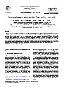
periodic with white noise excitation. The description of the system, the derivation of analytical model, implementation of the technique and validation through a numerical example based on experimental observations (Yim et al, 1993) are presented. SYSTEM CONSIDERED A general single-degree-of-freedom (SDOF), two-point moored structural system restricted to move only in the surge direction is chosen for the study. The model is represented by a submerged rigid body, hydrodynamically damped and an excited nonlinear oscillator (Fig.1). a) wave

N

KEY WORDS: Nonlinear; system identification; multiple-input; single-output; hydrodynamics.

Elastic mooring lines

INTRODUCTION Complex nonlinear responses have been observed in various compliant ocean systems characterized by nonlinear mooring (restoring) force and coupled fluid-structure interaction (exciting) force (e.g. Thompson, 1983; Bishop and Virgin, 1988). Gottlieb (1991) studied the nonlinear behavior of a multi-point symmetric moored structural system under periodic excitation. Lin (1994) extended this analysis by incorporating random noise perturbations. Small body mooring systems are generally solved by a relative-motion Morison formulation (Patel, 1989). It has been observed from the literature that the hydrodynamic drag (Cd) and inertia (Cm) coefficients for sphere are not constants and reasonable estimate could be 0.1 ≤ Cd ≤ 1.0 and 1.0 ≤ Cm ≤ 1.5 respectively (Grace and Casino, 1969; Grace and Zee, 1978). It is important to identify the hydrodynamic coefficients and system parameters to quantitatively examine the nonlinear behavior. Bendat (1990; 1998) has used parallel multiple-input/single-input (MI/SO) procedures for identifying parameters of nonlinear systems. A method for nonlinear system identification to determine amplitude and frequency dependent properties on different types of nonlinear systems such as Duffing, Van der Pol, etc. has been developed by Bendat et al (1992). With the input and output data known, based on multiple input/single output linear analysis of reverse dynamic system, Reverse MI/SO technique identifies the linear and nonlinear system properties. This paper presents the application of the parallel and reverse MI/SO technique on a nonlinear spherical mooring system subjected to

b) waves

z h

x

Fig.1: Definition sketch of the mooring system a) Plan b) Profile. Although the mooring lines are linearly elastic, with large geometric nonlinearity (mooring angles at 90o in this case), the restoring force may become highly nonlinear. Gottlieb (1992) discussed various types of nonlinearities in the restoring force. The elastic mooring cables are

assumed to be taut and the restoring force continuous. The exciting force, considered to be acting at the instantaneous center of the sphere, is represented by relative motion Morison equation (Sarpkaya and Isaacson, 1983). Through an appropriate transformation, the randomness in the wave field is incorporated into the hydrodynamic forcing terms (Shinozuka, 1977).

velocity, u, and acceleration, u& , at the instantaneous center of the sphere can be obtained by using the equations given below: ωd cosh(k ds) cos(k d x − ωd t ) + ζ(t ) sinh(k d h)

(8)

ωd 2 cosh(k ds) sin( k d x − ωd t ) + ζ& ( t ) sinh( k d h )

(9)

u(t) = a d

u& ( t ) = a d

GOVERNING EQUATION

∑ n

ζ( t ) = a s

Assuming that structural damping can be lumped into an equivalent linear structural damping coefficient Cs and the nonlinear restoring force represented by R(x), the governing equation of motion for the mooring system can be written as

j =1

ζ& ( t ) = −a s

∑ N

j =1

(m + m a )&x& + Cs x& + R ( x ) = f ( t )

sinh( k jh )

cos(ω j t + φ j )

ω2 j cosh(k js) sinh( k jh )

sin(ω j t + φ j )

(10)

(11)

(1)

where m = mass of the sphere, ma = added mass, Cs = structural damping coefficient, R(x) = restoring force, f(t) = excitation force, x(t), x& (t), &x& (t) = surge displacement, velocity and acceleration responses, respectively. Using a least square approach, the nonlinear anti-symmetric restoring force can be approximated by a polynomial consisting of odd order terms only. Good agreement between the actual and a two-term polynomial approximation has been demonstrated (Gottlieb, 1992). This polynomial can be written as R ( x ) ≅ k1x + k 3x 3

ω j cosh(k js)

(2)

where h = water depth, s = distance of the center of the sphere from the bottom, and kj = wave number for the white noise signal distributed uniformly between [0,2π]. The exciting force consisting of drag and inertial components acting at the center of the sphere is modeled by one-dimensional Morison equation (Sarpkaya and Isaacson, 1983) given by f ( t ) = ρ∀C m u& ( t ) − m a &x&( t ) +

ρ A pCd (u ( t ) − x& ( t )) u ( t ) − x& ( t ) 2

where ∀=

where k1 and k3 are the linear stiffness coeficient and the nonlinear stiffness coeficient, respectively. EXCITING FORCES Ocean environment including wind waves and current often contain significant component of noise. To examine the nonlinear response of the mooring system from stochastic perspective, randomness in the exciting hydrodynamic force induced by random perturbations in a regular wave profile is included in this study. The wave profile modeled as periodic with white noise is given by

(12)

π 3 D 6

πD 2 4 π 3 m a = D Ca 6 Ap =

(13)

(14)

(15)

where ρ = mass density, D = sphere diameter, Ca = added mass coefficient, Cm = inertia coefficient = Ca+1, and Cd = hydrodynamic drag coefficient. NONLINEAR SYSTEM IDENTIFICATION

η( t ) = a d cos( k d x − ωd t ) + ξ ( t )

(3)

where ad, ωd and kd are the amplitude, frequency and wave number respectively. The disturbance described by ξ(t), represents white noise with zero mean and delta correlation

ξ(t) = 0

(4)

ξ( t )ξ( t ' ) = qδ( t − t ' )

(5)

where q is the noise intensity. The white noise, that can be alternatively idealized as a sum of harmonics of deterministic amplitudes, random frequencies and phase shifts (Shinozuka, 1977), is given by

ξ ( t ) ≅ ξ s ( t ) = a s ∑ cos( ω j t + φ j )

(6)

as = ad ns

(7)

n

j=1

where ns = noise-signal ratio, as = amplitude of the white noise, and ωj, φj’s are the wave frequency and random phase shifts uniformly distributed in [0,2π]. Applying linear wave theory (Chakkrabarti, 1987), the water particle

The generalized schematic model for the nonlinear system under consideration is given in Fig.2. The input wave characteristics, such as η, u, u& , passes through two different systems giving the force output, f(t), which in turn serves as the input to two other systems that yield the displacement output x(t). This is a system identification problem where frequency response functions, such as A1(f), A2(f), etc., can be evaluated by using an equivalent multi-input/single-output linear system identification technique developed by Bendat (1990, 1998). This procedure is applicable to random data irrespective of Gaussian or nonGaussian. Application of this technique is extended to two different areas of parameter identification for the above mooring system, consisting of evaluation of hydrodynamic coefficients and system properties explained in the following paragraphs.

Y1 (f ) 1 = ρCd D 2 U1 (f ) 2

(23)

Y2 (f ) π = ρ D3C m U 2 (f ) 6

(24)

A1 (f ) =

η(t),u(t), u& (t)

x(t)

A 3(f)

A 1(f)

Σ

f(t)

A 2 (f ) =

F1 (f ) = ℑ[f1 ( t )]

Σ

A 2(f) − m a &x& ( t )

-k3 x

(25)

Practical procedures that replace the correlated inputs u1(t) and u2(t) with a new set of uncorrelated inputs and evaluate the frequency response functions are then applied (Bendat, 1998). The frequency response functions A1(f) and A2(f) give the force coefficients Cd and Cm, respectively, as functions of frequency.

3

Nonlinear System Model

Fig. 2: Schematic model for the mooring system Nonlinear Wave Force Model

With the knowledge of wave velocity, acceleration, wave force and system response, the hydrodynamic force coefficients (added mass, added inertia and drag in Eq.(12)) can be evaluated. The methodology used to analyze arbitrary linear systems in parallel for arbitrary nonlinear systems (Bendat, 1990) is extended to the Morison model constructed from the original model (Fig.2). This involves one linear system A1(f) in parallel with a finite-memory nonlinear system g(x, u, t) followed by A2(f) shown in Fig.3 where

g( x , u ) = (u ( t ) − x& ( t )) u ( t ) − x& ( t )

(16)

π f 1 ( t ) = f ( t ) − ρ D 3 C a &x&( t ) 6 π 3 1 2 ρ D C m u& ( t ) + ρC d D (u ( t ) − x& ( t )) u ( t ) − x& ( t ) = f 1 ( t ) 2 6 u 1 ( t ) = u& ( t ) , u 2 (t ) = g(x, u )

(17)

With the simulated force f(t) and the sphere response x(t) as observed data, identification of system parameters for the SDOF nonlinear mooring system model can be obtained by applying the reverse MI/SO technique. Considering the model to be of Duffing type, system diagram formed from the original model (Fig. 2) is given in Fig.4. The general equation for the system model can be written as (m + m a )&x&( t ) + C s x& ( t ) + k 1 x ( t ) + k 3 x 3 ( t ) = f 1 ( t )

A 4 (f)

(26)

x(t)

Σ

f 1 (t)

(18) (19) -k 3 x 3

u1(t) η, u, u&

A1(f)

y1(t)

Fig.4: Nonlinear system model

A2(f)

g(x, u,t) u2(t)

y2(t)

Σ

f1(t)

x(t)

Fourier transforming both sides of Eq.(20) gives the frequency domain relation

where

A 4 (f )F1 (f ) + A 5 (f ) = X (f )

(27)

F1 (f ) = ℑ[f1 ( t )]

(28)

X (f ) = ℑ[x ( t )]

[

A 5 (f ) = ℑ k 3 x ( t )

Fig.3: Nonlinear wave force model The two correlated output records are represented by y1(t) and y2(t). Fourier transforms of both sides of Eq. (18) yield the nonlinear frequency domain formula A 1 (f ) U 1 (f ) + A 2 (f ) U 2 (f ) = F1 (f )

where

U1 (f ) = ℑ[u1 ( t )] ,

U 2 (f ) = ℑ[u 2 ( t )] ,

Y1 (f ) = ℑ[y1 ( t )]

Y2 ( f ) = ℑ[y1 ( t ) ]

(20)

(21) (22)

3

]

(29) (30)

In the absence of nonlinear term x3(t), A4(f) represents the frequency response function of an ideal constant parameter system that relates the displacement output x(t) to the force input f1(t) given by A 4 (f ) =

X (f ) 2 = k 1 [1 − (f f n ) + 2ζ s (f f n )] −1 F1 (f )

(31)

where the natural frequency fn and damping ratio ζs are defined by

(33)

Cs

ςs =

' 2 A 4 ( f r ) = k ⎡ 2ζ s 1 − ζ s ⎤ ⎢⎣ ⎥⎦

(32)

k1 (m + m a )

1 2π

fn =

2 k 1 (m + m a )

2

fr ≈ fn

A 4 (f r ) ≈ 2k 1ζ s '

(39)

(34)

The physical parameters of the mooring system can therefore be estimated as follows (40)

k1 = lim f → 0 A 4' (f ) ’

A4 (f)

(m + m a ) = M ≈ lim f → 0

x(t)

(38)

For lightly damped systems (assumed here), the resonance frequency fr and the minimum value of gain factor can be approximated (Bendat and Piersol, 1993) by

When the nonlinear term is present, A4(f) relates the displacement output x(t) to an effective force fe(t) given by f e (t) = f (t) − k 3 x 3 (t)

ζ s ≤ 0. 5

Σ

C s = 2ζ s

(k 1 (m + m a )) ≈

f1(t)

A 4 ' (f ) (2πf n )

(41)

2

'

A 4 (f n )

(42)

2πf n

The nonlinear impedance function A’5(f) is given by

A5’(f)

g3(x,t)

A 5 (f ) = k 3 '

The linear and nonlinear impedance functions thus give all the system properties.

Fig.5: Reverse dynamic system model Identification of this system requires an iterative approach because of the presence of the feed back term (k3x3). To apply the reverse MI/SO technique, the input/output roles are interchanged. This reverse dynamic system can be viewed as a two-input/singleoutput problem without feedback term as shown in Fig.5. Reverse dynamic inputs x(t) and g3(x,t) = x3(t) may be correlated. The procedures to replace the correlated inputs x(t) and x3(t) with a new set of uncorrelated inputs (Bendat, 1998) are applied to evaluate the frequency response functions. A4’(f), the reciprocal of A4(f) (Eq.31), is defined as the linear impedance function which can also be written as

(

)

A 4 (f ) = [A 4 (f )] = k 1 1 − (f f n ) + 2 jζ s (f f n ) '

−1

2

(34)

The system gain and phase factors of Eq.(34) are given by

(

⎡ ' 2 A 4 (f ) = k 1 ⎢ 1 − (f f n ) ⎣

)

2

2 ⎤ + (2ζ s (f f n )) ⎥ ⎦

⎡ 2ζ s f f n ⎤ φ(f ) = tan ⎢ 2 ⎥ ⎣⎢1 − (f f n ) ⎦⎥ −1

(35) (36)

The minimum gain factor occurs at the resonance frequency fr of the system. By maximizing Eq.(35), it can be shown that for practical structures having damping ratio ζ s 2 ≤ 0.5 , (Clough and Penzien, 1993), and resonance frequency is given by f r = f n 1 − 2ζ s 2

(43)

(37)

NUMERICAL SIMULATION

Parallel and reverse nonlinear system identification methods have been applied to the ocean mooring system described in this document. To demonstrate the applicability of the method, parameters of an existing experimental model (Yim et al, 1993) are chosen that are given in Table 1. The time series and spectrum for numerically simulated periodic with white noise wave and force, Eq.(3) and Eq.(12), with variance same as the experimental inputs is given in Fig.6 and Fig.7. The total time history excitation and response for each simulation is 131,072 samples (8192 seconds), with sub-record lengths of 8192 for the Fourier transforms (512 seconds). Using system parameters in Table 1, the response is obtained by solving the ordinary differential equation using a 4th-order RungeKutta method, Eq.(1), time series and spectrum of which is shown in Fig.8. It can be observed from the figure that response of the sphere is sub-harmonic. The simulated wave, force and response are then used to validate the methodology of system identification. Cd Cm fn ζs k1 k3 M Cs

0.1 1.5 0.252 Hz 0.018 6 N/m 4.3 N/m3 3.29 kg 0.135 kg/s

Table 1: Simulated parameters

and the minimum value of gain factor that occurs at resonance is given by a)

0.80 0.40

Response (m)

Wave (m)

0.60 0.20 0.00 -0.20 -0.40 -0.60 0.00

10.00

20.00

30.00

40.00

50.00

60.00

0.20 0.15 0.10 0.05 0.00 -0.05 -0.10 -0.15 -0.20 -0.25 0.00

10.00

20.00

30.00

40.00

50.00

60.00

Time (second)

Time (second)

b)

b) 1 .0 0 E + 0 1 1 .0 0 E + 0 0

2

Spectrum (m )

2

Spectrum (m )

1.0E+01

1.0E+00

1.0E-01

1 .0 0 E -0 1 1 .0 0 E -0 2 1 .0 0 E -0 3

1.0E-02 0.00

0.50

1.00

1.50

2.00

1 .0 0 E -0 4 0 .0 0

0 .5 0

1 .0 0

1 .5 0

2 .0 0

F req u en c y (H z)

Frequency (H z)

Fig.6: Numerically simulated wave a) Time series b) Spectrum

Fig.8: Numerically simulated response a) Time series b) Spectrum

a)

Force (Newton)

RESULTS AND DISCUSSIONS 12.00 10.00 8.00 6.00 4.00 2.00 0.00 -2.00 -4.00 -6.00 -8.00 0.00

10.00

20.00

30.00

40.00

50.00

60.00

Time (second)

b)

2

Spectrum (Newton )

1.0E+05 1.0E+04 1.0E+03 1.0E+02 1.0E+01 1.0E+00 0.00

0.50

1.00

1.50

2.00

Frequency (H z)

Fig.7: Numerically simulated wave force a) time series b) Spectrum a)

Results are presented for the SDOF nonlinear mooring system. The magnitude of the force coefficients is plotted as a function of normalized frequency in Fig.9a and b. Note that the constant values of drag (Cd) and inertia (Cm) indicate that these coefficients are indeed independent of excitation frequency as assumed. In fact, they match exactly the parameters employed in the simulations, as listed in Table 1. This high degree of accuracy in the parameter estimation is due to the long simulated record available. All randomness was successfully removed by averaging. The corresponding phase values of these coefficients (not shown here) were identically equal to zero as expected, indicating that the constant values of the hydrodynamic coefficients are real and positive. Results of the system model with nonlinear cubic stiffness are presented next. Estimates of the linear impedance function A4’(f), magnitude and phase are given in Fig.10. The magnitude of A4’(f) plotted against frequency normalized with simulated natural frequency, gives all the linear system parameters such as linear stiffness (k1), damping coefficient (Cs), total mass (M) and natural frequency (fn) by using Eq.(40-42). The results match exactly with the simulated parameters given in Table 1. It can be observed from Fig.10a that the minimum of A4’(f ) points at normalized frequency of unity. The phase information given in Fig.10b shows that the phase factor varies from 0o for frequencies less than fn to 180o for frequencies greater than fn and show rapid phase shift at fn. This is common for lightly damped mechanical structures, ζs = 0.018 in this case (Clough and Penzien, 1993). The real part for the nonlinear impedance function, which gives the cubic nonlinear stiffness coefficient used in the simulation, shown in Fig.11. The imaginary part (not shown here) is again observed to be essentially zero. The randomness of the nonlinear stiffness coefficient can be attributed to the fact that magnitude used

200.00

a)

150.00 Angle (Degrees)

for the simulation is small. The trend line shown in Fig.11 matches the simulated magnitude given in Table 1.

Drag Coefficient

1.00

0.10

100.00 50.00 0.00 -50.00 0.00

2.00

4.00

6.00

8.00

10.00

Normalized Frequency 0.01 0.00

2.00

4.00

6.00

8.00

10.00

Fig.10: Linear impedance function a) Magnitude b) Phase

Normalized Frequency

100.00 Nonlinear Impedance

b)

Inertia Coefficient

10.0

10.00

1.00

0.10 0.00

1.0 0.00

4.00

6.00

8.00

8.00

10.00

Fig.11: Nonlinear Impedance function

CONCLUSIONS

a) 1000.00

Linear Impedance Function

6.00

10.00

Fig.9: Force coefficient a) drag b) inertia

100.00

10.00

1.00

2.00

4.00

6.00

Normalized Frequency

b)

4.00

Normalized Frequency

2.00

Normalized Frequency

0.10 0.00

2.00

8.00

10.00

This paper addresses the practical application of a nonlinear system identification technique from the simulated input/output stochastic data in the field of ocean engineering. The identification of hydrodynamic coefficients and structural properties upon knowing the input wave characteristics, wave force and the output system response are the two areas where the methodology of system identification is applied. Different MI/SO linear procedures are applied to a hydrodynamically damped and excited SDOF moored ocean system the equation of motion of which has been defined. A two-input/single-output procedure is directly applied to the nonlinear wave force model and the force coefficients such as drag, Cd, and inertia, Cm, are successfully determined. The identification of hydrodynamic coefficients of the empirically formulated Morison equation from the simulated input/output stochastic data by using this methodology is a valuable contribution towards dynamic wave force analysis. For the nonlinear system model, the reverse MI/SO technique is applied to identify the linear and nonlinear system properties. This method mathematically transforms the single-input/single-output problem to two-input/single-output problem by reversing the roles of input excitation force and response output. The resulting linear and

nonlinear impedance functions correctly identify the properties of the system chosen for the study. The relative contributions from each individual as well as the total terms are quantitatively assessed through coherence functions. ACKNOWLEDGEMENT

The financial support from the United State of Naval Research Grant No. N00014-92-J-1221 is gratefully acknowledged. REFERENCES

Bendat, J.S., Nonlinear System Analysis and Identification from Random Data, John Wiley, New York. 1990. Bendat, J.S., Nonlinear Systems – Techniques and Applcations, John Wiley, New York. 1998. Bendat, J.S., Palo, P.A., and Coppolino, R.N., “A general identification technique for nonlinear differential equations of motion”, Probabilistic Engineering Mechanics, Vol.7, 1992, pp. 4361. Bishop, S.R., and Virgin, L.N., “The Onset of Chaotic Motions of a Moored Semi-Submersible”, Journal of Offshore Mechanics and Arctic Engineering, Vol.110, 1988, pp 205-209. Chakrabarti, S.K., Hydrodynamics of Offshore Structures, Computational Mechanics Publications, London, 1987. Clough, R.W., and Penzien, J., Dynamics of Structures, McGrawHill, 1993.

Gottlieb, O., Nonlinear Oscillations, Bifurcation and Chaos in Ocean Mooring Systems, Ph.D. Dissertation. Oregon State University, 1991. Gottlieb, O., and Yim, S.C.S., “Nonlinear oscillations, bifurcations and chaos in a multi-point mooring system with a geometric nonlinearity”, Applied Ocean Research, Vol.14, 1992, pp.241-257. Grace, R.A., and Casiano, F.M., “Ocean wave forces on a sub surface sphere”, Journal of Waterways and Harbour Division, Vol.95, 1969, pp. 291-312. Grace, R.A., and Zee, G.T.Y., “Further tests on ocean wave forces on sphere”, Journal of Waterway Port Coastal and Ocean Division, Vol.104, 1978, pp.83-88. Lin, H., Stochastic Analysis of a Nonlinear Ocean Structural System, Ph.D. dissertation, Oregon state University, 1994. Patel, M.H., Dynamics of Offshore Structures, Butterworths, London, 1989. Shinozuka, M., “Simulation of Multivariate and Multidimensional Random Processes”, Journal of the Accoustical Society of America, Vol.49, 1977, pp.357-367. Sarpkaya, T., and Isaacson, M., Mechanics of Wave Forces on Offshore Structures, Van Nostrand Reinhold, 1983. Thompson, J.M.T., “Complex Dynamics of Compliant Offshore Structures”, Proceedings of Royal Society London A, Vol.387, 1983, pp.407-427. Yim, S.C.S., Myrum, M.A., Gottileb, O., Lin, H., and Shih,I-M., “Summary and Preliminary Analysis of Nonlinear Oscillations in a Submerged Mooring System Experiment”, Ocean Engineering Report No. OE-93-03, 1993, Oregon State University.