Journal of Electronic Imaging 5(3), 353 – 366 (July 1996).
Nonlinear unsharp masking methods for image contrast enhancement Giovanni Ramponi University of Trieste Department of Electrical Engineering 34127 Trieste, Italy E-mail:
[email protected] Norbert Strobel Sanjit K. Mitra University of California, Santa Barbara Department of Electrical and Computer Engineering Santa Barbara, California 93106 Tian-Hu Yu Chinese University of Hong Kong Department of Information Engineering Shatin-NT, Hong Kong
Abstract. In the unsharp masking approach for image enhancement, a fraction of the highpass filtered version of the image is added to the original image to form the enhanced version. The method is simple, but it suffers from two serious drawbacks. First, it enhances the contrast in the darker areas perceptually much more strongly than that in the lighter areas. Second, it enhances the noise and/or digitization effects, particularly in the darker regions, resulting in visually less pleasing enhanced images. In general, noise can be suppressed with lowpass filters, which are associated with the blurring of the edges. On the other hand, contrast can be enhanced with highpass filters, which are associated with noise amplification. A reasonable solution, therefore, is to use suitable nonlinear filters which combine the features of both highpass and lowpass filters. This paper outlines several new methods of unsharp masking based on the use of such nonlinear filters. Computer simulations have verified the superior results obtained using these filters. In addition, a new measure of contrast enhancement is introduced which quantitatively supports the improvement obtained using the proposed methods. © 1996 SPIE and IS&T.
1 Introduction Image contrast enhancement is concerned with the sharpening of certain image features such as edges or textures, and is employed primarily to improve the visual appearance of an image. Algorithms for contrast enhancement are often employed in an interactive fashion with the choice of the algorithm and the setting of its parameters being dependent on the specific application at hand. Various approaches have been advanced for contrast enhancement. Histogram equalization, a commonly used method, is based on the mapping of input gray levels to
Paper 005NIP received Nov. 13, 1995; accepted for publication May 3, 1996. 1017-9909/96/$6.00 © 1996 SPIE and IS&T.
achieve a nearly uniform output gray level distribution.1,2 However, histogram equalization applied to the entire image has the disadvantage of the attenuation of low contrast in the sparsely populated histogram regions. This problem can be alleviated by employing a local histogram equalization which is of high computational complexity. Another popular approach is unsharp masking ~UM!, in which a fraction of the high-pass filtered version of the image is added to the original signal to form the enhanced image.1,2 The rationale behind this method is to enhance the local change of image intensity which corresponds to the output of the linear highpass filter. However, the method has two serious drawbacks. First, the contrast in the darker areas is enhanced perceptually much more strongly than that in the lighter areas. Second, the method also enhances the noise and/or digitization effects. As a result, in some cases these undesired artifacts become too strong, particularly in the dark regions, resulting in visually less pleasing enhanced images. In order to improve the performance of the UM technique, the use of simple quadratic filters in place of the linear highpass filter has been proposed in Refs. 3, 4. Another modification proposed recently was to place, after the linear highpass filter, a polynomial operator formed by the parallel connection of a linear smoothing filter and a cubic sharpening component.5 In this way the behavior of the filter becomes amplitude-sensitive: for small input amplitude changes, which can be reasonably interpreted as noise, the lowpass linear component dominates and a smoothing effect is obtained; whereas large input variations representing relevant details and captured by the highpass component are further amplified due to the cubic term. Journal of Electronic Imaging / July 1996 / Vol. 5(3) / 353
Ramponi et al.
The use of a quasi-polynomial, direction-sensitive operator has also been recently suggested.6 According to this technique, in the sharpening path a set of parallel branches is used; each branch is formed by the cascade of a linear operator and a nonlinear one, which act orthogonally with respect to each other. In this way, it is possible to sense the presence of correlated image details ~which are enhanced! or noise ~which is attenuated!. To provide uniform contrast enhancement utilizing the unsharp masking techniques, de Vries has proposed a modification based on a logarithmic transformation.7 A third method, called statistical differencing, generates the enhanced image by dividing each pixel value by its standard deviation estimated inside a specified window centered at the pixel.2 Thus, the amplitude of a pixel in the image is increased when it differs significantly from its neighbors, while it is decreased otherwise. A generalization of the statistical difference method includes the contributions of preselected first-order and second-order moments.8 An alternative approach to contrast enhancement is based on modifying the magnitude of the Fourier transform of an image while keeping the phase invariant. In one form of this approach, called a -rooting, the transform magnitude is normalized to the range between 0 and 1 and raised to a power a which is a number between zero and one.9 An inverse transform of the modified spectrum yields the enhanced image. This conceptually simple approach in some cases results in unpleasant enhanced images with two types of artifacts: enhanced noise and replication of sharp edges. By employing a simple polynomial mapping for transform amplitude modification, these artifacts have been reduced resulting in more visually pleasing enhanced images.10 A number of other image enhancement algorithms belong to the class called direct contrast enhancement methods. In these algorithms, a contrast measure is first defined and its original value is modified by a suitably chosen mapping function to develop the enhanced image. Several contrast measures have been proposed by various authors along with different mapping functions.11–14 Of these, in the approach by Yu and Mitra,14 the image contrast is enhanced without increasing the dynamic range of the processed image. In addition, this method yields results matching the characteristics of the human visual system while preserving the shape of the original image histogram. Completely different approaches have also been proposed for contrast enhancement. For example, fuzzy techniques have been devised,15 and they are particularly well suited to deal with image enhancement problems in which objective quality criteria are difficult to establish; they permit dealing with such problems in terms of humanlike reasoning. Of all the proposed contrast enhancement methods, the unsharp masking approach is simplest, both computationally and conceptually. Moreover, it provides a simple interactive feature, which is the amount of the highpass filtered version to be added to the original image. This paper describes a number of modifications to the conventional unsharp masking method by employing nonlinear polynomial filters for feature enhancement. As will be demonstrated later by computer simulations, the proposed modifications yield superior enhanced images both with regard to visual 354 / Journal of Electronic Imaging / July 1996 / Vol. 5(3)
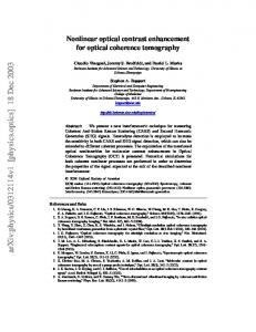
Fig. 1 Conventional unsharp masking technique.
quality and with regard to a new quantitative measure of image enhancement. An outline of the paper is as follows. Section 2 reviews the basic concept of conventional unsharp masking in one dimension based on linear highpass operators and then reviews its modification based on the use of simple quadratic filters. The key properties of these filter types are discussed, and a number of higher-order polynomial operators designed to provide improved enhancement are introduced. These one-dimensional nonlinear operators are extended and generalized to two dimensions in Section 3 for applications in contrast enhancement of images based on the unsharp masking approach. A novel modification to the unsharp masking structure is also advanced here. In addition, specific operators for the enhancement of noisy images are also considered. Section 4 includes detailed computer simulation results obtained using a set of representative nonlinear unsharp masking schemes discussed in the previous sections in order to illustrate the visual quality of the processed images and the improvements achieved with each scheme. It also includes a quantitative comparison of the performances of these schemes using a new figure of merit introduced here. Finally, concluding remarks are included in Section 5. 2
1-D Operators for Unsharp Masking
2.1 Conventional Linear Operators The unsharp masking approach exploits a property of the human visual system called simultaneous contrast. This property leads to the visual phenomenon that the difference in the perceived brightness of neighboring regions depends on the sharpness of the transition; as a result, the image sharpness can be improved by introducing more pronounced changes between the image regions. To this end, a signal proportional to the unsharp version of the image obtained by lowpass filtering is subtracted from the original input. Equivalently, the unsharp masking is implemented by adding a portion of the highpass filtered version of the image back to the image itself. The amount to be added is determined by the user. In one dimension, the unsharp masking operation, shown by the block diagram in Fig. 1, can be represented mathematically as y ~ n ! 5x ~ n ! 1lz ~ n ! ,
~1!
Nonlinear unsharp masking methods
where y(n) and x(n) denote the enhanced signal and the original signal, respectively, z(n) means the sharpening component, and l is a positive constant. The final thresholding operation reduces distortions around high contrast edges without affecting the dynamic range of the original image. A commonly used sharpening component is the one obtained by a linear highpass filter, which can be, for example, the Laplacian operator given by z ~ n ! 52x ~ n ! 2x ~ n21 ! 2x ~ n11 ! .
~2!
Because of the difference operation in Eq. ~2!, the linear highpass filter is, in general, highly sensitive to noise present in the original signal, and the noise is amplified in the process of unsharp masking. 2.2 Quadratic Operators There are also nonlinear operators which behave like linear highpass filters. An example of such an operator is the simple quadratic filter given by z ~ n ! 5x 2 ~ n ! 2x ~ n21 ! x ~ n11 ! .
~3!
This operator, called the Teager’s algorithm, was originally proposed by Kaiser16 to estimate the energy of an oscillating signal. It can be shown that it belongs to a more general class of one-dimensional quadratic filters described by:17
small support sizes, we can approximate sin2(vi) by v 2 i 2 , obtaining a simpler expression for the output z(n): M
z ~ n ! '2A 2 v 2
(
i52M
h ~ i ! x ~ n2i ! x ~ n1i ! ,
z ~ n ! 'A 2 v 2 ,
h ~ i ! 50.
M
z~ n !5
(
i52M
z~ n !'mx 1. They yield a constant output for oscillating inputs with the output being proportional to an input ‘‘energy,’’ defined in the following, if the filter coefficients are appropriately chosen. 2. They respond with a mean-weighted output provided that certain input conditions are met. To validate the first property, consider an input signal of the form ~6!
Substituting Eq. ~6! into Eq. ~4! and performing some manipulations, we arrive at M
(
i52M
h ~ i ! A 2 sin2 ~ v i ! ,
(
i52M
h ~ i !@ x 1 ~ n2i ! 1x 1 ~ n1i !# .
~10!
M
All members of the above class share two main properties:
z ~ n ! 52
h ~ i ! x 1 ~ n2i ! x 1 ~ n1i ! M
1mx
~5!
x ~ n ! 5A sin~ v n ! .
~9!
Due to the assumptions made above, the first ~nonlinear! term can be expected to be much smaller than the second one describing a linear filtering operation. This approximation results in
i5M
(
~8!
which is an estimate of the energy necessary to generate an oscillating input signal.16 Note that Eq. ~7! will generally yield small output values when the filter support is small and the input is slowly varying.17 A small support size can usually be taken for granted as it is necessary to capture local signal properties, which is our objective when using this filter class for unsharp masking. To verify the second property we assume an input signal x(n) which can be modeled by the sum of a local mean m x and a slowly alternating component x 1 (n): x(n)5 m x 1x 1 (n). Substituting this expression in Eq. ~4!, we obtain after some algebra
~4!
where the filter coefficients h(i) satisfy the condition:
i52M
h~ i !i 2.
It should be noted that for the Teager’s algorithm h(0)51 and h(1)5h(21)52 21. As a result, the output reduces to
i5M
z~ n !5
(
i52M
~7!
which is a constant independent of the time index n. For highly oversampled inputs, i.e., for small values of v , and
(
i52M
h ~ i !@ x 1 ~ n2i ! 1x 1 ~ n1i !# .
~11!
In the case of the simple quadratic filter of Eq. ~3!, we arrive at z~ n !'
1 3
@ x ~ n21 ! 1x ~ n ! 1x ~ n11 !#
• @ 2x ~ n ! 2x ~ n11 ! 2x ~ n21 !# ,
~12!
obtained by replacing the local mean m x with the arithmetic mean of neighboring pixels while assuming it to be almost a constant over a small range of time indices. The second factor on the right-hand side of Eq. ~12! can be recognized as the 1-D Laplacian operator verifying the mean-adaptive highpass filtering properties of the Teager operator of Eq. ~3!. The main property of this class of filters, i.e., their mean-weighted highpass response, suggests that they can be useful for unsharp masking of one-dimensional signals. It should also be observed that the mean-weighted response incorporates a property of the human visual system described by Weber’s law.1,2 It states that just-noticeable brightness differences are proportional to average backJournal of Electronic Imaging / July 1996 / Vol. 5(3) / 355
Ramponi et al.
ground brightnesses. Operators belonging to the filter class suggested above indeed yield a smaller output in darker areas and therefore reduce the perceivable noise. Even though the above quadratic operators do take into account Weber’s law, their direct use in unsharp masking may still introduce some visible noise depending on the enhancement factor l chosen. This problem can be alleviated by changing the unsharp masking scheme or by employing higher order nonlinear filters as described in the following. 2.3
Higher Order Polynomial Operators
2.3.1 Basic method The mean-adaptive highpass ~bandpass! filtering property of the simple quadratic filters of Section 2.2 can be exploited to generate higher order polynomial filters that are suitable for contrast enhancement based on the unsharp masking method. For example, the polynomial filter can be formed by simply taking the product of any linear filter with any linear highpass or a bandpass filter. This approach has led to a variety of such higher order polynomial filters for nonlinear unsharp masking.18 Most of these filters provided contrast enhancement with varying degrees of subjective visual quality.
Improved methods In order to improve the performance of the highpass filter we need to condition its operation so as to emphasize only local luminance changes present in the true details of the image, thus avoiding the amplification of noise-induced discontinuities. To achieve this purpose, we can multiply the output of the highpass filter by a control signal obtained from an edge sensor. Both the filter and the edge sensor can be elementary operators, and act on a very small support satisfying two different requirements: the capability of recognizing and enhancing even small details, and simplicity of realization. More precisely, this result is obtained by redefining the sharpening component z(n) in Eq. ~1! as
2.3.2
edges, textures and small details. When the edge sensor has classified the present mask position as belonging to the neighborhood of an edge, the highpass filter is activated and performs the unsharp masking operation. It should be observed from Eq. ~13! that here a cubic operator forms the sharpening signal z(n). As a consequence, z(n) takes very large values in those parts of the image where abrupt and large luminance variations occur. This can create unpleasing effects in the output image, in the form of black or white streaks along some of the object borders. This phenomenon is of very minor relevance in many images, and it can be simply avoided by introducing a saturation effect on the z(n) signal. In all the examples included in this paper, z(n) is clipped so as to take values in the range @ 253104 ,53104 # .
Sharpening low contrast details In some images with low contrast details, the edge sensor output can be too small to permit proper sharpening by the highpass operator. In these cases it is convenient to modify Eq. ~13! as follows:
2.3.3
z ~ n ! 5 $ @ x ~ n21 ! 2x ~ n11 !# 2 1k % 3 @ 2x ~ n ! 2x ~ n21 ! 2x ~ n11 !# .
~14!
A positive value should be chosen for the edge sensor offset factor k in Eq. ~14!; its effect is to give the highpass term an appropriate amplification even when x(n21)'x(n11). Of course, the price to be paid is that noise is proportionally amplified due to the diminished protecting effect of the edge sensor. In fact, the choice of k.0 moves the behavior of the proposed operator towards the one of a conventional linear unsharp masking filter. In principle, if the maximum luminance value of the data is L, a value of k@L 2 @and a suitable choice for l in Eq. ~1!# would lead to an approximation of linear UM.
z ~ n ! 5 @ x ~ n21 ! 2x ~ n11 !# 2 • @ 2x ~ n ! 2x ~ n21 ! 2x ~ n11 !# .
~13!
The first factor on the right-hand side of Eq. ~13! is the edge sensor. It is clear that the output of this factor will be large only if the difference between x(n21) and x(n11) is large enough, while the squaring operation prevents interpreting small luminance variations due to noise as true image details. The edge sensor makes the proposed operator insensitive to the Gaussian-distributed noise which is always present in the data. Indeed, when the mask covers a uniform part of the scene, the @ x(n21)2x(n11) # 2 term has an expected value of zero and is much smaller in practice than the value it takes in the case when the mask overlaps two objects having different luminances. The output of the edge sensor acts as a weight for the signal coming from the second factor in Eq. ~13!, which is a simple linear highpass filter. Thus, the overall correction signal $ z(n) % consists of a highpass version of the original data, with locally adaptive amplification according to the presence of object 356 / Journal of Electronic Imaging / July 1996 / Vol. 5(3)
2.3.4 Taking into account Weber’s law It is possible to tune the proposed operator in order to take into account the human visual system response, and in particular the fact that the just-noticeable difference changes with the average luminance according to Weber’s law.1,2 Merging the proposed operator with the one in Eq. ~12!, we obtain: z ~ n ! 5 $ @ x ~ n21 ! 2x ~ n11 !# 2 1k % @ 2x ~ n ! 2x ~ n21 ! 2x ~ n11 !#
x ~ n21 ! 1x ~ n ! 1x ~ n11 ! . 3
~15!
The local mean estimator @ x(n21)1x(n) 1x(n11)]/3 can also be applied only to the offset term k, in order to avoid an excessive increase of the sensitivity to noise:
Nonlinear unsharp masking methods
z~m,n!52x2~m,n!2x~m12,n ! x ~ m22,n ! 2x ~ m,n12 ! x ~ m,n22 ! .
~19!
2. Type 2B – Q filter: z~m,n!52x2~m,n!2x~m12,n22 ! x ~ m22,n12 ! 2x ~ m12,n12 ! x ~ m22,n22 ! .
~20!
Mitra et al. reported superior sharpening effects when Type 2 – Q operators were used for unsharp masking.4 A more general form of the above type 1 – Q and 2 – Q filters is given by17: M
Fig. 2 Pixels used in (a) type 1A and (b) type 1B filters.
H
z ~ m,n ! 5
M
( (
i52M j52M
h ~ i, j ! x ~ m2i,n2 j ! x ~ m1i,n1 j ! , ~21!
z ~ n ! 5 @ x ~ n21 ! 2x ~ n11 !# 2 x ~ n21 ! 1x ~ n ! 1x ~ n11 ! 1k 3
J
3 @ 2x ~ n ! 2x ~ n21 ! 2x ~ n11 !# . 3
with a coefficient condition M
~16!
2-D Polynomial Operators for Unsharp Masking
3.1 2-D Filter Extensions Extension of the above to 2-D data can be carried out in a variety of ways. The simplest one, which nevertheless yields satisfactory results, is to use separability and to apply the 1-D operator in two orthogonal directions. This method can be used for any one of the 1-D filters described above. Due to the symmetry of all the operators presented in the previous section, there are two possible variations, namely an extension involving horizontal and vertical directions @Fig. 2~a!# or employing diagonal pixel products @Fig. 2~b!#. Yu et al. showed that applying a separable extension to Eq. ~3! results in3:
~17!
~18!
It has been pointed out that both operators yield more pleasing image enhancement results than that obtained using conventional unsharp masking based on linear 2-D highpass filters.3 Moreover, an extension of these so-called type 1 – Q filters led to type 2 – Q nonlinear operators, which can be viewed as local-mean-weighted bandpass filters.4 ~It should be noted that the above filters were called Type 1 and Type 2 filters in Ref. 4.! They are derived from Eqs. ~17! and ~18! by enlarging the support size: 1. Type 2A – Q filter:
h ~ i, j ! 50.
~22!
The above condition has also been used by Ramponi19 as a design rule for 2-D quadratic filters to guarantee preservation of uniform gray levels. Equations ~21! and ~22! comprise a useful nonlinear filter class for image enhancement whose members share the properties of their onedimensional counterparts discussed above. As indicated earlier, we can extend any of the polynomial correction terms in Eq. ~13! to Eq. ~16! by employing a separable 2-D implementation. The simplest operator, which we shall call a type 1A – P filter for future reference, is obtained from Eq. ~13! when extended into horizontal and vertical directions: z ~ m,n ! 5 @ x ~ m21,n ! 2x ~ m11,n !# 2 1 @ x ~ m,n21 ! 2x ~ m,n11 !# 2
2. Type 1B – Q filter: z~m,n!52x2~m,n!2x~m11,n21 ! x ~ m21,n11 ! 2x ~ m11,n11 ! x ~ m21,n21 ! .
( (
i52M j52M
• @ 2x ~ m,n ! 2x ~ m21,n ! 2x ~ m11,n !#
1. Type 1A – Q filter: z~m,n!52x2~m,n!2x~m11,n ! x ~ m21,n ! 2x ~ m,n11 ! x ~ m,n21 ! .
M
• @ 2x ~ m,n ! 2x ~ m,n21 ! 2x ~ m,n11 !# .
~23!
It is a straightforward matter to obtain the type 1B – P 333 operator, which involves the two diagonal directions, and the two corresponding type 2A – P and type 2B – P 535 operators. Similarly, based on Eq. ~14!, we obtain a method which is particularly well suited to images containing both high and low contrast edges. Again using the horizontal and vertical directions, we obtain a type 1A – Pk operator: z ~ m,n ! 5 $ @ x ~ m21,n ! 2x ~ m11,n !# 2 1k % @ 2x ~ m,n ! 2x ~ m21,n ! 2x ~ m11,n !# 1 $ @ x ~ m,n21 ! 2x ~ m,n11 !# 2 1k % @ 2x ~ m,n ! 2x ~ m,n21 ! 2x ~ m,n11 !# ,
~24!
Journal of Electronic Imaging / July 1996 / Vol. 5(3) / 357
Ramponi et al.
while the type 1B – Pk comes from the use of diagonal directions; the type 2A – Pk and type 2B – Pk methods can be defined likewise on a 535 support. Finally, we can take into account the Weber’s law by extending the operator in Eq. ~16! to two dimensions; the resulting type 1A – PW operator takes the form
H
z ~ m,n ! 5 @ x ~ m21,n ! 2x ~ m11,n !# 2 1k
x ~ m21,n ! 1x ~ m,n ! 1x ~ m11,n ! 3
J
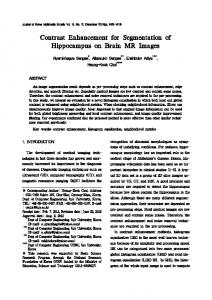
Fig. 3 The proposed modification of the unsharp masking technique.
3 @ 2x ~ m,n ! 2x ~ m21,n ! 2x ~ m11,n !#
H
1 @ x ~ m,n21 ! 2x ~ m,n11 !# 2 1k
x ~ m,n21 ! 1x ~ m,n ! 1x ~ m,n11 ! 3
J
3@ 2x ~ m,n ! 2x ~ m,n21 ! 2x ~ m,n11 !# .
~25!
The remaining three ~type 1B – PW , type 2A – PW , type 2B – P W ,! operators can be defined in the usual way. 3.2 Normalized Nonlinear Unsharp Masking As it will be demonstrated in Section 4, the higher order polynomial operators in Eqs. ~23!–~25! show very low sensitivity to the noise present in the image. An alternative approach to alleviating the noise problem is to modify the unsharp masking structure of Fig. 1 by replacing the sharpening component of Eq. ~1! by an enhancement fraction derived from quadratic filters, which is defined by z ~ m,n ! :5 f
S
D
v~ m,n ! 3x ~ m,n ! max@ u v~ m,n ! u #
~26!
with v (m,n) denoting the output of a quadratic filter. One example of the quadratic filter is the type 1B – Q operator as mentioned in Eq. ~18!. As the filter response v (m,n) in Eq. ~26! can be positive and negative, the function max(uv(m,n)u) is introduced to select the ~overall! maximum absolute value. The ~normalized! quotient v (m,n)/ maxuv(m,n)u is further processed using a sign-preserving power law point transformation f ( • ) to reduce the noise and emphasize significant image details. Applying a signpreserving square function, for example, results in z ~ m,n ! 5sign~ v~ m,n !!
S
v~ m,n ! max@ u v~ m,n ! u #
D
2
3x ~ m,n ! .
Employing this or higher order power functions effectively results in emphasizing strong signal discontinuities as obtained at abrupt edges far beyond a small noise level. Finally, by multiplying the original image x(m,n) with the postprocessed normalized filter output we are able to highlight important edges which, when added back, provide image enhancement. As long as any noise is of small variance, it will be suppressed by this postprocessing step. 358 / Journal of Electronic Imaging / July 1996 / Vol. 5(3)
The block diagram of the normalized unsharp masking technique is shown in Fig. 3. The normalized unsharp masking technique proves to be robust to input images with very different characteristics, i.e, it is not necessary to tune the enhancement factor l precisely to each input image to achieve pleasant enhancement effects.
Specific Operators for Noisy Images Another way of making unsharp masking more robust to noise is to further reduce the noise sensitivity of the higher order polynomial operators presented above. We now define several specifically modified approaches for unsharp masking of noisy images.
3.3
1. Introduce a lowpass linear filter in the direct signal path. Its smoothing effect on the image details will be compensated for by the sharpening path, and the output noise variance will be reduced. 2. Use a more effective edge sensor, such as the Sobel filter.1,2 The final 2-D suboperator in the correction path of the UM scheme will be formed by the product of the outputs of a Sobel filter and a 3 3 3 Laplacian filter. It should be observed that this operator still comes from the 1-D definition of the polynomial filter given in Eq. ~13!, but is obtained using a more sophisticated 2-D extension. 3. Use a combination of the two, i.e. insert the lowpass filter in the direct path of the Sobel–Laplacian operator. Figure 4 shows the block diagram of this algorithm. As the computer simulation will indicate, best results are obtained by resorting to the third approach. Indeed, if e.g. the type 1A – P operator is used in the presence of strong noise, some points in the image appear where the large amplitude of the noise samples activates the edge sensor, creating annoying structures which become particularly visible in the homogeneous areas of the image. The linear filter by itself attenuates the background noise, but is not able to correct for false detections of the polynomial path. In such cases the Sobel filter can be advantageously used at the expense of a slightly larger computational load. Its
Nonlinear unsharp masking methods
y @ m,n # 53x 2 @ m,n # 2 2
1 2
1 2
x @ m11,n11 # x @ m21,n21 #
x @ m11,n21 # x @ m21,n11 #
2x @ m11,n # x @ m21,n # 2x @ m,n11 # x @ m,n21 # . ~27!
Fig. 4 The Sobel–Laplacian technique with the optional lowpass filter.
strength stems from the fact that it combines a highpass and a lowpass action in orthogonal directions, thereby ensuring better noise protection for the sharpener. 4
Computer Simulation Results
4.1 Test Images We now discuss a number of practical examples to illustrate the performance of the proposed operators. Figure 5~a! shows a 2563256 portion of the well-known image ‘‘Lena.’’ The effect of conventional UM is seen in Fig. 5~b! (l50.6); the image is much sharper, but noise is clearly visible in the uniform areas. With a type 1B – Q filter Fig. 5~c! is obtained. Due to the different behavior of this operator in dark and bright areas of the scene, the effects of noise are less visible where the average luminance is low, but are quite apparent in bright areas such as in Lena’s forehead, cheek and shoulder. The scaling factor l used for this test was 256. Finally, Fig. 5~d! shows the effect of the type 1A – P filter, with l50.001. In this image the enhancement of the significant details is very easily perceived, while quantization noise effects are negligible. Very similar results can be obtained from the type 1B – P operator; in this case, a smaller value for l should be used ~say, l50.0007! due to the wider spacing of the pixels involved in the filtering. If the type 1A – Pk operator is used with an offset factor k5400 as defined in Eq. ~24! and l50.00085, we obtain the result shown in Fig. 6. It is seen that some low-contrast details are better enhanced ~observe the longitudinal streaks on the brim of Lena’s hat or the transversal texture of the ribbon in the top left corner!, but at the expense of some noise amplification. The operators which take into account Weber’s law yield the results shown in Fig. 7. Figure 7~a! shows the result of applying a 2-D extension of Eq. ~15! with k50, l50.0003, while Fig. 7~b! comes from the type 1A – PW of Eq. ~25!, k53, l50.00085. The former is noisy and not much sharpened, but the latter is more satisfactory ~observe again the low-contrast details! even if some noise is present. The simulation result obtained using the normalized nonlinear method is shown in Fig. 8. The quadratic filter applied was derived by Thurnhofer,20,21 by optimizing with respect to isotropic edge responses:
The normalized filter output was scaled with a factor l54. The final result shows enhanced edges along the brim of the hat. The eyes are better outlined, and their contrast with the forehead is improved. However, some isolated minute details are also enhanced due to the high local resolution of the filter used. These are perceived as noiselike. In order to further test the noise robustness of the proposed method, the ‘‘Lena’’ original has been corrupted using Gaussian-distributed noise of variance 50. The new test image is reproduced in Fig. 9~a!. If linear UM filtering (l50.55) and the type 1B – Q operator ~scale5256! are applied, the images in Figs. 9~b! and ~c! are respectively obtained; both are well sharpened, but noise is appreciable. The type 1A – P polynomial operator yields Fig. 9~d! (l50.001), which is overall less noisy, but in which some specific large-amplitude noise samples have triggered the sharpening component, thus creating annoying structured disturbance. The insertion of the lowpass filter in the direct signal path slightly improves the performance of the type 1A – P filter @see Fig. 10~a!, l50.0012# and of the normalized unsharp masking technique @see Fig. 10~b!, l57#. While the linear filter suppresses background noise, the enhancement fraction contributes details. However, pixels particularly corrupted by noise cannot be distinguished from details, and some noise is introduced during the unsharp masking process. On the contrary, significantly improved results are obtained using the Sobel-Laplacian operator @Fig. 10~c!, l50.003#: the Sobel filter is able to discern noise from detail with better precision than the elementary edge sensor @ x(n21)2x(n11) # 2 is. As a consequence, the best results are given by the Sobel–Laplacian operator with the lowpass filter in the direct path @Fig. 10~d!, l50.0035#. 4.2 Row-wise Gray Level Plots It is interesting to examine the behavior of the elementary 1-D operators on real world image data and to compare it with the results yielded by other techniques. Figure 11~a! shows the gray level plot of part of a horizontal row of data in the original image ‘‘Lena.’’ It corresponds to the subject’s shoulder, where the luminance smoothly increases from left to right until the steep transition to dark gray when hair is encountered; numerically, this transition starts from gray level 202 at the abscissa n5204 and reaches level 16 at n5210. An ideal sharpening technique should emphasize the change at the shoulder–hair border without amplifying the noise which is recognizable in the smooth part of the plot. Figure 11~b! represents the output of a linear UM operator (l50.8): the desired sharpening effect is present @the gray levels change from 216 (n5204) to 8 (n5211)#, but the most evident effect is noise amplificaJournal of Electronic Imaging / July 1996 / Vol. 5(3) / 359
Ramponi et al.
Fig. 5 Original (a) and processed images: linear UM (b), type 1B – Q (c) and type 1A – P (d) filters.
tion in the smooth region. A different response is obtained by the type 1 – Q filter ~scaling factor 256! and is represented in Fig. 11~c!. As already mentioned, this filter is designed to take into account Weber’s law, and the enhancement effect is stronger when the local luminance is high. Indeed, in the portion of the plot where relatively high gray levels are present ~say above level 128! the response is almost identical to that of the UM operator, with respect to both edge sharpening ~level 216 is reached at n5204! and noise sensitivity; on the contrary, in dark smooth areas we have a reduced noise amplification, and the dark side of the shoulder–hair transition is left almost unchanged ~level 15 at n5211!. If the proposed type 1 – P polynomial filter of Eq. ~14! is used @Fig. 11~d!, l50.0007, k50#, very good results are obtained from both the viewpoint of noise robustness ~the smooth part of the gray level plot is nearly identical to the original one! and that of edge sharpening 360 / Journal of Electronic Imaging / July 1996 / Vol. 5(3)
~level 228 at n5205, level 7 at n5207!. It should be observed that, apart from the overshoot effect which is present at both sides of the edge, the transition itself is steeper ~the bright and dark peaks are located at a distance of only 2 pixels from each other!, as is required of an ideal unsharp masking method.1,2 Finally, if the sharpening of lowcontrast details is desired, a value of k.0 can be chosen, as mentioned above ~type 1 – Pk operator!; the compromise which must be accepted with respect to noise sensitivity is clearly recognizable in Fig. 11~e! ~l50.0007, k5400!. In this case, the behavior with respect to the steep transition is unchanged with respect to the k50 case ~level 228 at n5205, level 7 at n5207!, but a small noise amplification can be seen in the smooth area. The effects of the normalized nonlinear method are recognizable in Fig. 11~f!. As in the ~c! case, edge sharpening took into account Weber’s
Nonlinear unsharp masking methods
Fig. 6 Processed image, type 1A – Pk operator.
law: the bright side of the edge is much more sharpened than the dark side ~the maximum has been saturated to level 255 at n5205; the minimum reached is level 16 at n5210!. 4.3 DV and BV Figures of Merit A quantitative evaluation of the performance of the different methods can be given by defining a suitable figure of merit. It is well known that a quantitative analysis of enhancement is not easy, for at least three reasons: ~i! there is no ideal image to be used as a reference; ~ii! any measure should take into account the complex behavior of human vision, and ~iii! subjective components exist which have not yet been completely understood. In this paper, we simply resort to two figures of merit representing an estimate
Fig. 8 Processed image, normalized nonlinear method.
of the local variance of the original and processed images, performed separately in the detail zones ~detail variance, DV! and in the relatively uniform zones ~background variance, BV! respectively. The estimation technique is described in detail in Ref. 6; it suffices here to observe that we should expect reasonably high values of DV in the enhanced images, while the BV value should remain low in order to indicate small noise amplification. It is clear that the proposed approach does not claim to solve the problem of image quality definition: The figures which are obtained strongly depend on some parameters which need to be set when using this technique. On the other side, once such parameters are set, DV and BV permit one to compare different methods, giving answers which have been shown to agree with human perception in most cases.
Fig. 7 Processed images, Weber’s law correction applied (a) globally and (b) to the offset term k only (type 1A – PW operator).
Journal of Electronic Imaging / July 1996 / Vol. 5(3) / 361
Ramponi et al.
Fig. 9 Noisy original (a) and processed images: linear UM (b), type 1B – Q filter (c), type 1A – P filter (d).
The numerical values in the tables confirm the qualitatively described behavior of the different operators presented in this paper. More precisely, Table 1 permits the comparison of the enhancement mechanisms on the original ~no noise added! ‘‘Lena;’’ in the first row, the DV and BV values for the original data are reported as a reference. It can be seen that the linear UM and the type 1B – Q filter yield approximately equivalent DV, while the latter permits a smaller noise amplification; the polynomial UM achieves the best results with respect to DV and BV. The same filter with offset correction shows a worse BV, as expected, since it amplifies low contrast details in the background portion of the picture. If the polynomial UM is augmented by the local average component, we see that the method in Eq. ~16! performs better than the one in Eq. ~15!, though the best results still are those coming from the simple polynomial UM. On the other hand, it should be observed that 362 / Journal of Electronic Imaging / July 1996 / Vol. 5(3)
DV and BV do not take into consideration the effects of Weber’s law and hence tend to rank some methods inferior which could behave well perceptually. Finally, the normalized nonlinear method yields the results in the last row of Table 1. There a very good BV is achieved at the expense of a smaller sharpening effect. This result reflects the mean-weighted highpass property of the filter used, which results in a reduced filter output for darker image regions. The results obtained from the noisy ‘‘Lena’’ can be quantitatively evaluated using Table 2. As before, the first row shows the DV and BV of the noisy original. These values reflect the added noise, as they are approximately offset by the noise variance. This can be seen when comparing them with their counterparts in the first row of Table 1. We further observe, as before, that the linear UM in the second row and the type 1B – Q operator listed directly be-
Nonlinear unsharp masking methods
Fig. 10 Further results on the noisy original of the previous figure: (a) type 1A – P operator with lowpass filtering in the direct path, (b) normalized nonlinear method with lowpass filtering, (c) Sobel– Laplacian operator, and (d) the same with lowpass filtering.
low show very similar DV; the latter obtains a better BV. From row four we conclude that polynomial UM ranks by far best: it becomes clear that the BV measure is not much penalized by the presence of some structured background noise. The effect of adding a lowpass filter in the direct branch of the Polynomial UM method is apparent in the fifth row: a suitable choice of the parameters permits us to increase DV and reduce BV at the same time, with respect to the previous case. The l of the Sobel–Laplacian operator ~sixth row! can be set so as to yield the same DV as above; the structured noise has almost vanished, but the unstructured is somewhat larger, so that the overall BV is only slightly reduced. A more effective noise control is achieved using the lowpass filter in the direct path as indicated in row seven. The normalized nonlinear method with
lowpass filtering in the direct path finally yields a wellcontrolled BV at the expense of a reduced sharpening effect. 5 Concluding Remarks A wide family of unsharp masking operators based on polynomial filters has been presented in this paper. We have demonstrated by computer simulations that the classical linear UM method can be outperformed from two different points of view, namely the capability of taking into account the human visual system response and, more importantly, the ability to sharpen images even in the presence of noise. A figure of merit has been introduced which evaluates the variance in the smooth and ‘‘active’’ areas of Journal of Electronic Imaging / July 1996 / Vol. 5(3) / 363
Ramponi et al.
Fig. 11 Gray level plots along an image row. Original test image (a) and images after processing using linear UM (b), quadratic UM (c), polynomial UM (d,e), normalized nonlinear UM (f).
the original and processed images. The figure of merit permits us to quantify the results in a way which matches human perception well. It is not possible to state which is the most powerful among the presented methods, because the various operators possess different peculiarities. For example, the normalized nonlinear method can take into account the Weber effect, while the polynomial filters based on edge sensing are more robust to noise. A much larger testbed would be needed, which can not be presented in a reasonably limited 364 / Journal of Electronic Imaging / July 1996 / Vol. 5(3)
space. It is up to the final user to choose and tune the operator according to the specific needs of its application. A possible criticism of the proposed family of operators could concern their heuristic nature. We can cite the fact that image processing is one typical field in which subjectiveness is inherent. Hence, very powerful results have been devised through heuristics: si parva licet componere magnis, i.e. if we are allowed to compare our technique to one of the masterpieces of image processing, the Sobel method for edge extraction is a significant example. On the con-
Nonlinear unsharp masking methods Table 1 DV and BV of the images in Figs. 5–8. Filter Type
Defining Equation
DV
BV
None Linear UM
2-D ext. of Eq. (2)
1161 2637
55 274
Eq. (18) Eq. (23)
2592 2758
186 108 209
Type 1B – Q Type 1A – P Type 1A – Pk
Eq. (24)
2771
Type 1A – PW ,
2-D ext. of Eq. (15)
1796
230
Type 1A – PW ,
Eq. (25) Eqs. (26), (27)
2672 2207
155 89
Normalized nonlinear
Table 2 DV and BV of the images in Figs. 9, 10. Filter Type None (noisy data) Linear UM Type 1B – Q Type 1A – P Type 1A – P1lowpass filter Sobel–Laplacian Sobel–Laplacian1lowpass filter Norm. nonlinear1lowpass filter
DV
BV
1205 2826 2813 2957 3045 3046 3032 1915
104 739 535 308 285 258 211 226
trary, it happens that many well-founded theoretical analyses prove not to be able to be fruitfully translated into practice. These observations are not meant to undervalue the need of a link between the formal analysis of polynomial operators and their design methodologies.
Acknowledgments This work was partially supported by NSF grant No. IRI 94-11330, and in part by a UC Micro grant with matching support from Rockwell International, Digital Instruments, and Tektronix. Further support was received from the European project ESPRIT 20229 Noblesse, and the Italian Ministry of Scientific Research.
References 1. A. K. Jain, Fundamentals of Digital Image Processing, Prentice-Hall, Englewood Cliffs, NJ ~1989!. 2. W. K. Pratt, Digital Image Processing, Wiley, New York ~1991!. 3. T-H. Yu, S. K. Mitra, and J. F. Kaiser, ‘‘A novel nonlinear filter for image enhancement,’’ in Proc. SPIE/SPSE Conf. on Image Processing Algorithms and Techniques II, San Jose, CA, pp. 303–305 ~1991!. 4. S. K. Mitra, H. Li, I. Li and T-H. Yu, ‘‘A new class of nonlinear filters for image enhancement,’’ in Proc. International Conf. on Acoustics, Speech and Signal Processing, Toronto, Canada, pp. 2525–2528 ~Apr. 1991!. 5. G. Ramponi and G. L. Sicuranza, ‘‘Image sharpening using a polynomial operator,’’ in Proc. European Conf. on Circuit Theory and Design, ECCTD-93, Davos, Switzerland, pp. 1431–1436 ~Aug.–Sep. 1993!. 6. A. Vanzo, G. Ramponi, and G. L. Sicuranza, ‘‘An image enhancement technique using polynomial filters,’’ in Proc. First IEEE International Conf. on Image Processing, Austin, TX, pp. 477–481 ~Nov. 1994!. 7. F. P. Ph. de Vries, ‘‘Automatic, adaptive, brightness independent contrast enhancement,’’ Signal Process. 21, 169–182 ~Oct. 1990!.
8. R. H. Wallis, ‘‘An approach for the space variant restoration and enhancement of images,’’ in Proc. Symp. on Current Mathematical Problems in Image Science, Monterey, CA ~Nov. 1976!. 9. H. C. Andrews, A. G. Teschler, and R. P. Kruger, ‘‘Image processing by digital computer,’’ IEEE Spectrum 9, 20–32 ~July 1972!. 10. S. K. Mitra and T-H. Yu, ‘‘Transform amplitude sharpening: a new method of image enhancement,’’ Comput. Vision, Graphics Image Process. 40, 205–218 ~1987!. 11. R. Gordon and R. M. Rangayyan, ‘‘Feature enhancement of film mammograms using fixed and adaptive neighborhoods,’’ Appl. Opt. 23~4!, 560–564 ~Feb. 1984!. 12. A. P. Dhawan, G. Buelloni, and R. Gordon, ‘‘Enhancement of mammographic features by optimal adaptive neighborhood image processing,’’ IEEE Trans. Med. Imaging MI-5, 8–15 ~Mar. 1986!. 13. A. Beghdadi and A. L. Negrate, ‘‘Contrast enhancement based on local detection of edges,’’ Comput. Graphics Image Process. 46, 162–174 ~1989!. 14. T.-H. Yu and S.K. Mitra, ‘‘A histogram-shape preserving algorithm for image enhancement,’’ in Proc. IEEE International Symp. on Circuits and Systems, Chicago, pp. 407–411 ~May 1993!. 15. F. Russo and G. Ramponi, ‘‘A fuzzy operator for the enhancement of blurred and noisy images,’’ IEEE Trans. Image Process. 4~8!, 1169– 1174 ~Aug. 1995!. 16. J. F. Kaiser, ‘‘On a simple algorithm to calculate the ‘energy’ of a signal,’’ in Proc. IEEE International Conf. on Acoustics, Speech and Signal Processing, Albuquerque, NM, No. 1, pp. 381–384 ~May 1990!. 17. N. Strobel, Quadratic Filters for Image Contrast Enhancement, Dept. of Electrical and Computer Engineering, Univ. of California, Santa Barbara ~June 1994!. 18. T.-H. Yu and S. K. Mitra, ‘‘Unsharp masking with nonlinear filters,’’ in Proc. EURASIP Seventh European Signal Processing Conf., EUSIPCO-94, Edinburgh, Scotland, pp. 1485–1488 ~Sep. 1994!. 19. G. F. Ramponi, ‘‘Bi-impulse design of isotropic quadratic filters,’’ Proc. IEEE 1, 665–677 ~Apr. 1990!. 20. S. Thurnhofer, ‘‘Quadratic Volterra filters for edge enhancement and their application in image processing,’’ PhD Thesis, Dept. of Electrical and Computer Engineering, Univ. of California, Santa Barbara, ~Dec. 1994!. 21. S. Thurnhofer and S. K. Mitra, ‘‘A general framework for quadratic Volterra filters for edge enhancement,’’ IEEE Trans. Image Process. 5~6!, 950–963 ~June 1996!.
Giovanni Ramponi graduated in electronic engineering (summa cum laude) from the University of Trieste, Italy, in 1981. In 1983 he joined the Department of Electronics of the University of Trieste as a research engineer; in 1986 he was appointed senior research engineer. Since 1992, he has been an associate professor of applied electronics. Prof. Ramponi has contributed to several undergraduate and graduate courses on analog and digital electronics and on digital signal processing. His research interests include nonlinear digital signal processing, enhancement and feature extraction in images and image sequences, and image compression. He has published more than 60 papers in international journals and conference proceedings.
Norbert Strobel received the BS degree from the University of ErlangenNuremberg, Germany, in 1991, and the MS degree from the University of California, Santa Barbara, in 1994, where he is now working towards his PhD at the Image Processing Laboratory. His research interests include digital signal and image processing, computer vision, and image databases.
Journal of Electronic Imaging / July 1996 / Vol. 5(3) / 365
Ramponi et al. Sanjit K. Mitra received the PhD degree in electrical engineering from the University of California, Berkeley, in 1962. He has been a professor of electrical and computer engineering at the University of California, Santa Barbara, since 1977, and served as the chairman of the department from July 1979 to June 1982. Dr. Mitra served as the President of the IEEE Circuits and Systems Society in 1986, and has served IEEE in various other capacities. He is a fellow of the IEEE, AAAS, and SPIE. He received the F. E. Terman Award and the ATT Foundation Award of the American Society for Engineering Education in 1973 and 1985, respectively. He received the IEEE Circuits and Systems Society Education Award in 1989 and the IEEE Signal Processing Society Technical Achievement Award in 1995. He was awarded an Honorary Doctorate of Technology degree from the Tampere University of Technology, Tampere, Finland in May 1987.
366 / Journal of Electronic Imaging / July 1996 / Vol. 5(3)
Tian-Hu Yu graduated from the Harbin Institute of Military Engineering, Harbin, China, in 1968. He joined the faculty of the Dalian Maritime University, Dalian, China, in 1977. He was a visiting scholar with Signal and Image Processing Laboratory, University of California, Santa Barbara, from 1983 to 1986 and from 1988 to 1990. He received his MS and PhD degrees in signal processing from the University of California, Santa Barbara, in 1990 and 1992, respectively, and then he was a postdoctoral researcher there. Since August 1993, he has been with the Department of Information Engineering, the Chinese University of Hong Kong, Hong Kong. His research interests include digital signal processing, image processing, and data compression.