Nov 21, 2013 - well as real networks; in particular, we investigate the support for ..... as a single between-block link probability (complete pooling) as in [15].
arXiv:1311.1033v2 [stat.ML] 21 Nov 2013
Nonparametric Bayesian models of hierarchical structure in complex networks Mikkel N. Schmidt, Tue Herlau, and Morten Mørup 15 September 2012 Abstract Analyzing and understanding the structure of complex relational data is important in many applications including analysis of the connectivity in the human brain. Such networks can have prominent patterns on different scales, calling for a hierarchically structured model. We propose two non-parametric Bayesian hierarchical network models based on Gibbs fragmentation tree priors, and demonstrate their ability to capture nested patterns in simulated networks. On real networks we demonstrate detection of hierarchical structure and show predictive performance on par with the state of the art. We envision that our methods can be employed in exploratory analysis of large scale complex networks for example to model human brain connectivity.
1
Introduction
Complex networks are an integral part of all natural and man made systems. Our cells signal to each other, we interact in social circles, our cities are connected by transportation, water and power systems and our computers are linked through the Internet. Modeling and understanding these network structures have become an important endeavor in order to comprehend and predict the behavior of these many systems. A central organizational principle is that entities are hierarchically1 organized and that these hierarchical structures plays an important role in accounting for the patterns of connectivity in these systems [9,22,28,30,32,33]. A common notion in modeling complex network is the idea of communities: Groups of nodes that are more densely connected internally than externally. This notion has led to models of networks as collections of groups of nodes that determine how edges are formed [11, 25]. For instance, people in a social network may be grouped according to family, workplaces, schools, or entire countries, and it is assumed these groups determine the formation of social relations. In many 1 In this work we define a hierarchy to denote a decomposition of a complex relational system into nested sets of subsystem rather than as a formal organization of successive sets of subordinates [33].
1
complex systems communities do not exist only at a single scale but can further be partitioned into submodules and sub-submodules, i.e., as parts within parts [22, 33]. For instance, are the communities in a network of schoolchildren in a city best described by schools or school classes? How about social cliques within classes or year groups of classes? It seems that different answers are relevant in different contexts influencing the scale on which the network should be analyzed; but discovering the hierarchical structure governing such relationships in a network would tell us more than any particular choice of resolution. Previous research on discovering hierarchical structure in networks has primarily focussed on binary trees [2, 8, 9, 27, 29–31]. Given a set of nodes and a matrix of affinities between them, a commonly used tool to uncover their organization is hierarchical clustering using either agglomerative [2, 29] or divisive approaches [8, 27]. These traditional hierarchical clustering approaches, however, have the following three major drawbacks [32]: 1. They are local in their objective function and do not form a well defined global objective. 2. The number of partitions is not well defined and various heuristics are commonly invoked to determine this number. 3. The output is always a binary hierarchical tree, regardless of the underlying true organization. Addressing the first two drawbacks, a number of non-parametric Bayesian models have been proposed: Roy et al. [30] and Clauset et al. [9] have studied Bayesian generative models for binary hierarchical structure in networks, assuming a uniform prior over binary trees, and Roy and Teh have proposed the Mondrian Process [31] in which groups are formed by recursive axis-aligned bisections. Addressing the third drawback, Herlau et al. [14] have proposed using a uniform prior over multifurcating trees with leafs terminating at groups of network nodes, and Knowles and Ghahramani [19] have mentioned the applicability of their multifurcating Pitman-Yor Diffusion tree as a prior for learning structure in relational data. In this work we propose two non-parametric Bayesian hierarchical network models based on multifurcating Gibbs fragmentation trees [21]. We leverage Bayesian nonparametrics to devise models that: • Are generative. This allows us to simulate networks from the model, e.g., for use in model checking, and gives a principled approach to handling missing data. • Capture structure at multiple scales. The models simultaneously learns about structures from macro scale involving the whole network to micro scale involving only a few nodes. • Can infer whether or not hierarchical structure is present. If there is no support for a hierarchy the models can reduce to a non-hierarchical structure. 2
• Are consistent and infinitely exchangable. The models are extendable to an infinite sequence of networks of increasing size, allowing them to increase and adapt their structure to accomodate new data. The paper is structured as follows. In section 2 we review the Gibbs fragmentation tree process [21] and describe our models for hierarchical structure in network data. In section 3 we analyze the hierarchical structure in simulated as well as real networks; in particular, we investigate the support for hierarchical structure in structural whole brain connectivity networks derived from diffusion spectrum imaging based on the data provided Hagmann et al. [13]. In section 4 we present our conclusions and avenues of further research.
2
Models and methods
2.1
Fragmentation processes and trees
Following the presentation in [21], we review the multifurcating Gibbs fragmentation tree process. The end result is a projective family of exchangeable distributions over rooted multifurcating trees with n leafs. A rooted multifurcating tree can be represented by a fragmentation of the set of leafs. Let B be the set of leafs and n = |B| the total number of leafs. Recall that a partition πB of B is a set of 2 or more non-empty disjoint subsets of B, πB = {B1 , B2 , . . . , Bk }, such that the union is B. In the following we denote the size of these subsets by ni = |Bi |. A fragmentation TB of a set B is a collection of non-empty subsets of B defined recursively such that the set of all nodes is a member, B ∈ TB ; each member of the partition πB is a member, B1 ∈ TB , . . . , Bk ∈ TB ; each member of partitions of these subsets are members, and so on until we reach the singletons. Recursively we may write [21] � {B}, |B| = 1, TB = (1) {B} ∪ TB1 ∪ · · · ∪ TBk , |B| ≥ 2. For example, the tree in Figure 3 which has leafs B = {1, � 2, 3} is represented by the fragmentation TB = {1, 2, 3}, {1, 2}, {1}, {2}, {3} . Uniquely associated with the fragmentation is a multifurcating tree where each element in TB above serves as a node: B is the root node, and the singletons are the leafs. To emphasize this connection, TB is called a fragmentation tree [21]. The collection of all fragmentation trees for a set B is denoted by TB . Let A ⊂ B be a nonempty proper subset of the leaf nodes. The restriction of TB to A is defined as “the fragmentation tree whose root is A, whose leaves are the singleton subsets of A and whose tree structure is defined by restriction of TB .” [21]. This is also called the projection of TB onto A and denoted by TB,A . A random fragmentation model [21] assigns a probability to each tree TB ∈ TB for each finite subset B of N. The model is said to be: • Exchangeable if the distribution of TB is invariant to permutations on B, i.e., the distribution does not depend on the labelling of the leaf nodes. 3
Figure 1: A Markovian consistent splitting rule satisfies the condition that the probability of a partition is equal to the sum of the probabilities of all configurations where a single extra node is added. • Markovian if, for a given πB = {B1 , B2 , . . . , Bk }, each of the k restricted trees TBi ,B are independently distributed as TBi . • Consistent if, for all nonempty A ⊂ B, the projection of TB onto A is distributed like TA . The starting point for constructing a random fragmentation model is a distribution over partitions of B. By exchangeability this distribution must be a symmetric function depending only on the size of each subset, � q(πB ) = q n1 , . . . , nk , (2) where q is called the splitting rule. Abusing notation, we write the splitting rule as a function of a partition or equivalently as a function of the sizes of the subsets in the partition. Requiring Markovian consistency places a further constraint on the splitting rule [21] (see Figure 1), � � q n1 , . . . , n k = q n1 , . . . , n k , 1 + � � q n1 + 1, . . . , nk + · · · + q n1 , . . . , nk + 1 + � � q 1, n1 + · · · + nk q n1 , . . . , nk . (3) McCullagh et al. [21] show that under the further condition that the splitting rule is of Gibbs form, k
q n1 , . . . , n k
�
a(k) Y � w(ni ), = c n i=1
(4)
where w(·) ≥ 0 and a(·) ≥ 0 are some sequences of weights and c(·) is a normalization constant. Specifically the only admissible splitting rule is given by2 q(n1 , . . . , nk ) =
β (k) ) (−1)k (α
k Y
β β (n) − α (−α)(n)
i=1
(−α)(ni ) ,
(5)
where x(y) = x(x + 1) · · · (x + y − 1) = Γ(x+y) Γ(x) denotes the rising factorial. The splitting rule has two parameters, α ≥ 0 and β ≥ −α. To simplify the notation in the following we define q(0) = q(1) = 1. 2 McCullagh
et al. [21] do not give an explicit formula for the normalization constant.
4
Figure 2: Multifurcating trees generated from the two-parameter Gibbs fragmentation tree process. The parameters govern the distribution of the degree of the internal nodes in the tree. The trees shown correspond to α ∈ {0.1, 0.5, 1} and β + α ∈ {0.1, 1, 10}. By the Markovian property the distribution over fragmentations can then be characterized as a recursive product of these splitting rules, one for each set in the fragmentation or equivalently for each node in the tree. This gives rise to the following representation of all exchangeable, Markovian, consistent, Gibbs fragmentation processes, Y p(TB ) = q(πA ), (6) A∈TB
where q(·) is given by Eq. (5) and πA denotes the children of node A in TB . To illustrate how the properties of the Gibbs fragmentation tree distribution is governed by the two parameters α and β we have generated a few trees from the distribution, varying the parameters within their range (see Figure 2).
2.2
Relation to the nested CRP
The Gibbs fragmentation tree is closely related to the two-parameter version of the Chinese restaurant process (CRP) [3]. The CRP is a partition-valued discrete stochastic process: For n = 1 element, the CRP assigns probability one to the trivial partition. As n increases, element number n + 1 is added to an i −α or added to the existing set of elements in the partition with probability nn+β partition as a new singleton set with probability β+kα n+β . Taking the product of n such terms yields the expression for the probability assigned to a given partition πB , � k β Γ(β)αk Γ α + k Y Γ(ni − α) p(πB ) = . (7) � β Γ(1 − α) Γ(β + n)Γ α i=1 5
As the number of elements goes to infinity, the CRP defines a distribution over partitions of a countably infinite set. Now, consider a set of nested Chinese restaurant processes as proposed by Blei et al. [5,6]: First, the set B is partitioned into πB = {B1 , . . . , Bk } according to a CRP. Next, each subset Bi is partitioned again according to a CRP with the same parameters, and the process is continued recursively ad infinitum (see Figure 3). This nested CRP thus defines “a probability distribution on infinitely deep, infinitely branching trees.” [5]. Blei et al. use this nested CRP as a prior distribution in a Bayesian non-parametric model of document collections by assigning parameters to each node in the tree and associating documents with paths through the tree. In the nested CRP, each element traces an infinite path through the tree. When a finite number of elements n is considered, they trace a tree of finite width but infinite depth. In the terminology of the random fragmentation model, the nested CRP model corresponds to a fragmentation tree using a CRP as a splitting rule. The key difference between the Gibbs fragmentation trees and the nested CRP is that the CRP splitting rule allows fragmenting into the trivial partition, i.e., it allows nodes with a single child whereas the Gibbs fragmentation tree allways has at least two children. Instead of working directly with this infinitely deep tree, we can consider the equivalence class of trees with the same branching structure by marginalizing over the internal nodes that do not branch out, yielding a tree of finite depth. The distribution for this equivalence class can be arrived at by marginalizing over the number of consecutive trivial partitions that occurs before the first “real” split. According to the CRP in Eq. (7), the trivial partition has probability � β + 1 Γ(n − α) Γ(β)αΓ α . (8) p0 ≡ p (πB = {B}) = � β Γ(1 − α) Γ(β + n)Γ α We wish to marginalize over seeing zero, one, two, etc. trivial partitions before the first split. To compute this marginalization, the CRP distribution must be multiplied by 1 + p0 + p20 + · · ·
=
1 1 − p0
=
β (n) , (9) β β (n) + α (−α)(n)
where we have inserted Eq. (8) and used the geometric series formula to compute the infinite sum. Multiplying Eq. (9) by the CRP in Eq. (7) yields exactly the splitting rule of McCullagh et al. in Eq. (5) establishing the relation between the Gibbs fragmentation tree and the nested CRP.
2.3
Tree-structured network models
We now turn to applying the Gibbs fragmentation process as a prior in a Bayesian model of hierarchical structure in complex networks. To simplify the presentation we focus on simple graphs but note that the main ideas can be 6
Figure 3: Illustration of the relation between the nested Chinese restaurant process (CRP) and its finite representation as a Gibbs fragmentation tree. In the nested CRP, each internal node in the tree splits into an infinite number of subtrees. Each element associated with the tree traces a infinite path starting at the root. In the illustration three elements are associated with the tree; thus, the hierarchical structure relating the observables (which is what we are ultimately interested in learning) can be represented by a Gibbs fragmentation tree of finite size. As an example, in the finite representation the root node (labeled “123”) corresponds to the first common ancestral node of all observables as well as the parents and grandparents etc. of that node all the way to the root of the tree. extended to more intricate relational data such as weighted and directed graphs etc. A simple graph with n nodes can be represented by a symmetric binary adjacency matrix A with element ai,j = 1 if there is a link between node i and j. First, consider a model in which each possible link ai,j is generated independently from a Bernoulli distribution (a biased coin flip) with probability θi,j . Since each possible link has its own parameter, no information is shared in the model between different nodes and links and the model will not be able to generalize. Combining information between network nodes is necessary, for example by pooling the parameters for blocks of similar nodes. The particular way in which these parameters are shared is the key difference between the models we discuss here. In the stochastic blockmodel [16, 34] network nodes are clustered into blocks which share their probabilities of linking within and between blocks. The infinite relational model (IRM) [18, 37] is a nonparametric Bayesian extension of the stochastic blockmodel based on a CRP distribution over block structures. We consider the IRM model the state of the art in Bayesian modeling of large scale complex networks. The link probabilities between the blocks in these models can either be individual for each pair of blocks (unpooled) as in the IRM model or be completely shared as a single between-block link probability (complete pooling) as in [15]. Furthermore the model can specify that blocks have more internal than exter-
7
nal links leading to an interpretation of the blocks as communities of highly interconnected nodes [26]. The hierarchically structured models of complex networks proposed here correspond to nested stochastic blockmodels in which each block is recursively modelled by a stochastic blockmodel, and we use the Gibbs fragmentation tree process as a prior over the nested block structure. As in the stochastic blockmodel, links between blocks can be pooled or not, leading to models with different characteristics. Figure 4 illustrates these different approaches to pooling parameters in block structured network models, and Figure 5 illustrates a network that can be well characterized by a hierarchical block structure. Let A denote the observed network and let T denote a fragmentation of the network nodes. The following general outline of a probabilistic generative process can be used to characterize a complex network with a hierarchical cluster structure. 1. Generate a rooted tree T where the leaf nodes corresponds to the vertices in the complex network, T ∼ p(T |τ ). (10) Each internal node in the tree corresponds to a cluster of network vertices. 2. For each internal node in the tree, generate parameters θ that govern the probabilities of edges between vertices in each of its children, θ ∼ p(θ|T, ρ).
(11)
3. For each pair of vertices in the network, generate an edge with probability governed by the parameters located at their common ancestral node in the tree, A ∼ p(A|θ, T, ξ). (12) Several existing hierarchical network models [9, 14, 30] are special cases of this approach with different choices for the distributions of T , θ, and A. Inference in these models entails computing the posterior distribution over the latent tree structure, Z p(A|θ, T )p(θ|T )p(T ) dθ. (13) p(T |A) = p(A) In the following, we consider two hierarchical block models: An unpooled and a pooled model (see Figure 4). As a distribution over trees we use the Gibbs fragmentation model in Eq. (6). The likelihood for both models can be written as a product over all internal nodes in the tree, Y p(A|θ, T ) = fB (A, θ B , B). (14) B∈T |B|≥2
8
Figure 4: Illustration of different approaches to modelling (hierarchical) group structure in complex networks. The figures shows matrices of probabilities of links between groups in a network with five groups (darker color indicates higher link probability). Groups of nodes can be allowed to link to other groups with independent probabilities (denoted blocks), or restricted to have higher probability of links within than between groups (denoted communities). Furthermore, between-group link probabilities can be independent (unpooled) or shared (pooled) amongst all groups at each level of the hierarchy.
9
Figure 5: Simulated example of a complex network with hierarchical group structure. The network has five clusters; however, three of these (top and left) are more connected to each other than to the remaining two clusters, forming a super cluster. The goal of this work is to automatically detect such hierarchical structure and learn from data the number of clusters, their hierarchical organization, as well as the depth of the hierarchy.
10
Assume that the set B according to T fragments into the partition {B1 , B2 , . . . , Bk } and `, m denote indices of each fragment. The likelihood then has the following form, Y Y Bernoulli(θB,`,m ), (15) fB (A, θ B , B) = B` ∈B i∈B` Bm ∈B j∈Bm l