Nonparametric Estimation of Raindrop Size Distributions from Dual ...

1008

JOURNAL OF ATMOSPHERIC AND OCEANIC TECHNOLOGY

VOLUME 24

Nonparametric Estimation of Raindrop Size Distributions from Dual-Polarization Radar Spectral Observations DMITRI N. MOISSEEV

AND

V. CHANDRASEKAR

Colorado State University, Fort Collins, Colorado (Manuscript received 25 April 2006, in final form 13 September 2006) ABSTRACT This paper presents a method to retrieve raindrop size distributions (DSD) from slant profile dualpolarization Doppler spectra observations. It is shown that using radar measurements taken at a high elevation angle raindrop size distributions can be retrieved without making an assumption on the form of a DSD. In this paper it is shown that drop size distributions can be retrieved from Doppler power spectra by compensating for the effect of spectrum broadening and mean velocity shift. To accomplish that, spectrum deconvolution is used where the spectral broadening kernel width and wind velocity are estimated from spectral differential reflectivity measurements. Since convolution kernel is estimated from dualpolarization Doppler spectra observations and does not require observation of a clear-air signal, this method can be used by most radars capable of dual-polarization spectra measurements. To validate the technique, sensitivity of this method to the underlying assumptions and calibration errors is evaluated on realistic simulations of radar observations. Furthermore, performance of the method is illustrated on Colorado State University–University of Chicago–Illinois State Water Survey radar (CSU– CHILL) measurements of stratiform precipitation.

1. Introduction Rainfall radar observations depend on underlying raindrop size distributions. Since rain-rate retrieval from radar measurements is a problem of current interest there is a great importance in independent measurements of naturally occurring drop size distributions. Often in situ measurements of raindrop size distributions are performed using disdrometers (Bringi et al. 2003). Despite wide acceptance of these measurements as a ground truth, the small sampling volume limits accuracy of these measurements (Ulbrich and Atlas 1998). Jameson and Kostinski (2001) have argued that raindrop size distributions (DSDs) are sampling volume dependent and that observed raindrop size distributions should be compared only if observed at comparable scales. The relation between raindrop fall velocity and equivolumetric diameter (Atlas et al. 1973) brought a possibility of converting vertical Doppler radar mea-

Corresponding author address: Dmitri N. Moisseev, Department of Electrical and Computer Engineering, Colorado State University, Fort Collins, CO 80523. E-mail: [email protected] DOI: 10.1175/JTECH2024.1 © 2007 American Meteorological Society

JTECH2024

surements to raindrop size distributions. This approach allows for increasing an observation volume to radar resolution volume scales. Since Doppler power spectra of rainfall are influenced by turbulence and wind, the DSD retrieval procedure is not straightforward. Atlas et al. (1973) have shown that if effects of turbulence and wind are not accounted for, the retrieved DSD would be largely erroneous. Parameterization of raindrop size distributions (Ulbrich 1983; Willis 1984) allowed for using optimization approach to find parameters of DSD. Hauser and Amayenc (1981) have shown that under certain assumptions intercept parameter and median volume diameter of exponential DSD can be retrieved from Doppler spectra observations. The proposed method, however, did not include effects of turbulence and wind. Williams (2002) have extended this approach by including spectrum broadening and wind effects and assuming that raindrop size distributions follow a gamma functional form that allowed DSD parameters retrieval from profiler measurements. A similar procedure was also implemented by Moisseev et al. (2006) for slant profile radar measurements. Russchenberg (1993) used spectral moments to retrieve parameters of a drop size distribution. The main limitation of these

JUNE 2007

1009

MOISSEEV AND CHANDRASEKAR

methods, though, is dependence on one or another functional form of the DSD. The sensitivity of VHF wind profilers to both clearair and precipitation signals has brought another possibility for estimating drop size distributions. Gossard (1988) and Rajopadhyaya et al. (1993) have proposed to use deconvolution techniques to remove the effect of turbulence and wind from Doppler spectra measurements. In this procedure the broadening kernel width and wind velocity were obtained from clear-air measurements. The drawback of this approach is that clearair spectrum has a finite length and often contaminates measurements of the precipitation spectrum. To mitigate this problem Currier et al. (1992) has proposed the use of dual-frequency profiler retrieval, by combining clear-air measurements from a VHF profiler with precipitation observations taken by a UHF profiler. May et al. (2001, 2002) and May and Keenan (2005) have shown that the dual-frequency approach can successfully be applied in variety of measurement conditions. Introduction of dual-polarization radar measurements (Seliga and Bringi 1976, 1978) has brought a new possibility to radar rainfall observations. Dualpolarization rain-rate retrieval techniques have been demonstrated to be more accurate than reflectivitybased ones. The dual-polarization methods rely on changes of raindrop shapes with diameter. Generally, raindrop shape is approximated by a spheroid with axis ratio being a function of raindrop diameter. There are a number of theoretical and experimental studies on raindrop shapes (Pruppacher and Beard 1970; Beard and Chuang 1987; Andsager et al. 1999; Thurai et al. 2006). Kezys et al. (1993) and Unal et al. (1998) have demonstrated measurements of the spectral differential reflectivity in precipitation. Recently Moisseev et al. (2006), Spek et al. (2005), and Unal et al. (2001) have combined dual-polarization and Doppler observations to retrieve microphysical properties of precipitation. Wilson et al. (1997) have also shown that a combination of dual-polarization and Doppler observations can be used to constrain the shape parameter of a gamma DSD. Based on simulations, Moisseev et al. (2006) have shown that an optimum combination of Doppler and dual-polarization measurements can be achieved if observations are taken at elevation angles ranging between 30° and 60°. Furthermore, it was shown that spectral differential reflectivity measurements can be related to raindrop shapes and air motion. In this work we propose to use spectral differential reflectivity observations to estimate a spectrum broadening kernel width and wind velocity. Then by applying this information one can remove influence of spectral broaden-

ing and wind from a Doppler power spectrum and therefore retrieve a raindrop size distribution. This paper is structured as follows. In section 2, dualpolarization spectral observations are introduced. Furthermore, in this section the connection between spectral differential reflectivity and precipitation microphysical properties is described. The DSD retrieval method is outlined in section 3. In section 4 a detailed error analysis of the proposed method is given. Implementation of the method to the Colorado State University–University of Chicago–Illinois State Water Survey radar (CSU–CHILL) data is shown in section 5. Finally discussion and conclusions are given in sections 6 and 7.

2. Differential reflectivity spectrum Doppler power spectra of precipitation echoes can be written as follows (Wakasugi et al. 1986): Sobs共␷兲 ⫽ Spr共␷兲*Sb共␷ ⫺ ␷0兲,

共1兲

where Spr(␷) is the power spectrum due to scattering from hydrometeors, Sb(␷) is the spectrum broadening kernel, the asterisk (*) denotes circular convolution, and ␷0 is the wind radial velocity component. The spectrum broadening is caused by turbulence, crosswind, and spectral window. The spectrum broadening kernel can be approximated as following the Gaussian shape (Doviak and Zrnic 1993; Wakasugi et al. 1986; Rajopadhyaya et al. 1993): Sb共␷兲 ⫽

1

公2␲␴b

冉冊

exp ⫺

␷2

2␴ b2

,

共2兲

where ␴b is the broadening kernel width given in m s⫺1 and includes contributions from all causes of spectral broadening (Doviak and Zrnic 1993, section 5.3). The precipitation spectrum, Spr (␷), can be written in terms of scattering cross section, ␴(D), and drop size distribution, N(D), as follows: Spr共␷兲 ⫽ ␴ 共D兲N共D兲

冏冏

dD 关m3 共m s⫺1兲⫺1兴, d␷

共3兲

where | dD/d␷ | is the Jacobean of diameter to velocity transformation. For observations taken at some elevation angle, ␪, the radial velocity of a raindrop can be written as (Atlas et al. 1973)

␷ 共D兲 ⫽

冉冊 ␳0 ␳

0.4

关9.65 ⫺ 10.3 exp共⫺0.6D兲兴 sin␪ 共m s⫺1兲,

共4兲 where ␳0 and ␳ are the air densities at the surface and the measurement altitude, respectively.

1010


VOLUME 24

FIG. 2. Plots of different theoretical and empirical axis ratio diameter relations.

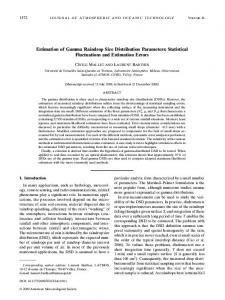
FIG. 1. (a) The spectral differential reflectivity for different raindrop size–shape relations. (b) Changes in the spectral differential reflectivity due to changes in the spectral broadening kernel width.

If radar measurements are taken at an elevation angle ranging between 30° and 60°, one can combine dual-polarization observations with Doppler spectra observations to get more insight into precipitation microphysics (Moisseev et al. 2006). In cases of no spectrum broadening and no wind, the spectral differential reflectivity can be defined as Zdr共␷兲 ⫽

hh Spr 共␷兲 vv Spr 共␷兲

⫽

␴hh共D兲 ␴vv共D兲

.

共5兲

One can see that in this particular case the spectral differential reflectivity depends only on two copolarized-scattering cross sections. This ratio is fully defined by raindrop shapes and therefore can be related to an existing raindrop size—shape relation, as can be seen in Fig. 1a. It is a continuing debate about a naturally occurring raindrop size–shape relation. As a result there is a number of known relations that are either based on experimental observations (Andsager et al. 1999; Prup-

pacher and Beard 1970; Chandrasekar et al. 1988; Bringi et al. 1998; Thurai et al. 2006), theoretical considerations (Beard and Chuang 1987), or a combination of both (Brandes et al. 2002). In Fig. 2 we have depicted some of the known relations and the corresponding spectral differential reflectivities are shown in Fig. 1a). From these two figures one can observe that differences in the shapes for diameters between 0.5 and 4 mm are the most important for the spectral differential observations. The relative unimportance of raindrop shapes for diameters larger than 4 mm is caused by nonlinearity of the expression (4). The effect of an assumed axis ration relation on the retrieval will be discussed later. In reality, Zdr(␷) observations are influenced by spectral broadening and the resulting observation can be expressed as

Zdr共␷兲 ⫽

冕冕

冉冉

hh Spr 共␷˜ 兲 exp ⫺

vv Spr 共␷˜ 兲

exp ⫺

冊冏冏冊冏冏

共␷ ⫺ ␷˜ ⫺ ␷0兲2

2␴ b2 共␷ ⫺ ␷˜ ⫺ ␷0兲2

2␴ b2

dD d␷˜ d␷ dD d␷˜ d␷

.

共6兲 The resulting Zdr(␷) values depend not only on parameters of the broadening kernel and raindrop shape–size relation but also on a DSD. Assuming an exponential relation (Bringi and Chandrasekar 2001) with Nw ⫽ 8000 mm⫺1 m⫺3 and D0 ⫽ 1.2 mm we have plotted Zdr (␷) in Fig. 1b for different values of the spectrum broadening kernel width. One can observe a strong dependence of Zdr(␷) on the spectrum broadening width. It should be noted that a nonzero wind radial velocity

JUNE 2007

1011

MOISSEEV AND CHANDRASEKAR TABLE 1. Simulation settings.

Frequency (GHz)

Pulse repetition rate (ms)

FFT length

␪ (°)

Nav

Nw

D0 (mm)

R (mm h⫺1)

␴b (m s⫺1)

␷0, (m s⫺1)

␳hv

Drop shape model

2.7

1

256

30

100

8000

1.2

4.6

0.5

0

0.99

Andsager et al. (1999)

would translate the spectral differential reflectivity, defined by (6), along the velocity axis.

3. DSD retrieval

(2), and ␷max is the value of the radial component of the largest raindrop terminal velocity (here it is assumed that raindrops with diameters of 0 to 8 mm are present in the radar volume). The coherency spectrum Whv(␷) is defined as follows:

a. Methodology To retrieve drop size distributions from Doppler spectra measurements, one needs to compensate for the effect of spectrum broadening and wind. Gossard (1988) and Rajopadhyaya et al. (1993) have shown that VHF profiler measurements of clear-air and precipitation returns can be used to estimate raindrop size distributions. The wind-profiling DSD retrieval procedure is based on deconvolution of an observed precipitation spectrum (1) by using a clear-air signal spectrum as the broadening kernel (Gossard 1988; Rajopadhyaya et al. 1993). This method gives a direct way of retrieving raindrop size distributions from VHF Doppler radar observations. For shorter wavelength radars, scattering from hydrometers is much larger than Bragg scattering, and therefore this method is not always applicable. Let us consider dual-polarization slant profile spectral measurements taken at an elevation angle ranging between 30° and 60°. In the previous section it was shown that in the absence of spectral broadening and wind the spectral differential reflectivity is completely defined by a drop size–shape relation. Assuming that this relation is known, one can use expression (5) as the reference differential reflectivity spectrum that corresponds to Doppler power spectra due to scattering from hydrometeors, as given by expression (3). The expression (5) is independent of a DSD. Therefore, the estimation procedure of the spectrum broadening kernel width and wind radial velocity component can be formulated as a least squares problem of finding parameters ␴b and ␷0 that minimize the sum square residuals, SSR: ␷max

SSR ⫽ M共␷兲 ⫽

冋

兺

dec M共␷兲 Zdr 共␷兲 ⫺

1,

Whv共␷兲 ⱖ 0.95

0,

otherwise.

␷⫽0

再


册

Whv共␷兲 ⫽

|Shv共␷兲|

公Shh共␷兲Svv共␷兲

,

共8兲

where Shv(␷) is the cross spectrum between hh and vv signals, and Shh(␷) and Svv(␷) are observed copolar power spectra. From expression (7) it can be seen that the coherency spectrum is used to eliminate parts of the spectral reflectivity that are affected by noise and clutter, as discussed in Moisseev et al. (2000).

b. Practical implementation and simulation results To illustrate feasibility of the procedure we have simulated dual-polarization radar observations using the method described by Chandrasekar et al. (1986). For these simulations the shape of spectra was assumed to be determined by expressions (1) and (3), where the

2

, 共7兲

Here Zdec dr (␷) is obtained by applying the deconvolution to the observed hh and vv power spectra with a convolution kernel Sb(␷ ⫺ ␷0, ␴b) defined by the expression

FIG. 3. The dependence of the cost function, (7), on the wind velocity and broadening kernel width. The white cross shows the solution of the optimization problem (9). The spectrum was simulated using the following input parameters: Nw ⫽ 8000 mm⫺1 m⫺3, D0 ⫽ 1.2 mm, ␮ ⫽ 0, ␷0 ⫽ 0 m s⫺1, and ␴b ⫽ 0.6 m s⫺1. The difference between input and retrieved values of ␴b can be explained by spectrum broadening due to use of the Chebyshev window.

1012


VOLUME 24

FIG. 4. An illustration of the method performance on the simulated data. The measurement elevation angle is 30°. (top) Power spectra before and after the deconvolution, represented by gray and solid line with x markers, respectively. Also for comparison purposes the model spectrum defined by the expression (3) is shown by the dashed line. (middle) The spectral differential reflectivity before and after the deconvolution. (bottom) The corresponding coherency spectra.

drop size distribution follows gamma functional form (Bringi and Chandrasekar 2001, section 7.1.4). The input parameters to this simulation are given in the Table 1. For each simulation run Doppler spectra were estimated by averaging over 30 simulated spectra. The DSD retrieval procedure consists of three steps. At the first step parameters of the convolution kernel are found. As described above this step is carried out by solving the following minimization problem: ␷max

min

兺

␷ 0,␴b ␷⫽0

冋

dec M共␷兲 Zdr 共␷兲 ⫺


册

2

.

共9兲

To deconvolve Doppler spectra we have used the iterative technique proposed by Lucy (1974). This deconvo-

lution technique is based on Bayes’ theorem on conditional probabilities and maximizes likelihood of an observed sample. An example of the cost function for one of the simulation runs is shown in Fig. 3. It was observed that in most of the cases the cost function (7) is well behaved. However, in some cases the function can have several local minima, as can be seen in Fig. 3, which can be associated with instabilities in the deconvolution process. To obtain a spectral broadening width and wind velocity component that correspond to a global minimum, the optimization procedure is initiated using several seed values. The seed values are selected randomly from a range of values in which the spectrum broadening width and wind velocity are expected to lie. One can observe that the solution of the problem (9)

JUNE 2007

1013


FIG. 5. An example of the retrieved and input drop size distribution. The retrieved DSD is depicted by the gray line with star markers, and the input DSD is shown by the solid line. The retrieval is based on the simulated spectrum shown in Fig. 4.

FIG. 6. The std dev and bias of the log N(D). The calculations are based on 100 simulations of Doppler spectra. The simulation specifications are given in Table 1.

gives the wind velocity component and spectrum broadening width values that are close to the input ones. For this simulation the spectrum broadening width was equal to 0.5 m s⫺1 and ambient wind velocity 0 m s⫺1. It should be noted that the difference between input and retrieved kernel width values can be attributed to the effect of spectrum window. The Chebyshev window with the sidelobe level of ⫺50 dB is used for spectral estimation. At the second step the convolution kernel is used to recover Spr(␷). In Fig. 4 simulated and recovered power spectra, spectral differential reflectivity, and coherency spectra are shown. It can be seen that the recovered spectrum, solid line with crosses, closely follows the modeled spectrum where ␴b ⫽ 0. It is interesting to note that the deconvolution procedure did not affect much the coherency spectrum values in the precipitation region. That comes from the fact that the values of the coherency spectrum in the precipitation region of the spectrum are not influenced by the spectrum broadening. Similar to the copolar correlation coefficient the copolar coherency spectrum is related to the statistical correlation between hh and vv radar signals.

In the final step the drop size distribution is estimated using the following expression: N共D兲 ⫽

Sˆ pr共␷兲 dD ␴共D兲 d␷

冏冏

共10兲

.

where the deconvolved power spectrum, Sˆ pr(␷), ideally should approach Spr(␷) defined by the expression (3). In the Fig. 5 the resulting DSD is shown. To assess the accuracy of this method 100 simulation runs were carried out. The resulting bias and standard deviation of the retrieved log N(D) is shown in Fig. 6. One can observe that under current assumptions bias in the log N(D) is less than 0.2 and the standard deviation in log N(D) is less than 1 for diameters less than 7 mm. Also, estimated D0, rain-rate values, and corresponding standard deviations are given in Table 2. The sensitivity of the proposed DSD retrieval method on the input DSD parameters was also tested. For this test input D0 values were varying from 0.5 to 2.5 mm with a step of 0.5 mm, and ␮ were varying from 0 to 5 with a step of 1. The remaining input parameters

TABLE 2. Results of the simulation. Estimated values of D0 and R and the std devs of the estimates. The input D0 value is 1.2 mm and the rain rate is 4.6 mm h⫺1. Est ⬅ estimated.

AB

D0 (mm) R (mm h⫺1)

AB retrieved with PB

Zdr bias 0.1 dB

Zdr bias 0.2 dB

Zdr bias 0.5 dB

Zdr bias 0.2 dB (corrected)

Std dev

Est

Std dev

Est

Std dev

Est

Std dev

Est

Std dev

Est

Std dev

Est

0.12 0.7

1.18 4.67

0.14 2.12

0.62 10.4

0.15 1.53

0.94 6.58

0.17 2.45

0.64 10.0

0.3 4.22

0.31 27.4

0.29 2.09

1.13 5.32

1014


VOLUME 24

Based on these simulations it was observed that a minimum drop diameter that can successfully be resolved is 0.3–0.4 mm and the maximum resolvable drop diameter is 7–8 mm. Due to increased errors in N(D) for small equivolumetric diameters, retrieved D0 values have larger errors in cases where input D0 values were smaller than 1 mm, as shown in Fig. 7. This effect is caused by the edge effects of the deconvolution procedure, where edges of deconvolved spectra have larger errors, and not by dependence of Zdr on D0. As a matter of fact, the reference spectral differential reflectivity is independent of DSD parameters. In Fig. 7 the bias and standard deviation of the retrieved D0 are shown. It was observed that the bias and the standard deviation do not exhibit dependence on ␮; as a result the presented results are averaged over all simulations with different input ␮ values. FIG. 7. Normalized (left) bias and (right) std dev of estimated D0 as functions of input D0.

are given in the Table 1. Comparing results of the simulation, given in the Table 2, with an error analysis of the dual-frequency technique shown in Schafer et al. (2002), one may conclude that these two techniques have comparable performances.

4. Evaluation of the methodology a. Effect of drop size–shape relation In the previous section we have shown that the proposed method is able to retrieve a DSD under the assumption that a raindrop size–shape relation is known. Currently there are a number of known relations that

FIG. 8. An effect of an assumed raindrop size–shape relation on the retrieval. (left) Retrieved and input DSD, depicted by solid and dashed lines respectively. The retrieved DSD is obtained by averaging the resulting DSD from 100 simulations. (right) A bias and standard deviation in the retrieved log N(D).

JUNE 2007


1015

FIG. 9. Influence of a Zdr offset on the retrieval. (left) A retrieved and input DSD. (middle) The biases in log N(D) for different Zdr offsets. (right) The std devs in the retrieved log N(D).

would result in different Zdr(␷) values especially for the diameters ranging between 0.5 and 4 mm, as shown in the Fig. 1. In this diameter range relations by Pruppacher and Beard (1970) and by Andsager et al. (1999) differ the most. Therefore, to study dependence of the proposed method on the raindrop shape assumption we have simulated 100 spectra using the Andsager et al. (1999) size–shape relation; the remaining input parameters are given in the Table 1. Then the spectrum broadening kernel width and wind velocity radial component were retrieved by solving (8), where the ratio [␴ hh(D)/␴vv(D)] was calculated assuming the (Pruppacher and Beard 1970) relation. The results of this study are given in the Fig. 8. It can be seen that as a result of the uncertainty in the drop size–shape relation, one might expect an increase in the log N(D) bias of the estimate for diameters less than 5 mm. In Table 2 retrieved values and standard deviation of D0 and rainrate estimates are shown. One can observe that an error

in the assumption has a strong result on the retrieved median volume diameter and rain rate.

b. Effect of Zdr calibration In the proposed method the retrieval of the spectrum broadening kernel width and wind velocity depends on Zdr(␷) observations and hence can be expected to be influenced by the calibration errors. To investigate this effect we have simulated three datasets of 100 spectra each, with Zdr offsets of 0.1, 0.2, and 0.5 dB, using parameters given in the Table 1. Then the DSD retrieval method was applied to each dataset. The results of this study are summarized in Fig. 9. It can be observed that Zdr offset has a strong influence on the bias in log N(D). It ranges between 0 and 0.5 for the offset of 0.1 dB, ⫺0.2 and 1 for the offset of 0.2 dB, and between ⫺1 and 1.7 for the offset of 0.5 dB. In the Table 2 the retrieved values of D0 and rain rate are shown. One can see that 0.1-dB Zdr offset results in

1016


VOLUME 24

TABLE 3. CSU–CHILL radar measurement settings.

Frequency

PRT

FFT length

Range resolution

␪ (°)

Polarization setting

No. of averages

2.7 GHz

1 ms

64

50 m

30

Alternating

270

about 20% standard error in the retrieved D0 and 40% in the retrieved rain rate. A 0.2-dB offset would result in 50% standard error in D0 and 120% error in the rain rate. And a 0.5-dB Zdr offset would result in underestimation of D0 by almost 4 times and overestimation of rain rate by almost 6 times. Another way of approaching this problem would be

to consider Zdr offset as an additional unknown parameter and to solve (8) for three parameters, ␴b, ␷0, and the offset. This approach was applied to the simulated radar observations with Zdr offset of 0.2 dB. The resulting DSD, bias, and standard deviation are shown in Fig. 9 as black solid lines. It can be seen that this approach reduces bias in the DSD estimate, which as a result

FIG. 10. Retrieved DSD from CSU–CHILL measurements. (left) Observed Doppler spectra at different ranges. (middle) Deconvolved spectra for given ranges. (right) Retrieved DSD, as depicted by solid lines. Moisseev et al. (2006) have shown that for this dataset logNw ⫽ 3.54, D0 ⫽ 1.2 mm, and ␮ ⫽ ⫺0.4, as shown by dashed lines.

JUNE 2007

1017


ranges between ⫺0.25 and 0.5, but it also increases the standard deviation of the estimate. And the retrieved values of D0 and rain rate have standard errors of 10% and 15%, respectively.

5. CSU–CHILL data On 23 July 2004 time series data measurements were collected during a stratiform rain event by the CSU– CHILL radar. The radar measurement settings are given in Table 3. The observed reflectivities for this event were around 35 dBZ. To investigate a performance of the DSD retrieval method, the observed spectra for each range gate were averaged over complete dataset. Prior to averaging, all spectra were shifted to the same mean velocity (Moisseev et al. 2006). Then the method was applied to the averaged spectra. For the estimation of the convolution kernel (Beard and Chuang 1987) raindrop shapes were assumed. The retrieved DSD were further averaged over five neighboring range gates, resulting in the effective range resolution of 250 m. The resulting raindrop size distributions for selected range gates are shown in Fig. 10. Moisseev et al. (2006) have used the same dataset to estimate precipitation DSD parameters by fitting the parametric model to the observed spectra. It was concluded that this measurement can be characterized by a gamma DSD with log Nw ⫽ 3.54, D0 ⫽ 1.2 mm, and ␮ ⫽ ⫺0.4. Moisseev et al. (2006) have also shown that the retrieved DSD parameters yield Zdr values comparable to the measured ones. The resulting log N(D) plot is shown in Fig. 10. One can observe that DSD retrievals from these two methods are in good agreement. The proposed nonparametric DSD retrieval method, nonetheless, shows more detail in the observed DSD.

6. Discussion and conclusions In this paper we have proposed a new nonparametric method for the retrieval of drop size distributions. This method does not use any assumption on the form of a DSD. It was shown that this method allows for an accurate DSD retrieval over large range of diameters. Since this is a radar-based retrieval method the accuracy of a retrieved DSD does not suffer from a small observation volume. This method is based on slant profile dual-polarization radar observations and does not require radar sensitivity to the Bragg scatter. As a result the proposed retrieval technique can be used by most dual-polarization radars. Acknowledgments. The research was supported by the National Science Foundation (ATM-0313881).

REFERENCES Andsager, K., K. V. Beard, and N. F. Laird, 1999: Laboratory measurements of axis ratios for large raindrops. J. Atmos. Sci., 56, 2673–2683. Atlas, D., R. S. Srivastava, and R. S. Sekhon, 1973: Doppler radar characteristics of precipitation at vertical incidence. Rev. Geophys. Space Sci., 11, 1–35. Beard, K. V., and C. Chuang, 1987: A new model for the equilibrium shape of raindrops. J. Atmos. Sci., 44, 1509–1524. Brandes, E. A., G. Zhang, and J. Vivekanandan, 2002: Experiments in rainfall estimation with a polarimetric radar in a subtropical environment. J. Appl. Meteor., 41, 674–685. Bringi, V. N., and V. Chandrasekar, 2001: Polarimetric Doppler Weather Radar: Principles and Applications. Cambridge University Press, 636 pp. ——, ——, and R. Xiao, 1998: Raindrop axis ratios and size distributions in Florida rainshafts: An assessment of multiparameter radar algorithms. IEEE Trans. Geosci. Remote Sens., 36, 703–715. ——, ——, J. Hubbert, E. Gorgucci, W. L. Randeu, and M. Schoenhuber, 2003: Raindrop size distribution in different climatic regimes from disdrometer and dual-polarized radar analysis. J. Atmos. Sci., 60, 354–365. Chandrasekar, V., V. Bringi, and P. Brockwell, 1986: Statistical properties of dual-polarized radar signals. Preprints, 23d Conf. on Radar Meteorology, Snowmass, CO, Amer. Meteor. Soc., 193–196. ——, W. A. Cooper, and V. N. Bringi, 1988: Axis ratios and oscillations of raindrops. J. Atmos. Sci., 45, 1323–1333. Currier, P. E., S. K. Avery, B. B. Balsley, and K. S. Gage, 1992: Use of two wind proflers for precipitation studies. Geophys. Res. Lett., 19, 1017–1020. Doviak, R. J., and D. S. Zrnic, 1993: Doppler Radar and Weather Observations. Academic Press, 562 pp. Gossard, E. E., 1988: Measuring drop-size distributions in clouds with a clear-air sensing Doppler radar. J. Atmos. Oceanic Technol., 5, 640–649. Jameson, A. R., and A. B. Kostinski, 2001: What is a raindrop size distribution? Bull. Amer. Meteor. Soc., 82, 1169–1176. Hauser, D., and P. Amayenc, 1981: A new method for deducing hydrometeor-size distributions and vertical air motions from Doppler radar measurements at vertical incidence. J. Appl. Meteor., 20, 547–555. Kezys, V., E. Torlaschi, and S. Haykin, 1993: Potential capabilities of coherent dual polarization X-band radar. Preprints, 26th Int. Conf. on Radar Meteorology, Norman, OK, Amer. Meteor. Soc., 106–108. Lucy, L. B., 1974: An iterative technique for the rectification of observed distributions. Astron. J., 79, 745–754. May, P. T., and T. D. Keenan, 2005: Evaluation of microphysical retrievals from polarimetric radar with wind profiler data. J. Appl. Meteor., 44, 827–838. ——, A. R. Jameson, T. D. Keenan, and P. E. Johnston, 2001: A comparison between polarimetric and wind profiler observations of precipitation in tropical showers. J. Appl. Meteor., 40, 1702–1717. ——, ——, ——, ——, and C. Lucas, 2002: Combined wind profiler/polarimetric radar studies of the vertical motion and microphysical characteristics of tropical sea-breeze thunderstorms. Mon. Wea. Rev., 130, 2228–2239. Moisseev, D. N., C. Unal, H. Russchenberg, and L. Ligthart, 2000: Polarimetric ground clutter identification and suppression for

1018


atmospheric on co-polar correlation. Proc. 14th Int. Conf. on Microwaves, Radar and Wireless Communications, Wroclaw, Poland, 94–97. ——, V. Chandrasekar, C. M. H. Unal, and H. W. J. Russchenberg, 2006: Dual-polarization spectral analysis for retrieval of effective raindrop shapes. J. Atmos. Oceanic Technol., 23, 1682–1695. Pruppacher, H. R., and K. V. Beard, 1970: A wind tunnel investigation of the internal circulation and shape of water drops falling at terminal velocity in air. Quart. J. Roy. Meteor. Soc., 96, 247–256. Rajopadhyaya, D. K., P. T. May, and R. A. Vincent, 1993: A general approach to the retrieval of rain drop-size distributions from VHF wind profiler Doppler spectra: Modeling results. J. Atmos. Oceanic Technol., 10, 710–717. Russchenberg, H. W. J., 1993: Doppler polarimetric radar measurements of the gamma drop size distribution of rain. J. Appl. Meteor., 32, 1815–1825. Schafer, R., S. Avery, P. May, D. Rajopadhyaya, and C. Williams, 2002: Estimation of rainfall drop size distributions from dualfrequency wind profiler spectra using deconvolution and a nonlinear least squares technique. J. Atmos. Oceanic Technol., 19, 864–874. Seliga, T. A., and V. N. Bringi, 1976: Potential use of the radar reflectivity at orthogonal polarizations for measuring precipitation. J. Appl. Meteor., 15, 69–76. ——, and ——, 1978: Differential reflectivity and differential phase shift: Applications in radar meteorology. Radio Sci., 13, 271–275. Spek, A. L. J., D. N. Moisseev, H. W. J. Russchenberg, C. M. H. Unal, and V. Chandrasekar, 2005: Retrieval of microphysical properties of snow using spectral dual-polarization analysis. Preprints, 32d Conf. on Radar Meteorology, Albuquerque, NM, Amer. Meteor. Soc., CD-ROM, P11R.10. Thurai, M., G. J. Huang, V. N. Bringi, and M. Schonhuber, 2006:

VOLUME 24

Drop shape probability contours in rain from 2-D video disdrometer: Implications for the “self consistency method” at C-band. Proc. Fourth European Conf. on Radar in Meteorology and Hydrology, Barcelona, Spain, 25–29. Ulbrich, C. W., 1983: Natural variations in the analytical form of raindrop size distributions. J. Climate Appl. Meteor., 22, 1764–1775. ——, and D. Atlas, 1998: Rain microphysics and radar properties: Analysis methods for drop size spectra. J. Appl. Meteor., 37, 912–923. Unal, C. M. H., D. N. Moisseev, and L. P. Ligthart, 1998: Dopplerpolarimetric radar measurements of precipitation. Proc. 4th Int. Workshop on Radar Polarimetry (JIRP ’98), Nantes, France, IRESTE, 429–438. ——, ——, H. Russchenberg, and L. Ligthart, 2001: Radar Doppler polarimetry applied to precipitation measurements: Introduction of the spectral differential reflectivity. Preprints, 30th Conf. on Radar Meteorology, Munich, Germany, Amer. Meteor. Soc., 316–318. Wakasugi, K., A. Mizutani, M. Matsuo, S. Fukao, and S. Kato, 1986: A direct method for deriving drop size distribution and vertical air velocities from VHF Doppler radar spectra. J. Atmos. Oceanic Technol., 3, 623–629. Williams, C. R., 2002: Simultaneous ambient air motion and raindrop size distributions retrieved from UHF vertical incident profiler observations. Radio Sci., 37, 1024, doi:10.1029/ 2000RS002603. Willis, P. T., 1984: Functional fits to some observed drop size distribution and parameterization of rain. J. Atmos. Sci., 41, 1648–1661. Wilson, D. R., A. J. Illingworth, and T. M. Blackman, 1997: Differential Doppler velocity: A radar parameter for characterizing hydrometeor size distributions. J. Appl. Meteor., 36, 649–663.