Sep 20, 2016 - This article is published online with Open Access by IOS Press and .... Left: an update for the Pareto distribution with only 2 data points does not ...
STAIRS 2016 D. Pearce and H.S. Pinto (Eds.) © 2016 The authors and IOS Press. This article is published online with Open Access by IOS Press and distributed under the terms of the Creative Commons Attribution Non-Commercial License 4.0 (CC BY-NC 4.0). doi:10.3233/978-1-61499-682-8-203
203
Nonparametric Segment Detection Anne C. VAN ROSSUM a,c , Hai Xiang LIN b,c Johan DUBBELDAM b H. Jaap VAN DEN HERIK c a Crownstone B.V., Rotterdam, the Netherlands b Delft University of Technology, Delft, the Netherlands c Leiden University, Leiden, the Netherlands Abstract. In computer and robotic vision point clouds from depth sensors have to be processed to form higher-level concepts such as lines, planes, and objects. Bayesian methods formulate precisely prior knowledge with respect to the noise and likelihood of points given a line, plane, or object. Nonparametric methods also formulate a prior with respect to the number of those lines, planes, or objects. Recently, a nonparametric Bayesian method has been proposed to perform optimal inference simultaneously over line fitting and the number of lines. In this paper we propose a nonparametric Bayesian method for segment fitting. Segments are lines of finite length. This requires 1.) a prior for line segment lengths: the symmetric Pareto distribution, 2.) a sampling method that handles nonconjugacy: an auxiliary variable MCMC method. Results are measured according to clustering performance indicators, such as the Rand Index, the Adjusted Rand Index, and the Hubert metric. Surprisingly, the performance of segment recognition is worse than that of line recognition. The paper therefore concludes with recommendations towards improving Bayesian segment recognition in future work. Keywords. Nonparametric Bayesian, segment detection
Introduction In computer vision there are many practical methods to extract lines out of a collection of point observations. Straight line extraction can be done by the Hough transform [3], RANSAC [2], and is known in general as linear regression. Linear regression can be cast as a Bayesian inference model by defining a likelihood for observations given line parameters and a prior for the line parameters themselves. If the prior for the line parameters is a normal distribution, this corresponds to ridge regression (l2 norm). If the prior for the line parameters is a Laplace distribution, this corresponds with lasso (l1 norm). Bayesian linear regression for a single line is well understood. A challenge arises when multiple lines have to be extracted simultaneously. Observations have to be partitioned over lines as well as fitted to the line to which they belong. For multiple lines, a Bayesian method postulates a prior with respect to the line parameters as well as the distribution of points over the lines. Given a multinomial distribution of points over lines, a Dirichlet Process mixture has been used as such a prior before [5].
204
A.C. van Rossum et al. / Nonparametric Segment Detection
A Bayesian model of linear regression does not take into account the length of the lines. If it is known that lines are of finite length, this information can be used to enrich the prior. In the real world, if the height of a person is known to a robot it can use this as a prior in a recognition task. To detect the number of line segments, we require a model for the line segment, priors for the line arguments, and a model and prior for the distribution of points over the line segments. In this paper we show that including the fact that the lines are of finite length will not lead to an improvement in segment detection compared to unconstrained inference. 1. Mixture model for line segments The model consists out of two parts. The segment model (Sect. 1.1) defines how an individual segment is described as the sampling of pairs of points from a shifted symmetric Pareto distribution. The Dirichlet Process Mixture (Sect. 1.2) is a mixture of multiple of such segments using a Dirichlet Process as prior. 1.1. Segment model There seems to be no statistical description of data points distributed over a line segment that has a conjugate prior form. A line segment itself, however, has a conjugate form! Suppose that we have a prior for the location of endpoints on the x-axis. By postulating a uniform distribution of the data across the segment, we can find the new location of the endpoints using a conjugate Bayesian construction. Uniform likelihood The data x is distributed according to a symmetric uniform distribution between −a and a. Hence the likelihood is given by Eq. 1. � x | a ∼ U (x; a) =
1 2a
0
for x ≤ |a| otherwise
(1)
Pareto prior A prior for the (endpoints of a) symmetric uniform distribution is a symmetric Pareto distribution, Ps . � a ∼ Ps (a; λ, k) =
1 k −k−1 2 kλ |a|
0
|a| ≥ λ otherwise
(2)
Pareto pairs To sample endpoints of segments we have to sample 1.) pairs of points (just as many left as right endpoints), and 2.) shift the distribution. p(a, b) ∼ Pp (a, b; λm , λn , k)
(3)
The right endpoint is sampled from a normal Pareto distribution with λm and the left endpoint from a mirrored Pareto distribution with λn . The sampling of Pareto pairs is visualized in Fig. 1.
A.C. van Rossum et al. / Nonparametric Segment Detection
205
Figure 1. Sampling of N = 1000 Pareto pairs. The parameters are λm = 2, λn = −4, k = 5, hence the distribution is centered around −1. There are 500 data points sampled for the left endpoint, 500 data points for the right endpoint.
Conjugate The Pareto distribution is a conjugate prior for a likelihood described by a uniform distribution. The hyperparameters for the posterior Pareto distribution are updated as in Eq. 4. p(a | x0 , . . . , xN −1 ) = P(c, N + k)
(4)
The parameter k is adjusted with the number of data points N , and the parameter c is the maximum of {m, λ} with m the maximum value in x0 , . . . , xN −1 .
Figure 2. Data uniformly distributed on line segment [−4, 5] with a Pareto pair prior for the endpoints. Left: an update for the Pareto distribution with only 2 data points does not set the left endpoint to −4 yet. Right: further updates of the Pareto distribution with 100 data points sets endpoints to −4 and 5.
Sampling from the Pareto distribution is through inverse transform sampling. By sampling from U (0, 1) with 1 included, we transform according to k/U 1/a . Fig. 2 shows how the endpoints are updated given the data. An uninformative prior is used. In this case the hyperparameters λn,0 and λm,0 are set close to 0, thus the data will wash out the prior immediately. Note that update of a Pareto distribution using a maximum operator: if λm is set to a large value, it will never get smaller with more observations. 1.2. Dirichlet Process Mixture The distribution of points over line segments is defined as a Dirichlet Process prior.
A.C. van Rossum et al. / Nonparametric Segment Detection
206
α
zi
π
wi N
θk
H
∞
Figure 3. The Bayesian linear regression model for multiple line segments in plate notation. From left to right: The Dirichlet Process’s concentration parameter α that defines the density of observations within clusters. The partitions (π1 , . . . , πk ) with assignment parameters zi that denote which observation wi belongs to which cluster k. The cluster is summarized through parameter θk (slope, y-intercept, segment size), generated from the base distribution H(λ0 ).
In Fig. 3 the model is visualized in plate notation and concisely described in Eq. 5. G ∼ DP (α, H) θi | G ∼ G
(5)
wi | θi ∼ F (wi |θi ) F describes the mapping from parameters θi to observations wi = (Xi , yi ). The probability density F is the product of a Gaussian distribution over the line y − Xβ (with σ 2 as variance) and an uniform distributed between [a, b] on the x-axis. F (wi |θi ) = F (yi |Xi , β, σ 2 , a, b) = N (yi − Xi β, σ 2 )U (Xi ; a, b)
(6)
2. Inference over a line segment Regardless of the existence of a conjugate prior of the above likelihood description, there are sampling algorithms that do not demand conjugacy. One of these algorithms uses auxiliary variables [1,4] that postulate not just one single new cluster to assign observations to, but multiple new clusters with different parameters each. To establish to which cluster a certain observation wi needs to be assigned, the likelihood of each existing and new cluster is compared. The weight of an old cluster is defined through the number of data points assigned to it. The weight of a new cluster is defined through α/m. See for further details Algorithm 1. 3. Results There is one phenomenon that is very noticable in Fig. 4. Line segments that form a larger line segment are not recognized as such by the inference method. The results over a larger dataset can be measured with clustering metrics as visualized in Fig. 5. The Rand Index, Adjusted Rand Index, and Hubert metrics show all reduced performance compared to line detection where there are no constraints on segment size.
A.C. van Rossum et al. / Nonparametric Segment Detection
(a) Correctly sampled. Only one outlier to the left.
(b) Incorrectly sampled. The line is recognized as multiple segments.
(c) More or less correct. The segments with fewer observations are recognized poorly.
(d) Completely incorrect. Line segments are chosen to be orthogonal to the lines.
207
Figure 4. Bayesian point estimates of the sampling process with varying outcomes.
(a) Segment detection.
(b) Line detection.
Figure 5. Segment detection performs much worse than line detection across all three clustering performance indicators. Perfect clustering is indicated by 1.0 for Rand Index, Adjusted Rand Index, and Hubert.
4. Conclusion Inference over a mixture of lines might benefit from information about line length. We constrained lines to segments by postulating a prior over segment sizes. How-
A.C. van Rossum et al. / Nonparametric Segment Detection
208
ever, no improved performance was yielded by this approach. The Dirichlet Process prior (the concentration parameter α) is not strong enough to prevent subdivision of a segment into subsegments (connected head to tail). To overcome this in future work, we can 1.) use an improved Gibbs sampler with sample steps that merge smaller segments into larger segments, or 2.) use a likelihood function in which the distribution of points over a segment is taken into account.
References [1]
P Damlen, John Wakefield, and Stephen Walker. Gibbs sampling for Bayesian nonconjugate and hierarchical models by using auxiliary variables. Journal of the Royal Statistical Society: Series B (Statistical Methodology), 61(2):331–344, 1999. [2] Martin A. Fischler and Robert C. Bolles. Random Sample Consensus: A Paradigm for Model Fitting with Applications to Image Analysis and Automated Cartography. Commun. ACM, 24(6):381–395, June 1981. [3] Paul V.C. Hough. Method and Means for Recognizing Complex Patterns, Dec 1962. Patent US 3069654 A. [4] Radford M Neal. Markov chain sampling methods for Dirichlet process mixture models. Journal of computational and graphical statistics, 9(2):249–265, 2000. [5] Anne C. van Rossum, Hai Xiang Lin, Johan Dubbeldam, and H. Jaap van den Herik. Nonparametric Bayesian Line Detection - Towards Proper Priors for Robotic Computer Vision. In Proceedings of the 5th International Conference on Pattern Recognition Applications and Methods, pages 119–127, Feb 2016.
Algorithm 1 Gibbs sampling over auxiliary variables 1: procedure Gibbs Algorithm with auxiliary variables(w, λ0 , α)
2: 3: 4: 5: 6: 7: 8: 9: 10: 11: 12: 13: 14: 15: 16: 17: 18: 19: 20:
� Accepts points w, hyperparameters λ0 , α, number of auxiliary variables m, and returns k line segment parameters for all t = 1 : T do for all i = 1 : N do for all j = 1 : m do θj ∼ N IG(λ0 ) � Sample θj from NIG end for for all j = 1 : K + m, j �= i do Lj = F (wi |θj ) � Update likelihood for all theta (except θi ) end for � P−i=1:K = b −i L−i � Calculate probability of existing cluster P−i=K:K+m = bα/mLm L−i � Calculate probability of new cluster θi = θj according to above P−i � Sample θi accord. to above prob Remove unused clusters end for for all j = 1 : K do θj ∼ p(θj | y) � Update θj end for end for return summary on θk for k line segments end procedure