International Journal of Statistics and Probability; Vol. 6, No. 5; September 2017 ISSN 1927-7032 E-ISSN 1927-7040 Published by Canadian Center of Science and Education
Nonparametric Tests for Convexity/Monotonicity/Positivity of Multivariate Functions with Noisy Observations Eunji Lim1 & Elizabeth Tavarez2 1
College of Business and Public Administration, Kean University, Union, NJ 07083, USA
2
College of Business and Public Administration, Kean University, Union, NJ 07083, USA
Correspondence: Eunji Lim, College of Business and Public Administration, Kean University, Union, NJ 07083, USA. E-mail:
[email protected] Received: June 7, 2017
Accepted: July 3, 2017
doi:10.5539/ijsp.v6n5p18
Online Published: July 21, 2017
URL: https://doi.org/10.5539/ijsp.v6n5p18
Abstract We propose a new method of testing for a function’s convexity, monotonicity, or positivity, based on some noisy observations of the function made over a finite set T of points in the domain, where the observations can be made multiple times at each point in T . One of the traditional approaches to the test of a function’s shape characteristic is to fit a convex, a monotone, or a positive function, depending on the shape characteristic we wish to test for, to the data set minimizing the sum of squared errors, and to compute the sum of squared differences (SSD) between the fit and the data set. While the traditional approach proceeds by observing the SSD as the number of points in T increases to infinity, we propose observing the SSD as r, the number of observations taken at each point in T , increases to infinity. This new way of observing the asymptotic behavior of the SSD leads to a test procedure that does not require the estimation of any additional parameters, and hence, is easy to implement. The proposed test procedure is proven to achieve a prescribed power as r → ∞. Numerical examples illustrate that the proposed test successfully detects the convexity/monotonicity/positivity of a function, as well as the non-convexity/non-monotonicity/non-positivity of a function. Keywords: convexity detection, monotonicity detection, positivity detection, hypothesis test, convex regression, isotonic regression, nonparametric test, multivariate regression 1. Introduction The goal of this paper is to develop a hypothesis test for determining whether an unknown function f∗ : Rd → R is convex, monotone, or positive using some noisy measurements of f∗ at points X1 , . . . , Xn ∈ Rd . The convexity/monotonicity/positivity of a function has significant implications in many areas of applications. In economics, the concavity of the utility curve as a function of a person’s income implies that the marginal utility diminishes as income increases (p. 31 of Keynes, 1935). In the context of statistical inference, the monotonicity of a function that one wishes to estimate from noisy data indicates that one can fit a monotone function to the data set to reconstruct the underlying function (Barlow et al., 1972). In this paper, we assume that we can observe noisy measurements of f∗ (Xi ) for 1 ≤ i ≤ n, and these observations can be made multiple times independently of each other. Thus, we are able to obtain the data set ((Xi , Yi j ) : 1 ≤ i ≤ n, 1 ≤ j ≤ r), where Yi j = f∗ (Xi ) + ϵi j , the Xi ’s are either Rd -valued random vectors or deterministic points in Rd , and the ϵi j ’s are independent and identically distributed (iid) random variables with E(ϵi j | X1 , . . . , Xn ) = 0 and E(ϵi2j | X1 , . . . , Xn ) = σ2 for some σ < ∞. To determine whether the function f∗ is convex/monotone/positive or not, we consider the following pairs of the null and alternative hypotheses: Null Hypothesis Hc0 Hm0 H 0p
Alternative Hypothesis
: f∗ < F c
Hca : f∗ ∈ Fc
: f∗ < F m
Hma H ap
: f∗ < F p
for a test of convexity,
: f∗ ∈ Fm
for a test of monotonicity,
: f∗ ∈ F p
for a test of positivity,
18
http://ijsp.ccsenet.org
International Journal of Statistics and Probability
-1.00
-0.60
-0.20
0.20
0.60
Vol. 6, No. 5; 2017
1.00
Figure 1. The solid line is f∗ and the dashed line is the function to which fˆc converges as r → ∞.
where Fc Fm Fp
= = =
{g : Rd → R | g(tv + (1 − t)w) ≤ tg(v) + (1 − t)g(w) for v, w ∈ Rd and t ∈ [0, 1]}, {g : Rd → R | g(v) ≤ g(w) for v = (v(1), . . . , v(d)) and w = (w(1), . . . , w(d)) ∈ Rd with v(k) ≤ w(k), 1 ≤ j ≤ d} {g : Rd → R | g(v) ≥ 0 for v ∈ Rd }.
When the context is clear, Hc0 , Hm0 , and H 0p will be referred to as the null hypotheses and Hca , Hma , and H ap the alternative hypotheses. The proposed test procedure is described as follows. Test of Convexity: When one suspects that the unknown function f∗ is convex, a natural step to take in order to estimate ∑ f∗ is to fit a convex function fˆc : Rd → R to the data set ((Xi , Y i ) : 1 ≤ i ≤ n), where Y i = rj=1 Yi j /r for 1 ≤ i ≤ n, which minimizes the sum of squared distances between the fit and the data set. The fitted function fˆc can be defined by the solution to the following infinite-dimensional minimization problem: )2 1 ∑( Y i − g(Xi ) n i=1 n
Minimize
(1)
over g ∈ Fc . Problem (1) turns out to be equivalent to the following finite-dimensional quadratic programming problem: Minimize
n )2 1 ∑( Y i − g(Xi ) n i=1
Subject to
g(X j ) ≥ g(Xi ) + ξiT (X j − Xi ),
(2) 1 ≤ i, j ≤ n
in the decision variables g(Xi ) ∈ R and ξi ∈ Rd for 1 ≤ i ≤ n, where ξiT denotes the transpose of ξi (Lemma 2.5 of Seijo & Sen, 2011). When f∗ is truly convex, the mean square error (MSE), defined by n )2 1 ∑( Y i − fˆc (Xi ) , n i=1
∑ ∑ ∑ converges to 0 as r → ∞ because ni=1 (Y i − fˆc (Xi ))2 /n ≤ ni=1 (Y i − f∗ (Xi ))2 /n = ni=1 ϵ¯i /n → ∞ as n → ∞ by the ∑ minimizing property of fˆc and the strong law of large numbers, where ϵ¯i = rj=1 ϵi j /r for 1 ≤ i ≤ n. Proposition 1 of this paper also shows that the rate of convergence is of order 1/r. However, when f∗ is not convex, the MSE will possibly converge to a certain positive number as r → ∞ because fˆc converges to a function that is different from f∗ . Figure 2 shows a graph of f∗ , which is not convex, and the function to which fˆc converges as r → ∞. The test statistic of our proposed procedure is therefore the MSE multiplied by r as follows: )2 r ∑( Y i − fˆc (Xi ) n i=1 n
TSc
=
19
(3)
http://ijsp.ccsenet.org
International Journal of Statistics and Probability
Vol. 6, No. 5; 2017
The asymptotic behavior of the MSE suggests that we do not reject Hc0 if the test statistic TSc diverges to infinity as r → ∞. The critical value will be derived from Propositions 1 and 2 in Section 2 at a prescribed value of the Type II error. Test of Monotonicity: For a test of monotonicity, we will use a similar procedure. When one suspects that f∗ is monotone, one can fit a monotone function fˆm : Rd → R to the data set, which minimizes the sum of squared errors. The fitted function fˆm is the solution to the following quadratic program: Minimize
)2 1 ∑( Y i − g(Xi ) n i=1
Subject to
g(Xi ) ≤ g(X j ) for Xi = (Xi (1), . . . , Xi (d)) and X j = (X j (1), . . . , X j (d))
n
(4)
satisfying Xi (k) ≤ X j (k) for k = 1, . . . , d in the decision variables g(X1 ), . . . , g(Xn ) ∈ R. The proposed test statistic is then defined by )2 r ∑( Y i − fˆm (Xi ) n i=1 n
TSm
=
(5)
and Hm0 is not rejected if the test statistic TSm diverges to infinity as r → ∞. Test of Positivity: For the test of positivity, the proposed test statistic is given by )2 r ∑( Y i − fˆp (Xi ) , n i=1 n
TS p
=
(6)
where fˆp is the solution to the following quadratic program: Minimize
)2 1 ∑( Y i − g(Xi ) n i=1
Subject to
g(Xi ) ≥ 0, 1 ≤ i ≤ n
n
(7)
in the decision variables g(Xi ) for 1 ≤ i ≤ n. H 0p is not rejected if the test statistic TS p diverges to infinity as r → ∞. Tests of convexity/monotonicity/positivity have been widely studied in the statistics literature. Various types of hypothesis tests are proposed with different test statistics. However, most work in the literature has focused on observing the behavior of the test statistic as n → ∞ with a fixed value of r (Yatchew, 1992; Hall & Jeckman, 2000; Baraud et al., 2005) or imposed a condition that requires the normality of the ϵi j ’s (Bartholomew, 1959; Shapiro, 1988; Baraud et al., 2005). For example, the MSE has been studied as a test statistics in Shapiro (1988), but the behavior of the test statistic is studied only for the case where n → ∞ with r fixed. Empirical studies suggest that the weights used in Shapiro (1988) are difficult to compute exactly, so the test procedure proposed by Shapiro (1988) is computationally burdensome (Sen & Silvapulle, 2002). Bartholomew (1959) used the MSE as a test statistic, but he assumed that the ϵi j ’s are normally distributed and did not consider the case where r → ∞. Yetchew (1992) also considered the MSE as a test statistic, but did not consider the case where r → ∞, and focused only on the case where f∗ is defined on the one-dimensional set R. Others have used various types of test statistics to test a function’s convexity/monotonicity/positivity. For example, Ghosal et al. (2000) use a locally weighted version of Kendall’s tau statistic as a test statistic, whereas Wang & Meyer (2011) use regression splines and their derivatives to define a test statistic. In this paper, we take a different point of view from the existing literature. Even though increasing n to infinity may result in a good estimator of the true function f∗ (x) over all x ∈ Rd , increasing r to infinity can provide simpler and more practical tests for convexity/monotonicity/positivity detection that are easier to implement. We thus observe the asymptotic behavior of our test statistic as r → ∞ and derive the critical value accordingly. The critical value turns out to be a percentile of (σ2 /n)χ2n , where χ2n follows the chi-square distribution with n degrees of freedom. Considering the fact that σ2 can be easily estimated from the sample variance of Y11 , . . . , Y1r , the critical value can be readily computed from the data set. The situation where r is large arises frequently in practice. In particular, this situation arises when f∗ is an unknown function that we want to estimate using “computer simulation” and when we are able to select any point x in the domain of f∗ , get an estimate of f∗ (x) through computer simulation, and repeat this procedure as many times as we wish. For example, when f∗ is the price of a stock option that is contingent on the price x ∈ R of the underlying stock, we can use computer simulation to get an estimate of f∗ (x) at any point x as many times as we wish, and hence, r can be made as large as we wish. 20
http://ijsp.ccsenet.org
International Journal of Statistics and Probability
Vol. 6, No. 5; 2017
Our main contribution is therefore proposing a simple and practical test procedure that is based on the idea that the MSE converges to 0 as r → ∞ if f∗ is convex, and diverges to infinity as r → ∞ if f∗ is not convex. The proposed procedure does not require estimation of any additional parameters. Furthermore, it does not rely on any assumptions regarding the distribution of the Xi ’s and the ϵi j ’s. The test statistic and the critical value can be easily computed from the data set. This paper is organized as follows. In Section 2, we prove that the proposed test achieves a prescribed power as r → ∞. We also describe the proposed test procedure in more detail. In Section 3, we apply the proposed test to different types of f∗ , and observe the conclusion of our test as r → ∞. The numerical results in Section 3 illustrate that the proposed test successfully rejects the null hypothesis when the alternative hypothesis is true for r sufficiently large. Concluding remarks are included in Section 4. 2. The Asymptotic Behavior of the Test Statistics and the Proposed Test Procedure In order to analyze the behavior of the test statistics, we will impose some probabilistic assumptions on the ϵi j ’s. In particular, we require the following assumptions: A1. Given X1 , X2 , . . . , the ϵi j ’s are iid random values. ( ) A2. E ϵi j | X1 , . . . , Xn = 0 for 1 ≤ i ≤ n and 1 ≤ j ≤ r. ( ) A3. E ϵi2j | X1 , . . . , Xn = σ2 for 1 ≤ i ≤ n and 1 ≤ j ≤ r and for some σ < ∞ We first establish in Proposition 1 the fact that the asymptotic distribution of the test statistics defined in (3), (5), and (6) as r → ∞ is similar to the distribution of (σ2 /n)χ2n . Proposition 1 Assume A1–A3. Then, for a fixed n, n ( ) )2 r ∑ ( ˆ lim sup P Y i − fc (Xi ) > τ f∗ ∈ Fc ≤ P (σ2 /n)χ2n > τ , n i=1 r→∞ n ) ( )2 r ∑ ( ˆ lim sup P Y i − fm (Xi ) > τ f∗ ∈ Fm ≤ P (σ2 /n)χ2n > τ , n i=1 r→∞ n ( ) )2 r ∑ ( ˆ lim sup P Y i − f p (Xi ) > τ f∗ ∈ F p ≤ P (σ2 /n)χ2n > τ n i=1 r→∞ for any τ ≥ 0, where χ2n follows the chi-squared distribution with n degrees of freedom. Proof. We begin by proving the existence and the uniqueness of fˆc , fˆm , and fˆp . The existence and the uniqueness of fˆc is proven in Lemma 2.3 of Seijo & Sen (2011). To prove the existence of fˆm , we note that Problem (4) is a minimization problem of a coercive function over a non-empty closed subset of Rn . By Theorem 2.32 on page 25 of Beck (2014), the solution to Problem (4) exists. To prove the uniqueness of the solution, suppose on the contrary that Problem (4) has two distinct minimizers, say v = (v(1), . . . , v(n)) and w = (w(1), . . . , w(n)). Since φ : Rn → R, defined by φ(z) = ∑n 2 n i=1 (Y i − z(i)) /n for z = (z(1), . . . , z(n)) ∈ R , is strictly convex and (1/2)v + (1/2)w is a feasible solution to Problem (4), we must have φ((1/2)v + (1/2)w) < (1/2)φ(v) + (1/2)φ(w). Since φ(v) = φ(w), we have φ((1/2)v + (1/2)w) < φ(v), which contradicts the fact that v is a minimizer of Problem (4). Therefore, Problem (4) has a unique minimizer. The existence and the uniqueness of fˆp follows using similar arguments. Now, we are ready to prove the main statement of Proposition 1. Suppose f∗ ∈ Fc . Then, n n ( )2 1 ∑ )2 1 ∑( ˆ fc (Xi ) − Y i ≤ f∗ (Xi ) − Y i n i=1 n i=1 ) ∑ ( since f∗ is convex and fˆc minimizes ni=1 Y i − g(Xi ) /n over all convex functions g. Next, we will prove that
)2 r ∑ r ∑( σ2 2 χ f∗ (Xi ) − Y i = ϵ¯i2 ⇒ n i=1 n i=1 n n n
(8)
n
as r → ∞. To prove (9), we first note that, for any η ∈ R, n n r ∑ 2 r ∑ 2 P ϵ¯i > η = E P ϵ¯i > η X1 , . . . , Xn n i=1 n i=1 21
(9)
http://ijsp.ccsenet.org
International Journal of Statistics and Probability
Vol. 6, No. 5; 2017
n ( ) r ∑ 2 P ϵ¯i > η X1 , . . . , Xn → P (σ2 /n)χ2n > η n i=1
and that
almost surely as r → ∞ by the weak law of large numbers (A1, A2, and A3) and the continuous mapping theorem. ∑ Applying the bounded convergence theorem to P((r/n) ni=1 ϵ¯i2 > η | X1 , . . . , Xn ) yields n ( ) r ∑ 2 ϵ¯i > η X1 , . . . , Xn → P (σ2 /n)χ2n > η , E P n i=1 and hence, (9) follows. Combining (8) and (9) yields n n ( )2 )2 ( ) r ∑ ( r ∑ Y i − fˆc (Xi ) > τ ≤ P Y i − f∗ (Xi ) > τ → P (σ2 /n)χ2n ≥ τ P n i=1 n i=1 as r → ∞, and hence, the first inequality of Proposition 1 follows. The rest of Proposition 1 uses similar arguments.
2
Proposition 1 enables us to suggest the following test procedure. Proposed Hypothesis Test 1. Using the data set ((Xi , Y i ) : 1 ≤ i ≤ r), compute the test statistic TSc from (3) for a test of convexity, TSm from (5) for a test of monotonicity, and TS p from (5) for a test of positivity. 2. Let β be the prescribed value of the Type II error. In other words, β is the desired probability of not rejecting the null hypothesis when the alternative hypothesis is true. Let z1−β be the 100(1 − β)th percentile of (σ2 /n)χ2n . When σ2 ∑ is not known, σ2 can be estimated from the sample variance of Y11 , . . . , Y1r , i.e., rj=1 (Y1 j − Y 1 )2 /(r − 1). 3. If the test statistic is less than or equal to z1−β , then reject the null hypothesis in favor of the alternative hypothesis. Otherwise, do not reject the null hypothesis. The following proposition shows that the proposed test achieves the prescribed power as r → ∞. Proposition 2 Assume A1–A2. Then ( ) lim inf P Reject Hc0 | f∗ ∈ Fc ≥ 1 − β, r→∞ ( ) lim inf P Reject Hm0 | f∗ ∈ Fm ≥ 1 − β, r→∞ ( ) lim inf P Reject H 0p | f∗ ∈ F p ≥ 1 − β. r→∞
Proof. Since (
P Reject
Hc0
n ) ∑( )2 f ∈ F = P r Y i − fˆc (Xi ) ≤ z1−β c ∗ n i=1
n ∑( )2 f ∈ F = 1 − P r Y i − fˆc (Xi ) > z1−β c ∗ n i=1
f ∈ F , c ∗
it follows, by Proposition 1, that (
lim inf P Reject r→∞
Hc0
n ) ∑( )2 f ∈ F = 1 − lim sup P r Y i − fˆc (Xi ) > z1−β c ∗ n i=1 r→∞
f ∈ F > 1 − P ((σ/r)χ2 > z ) = 1 − β. 1−β c r ∗ 2
The rest of Proposition 2 uses similar arguments. 3. Numerical Results
In this section, we apply the proposed test procedure to various types of f∗ . We conduct the proposed hypothesis test for each case of f∗ , and observe whether the null hypothesis is rejected or not as we increase r. By repeating the procedure multiple times for each case of f∗ , we estimate the proportion of time that the null hypothesis is rejected. Numerical results in Sections 3.1, 3.2, and 3.3 display that the proportion of time that Hc0 , Hm0 , or H 0p is rejected converges to 1 as r increases 22
http://ijsp.ccsenet.org
International Journal of Statistics and Probability ݂1
1.5
݂2
1.5 1
1
0.5
0.5
0.5
0
1
21
41
61
݂4
1.5
0
1
21
41
61
݂5
1.5
1
1
1
0.5
0.5
0.5
0 1
21
41
61
81
݂7
1.5
21
41
61
81
݂8
1
0.5
0.5
0.5
0
21
21
41
61
81
݂9
1.5
1
11
61
݂6
1
1
1
41
0 1
1.5
0
21
1.5
1
0
݂3
1.5
1
0
Vol. 6, No. 5; 2017
0
1
11
21
1
11
21
Figure 2. The dotted lines are the lower and upper limits for the 95% confidence interval of the proportion of time rejecting Hc0 (upper three graphs), Hm0 (middle three graphs), or H 0p (bottom three graphs) in the case where f∗ is f1 , f2 , f3 , f4 , f5 , f6 , f7 , f8 , or f9 from top left to bottom right. The solid lines are the centers of the 95% confidence intervals. The horizontal axis is r, the number of observations made at each point in the domain, in all graphs. n = 64. to infinity when f∗ is convex, monotone, or positive, respectively, whereas the proportion of time that Hc0 , Hm0 , or H 0p is rejected converges to 0 as r increases to infinity when f∗ is not convex, not monotone, or not positive, respectively. These results support Proposition 2 in Section 3, which claims that the power of the proposed test converges to 1 as r → ∞. They also suggest that the type I error converges to 0 as r → ∞ for n sufficiently large. We conducted all simulations using a 64-bit computer with an Intel(R) Core(TM) i7-6600U CPU at 6 GHz and a memory of 237 GB. We programmed all simulations in MATLAB R2010a. 3.1 Test of Convexity We consider the case where f∗ is one of the following test functions: f1 : R3 → R given by f1 (x) = x(1)2 + x(2)2 + x(3)2 for x = (x(1), x(2), x(3)) ∈ R3 , f2 : R3 → R given by f2 (x) = 3x(1) − x(2) + 2x(3) for x = (x(1), x(2), x(3)) ∈ R3 , and f3 : R3 → R given by f3 (x) = x(1)2 − x(2)2 + x(1)x(3) for x = (x(1), x(2), x(3)) ∈ R3 . For f1 , f2 , and f3 , we let {X1 , . . . , Xn } be given by {( } ) −1 + 2u/n1/3 − 1/n1/3 , −1 + 2v/n1/3 − 1/n1/3 , −1 + 2w/n1/3 − 1/n1/3 : 1 ≤ u, v, w ≤ n1/3 . We then generate the Yi j ’s from Yi j = fk (Xi ) + Ui j (−1, 1) for 1 ≤ i ≤ n, 1 ≤ j ≤ r, and 1 ≤ k ≤ 3, where the Ui j (−1, 1)’s are iid random variables uniformly distributed between −1 and 1. We next compute fˆc by solving the quadratic programming problem in (2) using CVX, a package for specifying and solving convex programs (Grant & Boyd, 2014), and the test statistic TSc by using Equation (3). When conducting the proposed test procedure, β is set as 0.05. The proposed test procedure is repeated 2,000 times. The 95% confidence interval of the proportion of time that Hc0 is rejected is computed using these 2,000 trials and is reported in Table 1 when n = 8, in Table 2 when n = 27, and in Table 3 when n = 64 for a variety of r values. Figure 2 reports the 95% confidence interval of the proportion of time that Hc0 is rejected, based on 100 iid replications, when n = 64 for a variety of r values. Tables 1, 2 and 3 and Figure 2 show that the proportion of time that Hc0 is rejected becomes close to 1 for the convex functions, f1 and f2 , and to 0 for the non-convex function f3 (when n is sufficiently large) as r → ∞. 23
http://ijsp.ccsenet.org
International Journal of Statistics and Probability
Vol. 6, No. 5; 2017
Table 1. The 95% confidence interval of the proportion of time rejecting Hc0 in the case where f∗ is f1 , f2 , and f3 when n = 8. r 5 10 50 100
f∗ = f1
f∗ = f2
f∗ = f3
1.00 ± 0.00 1.00 ± 0.00 1.00 ± 0.00 1.00 ± 0.00
1.00 ± 0.00 1.00 ± 0.00 1.00 ± 0.00 1.00 ± 0.00
1.00 ± 0.00 1.00 ± 0.00 1.00 ± 0.00 1.00 ± 0.00
Table 2. The 95% confidence interval of the proportion of time rejecting Hc0 in the case where f∗ is f1 , f2 , and f3 when n = 27. r 5 10 50 100
f∗ = f1
f∗ = f2
f∗ = f3
1.00 ± 0.00 1.00 ± 0.00 1.00 ± 0.00 1.00 ± 0.00
0.92 ± 0.01 0.98 ± 0.01 1.00 ± 0.00 1.00 ± 0.00
0.63 ± 0.02 0.32 ± 0.02 0.00 ± 0.00 0.00 ± 0.00
Table 3. The 95% confidence interval of the proportion of time rejecting Hc0 in the case where f∗ is f1 , f2 , and f3 when n = 64. r 5 10 50 100
f∗ = f1
f∗ = f2
f∗ = f3
0.83 ± 0.02 0.95 ± 0.01 1.00 ± 0.00 1.00 ± 0.00
0.75 ± 0.02 0.88 ± 0.01 0.99 ± 0.00 1.00 ± 0.00
0.70 ± 0.02 0.74 ± 0.02 0.06 ± 0.01 0.00 ± 0.00
3.2 Test of Monotonicity We next consider the case where f∗ is one of the following test functions: f4 : R3 → R given by f4 (x) = x(1) + x(2) + x(3) for x = (x(1), x(2), x(3)) ∈ R3 , f5 : R3 → R given by f5 (x) = 0 for x = (x(1), x(2), x(3)) ∈ R3 , and f6 : R3 → R given by f6 (x) = min(x(1) + x(2) + x(3), −0.2x(1) − 0.2x(2) − 0.2x(3)) for x = (x(1), x(2), x(3)) ∈ R3 , where min(a, b) denotes the minimum of a and b for a, b ∈ R. For f4 , f5 , and f6 , we let {X1 , . . . , Xn } be given by {( } ) −1 + 2u/n1/3 − 1/n1/3 , −1 + 2v/n1/3 − 1/n1/3 , −1 + 2w/n1/3 − 1/n1/3 : 1 ≤ u, v, w ≤ n1/3 . We then generate the Yi j ’s from Yi j = fk (Xi ) + Ui j (−1, 1) for 1 ≤ i ≤ n, 1 ≤ j ≤ r, and 4 ≤ k ≤ 6, where the Ui j (−1, 1)’s are iid random variables uniformly distributed between −1 and 1. We next compute fˆm by solving the quadratic programming problem in (4) using CVX, and the test statistic TSm by using Equation (5). When conducting the proposed test procedure, β is set as 0.05. The proposed test procedure is repeated 2,000 times. The 95% confidence interval of the proportion of time rejecting Hm0 is computed using these 2,000 trials and is reported in Table 4 when n = 8, in Table 5 when n = 27, and in Table 6 when n = 64 for a variety of r values. Figure 2 reports the 95% confidence interval of the proportion of time that Hm0 is rejected, based on 100 iid replications, when n = 64 for a variety of r values. Tables 4, 5 and 6, and Figure 2 show that the proportion of time rejecting Hm0 becomes close to 1 for the monotone functions, f4 and f5 , and to 0 for the non-monotone function f6 (when n is sufficiently large) as r → ∞. 3.3 Test of Positivity We consider the case where f∗ is one of the following test functions: f7 : R3 → R given by f7 (x) = x(1) + x(2) + x(3) + 3 for x = (x(1), x(2), x(3)) ∈ R3 , f8 : R3 → R given by f8 (x) = 0 for x = (x(1), x(2), x(3)) ∈ R3 , and f9 : R3 → R given by f9 (x) = x(1) + x(2) + x(3) for x = (x(1), x(2), x(3)) ∈ R3 . 24
http://ijsp.ccsenet.org
International Journal of Statistics and Probability
Vol. 6, No. 5; 2017
Table 4. The 95% confidence interval of the proportion of time rejecting Hm0 in the case where f∗ is f4 , f5 , and f6 when n = 8. r 2 10 100
f∗ = f4
f∗ = f5
f∗ = f6
0.95 ± 0.01 1.00 ± 0.00 1.00 ± 0.00
0.54 ± 0.02 0.95 ± 0.01 0.99 ± 0.00
0.64 ± 0.02 0.98 ± 0.01 0.74 ± 0.02
Table 5. The 95% confidence interval of the proportion of time rejecting Hm0 in the case where f∗ is f4 , f5 , and f6 when n = 27. r 2 10 100
f∗ = f4
f∗ = f5
f∗ = f6
0.76 ± 0.02 1.00 ± 0.00 1.00 ± 0.00
0.36 ± 0.02 0.88 ± 0.01 0.98 ± 0.01
0.44 ± 0.02 0.85 ± 0.02 0.00 ± 0.00
Table 6. The 95% confidence interval of the proportion of time rejecting Hm0 in the case where f∗ is f4 , f5 , and f6 when n = 64. r 2 10 100
f∗ = f4
f∗ = f5
f∗ = f6
0.65 ± 0.02 1.00 ± 0.00 1.00 ± 0.00
0.31 ± 0.02 0.77 ± 0.02 0.98 ± 0.01
0.38 ± 0.02 0.89 ± 0.01 0.00 ± 0.00
For f7 , f8 , and f9 , we let {X1 , . . . , Xn } be given by {( ) } −1 + 2u/n1/3 − 1/n1/3 , −1 + 2v/n1/3 − 1/n1/3 , −1 + 2w/n1/3 − 1/n1/3 : 1 ≤ u, v, w ≤ n1/3 . We then generate the Yi j ’s from Yi j = fk (Xi ) + Ui j (−1, 1) for 1 ≤ i ≤ n, 1 ≤ j ≤ r, and 7 ≤ k ≤ 9, where the Ui j (−1, 1)’s are iid random variables uniformly distributed between −1 and 1. We next compute fˆp by solving the quadratic programming problem in (7) using CVX, and the test statistic TSm by using Equation (6). When conducting the proposed test procedure, β is set as 0.05. The proposed test procedure is repeated 2,000 times. The 95% confidence interval of the proportion of time rejecting H 0p is computed using these 2,000 trials and is reported in Table 7 when n = 8, in Table 8 when n = 27, and in Table 9 when n = 64 for a variety of r values. Figure 2 reports the 95% confidence interval of the proportion of time that H 0p is rejected, based on 100 iid replications, when n = 64 for a variety of r values. Tables 7, 8 and 9, and Figure 2 show that the proportion of time rejecting H 0p becomes close to 1 for the positive functions, f7 and f8 , and to 0 for the non-positive function f9 (when n is sufficiently large) as r → ∞. 3.4 Comparisons with an Existing Method In this section, we apply our proposed method and the method proposed by Yatchew (1992) to test for a function’s convexity, and compare their performance. We assume that f∗ is one of the following test functions: f10 : R → R given by f10 (x) = x2 for x ∈ R, and f11 : R → R given by f11 (x) = 2.3(x − 0.5)x(x + 0.5) for x ∈ R. We let Xi = −1 + (2i − 1)/n for 1 ≤ i ≤ n. To apply our proposed method, we generate the Yi j ’s from Yi j = f∗ (Xi ) + Ni j (0, 12 ) when f∗ = f10 or Yi j = f∗ (Xi ) + Ni j (0, 0.52 ) when f∗ = f11 for 1 ≤ i ≤ n and 1 ≤ j ≤ r, where the Ni j (0, 12 )’s and the Ni j (0, 0.52 )’s are iid random variables normally distributed with a mean of 0 and variances of 1 and 0.52 , respectively. We next compute fˆc by solving the quadratic programming problem in (2) using CVX, and the test statistic TSc by using Equation (3). When conducting the proposed test procedure, β is set as 0.05. The proposed test procedure is repeated 100 times. The 95% confidence interval of the proportion of time that Hc0 is rejected is computed using these 100 trials and is reported in Tables 10 and 11 for a variety of r values when n = 5. We next apply the method proposed by Yatchew (1992). In this method, only one observation of f∗ (x) is made at each 25
http://ijsp.ccsenet.org
International Journal of Statistics and Probability
Vol. 6, No. 5; 2017
Table 7. The 95% confidence interval of the proportion of time rejecting H 0p in the case where f∗ is f7 , f8 , and f9 when n = 8. r
f∗ = f7
f∗ = f8
f∗ = f9
2 10 20
1.00 ± 0.00 1.00 ± 0.00 1.00 ± 0.00
0.54 ± 0.02 0.96 ± 0.01 0.98 ± 0.01
0.12 ± 0.01 0.00 ± 0.00 0.00 ± 0.00
Table 8. The 95% confidence interval of the proportion of time rejecting H 0p in the case where f∗ is f7 , f8 , and f9 when n = 27. r
f∗ = f7
f∗ = f8
f∗ = f9
2 10 20
1.00 ± 0.00 1.00 ± 0.00 1.00 ± 0.00
0.45 ± 0.02 0.97 ± 0.01 0.99 ± 0.00
0.03 ± 0.01 0.00 ± 0.00 0.00 ± 0.00
Table 9. The 95% confidence interval of the proportion of time rejecting H 0p in the case where f∗ is f7 , f8 , and f9 when n = 64. r
f∗ = f7
f∗ = f8
f∗ = f9
2 10 20
1.00 ± 0.00 1.00 ± 0.00 1.00 ± 0.00
0.41 ± 0.02 0.96 ± 0.01 1.00 ± 0.00
0.01 ± 0.00 0.00 ± 0.00 0.00 ± 0.00
point x in the domain of f∗ . So, we generate the Yi1 ’s from Yi1 = f∗ (Xi )+Ni (0, 12 ) when f∗ = f10 or Yi1 = f∗ (Xi )+Ni (0, 0.52 ) when f∗ = f11 for 1 ≤ i ≤ n, where the Ni (0, 12 )’s and the Ni (0, 0.52 )’s are iid random variables normally distributed with a mean of 0 and variances of 1 and 0.52 , respectively. We then compute the following test statistic proposed by Yatchew (1992): n1/2 (σ ¯2 −σ ˆ 2n ), (10) (2η)1/2 n ∑ ∑ ˆ 2n = ni=1 (Yi1 − fˆ(Xi ))2 /n, f¯(X1 ), . . . , f¯(Xn ) is the solution to the following quadratic where σ ¯ 2n = ni=1 (Yi1 − f¯(Xi ))2 /n, σ program: Minimize
n ∑ (Yi1 − g(Xi ))2 /n i=1
Subject to
|g(Xi )| ≤ L0 , |g(Xi ) − g(X j )| ≤ L1 , |Xi − X j | g(Xi ) − g(X j ) g(X j ) − g(Xk ) − /|Xi − Xk | ≤ L2 /2, Xi − X j X j − Xk X j − Xi Xk − X j g(Xi ) ≤ g(Xk ) + g(Xi ), Xk − Xi Xk − Xi
1≤i≤n 1 ≤ i, j ≤ n, i , j 1 ≤ i, j, k ≤ n, i , j, j , k, k , i 1 ≤ i, j, k ≤, Xi ≤ X j ≤ Xk
over g(X1 ), . . . , g(Xn ) ∈ R, fˆ(X1 ), . . . , fˆ(Xn ) is the solution to the following quadratic program: Minimize
n ∑ (Yi1 − g(Xi ))2 /n i=1
Subject to
|g(Xi )| ≤ L0 , |g(Xi ) − g(X j )| ≤ L1 , |Xi − X j | g(Xi ) − g(X j ) g(X j ) − g(Xk ) − /|Xi − Xk | ≤ L2 /2, Xi − X j X j − Xk 26
1≤i≤n 1 ≤ i, j ≤ n, i , j 1 ≤ i, j, k ≤ n, i , j, j , k, k , i
http://ijsp.ccsenet.org
International Journal of Statistics and Probability
Vol. 6, No. 5; 2017
Table 10. The 95% confidence interval of the proportion of time rejecting Hc0 in the case where f∗ = f10 . n×r 10 20 30 40 50
Proposed Method (n = 5)
Yatchew (r = 1)
0.76 ± 0.08 0.95 ± 0.04 1.00 ± 0.00 1.00 ± 0.00 1.00 ± 0.00
0.00 ± 0.00 0.37 ± 0.09 0.73 ± 0.04 0.95 ± 0.04 0.93 ± 0.05
Table 11. The 95% confidence interval of the proportion of time rejecting Hc0 in the case where f∗ = f11 . n×r
Proposed Method (n = 5)
Yatchew (r = 1)
20 40 60 80 100 120
0.56 ± 0.10 0.55 ± 0.10 0.39 ± 0.10 0.28 ± 0.09 0.13 ± 0.07 0.07 ± 0.05
0.27 ± 0.09 0.35 ± 0.09 0.37 ± 0.09 0.24 ± 0.08 0.22 ± 0.08 0.26 ± 0.09
∑ ˆ 4n . L0 , L1 , and L2 are the upper bounds on | f∗ |, the absolute over g(X1 ), . . . , g(Xn ) ∈ R, and η = ( ni=1 (Yi1 − fˆ(Xi ))4 /n) − σ value of the first derivative of f∗ , and the absolute value of the second derivative of f∗ , respectively. We set L0 = 40, L1 = 40, and L2 = 80 for f10 , and L0 = 3, L1 = 9, and L2 = 18 for f11 . Once the test statistic is evaluated from Equation (10), Hc0 is rejected if the test statistic is between the 100(β/2)th percentile and the 100(1 − β/2)th percentile of the standard normal distribution with β = 0.05. This procedure is repeated 100 times. The 95% confidence interval of the proportion of time that Hc0 is rejected is computed using these 100 trials and is reported in Tables 10 and 11 for a variety of r and n values. The results in Tables 10 and 11 show that the proposed method exhibits good performance in identifying the convexity of non-convexity of a function. 4. Conclusions In this paper, we proposed a new method of testing for a function’s convexity/monotonicity/positivity. The proposed method differs from the existing methods in the literature in that it observes the behavior of the test statistic as r → ∞ rather than as n → ∞. Propositions 1 and 2 establish that the proposed method successfully detects a function’s convexity/monotonicity/positivity and achieves a prescribed value of the type II error as r → ∞. An interesting point that can be raised next is whether the proposed test procedure can successfully detect a function’s non-convexity/nonmonotonicity/non-positivity. Our numerical results in Section 3 indicate successful detection of non-convexity/nonmonotonicity/non-positivity when n is large enough to capture the overall shape of the underlying function f∗ . Therefore, a promising research topic for the future is the study of the probability of the Type I error of the proposed test procedure when both r and n increase to infinity. References Barlow, R. E., Bartholomew, D. J., Bremner, J. M., & Brunk, H. D. (1972). Statistical inference under order restrictions. New York: John Wiley. Bartholomew, D. J. (1959). A test of homogeneity for ordered alternatives. Biometrika, 46, 36–48. https://doi.org/10.1093/biomet/46.1-2.36 Baraud, Y., Huet, S., & Laurent, B. (2005). Testing convex hypotheses on the mean of a Gaussian vector. Application to testing qualitative hypotheses on a regression function. The Annals of Statistics, 33(1), 214–257. https://doi.org/10.1214/009053604000000896 Beck, A. (2014). Introduction to Nonlinear Optimization: Theory, Algorithms, and Applications with MATLAB, volume 19. SIAM. https://doi.org/10.1137/1.9781611973655 Ghosal, S., Sen, A., & van der Vaart, A. W. (2000). Testing monotonicity of regression. The Annals of Statistics, 28(4), 27
http://ijsp.ccsenet.org
International Journal of Statistics and Probability
Vol. 6, No. 5; 2017
1054–1082. https://doi.org/10.1214/aos/1015956707 Grant, M., & Boyd, S. (2014). CVX: Matlab software for disciplined convex programming, version 2.1. Retrieved June 2017 from http://cvxr.com/cvx Hall, P., & Heckman, N. E. (2000). Testing for monotonicity of a regression mean by calibrating for linear functions. The Annals of Statistics, 28(1), 20–39. Keynes, J. M. (1935). The general theory of employment, interest, and money. New York: Harvest/HBJ. Seijo, E., & Sen, B. (2011). Nonparametric least squares estimation of a multivariate convex regression function. The Annals of Statistic, 39(3), 1633C-1657. https://doi.org/10.1214/10-AOS852 Sen, P. K., & Silvapulle, M. J. (2002). An appraisal of some aspects of statistical inference under inequality constraints. Journal of Statistical Planning and Inference, 107, 3–43. https://doi.org/10.1016/S0378-3758(02)00242-2 Shapiro, A. (1988). Towards a unified theory of inequality constrained testing in multivariate analysis. International Statistical Review, 56(1), 49–62. https://doi.org/10.2307/1403361 Wang, J. C., & Meyer, M. C. (2011). Testing the monotonicity or convexity of a function using regression splines. Canadian Journal of Statistics, 39, 89–107. https://doi.org/10.1002/cjs.10094 Yatchew, A. J. (1992). Nonparametric regression tests based on least squares. Econometric Theory, 8(4), 435–451. https://doi.org/10.1017/S0266466600013153 Copyrights Copyright for this article is retained by the author(s), with first publication rights granted to the journal. This is an open-access article distributed under the terms and conditions of the Creative Commons Attribution license (http://creativecommons.org/licenses/by/4.0/).
28