Nonsingular boundary integral method for deformable drops in

PHYSICS OF FLUIDS

VOLUME 16, NUMBER 4

APRIL 2004

Nonsingular boundary integral method for deformable drops in viscous flows Ivan B. Bazhlekov, Patrick D. Anderson, and Han E. H. Meijer Materials Technology, Dutch Polymer Institute, Eindhoven University of Technology, 5600 MB Eindhoven, The Netherlands

共Received 25 March 2003; accepted 23 December 2003; published online 8 March 2004兲 A three-dimensional boundary integral method for deformable drops in viscous flows at low Reynolds numbers is presented. The method is based on a new nonsingular contour-integral representation of the single and double layers of the free-space Green’s function. The contour integration overcomes the main difficulty with boundary-integral calculations: the singularities of the kernels. It also improves the accuracy of the calculations as well as the numerical stability. A new element of the presented method is also a higher-order interface approximation, which improves the accuracy of the interface-to-interface distance calculations and in this way makes simulations of polydispersed foam dynamics possible. Moreover, a multiple time-step integration scheme, which improves the numerical stability and thus the performance of the method, is introduced. To demonstrate the advantages of the method presented here, a number of challenging flow problems is considered: drop deformation and breakup at high viscosity ratios for zero and finite surface tension; drop-to-drop interaction in close approach, including film formation and its drainage; and formation of a foam drop and its deformation in simple shear flow, including all structural and dynamic elements of polydispersed foams. © 2004 American Institute of Physics. 关DOI: 10.1063/1.1648639兴

I. INTRODUCTION

Another problem, related to a numerical simulation of transient interfaces, is the numerical instability due to the interfacial tension. The problem is typical for the case of small capillary numbers and small space steps and can lead to a prohibitively small time step.6,17 The situation is even worse in the case of thin films in the presence of long-range intermolecular van der Waals forces, which are typical for foam dynamics. In this case, numerical instabilities appear due to the strong dependence of the van der Waals forces on the film thickness. Here, we propose a multiple time-step approach which improves the stability of the method without increasing the computational time. Other important elements of a boundary integral method for deformable drops are the curvature and normal vector calculations as well as mesh refinement. Curvature and normal vector calculations have been discussed by several authors.10,17,20,21 In these studies different approaches have been used: line 共or also called contour兲 integration;10 local fitting with a smooth interface;17,20 and differentiation of the normal vector, which is defined as the area average, followed by linear interpolation of the normal vectors of the neighboring flat triangular elements.21 In the present method, due to the representation of the layer potentials via contour integrals, the normal vector does not take part in the boundary integral formulation. This eliminates any effect of the error due to the normal vector calculation on the velocity field. The mean curvature has in general a smaller variation than the normal vector and therefore introduces a smaller error in the velocity calculation. For the mean curvature calculation we use line integration.10 Adaptive algorithms for mesh refinement of deformable

The main advantage of the boundary integral methods, compared with other methods 共e.g., FDM, VOF, FEM兲, is that for a number of multiphase flow problems its implementation involves integration only on the interfaces. Thus, discretization of the interfaces only is required, which allows for a higher accuracy and performance, especially in threedimensional 共3D兲 simulations. Boundary integral methods have been successfully used recently for simulations of complex multiphase flows: drop deformation and breakup;1–5 drop-to-drop interaction;6 – 8 suspension of liquid drops in viscous flow;9–11 deformation of a liquid drop adhering to a solid surface and free-surface viscoelastic flows.12–14 The main disadvantage of the boundary integral method is the singularity of the free-space Green’s kernels.15 In most of the studies special attention is paid to the accurate calculation of the boundary integrals around the singular point. The two most commonly used approaches are local mesh refinement and/or higher-order integration rules in the vicinity of the singular point,1,16 and near singularity subtraction, where for a closed interface, using volume conservation identities, the integrals over the singular point vicinity are represented via the integral over the residual of the interface.6,10,17,18 Both approaches, however, cannot give satisfactory results when the singular point is close to the residual of the interface.16 In our method, the recently proposed19 nonsingular contour-integral representation of the layer potentials is used for the calculation of the boundary integrals. 1070-6631/2004/16(4)/1064/18/$22.00

1064

© 2004 American Institute of Physics

Downloaded 09 Mar 2004 to 131.155.102.62. Redistribution subject to AIP license or copyright, see http://pof.aip.org/pof/copyright.jsp

Phys. Fluids, Vol. 16, No. 4, April 2004

Nonsingular boundary integral method

interfaces have also been widely discussed.10,17,22–24 Two approaches are commonly used, as well as their combination. The first is mesh size optimization, also called mesh relaxation or mesh stabilization. In this approach, for a fixed mesh topology, the nodes are moved with a tangential field which is locally10 or globally17 defined by a dynamical system of massless springs with properly chosen tensions. The second approach includes topological transformations such as addition and subtraction of nodes as well as node reconnection.22–24 In the present study we use a combination of both. New elements in our method, regarding mesh refinement, are extra terms in the tangential velocity, which prevents mesh distortion due to the tangential hydrodynamic velocity, and a reconnection of the nodes, which maintains an optimal mesh topology. In the case when the viscosity ratio is not equal to one, the interface velocity is given by a system of integral equations, usually solved by iterative methods.6,16,17 In these methods a significant improvement of the convergence is achieved by deflating the spectrum of the double-layer operator by removing the marginal unit eigenvalues, as described by Pozrikidis.15 The commonly used iteration method is the method of successive substitutions,6,16 which is also applied here. To improve the poor convergence of the successive iterations for extremely large or small viscosity ratios, and interfaces in very close approach, Zinchenko et al.17 proposed a combination of successive iterations and biconjugate gradient iterations. Sections II and III are devoted to the mathematical model, the boundary integral formulation and the general elements of the numerical technique. In Sec. IV numerically challenging 3D problems for drops in linear viscous flows are presented: drop deformation at zero surface tension; drop deformation and breakup at finite surface tension; drop-todrop interaction, including drainage of dimpled films; and foam-drop dynamics.

interfaces. The numerical results presented in Sec. IV involve the capillary and the disjoining pressure f 共 x兲 ⫽2k 共 x兲 /Ca⫺A/h 3 共 x兲 ,

u⬁ 共 x兲 ⫽L"x,

2

储 x储 ⫽⬁,

⫺ⵜ•⌸ i ⫽0,

dx ⫽u共 x,t 兲 ⫹w共 x,t 兲 , dt

i⫽0,1,2,...;

共1兲

where ⌸ ⫽⫺p I⫹␭ i (ⵜu ⫹(ⵜu ) ) is the stress tensor, I is the unit tensor, p i is the pressure, and ui is the velocity in the ith phase ⍀ i . The problem has only one viscosity ratio ␭ (␭ 0 ⫽1 and ␭ i ⫽␭ for i⬎0). The boundary conditions at the interface S i ⫽⍀ i 艚⍀ 0 are the stress balance boundary condition and continuity of the velocity across the interface, i

i

i

i T

共 ⌸ 0 共 x兲 ⫺⌸ i 共 x兲兲 •n共 x兲 ⫽ f 共 x兲 n共 x兲 ,

u0 共 x兲 ⫽ui 共 x兲 , 共2兲

where n共x兲 is the unit vector normal to S i . Thus, the present study is limited to interfacial forces that are normal to the

x苸S,

共5兲

where w can be an arbitrary velocity, tangential to S. In the present method w is chosen in a way similar to the approach of Loewenberg and Hinch.10 B. Boundary integral formulation

For a given position of the interfaces S i the solution of the mathematical model 共1兲–共3兲 for the velocity u(x0 ) at a given point x0 can be obtained by means of the boundary integral formulation,6,15,17

⫺

ⵜ•ui ⫽0苸⍀ i ,

共4兲

where L specifies the type of linear flow. The evolution of the interface S(x,t) is given by the kinematic condition

II. MATHEMATICAL FORMULATION

We consider deformable drops of a Newtonian fluid with viscosity ␭␮ in another immiscible Newtonian fluid with viscosity ␮, subjected to a linear flow. All fluids are considered incompressible and inertial forces are negligible. In dimensionless terms the governing equations are

共3兲

where k(x)⫽0.5(1/R ⫹1/R ) is the mean curvature of the interface, R 1 and R 2 are the main radii of the curvature. The capillary number 共in the case of simple shear flow兲 is defined as Ca⫽R ␥˙ ␮ / ␴ , where ␥˙ is the shear rate, ␴ is the interfacial tension and R is an equivalent radius of the drops. The second term in 共3兲, called disjoining pressure, takes into account the repulsive van der Waals forces and is important only at extremely small interface-to-interface distances, h(x)ⰆR. The dimensionless parameter A is proportional to the Hamaker constant H, A⫽H/(6 ␲ R 3 ␥˙ ␮ ). In the present study the disjoining pressure is considered only in the case of foam-drop dynamics in Sec. IV D. The velocity at infinity is prescribed via a boundary condition, 1

共 ␭⫹1 兲 u共 x0 兲 ⫽2u⬁ 共 x0 兲 ⫺ A. Mathematical model

1065

␭⫺1 4␲

冕

S

1 4␲

冕

S

f 共 x兲 G共 x0 ,x兲 •n共 x兲 ds 共 x兲

u共 x兲 •T共 x0 ,x兲 •n共 x兲 ds 共 x兲 ,

共6兲

where the integration is over the total interfacial area S ⫽艛 i S i . The tensors G and T are the Stokeslet and stresslet, respectively, G共 x0 ,x兲 ⫽I/r⫹xˆxˆ/r 3 , where xˆ⫽x⫺x0 ,

T共 x0 ,x兲 ⫽⫺6xˆxˆxˆ/r 5 ,

r⫽ 兩 xˆ兩 .

The main advantage of a boundary integral method is that it involves integration only on the interfaces. The main problem, however, regarding the numerical implementation of 共6兲, is due to the singularities of the kernels G and T at x⫽x0 , which is discussed in the following section. C. Nonsingular contour-integral representations of the single and double-layer potentials

Important properties of the Stokeslet and stresslet are the following identities:15


1066


Bazhlekov, Anderson, and Meijer

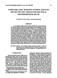
FIG. 1. Interface discretization by triangles with vortices 䊊. The basic surface element S j is defined by the centers of mass of the triangles 共䊐兲 and element sides 共䊏兲 to which the node x j belongs.

冕

Sc

⫺

G共 x0 ,x兲 •ns 共 x兲 ds 共 x兲 ⫽0,

冕

Sc

共7兲

T共 x0 ,x兲 •ns 共 x兲 ds 共 x兲

再

8␲,

⫽I 4 ␲ , 0,

if x0 inside S c if x0 on S c if x0 outside S c

冎

III. NUMERICAL METHOD

共8兲

,

which hold for an arbitrary closed surface S c , where ns (x) is the unit normal to S c directed outwards. Based on 共7兲 and 共8兲, it was proven19 that the single- and double-layer potentials on a part D of the interface can be expressed as integrals over its contour ⳵ D,

冕冕

D

G共 x0 ,x兲 •nD 共 x兲 ds 共 x兲 ⫽

D

T共 x0 ,x兲 •nD 共 x兲 ds 共 x兲 ⫽2

冖冖

dy⫻y ; ⳵ D 兩 y兩

共9兲

y共 y⫻dy兲

⳵D

兩 y兩 3

冉冖

⫹2I C⫹

The main advantage of the contour representations 共9兲 and 共10兲 is that they are nonsingular. This is obvious for the single-layer potential. For the double layer 共10兲 this can be seen projecting the contour ⳵ D on the unit sphere centered at x0 , see section 3.2 of Bazhlekov.19 The nonsingularity of the last integral in 共10兲 is achieved by a proper choice of the vector a (a⫽⫺y/ 兩 y兩 ,y苸 ⳵ D). These steps are used in Sec. III D to improve the accuracy of the contour-integral calculation, see Eq. 共20兲. A nontrivial situation can appear when x0 →x⬘0 苸 ⳵ D. This is not related, however, to a singularity of the integrals, but to the uniqueness of the projection of x0 苸 ⳵ D on the unit sphere and can be easily overcome. In the present numerical method such situation (x0 苸 ⳵ D) cannot happen and the unit-sphere projection of ⳵ D is always well defined. Other advantages of the contour representations 共9兲 and 共10兲 are that their implementation for nonclosed interfaces is direct and they involve integration on a curve instead of on a surface. In addition, the precise knowledge of the normal vector nD is not necessary for the calculation of the layer potentials. By applying the contour integration on the elements of a partitioning of a closed interface, the identities 共7兲 and 共8兲 are satisfied exactly, regardless of the accuracy of the calculation of the contour integrals.

冊

a• 共 dy⫻y兲 , ⳵ D 兩 y兩共兩 y兩 ⫹a"y 兲共10兲

where y⫽xˆ⫽x⫺x0 ; x苸 ⳵ D and a is an arbitrary unit vector. In the above equations, dy⫽t dl(y), where t is the unit vector tangential to the contour ⳵ D defined as t⫽b⫻n, see Fig. 1. The absolute value of the sum in the brackets of 共10兲 has to be equal to the solid angle ␻ (x0 ,D), defined by the pole x0 and D, and its sign depends on the direction of the normal vector nD (x). The last integral in 共10兲 is a measure of the solid angle ␻ a (x0 , ⳵ D) defined by the pole x0 and the contour ⳵ D to which the ray A x⫺a ⫽ 兵 x0 ⫺ ␣ a; ␣ ⬎0 其 does not 0 belong. In general, there are two solid angles defined by x0 and ⳵ D. Thus, the constant C accounts for the difference between ␻ (x0 ,D) and ␻ (x0 , ⳵ D): if x0 苸D, then C⫽⫺2 ␲ sign(a"n(x0 )); if A x⫺a crosses D in a point AD , 0 then C⫽⫺4 ␲ sign(a"n(AD )).

The main elements of the numerical method such as the calculation of the velocity field given by the boundary integral formulation 共6兲 and the evolution of the interfaces via a time integration scheme are discussed here. A. Interface discretization and mesh refinement

The initially spherical interfaces are triangulated by flat triangles.10 Each triangular phase of an icosahedron inscribed in a sphere is subdivided into n 2 equal triangles, whose vertices are projected onto the sphere. This triangulation consists of N⫽20n 2 flat triangles and is optimal for a closed interface topology: N/2⫺10 vortices have coordination number N c ⫽6 and 12 vortices with N c ⫽5. Based on this triangulation, the interface is discretized by surface elements S j corresponding to the nodal points x j of the mesh. Every element S j is composed by 1/3 of the triangles to which x j belongs, see Fig. 1; S j are the basic surface elements where the curvature and the boundary integrals are calculated. In addition, the mesh properties are optimized in three ways. 共i兲

Element size optimization:10 for a fixed mesh topology the nodes are additionally moved with the extra tangential velocity w(x,t), see 共5兲. This velocity is determined on the base of the local characteristics of the mesh and the interfaces, such as element size, curvature k and the distance to the closest interface h, w共 xi 兲 ⫽ 共 I⫺nn兲

冉兺 j

关 a⫹b 共 h 共 x j 兲兲 ⫹c 兩 k 共 x j 兲兩 3/2兴

冊

⫻ 共 x j ⫺xi 兲 ⌬S j ⫺u共 xi 兲 ⫹us ,

共11兲




1067

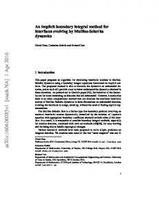
to unwanted large or small angles, see Figs. 2共c兲 or 3共e兲. An optimization of the coordination number can be easily achieved by reconnecting the nodes in two neighboring triangles. Such an example is shown in Fig. 2共c兲, where the dashed–dotted edge is replaced by the dashed one. From this figure is seen that this reconnection optimizes locally the coordination numbers from 共8,4,7,5兲 to 共7,5,6,6兲. For meshes used in the present study the coordination number N c is always in the interval 5 ⭐N c ⭐7.

FIG. 2. Schematic sketch of subtraction 共a兲 and addition 共b兲 of edges 共nodes and elements兲, and reconnection of nodes 共c兲.

where the summation involves only the nodes x j that are directly connected to xi ; us is an average velocity of the interface to which xi belongs. The term ⫺u(xi ) ⫹us in 共11兲 eliminates a mesh distortion due to the tangential component of the hydrodynamic velocity u. The constant c controls how fine the mesh is in the high curvature regions. The function b depends on the problem under consideration: in the case of drop-to-drop interaction the mesh is required to be finer in the film regions, thus b(h)⫽const h⫺1; in the case of foam-drop dynamics b(h)⫽const h and in this way the mesh is maintained finer in plateau borders and junctions, where the curvature and h have larger gradients. For these two types of problems we use only the mesh size optimization in the simulation. In the case of drop deformation good mesh properties cannot always be achieved only through element size optimization and a change in the topology is necessary. 共ii兲 Subtraction and addition of edges according to a criterion for the proper edge length,4,24 l0j ⫽max共min共lmax ,const k⫺1 j 兲,lmin 兲,

共12兲

where k j is a local curvature;24 l min and l max are given in advance and denote the global minimal and maximal edge lengths. Thus, if the length of an edge l j is smaller than l 0j •3/4, the edge is removed,22 as is shown in Fig. 2共a兲. The edge subtraction is followed by addition of edges:25 if for a given edge, l j ⬎l 0j •3/2, it is split into two by adding the middle point, marked by 共䊊兲 in Fig. 2共b兲. Then every triangle with split edges is subdivided into two, three, or four triangles depending on the number of edges which are split, as shown in Fig. 2共b兲. 共iii兲 Topology optimization: After edge subtraction and addition the coordination number of some nodes can deviate substantially from the optimal (N c ⫽6). This leads

The standard scheme for mesh refinement involving a change of the mesh topology is as follows, see also Figs. 3共a兲–3共d兲: subtraction and addition of element edges followed by topological optimization and finally element size optimization in combination with a projection of the nodes on the initial interface. A comparison between Figs. 3共d兲 and 3共e兲 demonstrates how useful the topological optimization can be. A disadvantage of the local element-size optimization 共11兲 is the stability constrain, which can be much tighter than that of the passive stabilization algorithm.17 However, the present approach is more flexible for mesh refinement in high curvature regions or near contact zones. Moreover, it can be directly extended to take into account other important characteristics, such as high gradients of the surfactant concentration or the temperature. In addition, the time integration scheme, proposed in Sec. III E, overcomes the difficulties due to the poor numerical stability of the local element-size optimization 共11兲. B. Curvature calculation

The mean curvature k(x) and the normal vector n共x兲 for the surface element S j are computed by means of a commonly used formula, see for instance10 k 共 x j 兲 n共 x j 兲 ⌬S j ⬇

冕

Sj

k 共 x兲 n共 x兲 ds⫽⫺

冖

⌫j

b dl,

共13兲

where ⌫ j ⫽ ⳵ S j is the contour of S j and b is the unit outward normal to ⌫ j vector lying in the plane tangential to S j , see Fig. 1. Different possibilities for the choice of S j exist. 共a兲共b兲

Loewenberg and Hinch10 defined ⌫ j by the bisectors of the triangle edges surrounding the vertex x j . In the present study S j is the basic element for the node x j , as defined in the preceding section, see also Fig. 1.

The most popular test for the accuracy of a curvature calculation is the following:17 for an analytically given interface shape the mesh nodes are projected on the interface and the numerically calculated curvature is compared with the analytical one. According to this test, the curvature calculated by 共13兲, where S j is chosen as in 共b兲, does not converge even for uniform meshes on a sphere. In the nodes with N c ⫽5 the error is about 14%, independently of the number of elements. It is our opinion, however, that according to 共6兲 a spherical 共nondeformed兲 interface is one which has constant curvature. Indeed, for a given mesh in the absence of


1068



FIG. 3. An example of a mesh refinement that involves topological changes 共a兲 the mesh before refinement; 共b兲 after subtraction and addition of edges; 共c兲 after topological optimization; 共d兲 final mesh, after mesh size optimization 共relaxation兲; 共e兲 as 共d兲, however, without topological optimization.

any external flows or forces, the drop would relax to a shape for which the curvature in all nodes will be equal, independently of the way of curvature calculation. Then, by comparing the relaxed interface with the equivalent sphere, a conclusion for the accuracy of the curvature calculation can be drawn. According to this test the present method of curvature calculation converges for a sphere and has a second-order accuracy, which is seen in Fig. 4. Similar tests can also be designed for nonspherical interfaces.17 Zinchenko et al.17 have proposed an approach for the calculation of the curvature and normal vector, which is based on a local paraboloid fitting. We find their approach very efficient and more accurate than the contour integration 共13兲. An advantage of the present method, however, is that it provides an average curvature in S j , which is consistent with the calculation of the boundary integrals on S j . In other methods10,17 the calculation of the boundary integrals has a second-order accuracy only for uniform meshes. For nonuni-

FIG. 4. The maximal deviation of relaxed 关according to 共6兲兴 drop with equivalent radius 1 from unit sphere for different meshes. N is the number of mesh nodes.




xlp ⫽R l 共 x⫺Ol 兲 / 兩 x⫺Ol 兩 ,

l⫽1,2,3.

1069

共15兲

共3兲 The projection of the node x on the higher-order interface approximation S p is defined by means of the linear combination, 3

兺 w l •xlp .

x ⫽ p

FIG. 5. Schematic 2D version of the higher-order approximation of the interface 共thicker curve兲. It is constructed based on the initial discretization 共thinner lines兲 and the circuits C j (O j ,R j ) 共dashed lines兲.

l⫽1

共16兲

The coefficients w l are functions of the distances from x to the vertices and edges of the triangle and can be defined to be continuous across the edges, l

w l⫽ form meshes the integration deviates from the trapezoidal rule and loses the second-order accuracy. In the case of drop-to-drop interaction we compared the two approaches for curvature calculation 共13兲, based on the choices 共a兲 and 共b兲. The results were identical for relatively uniform meshes, however, for nonuniform meshes approach 共a兲 led to numerical instabilities, while approach 共b兲 still supplied stable results. It is worth to mention that the contour integration 共9兲 and 共10兲 of the layer potentials does not include the normal vector. Thus, in the present method the normal vector appears only in the element size optimization 共11兲 and the higherorder interface approximation, presented in the following section. This makes our method less sensitive to errors in the normal vector calculation.

兺

k⫽l⫺1

w kl w k⫹1 w k⫺1 /w,

where k and l correspond to the local numeration of the sides and the nodes in the triangle 关the lth node belongs to the (l⫺1)th and lth sides兴; w k is the distance 兩 x ⫺yk 兩 , where yk is a projection of x on the kth side (w 0 ⫽w 3 ; w 4 ⫽w 1 ); and w kl ⫽ 兩 x j ⫺yk 兩 / 兩 xl ⫺x j 兩 correspond to the linear description of yk on the kth side 共the jth and lth nodes are the vertices of the kth side兲. Finally, w is defined as 3

w⫽

兺

w k w k⫹1 ,

k⫽1

which automatically leads to 3

兺 w l ⫽1.

l⫽1

C. Higher-order approximation of the interfaces

The reason for the construction of a higher-order interface approximation arose from the simulations of foam-drop dynamics, see Sec. IV D. A typical feature of a foam structure is the presence of film regions, where the interface-tointerface distance h can be a few orders of magnitude smaller than the drop size. The main problem arises from the disjoining pressure in 共3兲, where small disturbances in the value of h can introduce a significant inaccuracy to the calculation of the interfacial forces and lead to continuously growing numerical instabilities. In the case of monodispersed foams, because of the flat film regions, the initial interface approximation can provide sufficient accuracy. For polydispersed foams the film regions have, in general, nonzero curvature and a better approximation of the interfaces is necessary. To improve the accuracy of the calculation of h(x) we propose a higher-order approximation of the interfaces. It is based on the initial triangulation by linear triangles and information about the curvature and the normal vector in the nodal points. It is constructed following the next scheme, for illustration see the two-dimensional example in Fig. 5. 共1兲 A sphere C j (O j ,R j ) is associated with every nodal point xj , R j ⫽ 兩 k 共 xj 兲兩

⫺1

,

O j ⫽x j ⫺n共 x j 兲 /k 共 x j 兲 .

共14兲

共2兲 Node x of the triangle with vertices (x1 ,x2 ,x3 ) is projected radially on the sphere C l ; l⫽1, 2, 3, see Fig. 5,

Different possibilities exist for the projection yk of x on the edges. In the present study we use the orthogonal one. Apparently, when x is on an edge of the mesh, the coefficients w l are those from the linear description of x on the edge. Thus, the approximation S p of the interface S is globally smooth and its curvature is globally continuous. The interface-to-interface distance h p (x) calculated on the base of the higher-order interface approximation is also globally smooth and is directly related with the curvature via 共14兲. A disadvantage of the approximation S p is that it is based on a local fitting with spheres, which is not appropriate in the general case of a nonspherical surface. Zinchenko et al.17 developed an efficient method for local paraboloid fitting for the curvature and normal vector calculation. We expect that a significant improvement of the interface approximation can be achieved simply by replacement of the projection on the sphere in step 共2兲 above with that on a paraboloid. We found, however, that the approximation presented here is sufficient for the simulation in Sec. IV D, where the interfaces in the film regions are well approximated locally by spheres, see Fig. 6. D. Boundary integral calculation

One of the most important aspects of a boundary integral method is the calculation of the integrals in 共6兲. Applying the mean value theorem on the surface elements S j , the boundary integrals can be approximated as


1070



FIG. 6. Comparison of the initial interface approximation by flat triangles 共solid line兲 with the higher-order one 共dashed lines兲. Zoomed film region from Fig. 18共c兲 is shown.

冕

S

f 共 x兲 G共 x0 ,x兲 •n共 x兲 ds 共 x兲 ⫽

冕

S

兺j

f 共 xj兲

冕

Sj

G共 x0 ,x兲 •n共 x兲 ds 共 x兲 ⫹O 共 ⌬x 2 兲 ,

共17兲

u共 x兲 •T共 x0 ,x兲 •n共 x兲 ds 共 x兲 ⫽

兺j u共 xj兲 • 冕S T共 x0 ,x兲 •n共 x兲 ds 共 x兲 ⫹O 共 ⌬x 2 兲 ,

共18兲

j

where f (x j ) and u(x j ) are average values on S j . The integrals on the right-hand side of 共17兲 and 共18兲 are calculated by means of the contour integrations 共9兲 and 共10兲. In the present method the contour ⌫ j is a polygon, ⌫ j ⫽艛 i ⌫ ij ⫽艛 i 关 yi ,yi⫹1 兴 , see Fig. 1, and 共9兲 and 共10兲 read19 I Gj 共 x0 兲 ⫽ ⫽

冕冕

Sj

G共 x0 ,x兲 •n共 x兲 ds 共 x兲

dy⫻y ⫽ ⌫ j 兩 y兩

冏

⫻log

FIG. 7. The relative error 储 I Q ⫺I Qex储 / 储 I Qex储 , where I Q is calculated by three different methods. Q stands for 共a兲 G and 共b兲 T. The norm of the exact solution 储 I Qex储共thicker lines兲 is not given in %.

兺i 兩 yi兩 sin共 ␤ i 兲

冏

共 1⫹cos共 ␤ i 兲兲 • 共 1⫹cos共 ␥ i 兲兲 yi ⫻yi⫹1 • i i⫹1 sin共 ␤ i 兲 •sin共 ␥ i 兲兩 y ⫻y 兩

共19兲 and I Tj 共 x0 兲 ⫽

冕

Sj

⫽2

⫽2

T共 x0 ,x兲 •n共 x兲 ds 共 x兲

冖

y共 y⫻dy兲

⌫j

兺i

兩 y兩

3

冉冖

⫹2I C j ⫹

a• 共 dy⫻y兲兩 y 兩 • 共兩 y兩 ⫹a•y兲 ⌫j

冊

共i兲

共 zi ⫹zi⫹1 兲共 zi ⫻zi⫹1 兲

冋

⫹2I C j ⫹

冋冋

⫻ arctan

共ii兲

1⫹zi "zi⫹1

兺i

2a• 共 zi ⫻zi⫹1 兲 g i 兩 zi ⫻zi⫹1 兩

In order to check the validity of the contour-integral representations 共19兲 and 共20兲 we performed the following numerical test. Consider a surface element S j , see Fig. 1, from a discretization (⌬x⬇0.025) of the unit sphere centered at the origin. The integrals I Qj 共Q stands for G or T兲 are calculated both by 共19兲 and 共20兲, and as surface integrals. The surface integration 共dashed lines in Fig. 7兲 is based on

册

冋册册册

ei 共 1⫺ f i 兲 •tan共 ␣ i /2兲 ⫹e i ⫺arctan gi gi

a commonly used6,17 one-point integration rule, I Qj ⫽⌬S j Q(x0 ,x j )•n(x j ), where the exact value for the normal vector, n(x j )⫽x j , is taken, subdivision of every triangle (x j ,yi ,xi⫹1 ), see Fig. 7, into N 2t equal triangles. Then the above one-point integration rule is applied to every subtriangle after its vertices and mass center 共the integration point兲 have been projected on the unit sphere and for the normal vector the exact value is taken.

,

共20兲 where zi ⫽yi / 兩 yi 兩 ; e i ⫽ 关 cos(␪i⫹1)⫺cos(␪i)•cos(␣i)兴/sin(␣i); f i ⫽cos(␪i) and g i ⫽ 冑1⫺e 2i ⫺ f 2i . The constant C j depends on the position of the pole x0 and the direction of the vector a with respect to the surface element S j as described in Sec. II C. The angle ␣ i is determined by the vectors zi and zi⫹1 , and ␪ i by a and zi .

The results are compared in Fig. 7 with the exact soluex , obtained by the contour integration 共9兲 and 共10兲 tion I Q applied for the projection ⌫ pj of ⌫ j on the unit sphere. In the present test the pole x0 moves radially towards the point y1 ⫽(x j ⫹xl )/2, where xl is a node directly connected to x j , see Fig. 1. Thus, the horizontal axis, 兩 x0 兩 ⫺1, in Fig. 7 corresponds to the distance pole interface. Figure 7 shows that when the number of the integration




points N 2t increases, then the surface integrals converge to ex , which indicates the validity of the the exact values I Q contour-integral representations 共9兲 and 共10兲. It is also seen that for a distance pole interface of about 0.01, the one-point integration has more than 10% error. In contrast, when the contour integration is used the error is less than 0.1%, independently of the distance pole interface 共the error did not increase even at 兩 x0 兩 ⫺1⫽ 兩 x0 ⫺y1 兩 ⫽10⫺7 ). This also indicates the nonsingularity of the contour integration 共note that y1 苸 ⳵ S j ). For relatively large distance pole-interface 共for instance 兩 x0 兩 ⫺1⬎0.2) both, surface and contour, integrations have comparable accuracy. The main disadvantage of the contour integration 共19兲 and 共20兲 is that it involves intrinsic functions that slow down the performance of the method. Compared with the one-point surface integration, the contour integration is an order of magnitude slower. To improve the performance of the method, the exact formulas 共19兲 and 共20兲 are used only for S j that are close 共two layers of elements兲 to x0 . For the rest of the interface the contour integrals are calculated by means of two-point integration rule applied to every segment of the contour ⌫ j . This procedure improves the performance about twice, but it is still 5– 6 times slower than the surface integration. We think, that a significant improvement could be achieved if the contour integration in a vicinity of x0 is combined with the surface integration on the rest of the interfaces. E. Multiple step time-integration scheme

A well-known difficulty during the simulation of free boundary problems is the numerical instability due to the surface tension. Such instabilities limit the time step and thus slow down the performance, especially for small capillary numbers and small element size. An estimate for the time step required for a stable solution is6,17

⌬t⬍O 共 Ca min共 ⌬x兲兲 ,

共21兲

where min共⌬x兲 is the minimal element size. In addition, the disjoining pressure A/h 3 as well as the element-size optimization 共11兲 can further limit the time step. To overcome this difficulty an idea is used here, which is based on the following two facts. First, the above-mentioned numerical instabilities are local, i.e., the instabilities in a node x j from the interface are mainly due to the time discretization of f (x) in the nodes that are in a close vicinity of x j 共denote the set of these nodes by N j ). Second, the calculation of f (x) and w共x兲 requires O(N) operations, while for the boundary integrals they are O(N 2 ). The idea is when the velocity at x j is calculated, we refresh the values corresponding to nodes in N j at every time step ⌬t and all other values—after M such time steps. The extra tangential velocity w共x兲 is also calculated at every time step. To illustrate this idea, the boundary integral formulation 共6兲共after discretization兲 is rearranged as follows:

共 ␭⫹1 兲 u共 x j 兲 ⫽⫺

1071

␭⫺1 u共 xi 兲 •ITi 共 x j 兲 4 ␲ i苸N

兺

冉

⫺

1 i f 共 xi 兲 IG 共 x j 兲 ⫹ 2u⬁ 共 x j 兲 4 ␲ i苸N j

⫺

1 i f 共 xi 兲 IG 共 xj 兲 , 4 ␲ i苸N j

兺兺

冊

共22兲

where N denotes the set of all nodes and N j ⫽N/N j . In the present method only the terms f (xi ) and u⬁ (x j ) in the brackets in 共22兲, are calculated at every time step ⌬t, which requires O(N) operations. The other terms on the right-hand side of 共22兲 are kept unchanged for M time steps. Their calculation requires O(N 2 ) operations and is performed once within every time interval ⌬T⫽M ⌬t. Thus, the total number of operations for a time interval of length ⌬T is O(N 2 ⫹M •N). For the standard iteration scheme,6,17,18 where all terms on the right-hand side of 共22兲 are calculated at every time step ⌬t, the corresponding number of operations is O(M •N 2 ). Thus, for M ⰆN the proposed time integration scheme is about M times faster than the standard one. An estimate for an optimal value of M can be obtained comparing the contribution to the total error of that due to the time integration with that due to the spatial discretization. The total error can be estimated as O((M •⌬t) 2 ) ⫹O(max(⌬x)2). Taking into account 共21兲, a comparison between the two terms in the total error leads to M ⬇O(max(⌬x)/(Ca min(⌬x)). For a number of problems, for instance at small Ca and highly nonuniform meshes, M can have a significant value. Other examples are steady-state problems as well as those with small time gradients, where the total error is dominated by the error due to the spatial discretization. In such cases the time step usually is limited by a condition for numerical stability, e.g., 共21兲, and can be much smaller than that necessary for an accurate solution. To demonstrate how the performance and the accuracy depend on the value of M (⌬T), we consider the following test problem: deformation of an initially spherical drop of radius R and viscosity ␮ in a planar extensional flow (u 1 ⫽Gx 1 ; u 2 ⫽⫺Gx 2 ; u 3 ⫽0) in the time interval 关0;0.2兴 at Ca⫽ ␮ GR/ ␴ ⫽0.05, the case ␭⫽1 is considered for simplicity. The drop deformation in the considered time interval is shown in Fig. 8. A relatively large gradient of the deformation is observed, which is an indication of the relevance of the test 共for steady problems the present scheme would not introduce any additional error, independently of the value of M兲. A mesh of 10 580 triangular elements was used at time step ⌬t⫽2.5⫻10⫺4 , which is an order of magnitude smaller than the stability limit 共21兲. The simulations for different values of M ⫽2 l ; l⫽1,2,...,10 were performed and compared with the standard scheme (M ⫽1). The relative extra 共due to the proposed scheme兲 error in % for the drop deformation at t⫽0.2 is shown in Fig. 9. A linear dependence of the performance on M is also seen 共䊊兲. For instance, at M ⫽256 the performance of the present scheme corresponds to that of the standard time integration at time step about 0.064, which is 10 times larger than the stability limit. Thus, for the test problem considered here, the present time integration


1072



where the matrix A T corresponds to the double layer operator, after it has been deflated.15 The vector b G takes into account the single-layer potentials and the external flow as well. At every big time step M •⌬t all elements of A T and b G are calculated and then successive iterations k⫽0,1,2,... are performed. At the small time steps m•⌬t, m⫽1,2,...,M only a part of b G is recalculated and iterations are performed if b G differs significantly from the corresponding value when the last iteration process has been performed. Thus, if the previous iterations of 共23兲 have been performed at small time step m 1 ⬍M and if

冋兺

册

m2

max j

FIG. 8. Drop deformation in a planar extensional flow. B⬍W⬍L are the three lengths of the drop—along x 1 , x 3 , and x 2 axes, respectively.

scheme at ⌬T⫽0.064 is an order of magnitude faster than the standard one, and introduces an extra error less than 0.5%. The performance and the error are determined by the large time step ⌬T and are almost insensitive to the values of ⌬t and M ⫽⌬T/⌬t, provided M ⰆN. The present scheme is stable even at ⌬T⫽0.25 (M ⫽1000), however, the accuracy is unacceptable. For the simulations in the present study, time steps ⌬t several times smaller than the stability limit were used with M of the order 100. Thus, in most of the cases the CPU time determining time step ⌬T was about an order of magnitude larger than the stability limit 共21兲. The set N j consists of the node x j , the node xl closest to x j that belongs to another interface and the nodes directly connected to xl as well. The algebraic system 共22兲 is solved by the method of successive substitutions.6,16 To demonstrate how this is done in combination with the multiple step time-integration scheme, the system is written in the form k⫹1

u

共 t 兲 ⫽u 共 t 兲 •A T 共 t 兲 ⫹b G 共 t 兲 , k

共23兲

m⫽m 1

兩 b G 共 x j ,t⫹m•⌬t 兲 ⫺b G 共 x j ,t⫹ 共 m⫹1 兲 •⌬t 兲兩 ⬎ ⑀ ,

then successive iterations are performed at time step m 2 ⫺1 as well. Otherwise the solution at time step m 2 is obtained based on the previous step and the difference in b G , i.e., u共 x j ,t⫹m 2 •⌬t 兲 ⫽u共 x j ,t⫹ 共 m 2 ⫺1 兲 •⌬t 兲 ⫹b G 共 x j ,t⫹m 2 •⌬t 兲 ⫺b G 共 x j ,t⫹ 共 m 2 ⫺1 兲 •⌬t 兲 . As a criterion for convergence the standard one is used, 储 uk (t)⫺uk⫺1 (t) 储 ⬍ ⑀ , with a typical value ⑀ ⫽10⫺3 . Zinchenko et al.17 have used a combination of biconjugate gradient iterations and simple iterations, which could be a better alternative. For the problems considered in the following section we found the method of successive substitutions sufficiently efficient: for most of the simulations only 2–3 iterations per big step ⌬T were necessary for convergence.

IV. NUMERICAL RESULTS

To demonstrate the accuracy and stability of the method different problems for deformable interfaces are considered in this section, including challenging problems that involve large curvature or interfaces at very close approach. A. Drop deformation at zero interfacial tension

FIG. 9. Comparisons for the accuracy and performance between the multiple step time-integration scheme and the standard scheme for different value of the parameter M. The extra relative error in % for D(䉭) and C(䊐); the relative CPU time is given by 共䊊兲.

Drop deformation in simple shear and planar extensional flows at zero surface tension Ca⫽⬁ is considered below. This problem was chosen mainly as a test for the calculation of the boundary integrals I Ti and the iterative method 共22兲 at ␭⫽1, as well as a shape-stabilizing procedure given in this section. Recently, Wetzel and Tucker26 presented an analytical model for the deformation of an ellipsoidal drop of zero interfacial tension in a linear velocity field. Comparisons with some of their results are performed here to validate our model for the case of zero interfacial tension. The main difficulty for a direct numerical simulation of such an extreme situation is the loss of the smooth shape of the interface. Indeed, initially small errors due to the discretization of the interface grow continuously because of the velocity gradient.




1073

FIG. 11. Steady shape of a bubble, ␭⫽0, in simple shear flow, u⫽y, at Ca⫽1.25: 共a兲 Side view, in (x,y) plane; 共b兲 top view, in (x,z) plane.

FIG. 10. Comparisons with the results of Wetzel and Tucker 共Ref. 26兲共thick lines兲 and Toose 共1998兲共䊊兲. The present results are given by 共*兲: 共a兲 Drop deformation in simple shear flow for ␭⫽3, the angle between the major axis of the drop and the flow direction is also shown 共dashed line兲; 共b兲 drop deformation in planar extensional flow for ␭⫽18.6.

To overcome this, we propose a shape-stabilizing procedure. It is, in fact, an addition of an extra interfacial velocity based on the local gradient of the curvature, ws 共 x j 兲 ⫽const ⌬S j

兺i 共 k 共 xi 兲 ⫺k 共 xj 兲兲 I Gij共 xj 兲 ,

共24兲

are the contour integrals 共19兲 for the segment where ⌫ i j ⫽ ⳵ S i 艚 ⳵ S j when x0 ⫽x j . In fact, the summation in 共24兲 involves only the nodes i directly connected with j 共for every other node ⌫ i j ⫽0” ). Thus, the extra velocity ws (x j ) in the node x j depends only on the curvature in x j and the neighboring nodes. It is easy to see that if the curvature k is a linear function on the interface around x j , the velocity ws (x j ) would be negligible. In the cases when the curvature has a local minimum or maximum in x j , the extra velocity ws (x j ) can be significant and will smooth the interfaces. The constant in 共24兲 determines the strength of the smoothing and in the present simulation is set to N⫻10⫺3 , at which value ws is small enough to influence the hydrodynamic velocity, but is capable to keep the interface smooth. Figure 10 shows comparisons of our results with Wetzel and Tucker26 and also with the boundary integral method simulations of Toose 共1998兲, as referred in Wetzel and Tucker.26 In Fig. 10共b兲 our results for a finite capillary number Ca⫽1 are also given. They illustrate the applicability of the results of Wetzel and Tucker26 to the case of small but nonzero interfacial tension. Similar agreement was obtained ij (x j ) IG

with the results of Wetzel and Tucker,26 presented in their Fig. 3, regarding drop tumbling for ␭⫽10 and ␭⫽20, and drop widening for ␭⫽0.1. The good agreement with the results of Wetzel and Tucker26 indicates the ability of the present method for simulation of deformable interfaces at zero interfacial tension. The comparisons also show that the shape-stabilizing procedure 共24兲 does not influence the results. Thus, this procedure can be successfully used in the case of nonzero interfacial tension 共finite capillary numbers兲, where the shape stabilization 共24兲 is expected to have less influence on the solution. In the simulations presented in the following sections, however, the interfaces were sufficiently smooth and the procedure was not used. It was used only in some cases as a local shape relaxation procedure, applied after mesh refinement which involves topological changes. B. Drop deformation and breakup at finite interfacial tension

A number of simulations were performed in the case of drop deformation at finite interfacial tension. The first group of simulations concerns steady drop shape in simple shear flow. The comparisons with the steady drop shapes presented by Cristini et al.24 共see their Fig. 3兲 for Ca⫽1.43; ␭⫽3 and Ca⫽0.8; ␭⫽0.01 showed good agreement in the second case: less than 2% relative difference regarding the drop axis ratios. In the first case 共Ca⫽1.43; ␭⫽3兲, however, our results showed about 20% smaller deformation than that of Cristini et al.,24 but are in good agreement with the results of Zinchenko 共private communication, 2003兲. Figure 11 shows the steady shape of a bubble, ␭⫽0 and Ca⫽1.25. Sharp drop edges can be seen in the figure, the situation typical for small drop viscosity with respect to the continuous phase viscosity, ␭Ⰶ1. These results prove the applicability of the presented numerical method for the simulation of bubble deformation that involves high curvature regions 共the curvature at the drop ends is about 50兲 as well as the effectiveness of the mesh adaptation. The other group of simulations concerns transient drop


1074



FIG. 12. Drop breakup in simple shear flow 关 u⫽0.5(x⫹y); v ⫽⫺0.5(x⫹y)] at Ca⫽0.25, ␭⫽10—frames 共b兲–共d兲. Initially, for t⫽0 – 13.65, the drop is elongated in planar extensional flow (u⫽x; v ⫽⫺y)—frames 共a兲.

deformation in different kinds of flows that leads to drop breakup. Good agreement is obtained with the results of Cristini et al.24 for ␭⫽1 presented in their Sec. IV C. Drop deformation and breakup at Ca⫽0.25 and high viscosity ratio, ␭⫽10, is shown in Fig. 12. It is known that at ␭⫽10 the drop will not breakup in simple shear flow unless it has not

undergone a substantial initial deformation.27 Thus, for the simulation presented in Fig. 12 the following protocol for the external flow was used. Starting from spherical shape at t ⫽0 the drop is elongated in planar extensional flow (u⫽x; v ⫽⫺y), frames 共a兲. At time t⫽13.65, when the drop length is about 5.8 from the equivalent drop radius, the flow is



FIG. 13. The evolution of the neck radius, R neck around t⫽21 from the simulation presented in Fig. 12.

switched to a simple shear flow 关 u⫽0.5(x⫹y); v ⫽⫺0.5(x ⫹y)], frames 共b兲. The orientation of the chosen simple shear flow is essential. If, for instance, the standard shear flow, u ⫽y, is applied, the drop will retract without breakup. After the flow is switched to simple shear flow, the drop elongation continues mainly due to the chosen flow direction, see the left frame 共b兲 (t⫽16.05). At this time the drop is already aligned with the flow direction, which is followed by retraction of the drop combined with a necking, see the last frames 共b兲 for (t⫽20, 8 and t⫽21.44). Around t⫽21 the thinning of the neck becomes dominant due to the increasing effect of the surface tension, which indicates that the breakup is imminent, see also Fig. 13. At the end of the simulation, t ⫽21.44, the neck radius is about 2% of the equivalent drop radius. To maintain a sufficient accuracy, the mesh in the neck region is about two orders of magnitude smaller than the maximal element size, see the left frame 共c兲. Following an idea of Cristini et al.,24 the neck is pinched off by splicing of the mesh, the middle frame 共c兲, followed by mesh relaxation 共24兲, the right frame 共c兲. Finally, the two newly formed drops relax towards a steady shape in simple shear flow, see frame 共d兲. The results presented in Fig. 12 demonstrate the possibility of drop breakup in simple shear flow at ␭⫽10, see also Stegeman.27 At ␭⫽1 our simulations always indicate formation of satellite drops during breakup.24,27 For the simulation presented in Fig. 11 our result, however, cannot predict whether a satellite drop will be formed during the breakup. Any further refinement of the mesh in the neck region introduced irregularities on the interface, which 共due to the large curvature兲 led to inaccurate results. C. Drop-to-drop interaction

As an essential part of the coalescence process the dropto-drop interaction is widely investigated.28 One of the main difficulties in the numerical simulation of the process is the presence of a relatively stable liquid film region where the distance between the interfaces is several orders of magnitude smaller than the drop size. In contrast to the neck thinning during the drop breakup, the film drainage between interacting drops can be relatively slow. This means that numerical errors can more easily influence the results for drop coalescence than that for breakup.


1075

For instance, a neck radius of 10% of the drop size already can predict imminent breakup8 共see also Fig. 13兲, while two orders of magnitude thinner film 共0.1%兲 could be insufficient for prediction of film rupture and, subsequently, coalescence. In addition, the small capillary numbers typical for coalescing systems make the numerical simulations of the coalescence process even more difficult and challenging. In order to predict coalescence during drop interaction, the evolution of the film thickness has to be traced to values of the order of the critical film thickness, when the attractive van der Waals forces become dominant leading to film rupture. Most of the existing 3D simulations of drop-to-drop interaction, obtained without restriction on the drop deformation, face significant difficulties to resolve films of thickness less than 1% of the drop radius. The results of Zinchenko et al.17 are the first simulations of films thinner than 1% of the drop radius. Numerical results for much thinner films were obtained28 –31 based on so-called asymptotic theory. In this approach axisymmetric iterations of slightly deformable drops 共film radius much smaller than drop radius兲 are considered, where the film flow is governed by the lubrication equations. Recently, Rother and Davis32 have extended the asymptotic theory to the case of drop-to-drop interaction in linear flows. Here, we compare our results with the predictions of the asymptotic theory, regarding film drainage between drops interacting in simple shear flow. The time step for the numerical simulations of drop-todrop interaction is chosen, as in Zinchenko et al.,17 to de1/2 . Here, pend on the minimal film thickness, ⌬T⫽⌬T 0 h min however, the optimal initial time step ⌬T 0 is taken to guarantee numerical accuracy, while in the standard time integration scheme10,17 it is limited by a stability constrain. This is especially important for the present simulations 共at small capillary numbers兲, where time steps an order of magnitude larger than the stability limit are used. The first group of simulations is for axisymmetric interactions of two equal drops in compressional flow at Ca ⫽0.05, see Fig. 14共a兲. The 3D simulations were performed using nonuniform meshes, see Fig. 14共b兲. The time step ⌬T 0 ⫽0.1 共the stability limit is about 0.01兲 was used with M ⫽100. For ␭⫽1 three different meshes were used, in order to check the convergence with respect to the space discretization. The results for the evolution of the center and minimal film thickness are shown in Fig. 14共c兲. The mesh of 2000 elements per drop was insufficient to supply accurate results for the minimal film thickness below 0.003 of the drop radius, while the other two meshes give almost identical results. They are also in agreement with the predictions of a version of the present code for axisymmetric problems. In Fig. 14共d兲 the film profiles are compared at minimal film thickness h min⫽0.0025. A comparison with the asymptotic theory for the results presented in Fig. 14 was not possible due to the large film radius 共0.4兲 and externally driven recirculation within the drops, which influences the film drainage. In this case the recirculation flow inside the drop completely stops the film drainage leading to stationary long-time configuration. This phenomenon has been observed for the first time by Cristini et al.24


1076



FIG. 14. Drop-to-drop interaction in axisymmetric compressional flow (u ⫽0.5x; v ⫽⫺y; w⫽0.5z) at Ca ⫽0.05. The drops are initially spherical and centered at 共0:0;⫾1.5兲: 共a兲 side view and 共b兲 view from the film side of one of the drops at t⫽20 for mesh of 3920 elements per drop; 共c兲 the evolution of the film thickness in the center and the minimal film thickness for three different meshes; 共d兲 film profiles 共cross section with plane z ⫽0) at equal minimal film thickness, h min⫽2.5⫻10⫺3 .

In an attempt to extend the simulations presented above to the case of small viscosity ratio 共␭⫽0.1 and ␭⫽0兲 we faced serious difficulties. The results were in good agreement with the predictions of the axisymmetric code for film thickness of about 0.01, however, deviated significantly for smaller h min . Thus, the results for ␭Ⰶ1 in Figs. 5.7– 8 of Bazhlekov19 are not correct for h min⬍0.01. After we checked different sources for the inaccurate results at ␭Ⰶ1, we concluded, that a possible reason could be the combination of the coarse mesh in the rear part of the drops 关see Fig. 14共a兲兴 and Wielandt’s deflation. The elimination of the eigenvalues from the spectrum of the double layer operator leads to ad-

ditional 共uniform expansion and rigid-body motion兲 terms in the boundary integral formulation, see for instance Eqs. 共9兲– 共15兲 of Zinchenko et al.17 The uniform expansion and the rigid-body motion, being integral characteristics of an interface, are influenced by the global error, and thus, transfer it to the interface velocity. In other words, the global error, which is dictated by the error in the coarsest part of the mesh, could effect the interface velocity everywhere. In the case of single drop or drops at relatively large distance, this would have an insignificant effect on the relative position of the interfaces. However, in the presence of interfaces at close approach, it could have a crucial influence on the accuracy of




the calculation of the film thickness. Thus, the simulations of drops in close approach at small or large viscosity ratio require mesh refinement not only in the gap region, which makes them computationally very expensive. To the end of this section the predictions of the present method are compared with that of the asymptotic theory. We consider the formation and drainage of a film between drops interacting in simple shear flow. The drops are equal, initially spherical and centered at 共⫿1.5;⫾0.25;0兲. Each drop interface is triangulated by a mesh of 5120 triangles, and the time step ⌬T 0 ⫽0.05 is chosen 共the stability limit is again an order of magnitude smaller, about 0.005兲. The parameter M is set to a relatively large value, M ⫽200 (⌬t 0 ⫽0.000 25), in order to maintain sufficiently smooth and fast redistribution of the nodes in the gap region. The viscosity ratio is ␭⫽1 and the capillary number is relatively small, Ca⫽0.025, in order to guarantee the validity of the asymptotic theory. In the asymptotic theory the evolution of the film is given by the solution of simplified axisymmetric film-drainage equations29–32 in the gap between the drops. The drop interaction enters as a boundary condition for the film drainage model,31 to take into account the external flow or force. In the present comparison the formula of Hadamar and Rybczinski33 for the force between two spherical drops in simple shear flow is used: F⫽4.34

2/3⫹␭ ␲ ␮ R 2 ␥˙ sin 2 ␤ , 1⫹␭

共25兲

where ␤ is the angle between the line through the drop centers and the flow direction and has to be given. More general and accurate expressions for the interaction force and angles can be obtained.32,34 However, for the present case 共equal drops at ␭⫽1兲 we found expression 共25兲 sufficiently accurate. A larger error, at Ca⫽0.025, can be accumulated during the time integration for the angle ␤ and also due to the choice of its initial value. The main goal of the present comparison is to verify the accuracy of the boundary integral solution in the gap, which corresponds to the film drainage part of the asymptotic theory. Because of that, in order to reduce the influence of the errors from the outer solution, the angle ␤ in 共25兲 is taken from the boundary integral calculation, starting at a drop-to-drop distance which is an order of magnitude larger than that for the film formation. Except for a shift of about 0.2 in time, the agreement between both results presented in Fig. 15 is good, bearing in mind the extremely small interface separation. The agreement between the predictions for the film radius is also good. A more detailed investigation shows that the film profile obtained by the boundary-integral calculations is very close to axisymmetric; deviation less than 1%, even though the interaction is essentially 3D. This agrees with the analyses,30,32 that during 3D drop interactions at small capillary numbers, the film drainage remains axisymmetric. Another quantification of the validity of the inner solution of the asymptotic theory, regarding the assumption for small deformation, follows from the comparison discussed. This comparison indicates that, for a moderate viscosity ratio, the film drainage

1077

FIG. 15. Drop-to-drop interaction in simple shear flow (u⫽⫺y) at Ca ⫽0.025 and ␭⫽1. The drops are initially spherical and centered at 共⫿1.5; ⫾0.25;0兲. The fluctuations of the present results for h min and R film are due to their discrete evaluation—in the nodes of the mesh.

model is valid even when the film radius is about 20% of the drop radius. The local film thickness minimum, at t about 5.8, is due to the disappearance of the dimple during drop separation, predicted also by the boundary-integral calculation.32 Finally, the shift in the time between both simulations presented in Fig. 15 is due to the assumption of small deformation in the asymptotic theory. The drop deformation outside the gap region in the 3D simulation initially accumulates part of the interaction leading to more gentle collision and a delay of the film formation and, subsequently, the whole process. D. Foam-drop formation and its dynamics in simple shear flow

Liquid foams have a highly structured geometry: liquid films, plateau borders and junctions, see Fig. 16. The presence of relatively large interfacial areas and liquids films of several orders of magnitude thinner than the particle size, determines their complex rheological behavior and, consequently, their practical importance. This, however, introduces the main difficulties during the experimental and theoretical investigations of foam dynamics. Thus, most of the numerical investigations are limited to 2D foams or 3D dry-film foams.35,36 In the dry-film models, films with zero thickness are considered and modelled as mathematical surfaces, neglecting the film drainage and interfacial effects. To our knowledge, the simulations of Loewenberg, de Cunha, Blazwdziewich, and Cristini 共1999兲, as referred by Kraynik and Reinelt,35 are the first for 3D wet foams. They are restricted, however, to the monodisperse case and then only to the formation of the foam during uniform expansion in the absence of external flows. In the present section we consider a foam-drop: a compound drop that consists of several inner drops at high volume fraction completely covered by another immiscible liquid. Such a drop has all structural elements of a polydispersed foam: liquid films bounded by interfaces of significant curvature, plateau borders and junctions, see Fig.


1078


FIG. 16. Foam-drop structure, four inner drops at 95% volume fraction. The film regions 共made transparent兲 are connected via plateau borders, joined in junctions.

16. Simple shear flow is considered here as an example of external flow. For simplicity, the surface tension coefficients for all of the interfaces are assumed equal, ␴, and the viscosities of all liquids equal to ␮. Thus, the problem has two dimensionless hydrodynamic parameters: the capillary number Ca⫽ ␥˙ •R• ␮ / ␴ 共R is the equivalent radius of the foamdrop兲 and the dimensionless Hamaker constant, A, see the discussion after Eq. 共3兲. The disjoining pressure in 共3兲 is very important for the film and thus for the foam stability. Here it is modelled, following Kraynik and Reinelt,35 as ⫺A/h 3 (x). In Fig. 17 a foam-drop formation is shown, the first three pairs of frames 共a兲–共c兲. The first column shows the outer interface and the second, the inner-drop interfaces. Initially the drops are spherical, the outer drop has radius R, the eight equal-size inner drops of radius 0.3R, frames 共a兲 of Fig. 17. The inner drops are then subjected to a nonuniform expansion, where the expansion rate depends on the distance to the closest interface uexp(x j )⫽const n(x j )•h(x j ). When the relative volume of the inner drops reaches 95%, the expansion stops and the interfaces relax. Thus, at time t⫽12.4, frames 共c兲, the foam-drop with 95% volume fraction 共four inner drops of 13.5% and four of 10.25% relative volume兲 is at equilibrium. After t⫽12.4 the drop is sheared at Ca⫽0.2, frames 共c兲–共e兲, during which the foam-drop deforms in a tumbling-like way.37 Such dynamics is due to the repositioning of the inner drops inside the foam-drop, which is a typical process of the dynamics of foams: the particles change their neighbors, which is related with topological transitions between films, plateau borders and junctions. It is known that a configuration is stable when the films are connected 3⫻3 in plateau borders, and the plateau borders are connected 4⫻4 in junctions, which is the case in Fig. 16. Let us follow the evolution of the four front 共upper兲 inner drops in frames 共c兲–共e兲 of Fig. 17. Initially, the left and right drops are separated by the other two drops, which are in


contact—there is a liquid film between them, see frames 共c兲. During the shearing, however, this film disappears leading to a plateau border 共connecting four films兲 between the four drops under consideration, see frames 共d兲. A junction connecting five plateau borders 关four of which are seen on left frame 共d兲 and the fifth is that between the four drops兴 is also formed. Thus, this metastable configuration changes to a stable one, where the initially separated drops are now in contact, forming film between them, and the other two drops separate, see frame 共e兲. The process of drop repositioning can be also seen in Fig. 18, where cross sections in a plane, fitted with the centers of the four drops, are shown at different time instances. Thus, the discussed simulation has not only the main structural, but also the dynamic elements of polydispersed foams. The simulation presented here was performed using 8820 triangular elements on the outer interface and 3380 elements per every inner drop—35 860 elements in total. The mesh is kept finer 共⌬x⬇0.01兲 in the plateau border and junction regions, where the gradients of the curvature and interface-to-interface distance are larger. In the film regions, of almost constant thickness, the edge size is an order of magnitude larger 共⌬x⬇0.1兲. To maintain such mesh properties during the whole dynamics, only mesh-size optimization was used, without topological changes. The minimal film thickness is about 2.5⫻10⫺3 , and as it was mentioned above, the interfaces in the film regions are discretized by elements with two orders in magnitude larger size. In addition, some of the film regions have a significant curvature (k⬇3). Thus, the use of the higher-order interface approximation presented in Sec. III is essential, see Fig. 6. For comparison, when the initial approximation of the interfaces by flat triangles was used, we managed to expand the inner drops only to about 60% volume fraction 关slightly before frame 共b兲兴. The results presented in Fig. 17 were obtained for about three days on Risc 10K 225 MHz single processor. The time step was ⌬t⫽10⫺5 , which was sufficient to obtain numerically stable solution. The limitation on the time step is mainly due to the disjoining pressure term, proportional to h ⫺3 (x) 关 h(x)⬇2.5⫻10⫺3 in the film regions兴. The parameter M in the multiple step time-integration scheme was taken M ⫽1000. For this value the most CPU time consuming single layer potential was calculated only once at every time interval ⌬T⫽10⫺2 . Finally, the higher accuracy due to the contour integration is also very important for the presented simulation of the foam-drop dynamics, mainly due to the presence of interfaces in an extremely close approach and the high gradient of the normal vector in the plateau border regions. The main goal of the simulation presented here was to demonstrate the numerical stability of the method in the presence of disjoining pressure in film regions with significant curvature. A direct and practically important extension of the present simulation can be made by an incorporation of triply boundary conditions.9,10 Recently, Zinchenko and Davis11 made significant improvement in this direction, considering up to 200 drops per periodic box at 55% volume fraction.




1079

FIG. 17. Expansion of the inner drops at constant volume of the whole foam-drop at A⫽2.5⫻10⫺6 共a兲–共c兲. The relative volume of the inner drops is 共a兲 22%; 共b兲 77%; 共c兲 95%. Foam-drop deformation in shear flow at Ca⫽0.2 and A⫽2.5⫻10⫺6 共c兲–共e兲.


1080


FIG. 18. Cross sections of the foam drop at different time instances.

V. CONCLUDING REMARKS

A three-dimensional boundary-integral method is presented for deformable drops in viscous flows at low Reynolds numbers. The main advantage of the method is the calculation of the boundary integrals, based on a contourintegral representation of the single and double-layer potentials. Due to the nonsingular formulation, the contour integration offer a higher accuracy in the vicinity of the singular point, compared with the standard surface integration. Far from the singular point both integrations show comparable accuracy. The main disadvantage of the contour integration is that its performance is about an order of magnitude slower. Thus, an improvement could be achieved, combining the


contour integration around the singular point with surface integration in the rest of the interfaces. Another advantage is that the contour integration, in contrast with the commonly used near singularity subtraction, can be directly applied for nonclosed interfaces. Typical examples in this case are the problems involving three-phase contact lines, which will be a direction of our future efforts.19 In addition, the normal vector is automatically accounted in the contour-integral representation, which makes the results less sensitive to the errors due to the normal vector calculation. The time integration in the present method is stabilized by the proposed multiple step scheme. The scheme offers a solution of the well-known problem of numerical instabilities due to the surface tension. The stabilizing effect of the multiple time-step integration is also important for simulations that involve repulsive van der Waals forces, mainly because of their strong dependence of the film thickness. In addition, the proposed time integration overcomes the numerical instabilities due to the mesh-size optimization technique based on the local grid tension method. The higher-order interface approximation plays an essential role in the accurate calculation of the interface-tointerface distance, especially in film regions with significant curvature. It is important not only for an accurate calculation of the disjoining pressure, but also for a numerical stability during the simulation of polydispersed foam dynamics. An improvement of the present variant of the interface approximation can be easily achieved by making use of the local paraboloid fitting procedure.30 In Sec. IV we present simulations of multiphase problems that involve regions of a high interface curvature and small interface-to-interface distance as well as a strong influence of the capillary and disjoining pressure. The simulations of drop-to-drop interaction show a good accuracy for film thickness of about 0.2% of the drop radius in the case of matching viscosities, ␭⫽1. However, at small viscosity ratio, ␭⭐0.1, the results were inaccurate for film thickness below 1% of the drop radius. We think, that in the case of contrast viscosities, ␭Ⰶ1 or ␭Ⰷ1, the error due to the space discretization becomes global, and is dominated by the error in the coarsest part of the mesh. Thus, the idea of a local mesh refinement in the film region is less attractive in these cases. An important and direct extension of the present method can be made by an incorporation of the effect of an insoluble surfactant.38,39 This, together with an extension applying periodic boundary conditions can make the method an useful tool for a better understanding of the physics within complex multiphase flows. ACKNOWLEDGMENT

This work is sponsored by the Dutch Polymer Institute 共Project No. 161兲. 1

C. Pozrikidis, ‘‘Three-dimensional oscillations of inviscid drops induced by surface tension,’’ Comput. Fluids 30, 417 共2001兲. 2 H. Stone and L. Leal, ‘‘Relaxation and breakup of initially extended drop in an otherwise quiescent fluid,’’ J. Fluid Mech. 198, 399 共1989兲. 3 S. Kwak, M. Fyrillas, and C. Pozrikidis, ‘‘Effect of surfactants on the



instability of a liquid thread. Part II: Extensional flow,’’ Int. J. Multiphase Flow 27, 39 共2001兲. 4 V. Cristini, J. Blawzdziewicz, and M. Loewenberg, ‘‘Drop breakup in three-dimensional viscous flows,’’ Phys. Fluids 10, 1781 共1998兲. 5 V. Cristini, R. Hooper, C. Macosko, M. Simeone, and S. Guido, ‘‘A numerical and experimental investigation of lamellar blend morphologies,’’ Ind. Eng. Chem. Res. 41, 6305 共2002兲. 6 M. Loewenberg and E. Hinch, ‘‘Collision of two deformable drops in shear flow,’’ J. Fluid Mech. 338, 299 共1997兲. 7 A. Zinchenko, M. Rother, and R. Davis, ‘‘Cusping, capture, and breakup of interacting drops by a curvatureless boundary-integral algorithm,’’ J. Fluid Mech. 391, 249 共1999兲. 8 R. Davis, ‘‘Buoyancy-driven viscous interaction of a rising drop with a smaller trailing drop,’’ Phys. Fluids 11, 1016 共1999兲. 9 C. Pozrikidis, ‘‘On the transient motion of ordered suspensions of liquid drops,’’ J. Fluid Mech. 246, 301 共1993兲. 10 M. Loewenberg and E. Hinch, ‘‘Numerical simulation of concentrated emulsion in shear flow,’’ J. Fluid Mech. 321, 395 共1996兲. 11 A. Zinchenko and R. Davis, ‘‘Shear flow of highly concentrated emulsions of deformable drops by numerical simulations,’’ J. Fluid Mech. 455, 21 共2002兲. 12 R. Khayat, ‘‘Three-dimensional boundary element analysis of drop deformation in confined flow for Newtonian and viscoelastic systems,’’ Int. J. Numer. Methods Fluids 34, 241 共2000兲. 13 R. Khayat and N. Ashrafi, ‘‘A boundary-element analysis of transient viscoelastic blade coating flow,’’ Eng. Anal. Boundary Elem. 24, 363 共2000兲. 14 M. Toose, ‘‘Simulation of the deformation of non-Newtonian drop in a viscous flow,’’ Ph.D. thesis, University of Twente, The Netherlands, 1997. 15 C. Pozrikidis, Boundary-Integral and Singularity Methods for Linearized Viscous Flow 共Cambridge University Press, Cambridge, UK, 1992兲. 16 S. Yon and C. Pozrikidis, ‘‘Deformation of a liquid drop adhering to a plane wall: Significance of the drop viscosity and the effect of an insoluble surfactant,’’ Phys. Fluids 11, 1297 共1999兲. 17 A. Zinchenko, M. Rother, and R. Davis, ‘‘A novel boundary-integral algorithm for viscous interaction of deformable drops,’’ Phys. Fluids 9, 1493 共1997兲. 18 X. Li and C. Pozrikidis, ‘‘Shear flow over a liquid drop adhering to a solid surface,’’ J. Fluid Mech. 307, 167 共1996兲. 19 I. Bazhlekov, ‘‘Non-singular boundary-integral method for deformable drops in viscous flows,’’ Ph.D. thesis, Eindhoven University of Technology, The Netherlands, 2003. 20 J. Rallison, ‘‘A numerical study of the deformation and burst of a viscous drop in general shear flow,’’ J. Fluid Mech. 109, 465 共1981兲. 21 R. Khayat and K. Marek, ‘‘An adaptive boundary-element approach to 3D transient free-surface flow of viscous fluids,’’ Eng. Anal. Boundary Elem. 23, 111 共1999兲. 22 S. Unverdi and G. Tryggvason, ‘‘A front-tracking method for viscous,


1081

incompressible, multi-fluid flows,’’ J. Comput. Phys. 100, 25 共1992兲. D. Mavriplis, ‘‘Unstructured grid techniques,’’ Annu. Rev. Fluid Mech. 129, 473 共1997兲. 24 V. Cristini, J. Blawzdziewicz, and M. Loewenberg, ‘‘An adaptive mesh algorithm for evolving surfaces: Simulation of drop breakup and coalescence,’’ J. Comput. Phys. 168, 445 共2001兲. 25 O. Galaktionov, P. Anderson, G. Peters, and F. van de Vosse, ‘‘An adaptive front-tracking technique for three-dimensional transient flows,’’ Int. J. Numer. Methods Fluids 32, 201 共2000兲. 26 E. Wetzel and C. Tucker III, ‘‘Drop deformation in dispersions with unequal viscosities and zero interfacial tension,’’ J. Fluid Mech. 426, 199 共2001兲. 27 Y. Stegeman, ‘‘Time dependent behaviour of drops in elongational flows,’’ Ph.D. thesis, Eindhoven University of Technology, The Netherlands, 2002. 28 A. Chesters, ‘‘The modelling of coalescence of fluid-liquid dispersions: A review of current understanding,’’ Trans. Inst. Chem. Eng., Part A 69, 259 共1991兲. 29 S. Yiantsios and R. Davis, ‘‘Close approach and deformation of two viscous drops due to gravity and van der Waals forces,’’ J. Colloid Interface Sci. 144, 412 共1991兲. 30 M. Rother, A. Zinchenko, and R. Davis, ‘‘Buoyancy-driven coalescence of slightly deformable drops,’’ J. Fluid Mech. 346, 117 共1997兲. 31 I. Bazhlekov, A. Chesters, and F. van de Vosse, ‘‘The effect of the dispersed to continuous-phase viscosity ratio on film drainage between interacting drops,’’ Int. J. Multiphase Flow 26, 445 共2000兲. 32 M. Rother and R. Davis, ‘‘The effect of slight deformation on drop coalescence in linear flows,’’ Phys. Fluids 13, 1178 共2001兲. 33 Ph. T. Jaeger, J. J. M. Janssen, F. Groeneweg, and W. G. M. Agterof, ‘‘Coalescence in emulsions containing inviscid drops with high interfacial mobility,’’ Colloids Surf., A 85, 255 共1994兲. 34 H. Wang, A. Zinchenko, and R. Davis, ‘‘The collision rate of small drops in linear flow fields,’’ J. Fluid Mech. 256, 161 共1994兲. 35 A. Kraynik and D. Reinelt, ‘‘Foam microrheology: From honeycombs to random foams,’’ Proceedings of the PPS-15 (CDrom) 共’s Hertogenbosch, The Netherlands, 1999兲. 36 A. Kraynik and D. Reinelt, ‘‘Linear elastic behaviour of dry soap foams,’’ J. Colloid Interface Sci. 181, 511 共1996兲. 37 I. Bazhlekov, F. van de Vosse, and H. Meijer, ‘‘Boundary integral method for 3D simulation of foam dynamics,’’ Lect. Notes Comput. Sci. 2179, 401 共2001兲. 38 X. Li and C. Pozrikidis, ‘‘The effect of surfactants on drop deformation and on the rheology of dilute emulsions in Stokes flow,’’ J. Fluid Mech. 341, 165 共1997兲. 39 I. Bazhlekov, P. Anderson, and H. Meijer, ‘‘Boundary integral method for deformable interfaces in the presence of insoluble surfactants,’’ Lect. Notes Comput. Sci. 2907, 355 共2004兲. 23
