Normal Inverse Gaussian Error Distributions Applied for the ... - NTNU
Recommend Documents
We consider a synthetic CDO with a reference portfolio consisting of credit default swaps only. A protection seller of a synthetic CDO tranche receives from the ...
Jan 15, 2009 - Email: [email protected]. â¡Graduate ... Email: [email protected] ... called infeasible outside the domain of positive definiteness - combinations of skewness and ..... Obviously, these are relatively cheap options,.
Sep 26, 2018 - ab â a. â b2 â 2t) . (3). arXiv:1809.09995v1 [cs.ET] 26 Sep 2018 ..... 1 â 4 show the PDF and the tail probability for use case 1 (see Section ...
Sep 14, 2017 - on R. This idea seems to be due to George Boole (1848). Theorem 2.2. Let a1,...,an > 0 and b1,...,bn ⥠0. Then with aâ = (a1,...,an) and bâ =.
Dec 9, 2015 - Jian Jia,1 Yongxin Zhang,2,3 Li Chen,2 and Zhihua Zhao2. 1School of Mathematics, Northwest University, Xi'an 710127, China. 2School of ...
Gaussian (NIG) density model using an extended non-negative sparse .... noise-free data set, if the noise variance s2 is known, then by subtracting s2 from the.
Apr 2, 2002 - model underlying the well known CAPM test [Gibbons et al. ..... ized versions of the univariate Engle, Lee-King and variance ratio test, denoted ...... (1984), An Introduction to Multivariate Statistical Analysis, second edn, John.
the Gram-Charlier, Gauss-Hermite and Edgeworth expan- sions. It is shown that ... the quite general conditions of the central limit theorem are satisfied. In many ...
transformation in the procedure to construct EDF (empirical distribution function) goodness-of-fit tests for inverse Gaussian distributions is also studied.
by Gaussian distributions. I. INTRODUCTION ...... simplification algorithm named UTAC (Unscented Transform ... between two mixtures of Gaussian distributions.
Mar 7, 2014 - 12 Unable to project readin occupied orbitals. ... If a job fails without producing an error message (but with a normal ... Check your disk quota (quota) and disk space (df k, du sk). ... Predicted change in Energy=â3.132299Dâ05 ...
Comparing with (15), we see that as in 1D, (30) is the same, except that it allows for a spatially varying precision. Finally, it can be shown that (DT h WhDh + DT.
Aug 1, 2017 - The statistical entropy s is defined as a functional depending only on ... The association with dynamics may occur by means of the following ..... Since there is no exchange of particles between the two systems, variations in the.
the Generalized Gaussian (GG) distribution represents a flexible ... of statistical distributions, including the Gaussian, the ..... images with the curvelet transform.
Dec 1, 2016 - Reuse of AIP Publishing content is subject to the terms: ... Directly related to the definition of GBSs is
When James (1954) developed methods of normal multivariate analysis for the .... order k and with Ck(p) F(k +p 2)/(F(p 2)r(k + 1)) (Hartman & Watson,. 1974). 4.
[13]L. Natanson, Ãber die statistische Theorie der Strahlung, Phys. Zeitschr. 11 (1911) 659-. 666. Translated from the original : On the Statistical Theory of ...
Jun 13, 2008 - called inverse Gaussian type distributions has been developed. The new R package named ig has been designed to analyze data from inverse ...
Sep 23, 2004 - alize and extend the GaussâLucas theorem and prove the old .... Gauss-Lucas theorem for the products of roots (see Proposition 4.3 and Corol-.
Keywords: Parallel mechanisms; Gough-Stewart Platform; Error propagation; Accuracy; ..... of the Canadian Society for Mechanical Engineering, 31(4):445â455.
Feb 22, 2014 - Abstract In this study, we modify the method proposed by Buckley to testing statistical hypothesis for the mean of an inverse Gaussian ...
May 28, 2009 - Abstract In this paper we obtain expression of the mth order moments and some weighted moment of truncated skew-normal distributions.
Universiti Kebangsaan Malaysia, 43600 UKM Bangi, Selangor, Malaysia. 781. Mixtures of Normal Distributions: Application to Bursa Malaysia Stock Market ...
tributions (Sahu et al., 2003; Gupta, 2003), skew-Cauchy distributions (Arnold ...... that the complete log-likelihood function associated with yc = (yT, uT, tT)T is.
Normal Inverse Gaussian Error Distributions Applied for the ... - NTNU
SPE/IADC Drilling conference and exhibition, SPE 119661-MS. Barndorff-Nielsen, O.E. ... Scandinavian Journal of statistics, 24, 1-13. Ekseth, R. (1998) ... superscript star notation means that Bz is not always useful. When this takes place, one ...
Normal Inverse Gaussian Error Distributions Applied for the Positioning of Petroleum Wells Tony Gjerde1 , Jo Eidsvik2⋆ , Erik Nyrnes3 , and Bjørn T. Bruun3 1) Scandpower AS, 2027 Kjeller, Norway 2) Department of Mathematical Sciences, 7491 Trondheim, NTNU, Norway 3) StatoilHydro Research Center, Rotvoll, 7000 Trondheim, Norway ⋆) Corresponding author. Email: [email protected], phone: 4773590153, fax: 4773593524. Address: Department of Mathematical Sciences, 7491 Trondheim, NTNU, Norway
1
Abstract In this paper we present a new statistical model for the positioning of petroleum wells using magnetic directional surveying. The model uses a heavy tailed normal inverse Gaussian distribution for the errors in the Earth’s magnetic field reference values. These references are required for calculating the positions of a well. The normal inverse Gaussian gives a more realistic fit to the magnetic observatory data than the normal distribution, which is current state of the art. Sensor and reference errors are propagated along the length of the well path to represent the positioning uncertainty. By using the conditional formulation of the normal inverse Gaussian distribution, we apply a numerical integration method to obtain a mixture of normal distributions for the well positions. We compare results of the normal model used in petroleum industry and our proposed model. The comparison is done for the positioning of one well, and for anti-collision calculations between a previously drilled well and a planned well. Results indicate that position distributions based on the normal inverse Gaussian and the normal differ in the far lower and upper percentiles. The anti-collision calculations show that a well plan is more often rejected for the NIG model than for the normal model. The differences depend very much on the geometry of the wells. For some geometries a high-risk well plan is realized when using the normal, while it is avoided in the NIG situation. The anti-collision calculations used in the petroleum industry are usually based on an approximate normal test. We find clear differences between this approximation and a Monte Carlo test, and recommend avoiding the approximate test. Keywords: normal inverse Gaussian distribution, heavy tails, error propagation, anti-collision, directional drilling, magnetic surveying, numerical integration
2
1. Introduction The technology of drilling wells plays a very important role in the petroleum industry. While the early wells were vertical, current wells are steered using directional drilling techniques. This entails careful planning of the drilling path in an existing geographic model of the petroleum reservoir zone, and using measurement instruments while drilling to maintain operation control. Directional drilling has several advantages over traditional vertical drilling. For instance, wells can be drilled from a platform to several different reservoir zones, well plans can go around existing installations or difficult geologic formations, side-tracks from existing wells can be constructed, and horizontal wells in the reservoir can improve production. Skarsbø and Ernesti (2006) present a successful real-time operation with multilateral wells that improved production at the Troll field outside Norway. The oil from this field is produced from about 100 wells, and the total length of wellbore is more than 350 km. Within such settings it is important to avoid collisions with existing wells (Williamson, 1998), but still maintain the best trajectory for optimal production from the reservoir. Mathematical statistics is important part in such scenarios, for instance by assessing the position uncertainties and making optimal decisions. Measurement While Drilling (MWD) technology allows us to calculate the position of the well path in real-time during drilling operation. The instruments are mounted right behind the drill bit, and the measurements are transferred to the surface in real-time for every well stand (30m). Amongst the most important data are accelerometer and magnetometer measurements of the Earth’s gravitational and magnetic fields. The observations contain information about the inclination and azimuth angles of the well. In order to compute the position of the well the alonghole distance is also required. Gyroscopic sensors (Noureldin et al., 2004) or seismic techniques (Rector and Marion, 1991) can also be used for positioning, but magnetic MWD instruments are the most common. Positioning and uncertainty estimation in directional drilling have been studied by Wolff and de Wardt (1981) and Williamson (2000). They develop models for incorporating the errors in the instrument measurements and errors in the Earth’s magnetic field reference values. These errors are then propagated using normal theory to obtain the position covariance. The model presented in Williamson (2000) has been accepted as an industry standard (http:// copsegrove. com/ ISCWSA.aspx). In the current paper we embed the Williamson model into a 3
more general statistical framework, including heavy tailed Normal Inverse Gaussian (NIG) distributions for the Earth’s magnetic field reference values. The main motivation for including the NIG distributions is that magnetic field reference data acquired at observatories show very heavy tails. Thus, our proposed model gives a more realistic error description. In fact, the current methods for detecting gross errors in magnetic MWD directional surveys remove far too many position estimates, compared with the expected level under a normal assumption for the errors (Nyrnes, 2006). One reason for this problem is the ignorance of heavy tails. The NIG distribution is a normal mean-variance mixture distribution, and our methods for well positioning utilize this property. The position distribution is obtained by running the normal case over a set of inverse Gauss (IG) parameters. Appropriate IG weights are used to marginalize the conditional normal components in the mixture, to obtain the position distribution. The positions are not NIG distributed, because the mean and scale parameters in the Gaussian part of the mixture vary along the well path. This sort of numerical integration is fast in our implementation. Alternative distributions could also be useful to model heavy tails and possible skewness. For instance the skew Student’s t distribution (Azzalini and Capitanio, 2003) or suitable generalizations (Genton, 2004). We choose the NIG distribution here since it gives a very good fit to the data, and because it allows a fast numerical routine for estimation of position uncertainty. The paper is organized as follows: Section 2 describes the deterministic relations used in magnetic MWD directional surveying. In Section 3 we present the statistical models and methods for positioning in both normal and NIG cases. Section 4 outlines anti-collision calculations as a relevant application of the NIG model. This anti-collision aspect is important for well planning. In Section 5 we show results for well positioning and anti-collision calculation. Conclusions and suggestions for further research are provided in Section 6. 2. Magnetic directional surveying A drilling operation starts at surface or sea bottom and typically finishes at 1 − 5 km. The operation is usually split into several drilling sections, where each section uses a different size of drill bits. We will consider the situation where a directional MWD survey is performed in discrete points along the well path in an interval of 30 m. We first describe the accelerometer and magnetometer measurements acquired at one survey point. This includes a brief description of the Earth’s gravitational and magnetic field. Next, we show how these data are 4
combined to obtain the geographic position in north, east and vertical coordinates along the well path. In MWD magnetic directional surveying the gravity is measured with accelerometers and the Earth’s magnetic field is measured with magnetometers. The sensor constellation of an MWD directional surveying instrument consists of three accelerometers and three magnetometers. Based on the measurements from these sensors the azimuth and inclination angles at the survey points can be computed. By also measuring the depth D along the arc of the well path, and using certain magnetic field reference values, the position p = (N, E, V ) along the well path can be calculated. Here, N , E, and D denote magnetic north, east and vertical depth. See Figure 1. While the Earth’s gravity field is quite stable, the Earth’s — Figure 1 about here. —
magnetic field is more unstable. It is a common practice to divide the Earth’s magnetic field observed at the magnetic sensors into three different magnetic fields: The main field, the crustal field and the external field, see e.g. Merrill (1983). The external field is the most unpredictable part, because of high-frequent variations of relatively large magnitude. These variations can be observed at stationary geomagnetic observatories. A magnetic field reference component that is always required for positioning is the magnetic declination angle. The declination is defined as the deviation between geographic and magnetic north. Its error distribution is studied further in Section 3.1. The accelerometers measure orthogonal components of the gravity field; Gx , Gy and Gz , where Gz is aligned along the well path, and Gx and Gy are orthogonal to this direction. The inclination angle I is given by: q
I = I(Gx, Gy , Gz ) = arctan
G2x + G2y . Gz
(1)
The error propagation models presented in the next section will be based on a total gravity reference value of G = 9.8 m/s2 . Magnetometer measurements consist of the three orthogonal components of the Earth’s magnetic field; Bx , By and Bz , where Bz is aligned along the well path. The magnetic azimuth angle Am is commonly calculated by (Ekseth (1998)): Am
The total magnetic field intensity B, magnetic dip angle θ, and declination δ is an equivalent parameterization of the Earth’s magnetic field. These magnetic field parameters vary across the Earth. For the North Sea, which is of most relevance for us, total magnetic field intensity B is 51000 nT. Similarly, approximate values of the magnetic declination δ and dip angle θ is 1o and 750, respectively. The geometric azimuth A is obtained by: A = A(Gx, Gy , Gz , Bx, By , Bz , δ) = Am + δ,
(3)
where we see that the declination angle δ is a required correction factor added to the magnetic azimuth in equation (2). In some cases the along-hole magnetometer measurement Bz is affected by magnetic interference from components in the drill-string and down-hole drilling equipment. In such situations it is a common procedure to ignore the real Bz component, and instead apply an approximation of the Bz component, calculated from the local reference values for the total magnetic field strength B and dip angle θ. The main drawback of this method is that the azimuth uncertainty increases considerably as the well approaches horizontal east-west directions, see e.g. Bang et al. (2009). The measured depth D is the distance along the wellbore between the survey point and a given reference point at the drilling rig. The measured depth should not be confused with the vertical depth DV . See Figure 1. The vertical depth DV is a function of the inclination I and the measured depth D at each stand along the well path. The north, east and vertical depth position of the drillbit at the survey point of interest is obtained by summing up all the relative position differences from the drilling floor to the actual survey point. The most common method for position calculation is the minimum curvature formula, see e.g. Thorogood and Sawaryn (2005). Let pk−1 be the position at the previous stand k − 1, and let further Ik−1, Ik and Ak−1, Ak denote the two consecutive inclination and azimuth angles computed at the last two stands k − 1, k. Thorogood and Sawaryn (2005) derive the following formula: pk = pk−1 +
(Dk − Dk−1)hk 2
sin Ik−1 cos Ak−1 + sin Ik cos Ak sin Ik−1 sin Ak−1 + sin Ik sin Ak cos Ik−1 + cos Ik
,
(4)
where the function hk = h(Ik−1, Ik , Ak−1, Ak ) ≈ 1 is a measure of the change in inclination and azimuth angles along the well. 6
3. Statistical model for position uncertainty We now outline a statistical model for positioning, as an extension to the deterministic formulas in Section 2. Our model incorporates the main sources of errors in MWD magnetic surveying. First, the sources of errors are described along with their assumed distributions. The magnetic reference values are shown to be heavy tailed, with the NIG distribution providing a reasonable fit. Next, error propagation is used to derive the well position distribution. This is directly applicable for the case with only normal distributed errors, and is here extended to the case of NIG distributed errors for the Earth’s magnetic field reference values. 3.1 Error models for MWD magnetic surveying
The sensor readings and magnetic reference values used for MWD directional drilling are prone to have errors. We specify about 20 error sources that are relevant for assessing the well position uncertainty (Williamson, 2000). For the sensor errors we use normal distributions, while the magnetic reference values are modelled by NIG distributions. This choice is justified empirically at the end of this subsection. The uncertainty of the errors are mainly taken from Williamson (2000). Table 1 summarizes these error sources, their assumed standard deviation and units, and the propagation mode of the errors. A global propagation mode is denoted by G — Table 1 about here. —
if the error is constant for the entire drilling operation, S means that the error is constant within a drilling section, while R entails a new random error at every stand in each section. For the accelerometers and magnetometers we assume that the sensor readings are given by u = µu + ǫb,u + µu ǫs,u ,
u = Gx , Gy , Gz , Bx, By , Bz ,
(5)
where µu is the fixed, unknown value of the accelerometer or magnetometer components, the error ǫb,u is referred to as the bias error in the instrument, while the error ǫs,u is the scale factor error in the instrument. Both errors ǫb,u and ǫs,u are assumed systematic within a section of the drilling operation. In total these errors constitute the first 12 error sources in Table 1. 7
The next error type is associated with the depth readings D given by D = µD + ǫ13 + µD · ǫ14 + µD · µDV · ǫ15,
(6)
where µD is the true along-hole depth and µDV is the vertical depth. The three errors consist of a random component error ǫ13, a scale dependent component error ǫ14 , and one dependent on both an along-hole and a vertical depth error ǫ15. The error ǫ14 is assumed section specific, while the error ǫ15 is assumed global. Following Williamson (2000) we further include errors in the magnetic inclination and azimuth, that are a result of the deformation (sag) of the drilling equipment due to gravity, and the magnetization in the drill-string. The inclination related error is described using the following model: I = µI (µGx , µGy , µGz ) + sin(µI )ǫ16,
(7)
where µI is the functional relationship in equation (1), and error ǫ16 is a section specific error in inclination. The azimuth related errors can be interpreted using the following model: A = µA +
1 sin µI sin µAm ǫ17 + ǫ18 + ǫ19, µB cos µθ µB cos µθ
(8)
where µA = µA (µGx , µGy , µGz , µBx , µBy , µBz , µδ ) is the functional relationship in equation (3), while error ǫ17 and error ǫ18 are drillstring and down-hole magnetism errors, assumed with progation mode S and G, respectively. The error ǫ19 is related to the bias in magnetic declination angle reference δ, and have the propagation mode G. The error terms ǫ20 and ǫ21 are biases in the reference values for magnetic dip and azimuth. Like the declination error ǫ19 they also have a global propagation mode, since a constant reference value is used throughout the drilling operation. Recall that the error term ǫ19 is always required, while we additionally have to account for errors in magnetic dip angle and magnetic field strength via error terms ǫ20 and ǫ21 if the Bz component cannot be trusted during the MWD operation. Williamson (2000) used a normal distribution for all error sources ǫ1 , . . ., ǫ21, but pointed out that the magnetic reference errors seem to have heavier tails than a normal distribution. We use a normal distribution with zero mean and standard deviations given in Table 1 for the sensor errors ǫ1-ǫ18 . For the magnetic reference values we analyze data from a geomagnetic observatory, and argue that the NIG distribution gives a much more realistic fit to these magnetic reference data. 8
where µ, ρ, α and β are model parameters, and K1(·) is the modified Bessel function of the third kind and index 1 (Barndorff-Nielsen, 1997). The NIG distribution can be regarded as a mean-variance mixture distribution of the normal via the following two-step scheme: √ i) Let z be Inverse Gaussian (IG) distributed, z ∼ IG(ρ, γ), γ = α2 − β 2, i.e.: 1 ρ2 1 ρ exp ργ − ( + γ 2z), f (z) = √ 2 z 2πz 3
z > 0.
(10)
ii) Let the conditional distribution f (x|z) ∼ N (µ + βz, z). Then, the joint density of f (x, z) = f (x|z)f (z) is x2 x 1 1 ρ f (x, z) ∝ 2 exp − + β(x − µ) + µ − α2z − (µ2 + ρ2 )z −1, z 2z z 2 2
(11)
and the marginal distribution of x, derived by marginalization over z in equation (11), is the NIG density. In Figure 2 we show the histograms of magnetic declination (left, top), dip — Figure 2 about here. —
(left, middle) and strength (left, below) readings made in 2001 at the geomagnetic observatory in Tromsø, Norway. The data consists of one year of registration, sampled every minute. This gives about 500.000 measurements in total. We processed the data by removing a time trend, and scaling the residuals to have a variance equal to that given by Williamson (2000) as shown in Table 1. The middle column of Figure 2 shows quantile-quantile (QQ) plots of a normal fit to the data. Apparently, the tails are far too heavy to be modeled by a normal distribution. In the right column of Figure 2 we show the QQ plots for a NIG fit to the data. This gives a much better representation of the data, justifying that the magnetic reference values are more realistically modeled by a NIG distribution than a normal one. The fitted NIG parameters are obtained by setting µ = 0, and tuning α, β and ρ to match empirical percentiles in a least square sense. For magnetic declination this gives: µδ = 0, ρδ = 0.003, αδ = 58, and βδ = 14, for magnetic dip µθ = 0, 9
ρθ = 0.001, αθ = 100, and βθ = 40, and for magnetic strength µθ = 0, ρθ = 32, αθ = 0.002, and βθ = 0.0005. An alternative estimation procedure is the EM algorithm (Karlis, 2000), but for our data we struggled with the convergence for this approach. 3.2 Positioning with normal errors
The error sources defined in the previous section propagate in the physical relations for positioning using MWD directional drilling. We now consider this error propagation in the case of normal distributed errors, using linearized versions of the nonlinear physical relations. The NIG case is described in the next section. The north, east and vertical depth position pk at stand k is a random variable, with a probability distribution that depends on the distribution of the position at the previous stand k − 1 and the distribution for azimuth, inclination and depth calculated from sensor readings at stand k −1 and k along with magnetic reference values. Equation (4) summarizes this, and can be rephrased as pk =
k X
(Dl − Dl−1)hk 2 l=1
sin Il−1 cos Al−1 + sin Il cos Al sin Il−1 sin Al−1 + sin Il sin Al cos Il−1 + cos Il
,
(12)
where D0, I0 and A0 are fixed from initial drilling conditions. When we linearize expression (12), and assume that all error sources are normal distributed, the north, east and vertical depth positions pk are also normal distributed; pk ∼ N (pˆk , Ωk ),
k = 1, 2, . . . ,
(13)
with a 3 × 1 mean position vector pˆk and a 3 × 3 covariance matrix Ωk . The mean position is estimated by plugging in the sensor readings directly for all expected level values µ· in Section 3.1, and computing the nonlinear relations of accelerometer and magnetometer measurements, along with the Earth’s magnetic field references. Recall that we have 19 error sources in the case when the down-hole magnetometer reading Bz is reliable. The propagation modes (R, S or G) of the errors is important since it affects the weights in the error propagation formula used to obtain Ωk . For instance, the error ǫ16 in inclination Il depends on the section specific (S) errors in the accelerometers. These errors are identical for Il and Il+1 if the two stands l and l + 1 are within the same section, otherwise they are different. 10
The accelerometer error propagates according to Var(Il ) ≈
dIl dIl Var(Gu,l ) , dGu,l u∈x,y,z dGu,l X
(14)
where the derivatives can be calculated by equation (1), and the expression is evaluated at the Gx,l , Gy,l and Gz,l readings at stand l. There are no cross-terms of derivatives or covariances in this formula, since the error sources are assumed independent. We treat the three propagation modes separately and the 3 × 3 covariance is then X X X Ωk = ΩR,k + ΩS,k + ΩG,k , (15) R
S
G
where the first term represents the random errors, the second is for the section specific errors, and the last one for global errors. For instance, for a section specific error source ǫ with Var(ǫ) = σS2 we get ΩS,L,k = +
nl h L−1 X X l=1 i=1 qσS2 q ′ ,
Ql,i,i + Ql,i+1,i w S,l,iσS2 w S,l,i Ql,i,i + Ql,i+1,i
q = QL,k,k w S,L,k +
h
i
k−1 X h
i′
(16)
i
QL,i,i + QL,i+1,i wS,L,i ,
i∈L
where Q· denotes the 3 × 3 matrix of partial derivatives of north, east and vertical depth position in equation (12), taken with respect to the inclination, azimuth and dp along-hole depth, i.e. dAi ,dIil,dDi , i, l = 1, . . . , k. Further, w · consists of 3 × 1 vectors of partial derivatives of inclination, azimuth and depth, taken with respect l ,dDl . Finally, the index l is over the L − 1 first to a section specific error, i.e. dAl ,dI dǫ sections, while i is an index for the stands in the current section L, where k is the last stand. These derivatives are further explained in Gjerde (2008). If the BZ measurement is not reliable, the errors ǫ9 and ǫ12 in Table 1 are no longer relevant. Instead the magnetic dip angle θ and field strength intensity B take part in the positioning formula. Consequently, the errors ǫ20 and ǫ21 are required in the mean and error propagation formulas. 3.3 Positioning with NIG errors
Recall that the magnetic declination reference δ has an associated error ǫ19 . In Section 3.1 we argued that the distribution of the declination angle error can be modeled by a NIG distribution. We now present a model for position uncertainty 11
assuming this distribution for the declination angle. The other error sources are still assumed normal. The NIG distribution is closed under linearity, with certain regularity conditions of common α and β, see e.g. Barndorff-Nielsen (1997), Karlis (2000) and Øig˚ard et al. (2005), but in our case these do not apply because of the linearization. Our approach for including a NIG distributed error in the positioning distribution for pk is based on the conditional formulation of the NIG distribution. This entails that the global declination error ǫ19 has a density which can be written as a normal distribution, conditioned on an IG random variable z, which is then marginalized out. By using equation (10) and (11) we get ǫ19 ∼ N IG(µ, ρ, α, β), {ǫ19|z} ∼ N (µ + βz, z), z ∼ IG(ρ, γ), (17) √ where γ = α2 − β 2 . When we condition on z, the methodology in Section 3.2 holds with a normal distribution for the position pk . After marginalization, the pk distribution becomes a mixture distribution over IG distribution for z with specified IG parameters. The mixture is no longer NIG, since the normal pk |z is not in the required N (µ+βz, z) form, see point ii) in Section 3.1. The marginal distribution for pk , k = 1, . . ., is defined as Z f (pk ) = f (pk |z)f (z)dz (18) where f (pk |z) = N (pˆk (z), Ωk (z)) is calculated using equation (13) for a fixed z, and with f (z) defined in equation (17). The mean position pˆk (z) is calcuated using relations for positioning, but now using the declination bias error ǫ19 with (plug-in) mean µ + βz. The covariance ΩG,k = ΩG,k (z) in equation (15) is evaluated at a new value for declination angle, but the random and section specific covariance parts ΩR,k and ΩS,k remain the same. The integral in equation (18) is approximated numerically by f (pk ) ≈
X
zi ∈D
f (pk |zi )f (zi),
X
f (zi) = 1,
(19)
zi ∈D
where f (zi ) is a numerical discretization of the IG density over a regular grid D covering the non-negligible probability mass. If Bz is not reliable, the magnetic dip angle θ and field intensity B are involved in the calculation of position pk . Thus, there are three NIG error components in the model: the errors ǫ19 , ǫ20, and ǫ21. This entails that equation (18) involves a three dimensional integral. The integral can be approximated numerically by a 12
sum over a three dimensional grid as an extension to the one dimensional grid in equation (19). 4. Anti-collision calculations One of the worst scenarios in a drilling operation is collision with other wells. To reduce the risk of such an event, petroleum companies perform anti-collision calculations for every planned well (Williamson, 1998). Based on these anticollision calculations, the proposed well plan is either acknowledged and drilled, or re-planned such that it fulfills the requirements. This decision is made using a hypothesis test of which the test statistic is based on the calculated distance between two wells. The distance is defined as the shortest center-to-center distance between the planned well (reference well) and the other, earlier drilled wells (offset wells). The null hypotheses is a well collision, and a well plan is realized only if this hypothesis is rejected for every stand of the well path. The anti-collision calculations are performed with respect to the ’closest’ point in an offset well. The closest point is determined by a commonly used method called ’3D closest approach’, which calculates the minimal Euclidean distance between a scanning point in the reference well and any point in the offset wells. The hypothesis test is formulated in terms of the expected closest center-to-center distance. Let p be the position coordinates at one scanning point in the reference well, and q the 3D closest point in any of the offset wells. The index k is ignored here. We assume that these positions are independent. In the first part below we also assume a normal distribution; p ∼ N3(µp, Ω),
q ∼ N3(µq , Σ),
(20)
ˆ p = pˆ and µ where the means µp and µq can be estimated by µ ˆ q = q, ˆ which are the estimated mean positions using methods in Section 3.2. Further, Σ and Ω are the √ associated position covariance matrices. The center-to-center distance is d = r T r, where distance r = p − q. We perform hypothesis testing on the expected center-to-center distance µd . Let H0 : well collision, and H1 : no well collision. This entails H0 :
µd ≤ µd,0 ,
H1 :
µd > µd,0 ,
where µd,0 is the sum of the borehole radius of the two wells. 13
(21)
4.1 Normal approximation test
We first describe a test based on an approximate normal distribution for the center-to-center distance d. Note that the length three distance vector r is normal when all error sources are assumed normal, but the distance d is not normal. The approximate normal√distribution for the center-to-center distance is obtained by linearization of d = r T r to obtain 1 d ≈ N (µd , σd2), σd2 = T rˆT (Ω + Σ) rˆ, (22) rˆ rˆ where rˆ = µ ˆp − µ ˆq is estimated from MWD in each well. Under H0 the center-to0,d center distance d ≈ N (µ0,d , σd2). We reject H0 on significance level α if d−µ > σ ˆd κα , where κα is the 100(1−α) percentile of the standard normal distribution. With 1 = 0.002, kα,1 = 2.878. In the petroleum industry using the separation α = 500 factor is also common (Williamson, 1998). The separation factor is defined by d,0 ω = d−µ kα,1 σ ˆd . Then H0 is rejected if ω > 1. A rejection of H0 entails that the wells are far apart. If a rejection occurs at every stand in the well, a well plan can be realized. The normal assumption on the distribution of the center-to-center distance d may not be reliable for short distances. Short distances provide the highest risk in drilling situations, so it is of interest to avoid using this normal approximation for more reliable anti-collision calculations. Further, the normal distribution is defined on (−∞, ∞), while the distance d takes non-negative values only. 4.2 Monte Carlo tests
Monte Carlo tests are more general than approximate normal tests. Monte Carlo tests allow any distribution for the test statistic. For the NIG error situation we use a reference well position p ∼ f (p), which is defined by equation (19). The offset well position q ∼ N (µq , Ω), since it is usually monitored by an additional more accurate gyroscopic survey after the well is completed. The Monte Carlo test draws realizations under the H0 hypothesis. If the observed distance dobs is too large compared with the percentiles obtained from realizations of distances under the hypothesis, we reject H0 . This rejection means ’no collision’, i.e. the well plan is acknowledged and drilling can proceed. The p-value is calculated from the empirical percentile of the observed statistic under the simulated H0 distribution. A pseudoalgorithm for the Monte Carlo test is as follows: 14
1. Draw distances d1,. . .,dB , under H0 , i.e. such that E(d) = |µq − µp | = µd,0 . 2. Sort the distances under H0 from smallest to largest to get d(1) ,. . .,d(B) . 3. Reject H0 if dobs > d((1−α)B) . 4. The p-value is the smallest η such that d((1−η)B) < dobs. The simulation of distances in 1. above is carried out by first setting µp = p. ˆ Next, a three dimensional random vector v of length µd,0 is generated and µq = µp + v. Then drawing p ∼ f (p) in equation (19) and drawing q ∼ N (µq , Σq ). q Finally, we set the distance d = (p − q)′ (p − q). 5. Results We first present results for positioning using both normal and NIG distributions for magnetic reference errors. Next we compare the anti-collision calculations for NIG error model and normal with approximate and Monte Carlo test. 5.1 Position uncertainty
We illustrate the position of a straight well plan going in the north-east direction. This plan is shown to the upper right in Figure 3. We have tested various well geometries, and the uncertainty of the well position is very dependent on this geometry. Nevertheless, some general guidelines can be drawn from this simple example. In Table 2 we show the position distribution percentiles for north, east and vertical depth coordinates in several cases. This table is computed at stand k = 75, — Table 2 about here. —
and the approximate depth of 2200 m. For the case in column one the normal distribution is used for all error sources, and the Bz component of the magnetometers is assumed reliable. The Earth’s magnetic dip angle and field strength references are not used in the error modeling. The case in column 2 also uses normal errors, but now the Bz component is not reliable, and thus the magnetic dip and field strength (also normal distributed in this case) are included in the model. The last two columns use NIG distributions for the magnetic reference values. We again 15
study the case when the Bz component is available (one NIG error in column 3) and when it is not trusted (three NIG errors in column 4). The north and east coordinates differ slightly between the four cases, while the depth coordinate remains similar for all cases. This means that for the depth variable the different versions of error modeling have no effect. The differences between normal and NIG mean values for north and east are not apparent for the central percentiles, but do appear to some extent for the ten percent lower and upper quantiles. A significant shift is seen for the one percent lower and upper quantiles. The normal situation have smaller tails than the NIG case, especially for the upper tail in the east coordinate. When Bz measurement is not used, the uncertainties in north and east increase slightly. This increased variability holds for both the normal and NIG cases, and is more critical for wells drilled in the east and west directions. The lower left part of Figure 3 displays the position distributions in the same setting, obtained by using a NIG distribution for the magnetic declination angle. The marginal distributions for north, east and depth on the diagonal of this figure — Figure 3 about here. —
seem quite symmetric, but there is much probability mass in the tails. There is also some visible skewness in the plots. Note that the uncertainty seems to be largest orthogonal to the well path. This holds for both the normal and NIG cases, and is a result of the physical relations for magnetic surveying. 5.2 Anti-collision
We compare the anti-collision calculations with one offset well and one reference well. For a proposed well plan we then compute the p-values of the hypothesis test described in Section 4. The offset well position is assumed normal distributed, while the reference well is assumed NIG or normal distributed. For the NIG case we compute the p-value using Monte Carlo realizations. For the normal case we obtain the p-value by Monte Carlo realizations and by using the approximate normal distribution. Figure 4 illustrates a case with one straight offset well (blue) and the planned deviated reference well (black). The upper right part of Figure 4 shows estimated well position for offset well (blue) and planned positions for the reference well (black). The distribution for both wells at the stand with the shortest center-to16
— Figure 4 about here. —
center distance (near 3000 m depth) is shown by the diagonal and lower left plots in Figure 4. Note that the reference well has shorter length at this stand, and its uncertainty is smaller. We assume that the Bz component is available, and the magnetic declination reference is the only NIG error component used for the reference well calculation. For the well geometry shown in the upper right part in Figure 4 we compute the normal and NIG p-values. The NIG case has a p-value of 0.0030, the Monte Carlo normal p-value is 0.0027, while the p-value of the approximate normal test is 0.0013. This means that the approximate normal test has too small p-value, and would be very conservative in the sense that it rejects a well plan too often. The NIG case and the Monte Carlo normal test have similar p-values, but the NIG case is a little larger. This can be interpreted by studying the tails of the reference wells in the lower left plots in Figure 4 (blue), where we see some realizations far out in the tails. Thus, the chance of some very large distances is higher for the NIG model, and as a result the observed (planned) center-to-center distance is not so extreme for the NIG case. We next compare anti-collision p-values for some different well geometries by shifting the offset well on a grid. The reference well remains at the same location as in Figure 4. The grid for the initial point for the offset well spans the shifts from -100 m to 100 m in north-south and east-west directions. In Figure 5 we plot p-values for NIG (top), and differences between Monte Carlo normal and NIG (middle) and approximate normal and NIG (below). The top display in Figure — Figure 5 about here. —
5 shows that the NIG model p-values decrease as we move the offset well away from the reference well. Note that the decay in p-value is not symmetric, since it decreases more rapidly in the east-west directions. This asymmetry represents the main uncertainty directions in the well positions, caused by the well geometry. In Figure 5 (middle) we see that the differences between p-values obtained for normal and NIG models are always negative, but they tend to zero when the centerto-center distance becomes large. This tells us that NIG p values are always larger. The differences in Figure 5 (middle) are not very large, indicating that the use of a normal distribution instead of a NIG distribution for declination error does not 17
have much influence on well planning for this kind of well geometry. We notice a certain pattern in Figure 5 in the sense that the largest differences occur in a circular domain about 25 m away from the origo. When comparing the NIG case with the normal case using an approximate normal test (Figure 5, below plot), we see that approximate normal p-values are far too small. The large differences indicate that the approximate test is not reliable, because it rejects the null hypothesis too often, and as a consequence acknowledge a well plan in a high-risk situation. The figure shows a clear pattern, where the p-value differences tend to zero much faster for the east-west shifts than for the north-south shifts. This is caused by the well geometries and the associated approximations done to compute the test-statistic for the approximate normal case. In Figures 6 and 7 we show the result of anti-collision calculations for another situation with different well geometries. In this setting both offset and reference wells are drilled in the south-east direction, and closer to the horizontal, see Figure 6 (upper right). For this case no BZ data is used, which entails three NIG error components in the error propagation. The differences are then much larger between NIG and normal models. In Figure 6 the p-value for Monte Carlo normal is 0.04, while it is 0.08 for Monte Carlo NIG. Figure 7 shows the p-values obtained when shifting the offset well on a grid around the reference well. The pattern in the plots is the same as in Figure 5, but this time with larger differences in the p-value between the NIG and normal Monte Carlo tests. For a distance of about 25 m the NIG p-value is more than 0.05 larger (Figure 7 (middle plot)). This could have an impact on well planning decisions, since the hypothesis could be rejected for the normal model, and thus a high-risk well plan is realized. For the NIG model, one might accept the null hypothesis of a well collision, and thus decide to pursue another well path. The larger differences occur because of the new geometry of the well and the inclusion of the magnetic dip angle θ and field strength B in the azimuth calculations. Since the well is directed closer to the east horizontal, the weight functions for these error terms have a larger influence, and thus the NIG parameters are more dominant.
6. Conclusions In this paper we propose a new statistical model for well positioning in directional drilling, using heavy tailed NIG distributions for the magnetic reference values. This model captures the large variations in the Earth’s magnetic field much 18
better than the commonly used normal distribution. We use error propagation of the MWD magnetic directional drilling and the Earth’s magnetic field reference errors to calculate the north, east and vertical depth position distribution. The conditional formulation of the NIG distribution, with an IG mixing distribution, is used to obtain fast error propagation routines. The position distribution is then not NIG, but a tractable mixture of normals. The results are compared with the current state of the art based on the normal distribution for all well sensor readings and the errors in the Earth’s magnetic field references. The effect of including NIG error distributions depends on the well geometry. For the vertical depth coordinate we find no effects, while the east and north coordinates can be quite affected when including the NIG terms. We apply the methodology to anti-collision calculations using hypothesis testing for well plans. The effect of a NIG distribution again depends on the well geometry. In a practical case it is not easy to know beforehand if the differences in p-values are significant or not. For certain geometries we notice much smaller p-values for the normal model than for the NIG model, and this indicates that a possibly high-risk well plan would be realized when using the normal model. The standard approach for anti-collision analysis is to use an approximate normal distributed test statistic to evaluate the significance of the center-to-center distance between two wells. Our experiments show that this approximate normal test is not reliable for small distances. It gives very small p-values compared with the normal Monte Carlo test. We recommend not using this approximate test for wells close to (< 100 m) existing installations. Mathematical statistics can contribute further to improve the quality control of directional drilling, as some of our results indicate. The Earth’s magnetic field could be further decomposed into the main, crustal and external field, and inferred using more complicated statistical modeling techniques at the different stages. The geomagnetic field data used in this article cannot be used as a general model for the Earth’s external magnetic field, as it is both time and location dependent. Another case where statistics can play a role is in the hypothesis testing step. In this article, we mostly built on the current state of the art, where a well plan is realized only if a hypothesis is rejected at every survey point. A multiple / joint view or an integrated risk approach could seem more natural in this context.
19
Acknowledgments We thank Tromsø observational station for providing the magnetic measurement series, and StatoilHydro for support.
References Azzalini, A. and Capitanio, A. (2003) Distributions generated by perturbation of symmetry with emphasis on a multivariate skew t-distribution. Journal of the Royal Statistical Society, Series B., 65, 367-389. Bang, J., Torkildsen, T., Bruun, B.T. and H˚avarstein, S.T. (2009) Targeting challenges in Northern Areas due to the degradation of wellbore position accuracy. SPE/IADC Drilling conference and exhibition, SPE 119661-MS. Barndorff-Nielsen, O.E. (1997) Normal inverse Gaussian distributions and stochastic volatility modelling. Scandinavian Journal of statistics, 24, 1-13. Ekseth, R. (1998) Uncertainties in connection with the determination of wellbore positions. PhD thesis, Norwegian University of Science and Technoglogy, No. 1998:28. Genton, M.G. (2004) Skew-elliptical distributions and their applications: A journey beyond normality, Chapman& Hall. Gjerde, T. (2008) A heavy tailed statistical model applied in anti-collision calculations for petroleum wells. MSc thesis, Norwegian University of Science and Technoglogy. Karlis, D. (2000) An EM type algorithm for maximum likelihood estimation of the Normal Inverse Gaussian distribution. Statistics and Proability letters, 57, 43-52. Merrill, R.T. (1983) The Earth’s magnetic field, Academic Press. Noureldin, A., Irvine-Halliday, D. and Mintchev, M.P. (2004) Measurementwhile-drilling surveying of highly inclined and horizontal well sections utilizing single axis gyro sensing system. Measurement science and technology, 15, 2426-2434. Nyrnes, E. (2006) Error analyses and quality control of wellbore directional surveys. PhD thesis, Norwegian University of Science and Technoglogy, No. 2006:135. Rector, J.W. III. and Marion, B.P. (1991) The use of drill-bit energy as a downhole seismic source. Geophysics, 56, 628-634. 20
Skarsbø,E. and Ernesti, K.D. (2006) Geosteering precisely places multilaterals in Norway’s Troll field. Oil & gas journal, 104, 49-62. Thorogood, J.L. and Sawaryn, S.J. (2005) A compendium of directional calculations based on the minimum curvature method. SPE Drilling and completion, 20, 24-36. Williamson, H.S. (1998) Towards risk-based well separation rules. SPE Drilling and completion, 13, 47-51. Williamson, H.S. (2000) Accuracy prediction for directional measurement while drilling. SPE Drilling and completion, 15, 221-233. Wolff, C.J.M. and de Wardt, J.P. (1981) Borehole position uncertainty - analysis of measuring methods and derivation of systematic error model. Journal of Petroleum Technology, 33, 2339-2350. Øig˚ard, T.A., Hanssen, A., Hansen, R.E. and Godtliebsen, F. (2005) EMestimation and modeling of heavy-tailed processes with the multivariate normal inverse Gaussian distribution. Signal Processing, 85, 1655-1673.
21
Error Description number 1-3 X, Y, Z - Accelerometer bias 4-6 X, Y, Z - Accelerometer scale 7-9∗ X, Y, Z - Magnetometer bias ∗ 10-12 X, Y, Z - Magnetometer scale 13 Depth reference 14 Depth scale factor 15 Depth stretch type 16 Inclination, Sag 17 Azimuth, drill string 18 Azimuth, BH dependent 19 Magnetic declination (δ) 20+ Magnetic dip (θ) 21+ Magnetic strength (B)
Standard deviation 0.0039 m/s2 0.0005 70 nT 0.0016 0.35 m 6 · 10−4 2.5 · 10−7 m−1 0.2◦ 150 nT 5000◦ nT 0.36◦ 0.2◦ 150 nT
Propagation mode S S S S R S G S S G G G G
Table 1: Overview of the different error sources. All the error sources are assumed independent. The error sources affect MWD surveys in different propagation modes. (R: Random, S: Systematic, G: Global). The superscript star notation means that Bz is not always useful. When this takes place, one uses the reference magnetic dip and strength denoted denoted by sperscript plus.
22
North 1 % North 10 % North 50 % North 90 % North 99 % East 1 % East 10 % East 50 % East 90 % East 99 % Depth 1 % Depth 10 % Depth 50 % Depth 90 % Depth 99 %
Table 2: Depths near 2000 m: Well positioning distribution (in meters) represented by north, east and depth percentiles. Normal: All errors Gaussian. Normal (No Bz ): all errors Gaussian, but magnetic dip and strength reference is used instead of Bz measurement. NIG: all errors Gaussian except magnetic declination reference which is NIG distributed. NIG (No Bz ): all errors Gaussian except magnetic declination, dip and strength reference which are NIG distributed when Bz not available.
23
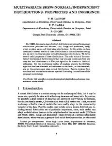
Figure captions Figure 1 Illustration of well positioning. The coordinate system is north, east and vertical depth. The position pk is estimated at each stand ( 30m) of the well path. The inclination is the angle between the vertical and the lateral coordinate. Azimuth is the angle between the two lateral coordinates. Figure 2 Data analysis of magnetic reference field observations at the geomagnetic observatory in Tromsø, Norway, in the year 2001. Magnetic declination (top), magnetic dip (middle) and magnetic strength (below). Left: Histogram with fitted normal (solid) and NIG (dashed) distribution. Middle: QQ plots using the normal distribution. Right: QQ plots using the NIG distribution. Figure 3 Well positioning distribution with NIG error source for magnetic declination angle. Diagonal entries represent marginals for north, east and vertical depth. Lower left displays are joint distributions for (north, east), (north, vertical) and (east, vertical). Upper right displays are well paths in north, east and vertical coordinates. Figure 4 Well anti-collision case 1. Diagonal entries show the marginals for offset well (blue) and reference well (black). Lower left displays show joint distributions for (north, east), (north, depth) and (east, depth) for both offset well (blue, circles) and reference well (black, crossed). Upper right displays show the well paths for offset well (blue) and reference well (black) in north, east and vertical depth coordinates. Figure 5 Well anti-collision case 1, when shifting the offset well on a grid of north, east coordinates. Top: p-values for the NIG model. Middle: p-value difference between NIG and normal case with Monte Carlo test. Below: p-value difference between NIG and normal case with approximate normal test. Figure 6 Well anti-collision case 2. Diagonal entries show the marginals for offset well (blue) and reference well (black). Lower left displays show joint distributions for (north, east), (north, depth) and (east, depth) for both offset well (blue, circles) and reference well (black, crossed). Upper right displays show the well paths for offset well (blue) and reference well (black) in north, east and vertical depth 24
coordinates. Figure 7 Well anti-collision case 2, when shifting the offset well on a grid of north, east coordinates. Top: p-values for the NIG model. Middle: p-value difference between NIG and normal case with Monte Carlo test. Below: p-value difference between NIG and normal case with approximate normal test.
25
Figure 1:
26
Density
100 80 60 40 20 0 −0.04
−0.03
−0.02
−0.01
0
0.01
0.02
0.03
0.04
Normal qq−plot 0.15
0.1
0.05
0
−0.05
−0.1 −0.1
Scaled magnetic declination (rad)
−0.05
0
0.05
0.1
0.15
Scaled magnetic declination (rad)
120
Scaled magnetic declination (rad)
140
200 150 100 50 0 −0.04
−0.02
−0.01
0
0.01
0.02
0.03
0.04
−0.1
−0.05
0.06 0.04 0.02 0 −0.02
0.04 0.02 0 −0.02 −0.04
−0.02
0
0.02
0.04
0.06
0.08
0.1
−0.04
−0.02
0
0.002 0 −2000
−1500
−1000
−500
0
500
1000
Scaled magnetic strength (nT)
1500
2000
2000 1000 0 −1000
−1000
0
1000
2000
Scaled magnetic strength (nT)
Figure 2:
27
0.04
0.06
0.08
0.1
NIG qq−plot
3000
−2000 −2000
0.02
Scaled magnetic dip (rad)
Scaled magnetic strength (nT)
Scaled magnetic strength (nT)
Density
0.004
0.15
0.06
Normal qq−plot
0.006
0.1
0.08
Scaled magnetic dip (rad)
0.008
0.05
0.1
Scaled magnetic dip (rad)
0.01
0
NIG qq−plot
0.08
−0.04
−0.1
Scaled magnetic declination (rad)
−0.04 −0.03
0
−0.05
Normal qq−plot Scaled magnetic dip (rad)
Scaled magnetic dip (rad)
Density
250
0.1
0.05
Scaled magnetic declination (rad)
0.1 300
NIG qq−plot 0.15
3000
3000 2000 1000 0 −1000 −2000 −2000
−1000
0
1000
2000
Scaled magnetic strength (nT)
3000
Figure 3:
28
Figure 4:
29
NIG p−values 100
0.001 0.001
0.01
0.01
50
0.00
0.1
1
0
1 0.0
North
0.25
−50
0.25
0.1
0.00
0.1
0.01
1
0.01 −60
−0.00
1
0 −100 −100
20
40
60
80
−0.004
.005 −0 −0.004
−0.003 −0 .0 04
−0.003
−0.002 004 −0. −0.005
−0.002
−0.001 −0.002
3
−0.001 −0.003
01
.0
−0
04
0 0.
−0.003 − −0.001
−0.002
0 East
20
0
0
0
−80
−60
100
.00
−0.003
0
−50
0 East
0
−0.002
50 0 North
−20
Difference in Monte Carlo normal and NIG p−values 0
0
100
−40
−0
−80
−0.005
−100 −100
0.001
−40
−20
40
60
80
100
80
100
Difference in approximate normal and NIG p−values 100
0
0
−0.1
−0.2 −0.3
−−00.6.5
−0
.1
−0
0
.4
−0.6
−0.3
North
50
1
−0.
−0.2
−50
0 −100 −100
−80
−60
−40
−20
0 East
Figure 5:
30
20
40
60
0
Figure 6:
31
NIG p−values 100
0.05
0.05
0.1
0.025 0.1
0.25
0.1
5
0.05
0.25
0
0.2
North
50
0.05
0.025
0.25
−50
0.05 −100 −100
0.1
0.25
0.1 −60
−40
0.025
0.05
0.1 −80
−20
0
20
40
60
80
100
East Difference in Monte Carlo normal and NIG p−values 100
−0.03 −0.03
−0.04
−0.06
4
−0.05 −40
0
−0.02
−0.03
−0.04
−20
−0.0
−0.05
−0.06
−0.04 −60
−80
6
5
.0
−0.01
−0.06
−0.03
3
−0.0
−0.03
−0.02
−0.03 −0.02 −0.05 −0.06
−0.0
5
−100 −100
−0.04
−0.05
0
−50
−0.0
−0.06
−0
North
−0.06
−0.02
−0.04 −0.05
−0.06
−0.04 −0.05
50
−0.03
−0.04 −0.05
−0.02
20
40
60
80
100
80
100
East Difference in approximate normal and NIG p−values 100 −0.1