Normal Modes of a Global Nonhydrostatic ... - AMS Journals

VOLUME 128

MONTHLY WEATHER REVIEW

OCTOBER 2000

Normal Modes of a Global Nonhydrostatic Atmospheric Model AKIRA KASAHARA

AND

JIAN-HUA QIAN*

National Center for Atmospheric Research,1 Boulder, Colorado (Manuscript received 11 June 1999, in final form 6 March 2000) ABSTRACT Anticipating use of a very high resolution global atmospheric model for numerical weather prediction in the future without a traditional hydrostatic assumption, this article describes a unified method to obtain the normal modes of a nonhydrostatic, compressible, and baroclinic global atmospheric model. A system of linearized equations is set up with respect to an atmosphere at rest. An eigenvalue–eigenfunction problem is formulated, consisting of horizontal and vertical structure equations with suitable boundary conditions. The wave frequency and the separation parameter, referred to as ‘‘equivalent height,’’ appear in both the horizontal and vertical equations. Hence, these two equations must be solved as a coupled problem. Numerical results are presented for an isothermal atmosphere. Since the solutions of the horizontal structure equation can only be obtained numerically, the coupled problem is solved by an iteration method. In the primitiveequation (hydrostatic) models, there are two kinds of normal modes: The first kind consists of eastward and westward propagating gravity–inertia oscillations, and the second kind consists of westward propagating rotational (Rossby–Haurwitz type) oscillations. In the nonhydrostatic model, there is an additional kind of eastward and westward propagating acoustic–inertia oscillations. The horizontal structures of the third kind are distinguished from those of the first kind by large differences in the equivalent height. The second kind is hardly affected by nonhydrostatic effects. In addition, there are so-called external inertia–gravity mode oscillations (Lamb waves), which propagate horizontally with almost constant speed of sound. Also, there are external rotational mode oscillations that correspond to equivalent barotropic planetary waves. Those two classes of oscillations are identical to those in the hydrostatic version of model. Nonhydrostatic effects on the first kind of oscillations become significant for smaller horizontal and deeper vertical scales of motion.

1. Introduction With the increased capability of electronic computers in both speed and memory, there is a trend to use higher horizontal and vertical resolutions in numerical weather prediction models. It seems difficult to successfully emulate subgrid-scale motions, those phenomena occurring in between the grid increments of numerical model, through the so-called physical parameterization that expresses the effects of subgrid-scale motions in terms of the variables of grid-scale motions. Paramount examples are such phenomena as the release of latent heat of water vapor in clouds and the interactions of clouds with solar and terrestrial radiations. It is more straightforward to use higher-resolution numerical models with appropriate

* Current affiliation: IRI/LDEO, Columbia University, Palisades, New York. + The National Center for Atmospheric Research is sponsored by the National Science Foundation. Corresponding author address: Dr. Akira Kasahara, National Center for Atmospheric Research, P.O. Box 3000, Boulder, CO 803073000. E-mail: [email protected]

q 2000 American Meteorological Society

explicit physics even though the spatial resolution of observation network is coarser than that of prediction models. Current numerical prediction models of global weather forecasts and climate simulation are based on a primitive-equation formulation (e.g., Kasahara 1996) with a hydrostatic assumption. Daley (1988) pointed out that nonhydrostatic effects become relevant for a global model that can resolve motions with a horizontal scale of two-dimensional wavenumber higher than 400, equivalent to the zonal wavelength of about 70 km in the midlatitudes. One distinction in nonhydrostatic model formulation is that sound waves can travel vertically as well as horizontally. Thus, in an explicit computational approach, a very small time step must be used to perform the time integration of model to allow the passage of acoustic waves between the consecutive grid points in the vertical. Semazzi et al. (1995) and Qian et al. (1998) developed a global nonhydrostatic model that can use the same time increment as used in primitive-equation models with comparable horizontal and vertical resolutions. Similar efforts have been made by Cullen et al. (1997). Marshall et al. (1997) and Smolarkiewicz et al. (1999) present numerical integration schemes for global nonhydrostatic incompressible ocean

3357

3358


and atmosphere models, respectively. However, acoustic modes of oscillations are filtered out in the latter models due to the modeling assumption of incompressibility. The objective of this article is to describe a unified approach to calculate the normal modes of a global nonhydrostatic, compressible, and baroclinic model. The normal modes are the characteristics of free small-amplitude oscillations of a dynamical system superimposed on a basic state (Lamb 1932). Here, we take an atmosphere at rest as the basic state for simplicity. Thus, the normal modes are obtained as the solutions of the equations of dynamical system without forcing linearized around the basic state of rest. Since the normal modes are exact solutions of the linearized equations, they are useful in many applications related to the solutions of nonlinear dynamical systems as basis functions, ranging from the time integration of the dynamical systems to the representations of model variables for objective analysis and data initialization. A general discussion on the normal mode of compressible, nonhydrostatic, and baroclinic atmosphere is found in, for example, a textbook by Gill (1982). Earlier, Monin and Obukhov (1959) presented the classification of normal modes of a nonhydrostatic atmosphere on a tangent plane. Eckart (1960) discussed on the normal modes of a general compressible, nonhydrostatic, baroclinic, and spherical atmosphere with various approximations. In particular, the normal modes with tangentplane approximations for an isothermal basic state are treated extensively. A recent discussion on Eckart’s theory using the WKB approximation is given by Phillips (1990). Dikii (1965) also investigated the characteristics of the normal modes of a spherical nonhydrostatic model. However, the case of spherical atmosphere has not been fully analyzed yet. Another recent reference is the work of Daley (1988), who has investigated this subject with applications to the time integration of a nonhydrostatic global model. In our present work, we adopted a different approach from Daley (1988) to obtain complete solutions. We present in section 2 the basic equations of a global nonhydrostatic model without forcing and diabatic effects. In section 3, a linearized set of the basic equations with respect to an atmosphere at rest is given. In section 4, we discuss how to separate the variables to form two sets of equations for the structures of normal modes in the horizontal and vertical directions. Here, our approach to the separation of variables differs from that of Daley (1988), who made the separation of variables in such a way that the frequency of normal modes appears only in the horizontal structure equation. Our approach is described in section 5. An eigenvalue–eigenfunction problem is set up, consisting of horizontal and vertical structure equations with respective boundary conditions. These equations contain the frequency of normal modes and a separation parameter that plays the role of ‘‘equivalent height’’ as the two unknowns to be determined. We say ‘‘separation parameter’’ instead of

VOLUME 128

the separation constant usually used in the normal-mode problem of the primitive equation model. In the primitive-equation problem too the linearized system is separated into the horizontal and vertical structure equations. In doing so, a parameter appears that connects the two equations and is identified as the equivalent height. Taylor (1936) demonstrated that the horizontal structure of normal modes and the associated frequency are identical to those of the oscillations of a shallow water model with the separation constant as its uniform depth. Then, the equivalent height is determined as the eigenvalue of the vertical structure equation. In the nonhydrostatic problem, the equivalent height no longer appears as the uniform depth of the shallow water model in the physical space, but it appears only in the modal space symbolically. Once this distinction in the role of separation parameter is understood, use of the term equivalent height is convenient in describing its relationship with the separation constant of the hydrostatic problem. From this point on, we treat the case of isothermal atmosphere, and the solutions of vertical structure equations are presented in section 6. Discussions on the determination of wave frequency and equivalent height are presented in section 7 for the hydrostatic model and in section 8 for the nonhydrostatic model. Results from the numerical solutions of frequency and equivalent height are discussed in section 9. Conclusions and further comments are presented in section 10. 2. Basic equations We express a nonhydrostatic global atmosphere in spherical coordinates with f as latitude, l as longitude, and z as the altitude relative to the earth’s radius a, which is treated as a constant. We adopt the ‘‘traditional approximations’’ (Phillips 1973) that lead to the so-called primitive equations, except that the hydrostatic approximation is not assumed. Thus, the surface of constant apparent gravitational potential is approximated by a sphere and the thickness of the atmosphere is assumed to be very small compared to the earth’s radius. Moreover, the earth’s gravitational acceleration, g, is assumed to be constant. By incorporating the above simplifications and other minor assumptions, the equations of motion, mass continuity, and thermodynamics for adiabatic motion together with the equation of state are written in the form (e.g., Gill 1982)

1 f 1 a 2y 5 2 ra cosf ]l , dy u tanf 1 ]p 1 1f 1 u52 , dt a 2 r a ]f du 2 dt

u tanf

dH

1

]p

dw 1 ]p 5 2g 2 , dt r ]z

(2.1)

(2.2) (2.3)

OCTOBER 2000

3359

KASAHARA AND QIAN TABLE 1. Definition of variables and symbols.

f l z t dH 5 1 dH 5 0 (u, y , w) p r T R Cp Cy 5 C p 2 R g k 5 R/Cp 5 (g 2 1)/g g a V

Latitude Longitude; also used as the eigenvalue of (6.4) Altitude Time For nonhydrostatic case For hydrostatic case Zonal, meridional, and vertical wind components Pressure Density Temperature Gas constant for dry air (5287.04 J Kg21 K 21 ) Specific heat at constant pressure (51004.6 J Kg21 K 21 ) Specific heat at constant volume 5 Cp /Cy (52/7) Earth’s gravitational acceleration (59.8 m s22 ) Earth’s radius (52 3 10 7 /p in m) Earth’s rotation rate [5p /(12 3 60 3 60) s21 ]

1

2

dr ]w 1 r =·V 1 5 0, dt ]z

(2.4)

dp dr 5 gRT , dt dt

(2.5)

p 5 rRT,

(2.6)

where d ] ] 5 1 V·= 1 w , dt ]t ]z

(2.7)

V·= 5

u ] y ] 1 , a cosf ]l a ]f

(2.8)

=·V5

1 ]u ] 1 (y cosf) , a cosf ]l ]f

V 5 (u, y ),

[

]

and

f 5 2V sinf.

(2.9) (2.10) (2.11)

The definitions of the variables and symbols are given in Table 1. One comment should be added here concerning our selection of the basic equations in the framework of traditional approximations. When the equations of motion are derived in the coordinate system, which is rotating, there appear the additional Coriolis terms ˆfw on the left-hand side of Eq. (2.1) and 2 ˆfu in Eq. (2.3), where ˆf 5 2V cosf, as well as the apparent acceleration terms uw/a 2 (uy /a) tanf in Eq. (2.1), y w/a 1 (u 2 /a) tanf in Eq. (2.2), and 2(u 2 1 y 2 )/a in Eq. (2.3), which are caused by the curvature of the coordinate surfaces. The omission of the apparent acceleration terms due to the curvature of coordinate surface may be justified by scale analysis for atmospheric motions. Although the effect of the Coriolis term 2fû in Eq. (2.3) is probably small and can be neglected (Phillips 1990), the exact nature of this additional Coriolis effect as a contribution to nonhydrostatic dynamics still remains to be fully explored, as noted by Eckart (1960). If the term 2fû is

kept in Eq. (2.3), then the term ˆfw must be retained in Eq. (2.1) to satisfy energy balance, even though it is small compared with the term 2 fy . 3. Linearized equations We consider the motions of small amplitude superimposed on the basic state defined by p0 5 p0 (z), and u 0 5 y 0 5 w0 5 0,

r0 5 r0 (z), (3.1) which satisfy the hydrostatic equilibrium dp0 5 2r0 g. (3.2) dz Here the subscript zero of a variable denotes the basicstate quantity. Introducing the superscript prime for a perturbation quantity, we write u 5 u9, y 5 y 9, w 5 w9, p 5 p0 (z) 1 p9, (3.3) r 5 r0 (z) 1 r9, T 5 T0 (z) 1 T9, where all perturbations are functions of l, f, z, and t. Substituting (3.3) into (2.1)–(2.5) and neglecting quantities of second and higher order, we obtain the following system of linear equations: ]u9 1 ]p9 r0 1 2 f r0 y 9 5 0, (3.4) ]t a cosf ]l ]y 9 1 ]p9 1 1 f r0 u9 5 0, ]t a ]f

(3.5)

]w9 ]p9 1 1 r9g 5 0, ]t ]z

(3.6)

]r 9 1 ]p9 r N2 2 2 2 0 w9 5 0, ]t Cs ]t g

(3.7)

r0

dH r0

1

2

1 ]p9 ]w9 2 r0 gw9 1 = · V9 1 5 0. 2 r0 Cs ]t ]z

(3.8)

3360


The derivation of these equations is standard. For example, Eqs. (3.7) and (3.8) correspond to (6.14.3) and (6.14.6), respectively, of Gill (1982). The parameter N 2 in (3.7) is defined by

1

2

1 dr0 g N 5 2g 1 2 , r0 dz Cs 2

and N has the dimension of frequency, referred to as the Brunt–Vaïsa¨la¨ frequency. Also, C 2s in (3.7) to (3.9) is defined by C 2s 5 g RT0 ,

(3.10)

and C s is referred to as the speed of sound in the basic state. 4. Separation of variables

r01/2 u9 ) ) U(f)j (z) ) r01/2 y 9 iV(f)j (z) 21/2 )r0 p9) 5 ) P(f)j (z) ) exp[i(sl 2 s t)], r01/2 w9 iP(f)h (z) 21/2 )r0 r9) ) P(f)z (z) )

) )

) ) ) )

) )

(4.1)

where s and s denote, respectively, the zonal wavenumber and the frequency. In the appendix we show that the frequency s of this system is real. By substituting (4.1) into (3.4)–(3.8), we get sP 5 0, a cosf

(4.2)

dP 5 0, adf

(4.3)

dj 1 dr 0 1 j 1 gz 5 0, dz 2r0 dz

(4.4)

N2 s h 2 2 j 5 0, g Cs

(4.5)

2sU 2 f V 1

f U 1 sV 1

dH sh 1

sz 1

[

1

[

]

1 d sU 1 (V cosf) 5 sHL (P), a cosf df

(4.7)

(4.8)

(4.9)

where HL [

[

s s a cosf (s 2

]

1 2 ss d 1 2V sinf . 1 2 f ) a cosf adf2

21 d 1 2V sinf d s 1 s cosf s a cosf df (s 2 2 f 2 ) a adf 2

(4.10) Here, H L ( · ) is known as Laplace tidal operator (cf. Longuet-Higgins 1968). As noted earlier, Eqs. (4.4)–(4.6) contain vertical functions, except for the horizontal divergence term in (4.6). Now, the horizontal divergence term is expressed as a function of P as seen from (4.9). Thus, the dependence on the horizontal function P in Eq. (4.6) can be eliminated by introducing the parameter of separation h e defined by HL (P) 5

1 P. gh e

(4.11)

Actually, this relationship used to separate Eqs. (4.2)– (4.6) into the horizontal and vertical systems of equations was first introduced by Taylor (1936) for a hydrostatic atmosphere and this procedure later became a tradition of tidal theory (e.g., Chapman and Lindzen 1970). Dikii (1965) has shown that the same procedure can be adopted to separate the system into the horizontal and vertical equations in the nonhydrostatic atmosphere too. By using (4.9)–(4.11), we can rewrite (4.6) compactly as

1C

2 s

]

2

2

1

s 1 d dh 2 2j 1 sU 1 (V cosf) jP 21 1 Cs a cosf df dz 1 dr0 g 2 1 2 h 5 0. 2r0 dz Cs

1 ss dP P 1 2V sinf , 2 (s 2 f ) a cosf adf 2

Calculation of the horizontal divergence term in (4.6) by using (4.7) and (4.8) yields

1

Since the coefficients of the derivatives of perturbation variables with respect to time, t, and longitude, l, are constant, we can express the perturbation variables in the form )

1 2 21 2V sinf dP V5 sP 1 s . (s 2 f ) 1 a cosf adf2

U5

2

(3.9)

VOLUME 128

2

2

1 sj 5 L 1 (h), gh e

(4.12)

where (4.6)

Equations (4.2) and (4.3) contain only meridional functions and no vertical functions. The remaining three equations, (4.4)–(4.6), contain vertical functions, except for the horizontal divergence term in (4.6). By rewriting (4.2) and (4.3), we have

L 1 (·) 5 G5

d(·) 2G dz

and

(4.13)

1

2

1 dr 0 g 1 g N2 1 25 2 , 2r0 dz Cs 2 Cs2 g

(4.14)

using (3.9). The quantity G plays a prominent role in the theory of atmospheric oscillations. Here, we use the same symbol as adopted by Eckart (1960) and Gill

OCTOBER 2000

(1982). It is important to note that the form of the vertical structure equation (4.12) does not depend explicitly on the choice of horizontal coordinates used which is implicit in the definition of h e given by (4.11). We will come back to discuss the significance of h e later. Next, we eliminate z between (4.4) and (4.5) and get (N 2 2 dH s 2 ) h 5 sL 2 (j ),

(4.15)

where L 2 (·) 5

d(·) 1 G. dz

(4.16)

By eliminating j between (4.12) and (4.15), we get L2

3361

KASAHARA AND QIAN

[1

21

2

1 1 2 Cs2 gh e

]

L 1 (h) 5 (N 2 2 dH s 2 )h.

(4.17)

This is the vertical structure equation governing the dependency of the density-weighted vertical velocity r1/2 0 w9 on the vertical coordinate z. 5. Eigenvalue–eigenfunction problems The linear system of Eqs. (4.2)–(4.6) with appropriate boundary conditions leads to a coupled eigenvalue–eigenfunction problem with the horizontal and vertical structure equations, respectively, in which the frequency s and the equivalent height h e appear in common. Let us first consider the eigenvalue–eigenfunction problem with the horizontal structure equation (4.11). The meridional eigenfunction P(f ) and the eigenvalue s that appears in the operator H L ( · ) defined by (4.10) can be solved with the lateral boundary conditions P50

at f 5

p p and 2 , 2 2

(5.1)

if the parameter h e is specified. In the context of global shallow water theory from which Eq. (4.11) is derived, h e signifies the depth of water in the basic state at rest. In fact, the eigenvalue–eigenfunction problem of (4.11) with (5.1) of the linearized nonhydrostatic system is identical to the same problem of linearized shallow water equation system in which the frequency s is determined uniquely for a given value of h e . As discussed in detail by Longuet-Higgins (1968), there are two kinds of eigensolutions. One is referred to as the oscillations of the first kind, which consist of eastward and westward propagating inertia–gravity waves. The other is the oscillations of the second kind, which are westward propagating planetary (Rossby–Haurwitz type) waves (Rossby et al. 1939). A method of solution is discussed by Kasahara (1976) and a computer code to calculate the frequency and structure functions for a positive value of h e is described by Swarztrauber and Kasahara (1985). Next, we consider the vertical part of the normalmode problem. The vertical structure function h(z) as defined in (4.1) can be determined from the vertical structure equation (4.17) with appropriate boundary

conditions in z. As the lower boundary condition, it is customary to assume that w9 5 0 at z 5 0. As the upper boundary condition, we generally require that the perturbation kinetic energy 12 r0 (u9 2 1 y 9 2 ) remain bounded as z → ` (Dikii 1965). In forced problems, such as atmospheric tides and lee waves, which deal with vertical wave propagation, a radiation condition is often assumed. In our case, we are considering the application of the normal modes to a numerical prediction model as the basis functions to represent the model variables as done in the case of the primitive-equation model (Kasahara and Puri 1981). Since prediction models require that the total mass be conserved in the system, we also assume that the upper boundary is rigid, that is, w9 5 0 at z 5 z T , the model top. Hence, the boundary conditions of (4.17) are chosen to be

h 5 0 at z 5 0 and z T .

(5.2)

The use of the rigid boundary conditions (5.2) is known to produce the internal modes of oscillations, which do not necessarily reflect the reality of the atmosphere (Lindzen et al. 1968). Nevertheless, it has been demonstrated that the vertical representation of model variables in terms of the vertical structure functions of internal modes is useful to atmospheric data analysis, particularly its application to nonlinear normal-mode initialization (Daley 1991). Once s, h e , P(f ), and h(z) are determined for a given value of the wavenumber s, the velocity component functions U(f ) and V(f ) are calculated from (4.7) and (4.8). The vertical structure functions j(z) and z(z) in (4.1) are calculated from (4.12) and (4.5). 6. Isothermal atmospheric case From this point on we treat the case of isothermal basic state, T0 5 const. This simplification leads to the parameters (3.9) and (3.10), which are now expressed by N2 5

kg , H

(6.1)

Cs2 5

gH , 12k

(6.2)

RT0 g

(6.3)

where H5

denotes the scale height. Here, all these quantities are constant. We introduced a new symbol, k, which is equal to R/C p . See Table 1. The vertical structure equation (4.17) can now be reduced to the form d 2h 1 (l 2 G 2 )h 5 0, dz 2 where l is expressed by

(6.4)

3362


1

2

1 1 2 2 (N 2 2 dH s 2 ) gh e Cs

l5

(6.5)

and the parameter G, as defined by (4.14), in the isothermal case is expressed as 1 2 2k 3 5 H 21 2H 14

G5

h(z) 5 A k sinkˆ z,

There is an additional solution to the system (4.2)– (4.6) in the case of isothermal atmosphere. A feature of this particular solution is that w9 in (3.6)–(3.8) or h(z) in (4.4)–(4.6) vanishes, namely, no vertical motions. In this case, as seen from (4.12), the equivalent height h e must be identical to a constant value as defined by

(6.6)

by using k 5 2/7; this is also shown on p. 172 of Gill (1982). The eigenfunction of (6.4) with the boundary conditions (5.2) can be written as (6.7)

h ex 5

kp . zT

(6.8)

Here, k is an integer 1, 2, . . . as the index of vertical mode. Substitution of (6.7) into (6.4) determines the eigenvalue l in the form

l k 5 kˆ 2 1 G 2

(6.9)

for the vertical index k 5 1, 2, . . . and the subscript k is added to l. The vertical structure function j(z) of the scaled velocity components and pressure is obtained by substituting (6.7) into (4.12) and we get

j (z) 5

1

2

1 1 2 2 Cs gh e

21

Ak [kˆ cos(kˆ z) 2 G sin(kˆ z)]. s

(6.10)

Thus, the coefficient A k can be determined from (6.10) in terms of the surface value j(0) and we get

1C

1

A k 5 j (0)

2 s

2

2

1 s kˆ 21. gh e

j(z) 5 j(0) exp(2Gz).

1C

1 2 s

2

2

1 s kˆ 21 sin(kˆ z). gh e

(6.15)

7. Determination of equivalent height and frequency (I): Hydrostatic model In the hydrostatic model, d H 5 0, (6.5) is simplified as

(6.12)

The vertical structure function z(z) of the scaled density can be calculated from (4.5) as 1 N2 z (z) 5 2 j (z) 2 h (z). Cs gs

(6.14)

Since the vertical motion in this case is identically zero, this particular mode of oscillations also appear in the hydrostatic model, d H 5 0. The oscillations are horizontally propagating waves consisting of the first and second kinds as discussed in section 5. The first kind of oscillations, consisting of westward and eastward propagating inertia–gravity waves, are referred to as Lamb waves (Eckart 1960; Gill 1982) after Lamb (1932, p. 548) who investigated wave propagation in a compressible isothermal atmosphere without rotation and found this special type of oscillation. In the case of global atmosphere with rotation, the second kind of oscillation are also present. Therefore, we will refer to this particular mode as the external mode instead of Lamb mode in contrast to the internal mode solutions presented earlier.

(6.11)

The surface value j(0) can be determined from a known distribution of the surface value of r21/2 p9 by using the 0 method of Hough harmonic expansion described in Kasahara (1978). Hence we have

h (z) 5 j (0)

Cs2 H 7 5 5 H. g 12k 5

For the earth’s atmosphere, the value of hex is approximately 10 km. The vertical structure function, j(z), must satisfy (4.15) with h(z) 5 0. Hence, we get

where kˆ is defined by kˆ 5

VOLUME 128

(6.13)

Note that the vertical structure functions j(z), h(z), and z(z) are functions of the vertical index k. As it will become clear later, both s and h e depend not only on k, but also on the wavenumber s and a meridional modal index yet to be defined. Since j(z), h(z), and z(z) include both s and h e , the vertical structure functions depend on the three-dimensional indices, k, s, and meridional index.

l5

1gh

1 ed

2

2

1 N2, Cs2

(7.1)

where hed denotes the equivalent height in the hydrostatic model. Since l is given by (6.9), the value of hed can be determined from (7.1) for each vertical index k 5 1, 2, . . . , in the form h ed 5 5

1

4k H 1 1 4kˆ 2 H 2

21

2

Cs2 C 2l 1 1 s 2k g N

(7.2a) (7.2b)

using the definitions of C 2s , N 2 , and G. Table 2 shows the values of hed , as a function of vertical index k calculated using the values of the constants given in Table 1 and assuming the isothermal atmosphere with T0 5 243.878 K and the model top of z T 5 18 km. Actually the value of T0 is selected in such a way that the external mode hex becomes equal to 10

OCTOBER 2000

3363

KASAHARA AND QIAN

TABLE 2. Values of the equivalent height hed in the hydrostatic case with To 5 243.878 K and zT 5 18 000 m. Note: l 5 0 denotes the external mode. Internal modes are represented by k 5 1, 2, . . . . The k 5 0 mode represents the internal mode in the case of infinite top, zT 5 `. Vertical mode k

hed in m

(l 5 0) 0 1 2 3 4 5 6

10 000.00 8163.26 1131.17 315.59 143.34 81.25 52.19 36.31

8. Determination of equivalent height and frequency (II): Nonhydrostatic model a. Coupled eigenvalue problem Although d H is equal to unity in the nonhydrostatic model, it is useful to keep symbol d H to investigate the modification of normal modes due to variation in the value of d H other than unity. For example, the ‘‘approximate’’ atmospheric model of Browning and Kreiss (1986) adopts the value of d H greater than unity in order to slow down the speed of high-frequency waves. Let us rewrite (6.5) and get

dH s 2 5 N 2 2 km. Butler and Small (1963) calculated the equivalent height of 10 km for free oscillations. Lindzen and Blake (1972) found that free oscillations in an unbounded atmosphere with a realistic earth temperature distribution are present for the equivalent height of 10 km. Since hed of the internal modes depends on the height of the model top assumed, hed forms a continuous spectrum in an unbounded atmosphere. However, once a finite model top is selected, hed forms a discrete spectrum. The internal modes of the discrete spectrum are denoted by the vertical mode index k 5 1, 2, . . . . However, there is a special solution corresponding to kˆ 5 0. By looking at (6.7), it appears as though h(z) vanishes. This is not the case here. From the expression of (6.12), at the limit of kˆ → 0, h(z) gives (G. Platzman 1999, personal communication)

1C

h (z) 5 j (0)

1 2 s

2

2

1 s z; gh e

(7.3)

namely, the variable r1/2 0 w9 varies linearly with height z. For a nonzero value of vertical mode index k, the vertical wavenumber kˆ tends to be zero as the model top z T approaches infinity; see Eq. (6.8). Thus, kˆ 5 0 corresponds to the limiting case of internal modes in the infinite atmosphere. By defining l0 for the value of l k in (6.9) in the case of kˆ 5 0, we have

l 0 5 G 2.

(7.4)

Also, from (7.2b) we get C2 40 h ed (kˆ 5 0) 5 4kH 5 4k (1 2 k) s 5 h ex . g 49

Cs2 gh e l k , (Cs2 2 gh e )

where l k is expressed by (6.9). Note that, since d H appears only in front of s 2 , the frequency s varies inversely proportional to the square root of d H . The parameter d H plays an analogous role of the aspect ratio (height/width) a discussed in Table 8.1 of Gill (1982). When a is small, the motions tend to be hydrostatic and become fully nonhydrostatic when a becomes close to unity. However, the parameter d H is directly tied to the wave frequency so that s 2 becomes smaller inversely proportional to d H when the value of d H is chosen greater than unity. The frequency s is also determined as the eigenvalue of Laplace tidal equation (4.11) with boundary conditions (5.1) for a given value of h e and zonal wavenumber s. The frequency s has a discrete spectrum with respect to meridional index ,, but we suppress explicit writing of the dependence of function on the meridional index unless it is necessary to do so. Thus, the frequency of s may be symbolically written as

s 5 F(h e , s).

This value is listed in Table 2 for k 5 0, and it is the largest value of hed in the internal modes of the hydrostatic model in the isothermal atmosphere. In the hydrostatic case, we can identify different vertical modes by using hed . The frequency s can then be determined from the horizontal structure equation (4.11) with the boundary conditions (5.1) for both the external and internal modes. However, this is not the case for the nonhydrostatic model, because the eigenvalue l of (6.5) contains both s and h e .

(8.2)

The characteristics of frequency equation (8.2) have been discussed already in section 5. Our task is to solve for s and h e simultaneously from (8.1) and (8.2). Although h e is no longer a constant parameter to characterize the normal modes of nonhydrostatic model, the parameter h e is still useful for identifying the different regimes of normal modes (Phillips 1990). In the range of h e that satisfies C 2s . gh e ,

(7.5)

(8.1)

(8.3)

we find from (8.1) that

dH s 2 , N 2 .

(8.4)

This means that in this range of h e , the nonhydrostatic frequency, s, becomes less than the frequency of Brunt– Vaïsa¨la¨ oscillation. On the other hand, if the range of h e satisfies C 2s , gh e ,

(8.5)

dH s 2 . N 2 ,

(8.6)

we find that

3364


contrary to (8.4). As seen from (6.14), the equivalent height of the external mode is given by C 2s /g. The significance in the presence of these two regimes of frequency will become clear from the asymptotic analysis presented in the next section. b. Approximate values of frequency and equivalent height Although the relationship between s and h e in (8.2) is transcendental, the solutions of coupled equations of (8.2) and (8.1) for s and h e can be obtained by an iteration method, starting from good initial guesses for the solutions. Although there is no easy way to obtain the analytical expression of (8.2), for a large value of h e it can be approximated by

s2 1

2Vs n(n 1 1) s2 gh e 5 0, n(n 1 1) a2

(8.7)

as given by Longuet-Higgins (1968). Here, s is the zonal wavenumber and n is the order of associated Legendre function P sn (cosf ) and n $ s. The integer n plays the role of meridional index. For the first meridional mode, it starts from n 5 s. Then the second mode corresponds to n 5 s 1 1, and so on. The solutions of quadratic equation (8.7) for s give approximate frequencies of the first kind oscillations, gravity–inertia waves. At the same level of approximation as one derives (8.7), an approximate s for the second kind oscillations is given by

s52

2Vs . n(n 1 1)

(8.8)

This solution is also discussed by Longuet-Higgins (1968), but earlier Haurwitz (1940) derived (8.8) by solving a linearized nondivergent vorticity equation over a sphere. Actually, Hough (1898) gave a higher approximate solution for this kind of oscillation than (8.8), and Haurwitz (1937) and Dikii and Golitsyn (1968) referred to it. Although we have not tested the utility of the higher approximate solution of this kind as the initial guess solution, we find that the formula (8.8) is not particularly useful for providing a good initial guess for the coupled eigenvalue problem. For the solutions of the second kind oscillations in the nonhydrostatic problem, those obtained from the corresponding hydrostatic model provides very good first-guess solutions for the iteration. This can be seen as follows. By rewriting (8.1), the functional dependence of h e on s can be expressed by he 5

1

2

C C lk 11 2 g N 2 dH s 2 2 s

2 s

21

.

(8.9)

Since the frequencies of the second kind oscillations are much smaller than N, the equivalent height h e given by (8.9) can be approximated accurately by the hydrostatic

VOLUME 128

value hed given by (7.2a). However, this is not the case for the first kind oscillations. By eliminating h e between (8.7) and (8.9), we obtain the following quartic equation:

dH s 4 1 dH As 3 2 (l k Cs2 1 N 2 1 dH B) s 2 2 A(l k Cs2 1 N 2 ) s 1 BN 2 5 0,

(8.10)

where A5

2Vs n(n 1 1) 2 and B 5 Cs . n(n 1 1) a2

(8.11)

There are four real solutions of (8.10) as two pairs of positive and negative frequencies. Once the frequencies are obtained, the corresponding equivalent height values can be calculated from (8.9). One pair corresponds to eastward and westward propagating very high frequency oscillations whose frequencies fall in the regime of (8.6) and the corresponding equivalent heights satisfy (8.5). This pair represents the acoustic–inertia mode, which appears uniquely in the nonhydrostatic model. The corresponding h e values are very large too. The other pair corresponds to eastward and westward propagating high-frequency oscillations whose frequencies fall in the regime of (8.4) with the corresponding equivalent heights, satisfying (8.3). This pair represents the gravity–inertia modes similar to that in the hydrostatic model. However, the similarity of the first kind oscillations in the nonhydrostatic model with those in the hydrostatic model applies only to planetary to largescale motions, as we will show later. c. Iteration method Our task now is to solve the simultaneous equations (8.2) and (8.1) by an iteration method using equivalent height h e as the iteration parameter. This means that starting from an initial guess of h e we vary the value of h e until the values of s from both equations (8.2) and (8.1) agree within a specified error tolerance. To do so, we must first investigate how s varies on h e in these equations. For a specific value of zonal wavenumber s in frequency equation (8.2), we know that the magnitude of s increases as h e increases. This can be verified numerically by solving Laplace tidal equation for s as a function of h e as shown in Figs. 2–6 of Longuet-Higgins (1968). To find out how s changes as h e varies in frequency equation (8.1), we differentiate it with respect to h e and obtain d(dH s 2 ) gC 4l 5 2 2 s k 2. dh e (Cs 2 gh e )

(8.12)

Since l k is always positive, (8.12) shows that the magnitude of s in (8.1) decreases as h e increases. Figure 1 shows schematically how the magnitude of s from the Hough frequency equation (8.2) and the

OCTOBER 2000

KASAHARA AND QIAN

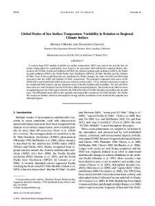
FIG. 1. Schematic diagram showing how the magnitude of frequencies calculated from Hough frequency equation (8.2) and nonhydrostatic frequency equation (8.1) vary as functions of equivalent height h e .

nonhydrostatic frequency equation (8.1) changes as the value of h e varies. Since the slopes of the two curves are opposite, we should be able to find the intersection of two curves that gives the unique solutions of s and h e that satisfy the two equations. All we need to have is a good initial guess hei and the information through (8.1) and (8.2) on how we should vary the increment Dh e for iteration in search of the solutions. It is important to note that the ordinate of Fig. 1 denotes the magnitude of frequency s instead of the value of s, which can be positive or negative depending on the type of solution. Therefore, the same search procedure applies to both eastward and westward propagating waves. Let us pick a value of h e denoted by the dotted line in Fig. 1. Then we calculate two s values, say s h , from the Hough frequency equation (8.2), and say s n , from the nonhydrostatic frequency equation (8.1) for a particular mode of solutions corresponding to given values of zonal wavenumber s, vertical mode index k, and meridional mode index. Next, we calculate another pair of frequencies, s h and s n , for the same particular mode by varying the value of equivalent height to h e 1 Dh e , where Dh e is a small positive value as a fraction of h e . If the magnitude of difference between |s h | and |s n | of the latter calculation is smaller than that of the former calculation, then the initial guess of h e is indeed located on the left-hand side of the linecrossing shown on Fig. 1. Therefore, the selection of h e 1 Dh e is an improvement over the initial guess of h e toward the desired solution. One can repeat this process successively to improve the accuracy of trial solution. The improvement of solution can be monitored through the reduction of the difference between |s h | and |s n |. However, this successive approximation process eventually leads to the situation in which the value of |s h | becomes larger than |s n |, corresponding to overshooting of the trial solution beyond the desired solution. Namely, this is the situation where the specification of h e goes on the right-hand side of the line crossing shown in Fig.

3365

1. Once this situation occurs, we know exactly where the desired solution is located by applying a suitable interpolation. Actually, linear interpolation gives an accurate solution for a sufficiently small value of Dh e . The successive approximation process is tedious, but it is logical and the convergence of solution is guaranteed. The success of this successive approximation method, which is referred to as method A, depends on the selection of a good initial guess of h e and the suitable choice of Dh e , which can be positive or negative. The choice of Dh e is different depending upon a particular normal mode and is selected by experimentation. For the acoustic–inertia mode, two high-frequency solution of (8.10) provide very good approximate solutions for any zonal wavenumber s and vertical mode index k. The initial guess values of he can be obtained from (8.9) using the approximate s values. Then, the desired solutions of s and h e are obtained using method A. For the gravity–inertia mode, two low-frequency solutions of (8.10) provide good approximate s values for large zonal wavenumber s . 400. For smaller zonal wavenumbers, it may be better to use the gravity–inertia mode frequencies calculated from the corresponding hydrostatic model as initial guesses. Then the h e values can be calculated from (8.9) and the s values can be updated through Hough frequency equation (8.2). In fact, we can iterate back and forth between equivalent height equation (8.9) and Hough frequency equation (8.2) to get converged solutions. We refer to this iteration technique as method B. However, the use of hydrostatic initial guesses for method B becomes ineffective for zonal wavenumber s . 50 and the solutions of (8.10) are used instead. It turned out that method B begins to fail for s . 400. This is because the solutions of (8.10) are so good that method B starts to give an overshoot of solution, meaning that the successive iteration yields too large corrections of h e for convergence. In this situation we can use method A. However, the solutions of (8.10) are correct to four to five decimal places. Therefore, for our presentation of results we use the solutions of (8.10) for s . 400. For the rotational mode (the second kind) oscillations, hydrostatic initial guesses are very accurate. Nonhydrostatic corrections can be made by applying method B. However, for all practical purposes the hydrostatic solutions are sufficiently accurate. 9. Results a. Meridional index and mode parity In this section, we present the frequency and equivalent height obtained from two frequency equations, (8.2) and (8.1), as the function of wavenumber s in graphical form. The variation of the horizontal pattern of normal modes in the longitudinal direction is identified by wavenumber s, which is well understood. How-

3366


VOLUME 128

TABLE 3. Parity of normal modes expressed by the meridional index , for a different value of zonal wavenumber s. SY: symmetric type, AY: antisymmetric type, N: nonexistent. Mode , 0 1 2 3

Acoustic

Gravity

s50

s.0

s50

s.0

N AY SY AY

SY AY SY AY

N AY SY AY

SY AY SY AY

Rotational s50 N N N N

s.0 AY SY AY SY

ever, the identification of global normal-mode patterns in the meridional direction is somewhat complicated by the fact that there are three kinds of oscillations as well as the parity of meridional components that will be designated by meridional index. Note that the horizontal patterns of acoustic and gravity modes are distinguished by large differences in the values of equivalent height h e . The horizontal structures of gravity (first kind) and rotational (second kind) modes are expressed as the solutions of the Laplace tidal equation (4.11), which are well understood as discussed in section 5. Because the associated Legendre functions are used to solve the Laplace tidal equation, Longuet-Higgins (1968) adopted the parameter n 2 s 5 0, 1, 2 and so on as meridional index, where n denotes the order of associated Legendre functions. However, we will use here another convention also adopted by Longuet-Higgins (1968), Kasahara (1976, 1977), and Swarztrauber and Kasahara (1985) to simply count the meridional modes by an integer , starting from zero as the lowest meridional mode. Table 3 shows the parity of the first four meridional modes in terms of index ,. Here, symbol SY denotes the symmetric type in which perturbation pressure p9 and zonal velocity u9 are symmetric with respect to the equator and meridional velocity y 9 is antisymmetric. Symbol AY denotes the antisymmetric type, having antisymmetric pressure and zonal velocity and symmetric meridional velocity. Symbol N indicates nonexistence. No acoustic and gravity modes exist corresponding to the lowest meridional index , 5 0 for s 5 0. Similarly, oscillations corresponding to the s 5 0 rotational mode are not present. [The nonexistence of s 5 0 rotational mode components creates a numerical nuisance for solving the global shallow water equations using Hough harmonic expansion as noted by Kasahara (1977) and a remedy was proposed by Kasahara (1978) by creating s 5 0 rotational mode basis functions. The latest discussions on the normal modes of Laplace tidal equation for s 5 0 are found in Tanaka and Kasahara (1992).] Special names are attached to some of the lowest meridional modes in Table 3. The lowest meridional component (, 5 0) of rotational mode is antisymmetric and corresponds to mixed Rossby–gravity waves as referred to by Matsuno (1966), who analyzed the structure of this particular mode using the equatorial beta-plane approximation and found that the oscillation has the character of gravity wave in a lower zonal wavenumber

FIG. 2. Frequency diagram for eastward propagating waves of nonhydrostatic model with infinite top, z T 5 `. Groups of three curves, denoted by A and G, are for acoustic and gravity modes, respectively, for meridional index , 5 0, 9, and 19. The straight line, denoted by B, represents the Brunt–Vaïsa¨la¨ frequency that divides acoustic and gravity mode regimes. Three curves that are almost straight lines, denoted by E, represent external gravity modes corresponding to meridional index, , 5 0, 9, and 19 for equivalent height of 10 km.

regime, but for a higher zonal wavenumber it behaves like a rotational wave. Likewise, the lowest meridional component (, 5 0) of eastward propagating gravity mode is symmetric and corresponds to Kelvin wave (Matsuno 1966). Except for s 5 0 and the rotational modes, there are two types of oscillations, eastward and westward propagating waves. In the case of s 5 0 in the acoustic and gravity modes, there are two frequencies of same magnitude and opposite sign. We begin our discussion of results from the eastward propagating wave frequency. b. Eastward propagating wave frequency diagrams Figure 2 shows a frequency diagram for eastward propagating nonhydrostatic waves corresponding to the case of infinite atmospheric top, z T 5 ` or the vertical mode index k 5 0. The abscissa denotes wavenumber s and the ordinate is the dimensionless frequency n scaled by 2V. All the frequency values used in the figures and related discussions are dimensionless, while the unscaled frequency s is used in the text. The straight line, denoted as B at n 5 136.128, represents the Brunt– Vaïsa¨la¨ frequency. The groups of three curves, denoted by A and G, are for the acoustic and gravity modes, respectively, for meridional index, , 5 0, 9, and 19 corresponding to the first, 10th, and 20th meridional modes. Those three curves give some idea about how the acoustic and gravity frequency domains, denoted by

OCTOBER 2000

KASAHARA AND QIAN

FIG. 3. Same as Fig. 2, except that this is a blowup of the lowerleft quadrant of Fig. 2.

A and G, will be filled by higher meridional modes. The group of three curves that are almost straight lines, denoted by E, represents for the external gravity mode corresponding to three meridional indices, , 5 0, 9, and 19 for the equivalent height of 10 km in this model. As discussed in section 6, in an isothermal atmosphere the external mode oscillations appear in common in the hydrostatic and nonhydrostatic models, because the vertical velocity vanishes entirely. In terms of the phase speed of external mode waves, they travel with speed slightly larger than the speed of sound, C s 5 313.05 m s21 . In order to see more clearly the frequency curves in a low wavenumber regime, Fig. 3 shows a blowup of the lower-left quadrant of Fig. 2. We find that the gravity mode (G) frequency is less than the external gravity mode (E) frequency for the same pair of meridional index , and wavenumber s, except that the E mode and G mode frequencies of , 5 0 coincide at s 5 0. In contrast, as seen from Fig. 2, the acoustic mode (A) frequency is greater than the E mode frequency for the same pair of , and s, but the A mode frequency approaches the E mode frequency of the same , in a high wavenumber regime. It is instructive to show in Fig. 4 the eastward propagating frequency diagram for the hydrostatic model, with the same vertical mode index k 5 0, to compare with Fig. 2. The group of three curves denoted by H present the hydrostatic gravity mode frequencies for , 5 0, 9, and 19, which should be compared with the G modes in Fig. 2. In this case, all the frequencies are uniquely determined by the single value of the equivalent height given by (7.5). The three curves marked as

3367

FIG. 4. Same as Fig. 2, except that this is the hydrostatic case, d H 5 0. Three lines, denoted by H, represent hydrostatic gravity mode frequencies for , 5 0, 9, and 19. No acoustic mode appears in hydrostatic model.

E represent the external gravity mode frequencies for , 5 0, 9, and 19, which are identical to those shown in Figs. 2 and 3. In comparing Figs. 4 and 2, we notice that the G mode frequencies start to deviate from the hydrostatic gravity mode (H) frequencies around s 5 400 as noted also by Daley (1988). While the G mode frequencies approach the Brunt–Vaïsa¨la¨ frequency as s increases in the nonhydrostatic model, the hydrostatic counterparts are kept increasing with s. Moreover, the slopes of the H mode frequency curves are almost constant with slightly smaller slopes than the E modes. Thus, the H waves are nondispersive. Another unique aspect of the hydrostatic model is devoid of the acoustic mode. c. Westward propagating wave frequency diagrams Figure 5 shows the same as Fig. 2, except for the case of westward propagating wave frequency, where frequency values are negative. Although Fig. 5 looks like a mirror image of Fig. 2 with the change of sign, the magnitude of the westward wave frequency is larger than that of the eastward wave frequency for the same s and ,. In the case of gravity modes, the differences in the magnitudes of frequency are significant in lower values of s and , but the differences become very small in higher values of s and ,. Recall that the lowest (, 5 0) eastward gravity mode is the Kelvin wave whose magnitude of frequency is significantly smaller than that of the lowest (, 5 0) westward gravity mode. However, those differences are still small relative to the scale of frequency in Fig. 5. In the case of acoustic modes, the

3368


FIG. 5. Same as Fig. 2, except that this is for westward propagating waves so that frequencies are negative.

VOLUME 128

FIG. 6. Same as Fig. 4, except for westward propagating waves.

d. Equivalent-height diagrams eastward and westward differences in the magnitudes of frequency are practically indistinguishable in low wavenumbers, but they begin to show up very slightly in higher wavenumbers. Figure 6 shows the same as Fig. 4, except for the case of westward propagating wave frequency. All the frequencies in the hydrostatic model are associated with the equivalent height given by (7.5). Again by comparing Figs. 5 and 6, we see deviations of nonhydrostatic gravity wave frequencies from the hydrostatic counterparts in a higher wavenumber regime. One distinction in the eastward and westward propagating waves is that there are westward propagating rotational modes as the oscillations of the second kind. Figure 7 shows the magnitudes of rotational mode frequency for , 5 0, 9, and 19, corresponding to the case of infinite atmospheric top, equivalent to k 5 0. Note that the , 5 0 component is known as the mixed Rossby–gravity wave. These frequency values are virtually identical to the hydrostatic counterparts. The magnitudes of nonhydrostatic frequencies are slightly smaller than the hydrostatic counterparts by no more than 1.E27. Thus, the nonhydrostatic effects on the oscillations of the second kind are negligible. Note that, as we have been saying, the external mode oscillations appear in both the nonhydrostatic and hydrostatic models in common. This is true in the rotational modes too. The magnitudes of external rotational mode frequencies with the equivalent height of 10 km are slightly larger than those shown in Fig. 7. However, the differences are indistinguishable in Fig. 7.

The horizontal structures of acoustic and gravity modes are distinguished by large differences in the values of equivalent height. Thus, the information on equivalent height is very important in distinguishing the acoustic modes from the gravity modes. Figure 8 shows the equivalent heights as the function of s for eastward propagating waves in the case of k 5 0. Three curves

FIG. 7. Frequency diagram for (westward propagating) rotational waves of nonhydrostatic model with infinite top, z T 5 `. Three curves for , 5 0, 9, and 19 are shown.

OCTOBER 2000

KASAHARA AND QIAN

FIG. 8. Equivalent-height diagram for eastward propagating waves of nonhydrostatic model with infinite top, z T 5 `. Groups of three curves, denoted by A and G, are for acoustic and gravity modes, respectively, for meridional index , 5 0, 9, and 19. Straight line shows equivalent height of 10 km for the external mode that separates acoustic and gravity mode regimes.

indicated by A are for the acoustic modes, , 5 0, 9, and 19. Note that the values of h e are very large in low wavenumbers but decrease very quickly toward higher wavenumbers and asymptote to 10 km, which is the external mode equivalent height. Three curves indicated by G are for the gravity modes, , 5 0, 9, and 19. The h e values are close to the hydrostatic case of 8163.265 m, given by (7.5), at low wavenumbers and they decrease gradually toward higher wavenumbers. The corresponding h e diagram for the westward propagating waves looks exactly the same as Fig. 8 and is not shown here. However, the h e values for westward propagating acoustic and gravity modes are very slightly smaller than those of eastward propagating waves. For the westward propagating rotational waves, the h e values in the nonhydrostatic model are virtually identical to the hydrostatic value of 8163.265 m. Slight differences are found in low wavenumbers, where the smallest value of 8163.252 m is found at s 5 1 and , 5 0. e. Remarks on the normal modes of higher vertical modes So far, we presented the results of s and h e of the nonhydrostatic model with an infinite atmospheric top (k 5 0). In this section, we will discuss the normal modes of higher vertical modes. As an example of higher vertical modes, we choose the top of isothermal atmosphere to be at z T 5 18 km as done in the example

3369

FIG. 9. Same as Fig. 8, except for the vertical mode, k 5 2.

shown in Table 2. We also select the second vertical mode for presentation here. For this atmosphere, in the hydrostatic model the value of equivalent height becomes 315.59 m corresponding to k 5 2 in Table 2. Silva Dias and Bonatti (1985) show that large-scale tropical motions are characterized by an internal mode with an equivalent height on the order of 250 m. Figure 9 shows the h e diagram for the nonhydrostatic eastward propagating waves in the same way as in Fig. 8, except for the vertical mode k 5 2. Three curves that belong to group A are for the acoustic mode. We see that the h e values of acoustic mode are much larger than those shown in Fig. 8. Group marked G denotes for the gravity mode and actually consists of three curves for , 5 0, 9, and 19, but the values for different meridional modes are very close each other so that three curves look like only one. The h e values are close to the hydrostatic case of 315.59 m at low wavenumbers and decrease rather slowly toward higher wavenumbers. The straight line for h e 5 10 km for the external mode separates the acoustic and gravity mode regimes. The h e diagram for the westward propagating acoustic and gravity modes is very similar to Fig. 9 and is not shown here. Their magnitudes are slightly smaller than those of the eastward propagating acoustic and gravity modes, respectively. We have noted in section 9c that the magnitudes of westward propagating frequencies of both acoustic and gravity modes, respectively, are slightly larger than those of corresponding eastward propagating waves. For the rotational waves, the h e values of the nonhydrostatic model are virtually identical to the hydrostatic value of 315.59 m. Figure 10 shows the frequency diagram for westward

3370



propagating second vertical mode (k 5 2) for comparison with Fig. 5 in the case of k 5 0. Note an expanded scale of frequency in the ordinates. The external mode frequencies, E, and the Brunt–Vaïsa¨la¨ frequency, B, provide the references as in Fig. 5, to find where the frequencies of A and G modes for k 5 2 are positioned relative to those of k 5 0. Namely, while the acoustic wave frequency of a higher vertical mode increases as k increases, the gravity wave frequency of a higher vertical mode decreases as k increases. These characteristics correspond to the discussion related to the h e diagram shown in Fig. 9. We pointed out that the h e value of acoustic k 5 2 mode is much larger than that of acoustic k 5 0 mode for the same s and ,. By contrast, the h e value of gravity k 5 2 mode is much smaller than that of gravity k 5 0 mode for the same s and ,. Thus, we see that the acoustic and gravity mode frequencies are greatly affected by the vertical mode index k. To demonstrate how the hydrostatic assumption modifies the above consideration, we show in Fig. 11 the same situation as in Fig. 10, except in the case of the hydrostatic model. It is clear that the acoustic mode is completely missing, but the frequency of gravity mode for k 5 2 is relatively intact by the hydrostatic assumption. This implies that the hydrostatic assumption is effective for the motion of small aspect ratio (height/ width). With respect to the rotational wave frequencies, we find that the nonhydrostatic model produces virtually no change in comparison with the hydrostatic model. However, as shown in Fig. 12, the magnitude of rotational wave frequency for k 5 2 becomes slightly smaller than

VOLUME 128


that of k 5 0, which is almost identical to that of the external mode for the same s and ,. 10. Conclusions and further comments In this article, a unified approach is described to calculate the normal modes of a nonhydrostatic, compress-

FIG. 12. Same as Fig. 7, except for the vertical mode, k 5 2. In addition, external mode frequencies for , 5 0, 9, and 19 are plotted. Notice some differences between the frequencies of k 5 2 mode and external mode for the same meridional index near the frequency maxima.

OCTOBER 2000

3371

KASAHARA AND QIAN

ible, baroclinic, and rotating spherical atmosphere with respect to a basic state at rest. Numerical results are presented for an isothermal atmosphere. Emphasis is made to focus on the differences between the normal modes of nonhydrostatic model and those of the corresponding hydrostatic model that have been studied extensively in the past. In the hydrostatic model, there are two kinds of normal modes: One is called the first kind, which consists of eastward and westward propagating gravity–inertia (or simply gravity) oscillations. The other is called the second kind, which consists of westward propagating planetary (Rossby–Haurwitz type) oscillations or waves. In addition, there are horizontally propagating oscillations, consisting of the first and second kinds with no vertical velocity in an isothermal atmosphere. They are classified as the external modes, corresponding to the equivalent height of 10 km in an earthlike isothermal atmosphere. The first kind of oscillations, consisting of westward and eastward propagating gravity waves, are referred to as Lamb waves, which propagate with approximately the speed of sound. The second kind of oscillations, consisting of westward propagating rotational waves, have the same characteristics of equivalent barotropic planetary waves. Note that the external modes are discrete in the model atmosphere, while the internal modes form a continuous spectrum of frequency depending on the vertical scale of motion in an unbounded atmosphere. However, in a bounded atmosphere the internal modes also become discrete. In the nonhydrostatic model, sound waves propagate vertically as well as horizontally due to the acceleration term in the vertical equation of motion. These additional oscillations are referred to as the acoustic–inertia (or simply acoustic) modes. It may be appropriate to call them the oscillations of the third kind. Their frequencies are much larger than those of the first kind. In solving the nonhydrostatic normal mode problem, a coupled eigenvalue–eigenfunction problem is set up, consisting of horizontal and vertical structure equations with respective boundary conditions, both of which contain the frequency of normal modes and the separation parameter h e , which plays a similar role of equivalent height in the traditional hydrostatic normal mode problem. In the hydrostatic model, the eigenvalue of vertical structure equation contains only the separation parameter. Therefore, the vertical structure equation is first solved to determine the value of the separation parameter, which is interpreted as a uniform depth of the shallow water model. This eigenvalue is referred to as equivalent height. In the hydrostatic problem, the first and second kind of internal modes are uniquely determined by a spectrum of equivalent height h e , which depends only on the vertical mode index. In the nonhydrostatic normal mode problem, the equivalent height h e depends not only on the vertical mode index k, but also on the zonal wavenumber s and the meridional index ,. Therefore, the physical inter-

pretation of h e in the hydrostatic model is no longer applicable to the nonhydrostatic case. Nevertheless, the concept of equivalent height h e plays an important role in distinguishing the first and third kinds of normal modes in the nonhydrostatic model. The acoustic (third kind) modes are characterized by very large values of h e , satisfying the condition (8.5). By contrast, the gravity (first kind) modes are characterized by small values of h e , satisfying the condition (8.3). Since the first and third kinds of oscillations both satisfy the Laplace tidal equation with their specific values of h e , the fact that the first and third kinds of normal modes are associated with large differences in their values of h e has an important implication on the horizontal structure of normal modes. Because the values of h e are extremely large for the acoustic modes, their frequencies are well approximated by

s56

[

]

n(n 1 1) gh e a2

1/2

,

(10.1)

as seen from (8.7) by neglecting the effect of rotation. Thus, from the asymptotic analysis of Longuet-Higgins (1968), the eigenfunctions of acoustic modes are described very nearly by a single spherical harmonic for the velocity potential F F } P sn (cosf ) exp[i(sl 2 st)]

(10.2)

and the vanishing streamfunction C 5 0. Daley (1988) discussed these characteristics of acoustic modes from the standpoint of high-frequency approximation. Concerning the eigenfunctions of normal modes, our study focused on the frequency aspect of normal modes and not so much on the eigenfunction aspect of normal modes. The reason we did not discuss the eigenfunction aspect in this paper is as follows. While the second kind of normal modes is distinctly different from the first and third kinds (see section 9a), the eigenmodes of the first and third kinds share similar characteristics, such as the parity shown in Table 3, except that a large difference in the equivalent height values separates the two kinds of normal modes. Moreover, the horizontal structures of nonhydrostatic normal modes can be obtained from those of the linearized shallow water model for given values of h e (see section 5). Therefore, once the values of h e are obtained for given values of vertical mode index k, zonal wavenumber s, and meridional index ,, the computer code of Swarztrauber and Kasahara (1985) is applicable to calculate the eigenfunctions of the acoustic normal modes as well as the gravity modes. Longuet-Higgins (1968) presented in graphical form the meridional profiles of the eigenfunctions of the first and second kinds of global normal modes as the solutions of Laplace tidal equation for up to zonal wavenumber 2 and various values of the dimensionless parameter defined by

3372


e5

4V 2 a 2 gh e

(10.3)

in the range of e 5 1, 10, 10 2 , and 10 3 . These e values corresponds to h e 5 87 483, 8748, 875, and 87 in meters for the earth. Hence the case of e 5 1 corresponds to the value of h e representative to the acoustic modes, e 5 10 corresponds to the external modes and rotational modes, e 5 10 2 corresponds to the gravity modes, and e 5 10 3 corresponds to the higher vertical gravity modes. As seen from Figs. 7–13 of Longuet-Higgins (1968), the meridional profiles of the eigenfunctions appear in global extent for small e or large h e , while they tend to become equatorially trapped for large e or small h e . Thus, for a set of the three-dimensional modal indices (s, ,, k), the acoustic mode eigenfunctions cover between the poles more uniformly than the gravity mode eigenfunctions. In addition to the presence of acoustic modes, the gravity modes of the nonhydrostatic model are significantly different in both the frequency and the meridional structure from those of the hydrostatic model for smaller-scale motions with a large aspect ratio. In fact, as seen from Fig. 4, the infinite-top internal (k 5 0) gravity modes of the hydrostatic model are very similar to Lamb waves, having almost constant propagation speeds. Hence, they are nearly nondispersive. This is not the case of nonhydrostatic model. As seen from Fig. 2, the k 5 0 gravity mode frequencies never exceed the Brunt–Vaïsa¨la¨ frequency. Also, as seen from Fig. 8, because of the differences in h e between the hydrostatic and nonhydrostatic gravity modes, their meridional structures are different too. Thus, the behaviors of gravity waves in the two models can be quite different even for medium-scale motions in the atmosphere. However, as far as the second kind oscillations are concerned, nonhydrostatic effects are virtually insignificant on their frequencies and structures. Further comments are made concerning applications of the nonhydrostatic normal modes. Since normal modes are the exact solutions of a linearized dynamical system, the utility of normal modes for global primitiveequation models has been well demonstrated in many applications of numerical prediction modeling. For example, normal-mode initial conditions are used to locate coding errors in the dynamics part of global primitiveequation model (Chao and Geller 1982) and to compare the accuracy of various numerical approximations to the global shallow water equations (Williamson et al. 1992). Three-dimensional global atmospheric data can be analyzed spectrally in three indices (zonal wavenumber, and meridional and vertical modal indices) using the normal modes of a global primitive-equation model (Kasahara and Puri 1981; Tanaka et al. 1986). The threedimensional primitive-equation normal modes are used as the basis functions for discretizing the time-dependent primitive equations (Kasahara and Tanaka 1989; Baer and Zhang 1999). Of course, a celebrated appli-

VOLUME 128

cation of the three-dimensional normal modes to the practice of nonlinear normal-mode initialization for primitive-equation models is well known (Baer and Tribbia 1977; Machenhauer 1977). All research topics referred to so far as the applications of primitive-equation normal modes become equally relevant to the applications of nonhydrostatic global normal modes. Since the development of global nonhydrostatic prediction models has just begun, we anticipate that the research history of global primitiveequation normal modes for numerical weather prediction will be repeated in global nonhydrostatic modeling as well. For example, there is the need for formulating the discretized version of normal modes for specific nonhydrostatic prediction models, as has been done in the case of primitive-equation models (Dickinson and Williamson 1972; Errico and Eaton 1987). The present study based on the analysis of continuum dynamics can be used as a guide to formulating the discretized version of global nonhydrostatic normal modes for specific prediction models with special attention paid to handling of acoustic modes. Further comments are in order here concerning the nature of normal modes treated in this study. (i) When the basic equations (2.1)–(2.5) are linearized, we assumed an atmosphere at rest as the basic state without consideration of advection effects by the background flow. Not only for mesoscale motions, the advection effects are important even for large-scale motions. The problem, however, is that the inclusion of advection terms greatly increases the complexity of the normalmode problem in this case. Even without the advection terms, the global nonhydrostatic normal-mode problem has never been completely solved in spite of a long history of research on the free oscillations of the atmosphere. Now, since the basic approach has been established, this may open the possibility of investigating the problem with a higher level of model complexity. Clearly, the inclusion of advection effects is such a candidate for a future study. (ii) In our study, we similarly neglected the effect of orography. In order to take into account the orographic effects in the prediction model, it is convenient to write the basic equations using terrain-following transformed vertical coordinates. In the case of the hydrostatic model, the global normal modes of the sigma coordinate primitive equation model have been obtained, for example, see Kasahara and Puri (1981). Hence, a similar procedure would be applicable to the nonhydrostatic model as well. However, the use of normal mode may not give a ‘‘well-posed’’ representation of the model variables in a high-resolution nonhydrostatic model in the region where a strong flow occurs near high mountains. Of course, this difficulty is not inherent in the use of normal mode per se, but it originates from the nature of spectral representation related to the famous Gibbs phenomenon in Fourier series theory. Clearly, we need to apply a special topographic filter, but such research

OCTOBER 2000

3373

KASAHARA AND QIAN

falls outside of the present objective. (iii) By definition of normal modes, diabatic effects are not considered in this study. However, the effects of diabatic forcing in the nonhydrostatic global model can be investigated using the present normal modes. Sotack and Bannon (1999) discussed a prototype problem of hydrostatic adjustment, that is, how the hydrostatic equilibrium is established from a hydrostatically unbalanced state, resulting from time-dependent heating. Understanding of hydrostatic adjustment is a prerequisite to studying the problem of data initialization with the nonhydrostatic model just as in the case of geostrophic adjustment (e.g., Blumen 1972) in a primitive equation model. The use of normal mode expansion greatly simplifies the treatment of hydrostatic adjustment, as well as the geostrophic adjustment in any coordinate system including spherical geometry. As a final note, we should mention that we performed the analysis of nonhydrostatic normal modes in an isothermal atmosphere using midlatitude and equatorial beta planes. Lindzen (1967) pointed out that the normal modes of a rotating global shallow water model can be approximated well by using two beta planes: one centered at the equator and the other at a midlatitude. We find that use of these two beta planes can provide good approximations to describe the characteristics of nonhydrostatic global normal modes and helps to interpret the numerical results from analytical consideration. Detailed discussion on this topic will be the subject of a separate article by J.-H. Qian and A. Kasahara. Acknowledgments. We would like to thank Prof. Moody T. Chu of the North Carolina State University for his suggestions on this work. We would also like to express our appreciation to Prof. George W. Platzman, who kindly read an earlier version of the manuscript and offered us many constructive suggestions to improve the article. A partial support to the first author is provided through a research collaboration between NCAR and the Central Research Institute of Electric Power Industry, Japan. The second author thanks Dr. Filippo Giorgi for his support during the course of this work. The manuscript was typed by Barbara Ballard at NCAR. APPENDIX Orthogonality of Normal Modes We show here that the frequency of normal modes described by Eqs. (3.4)–(3.8) is real and the modes are

(n j 1 n k*)

E[ V

orthogonal, following the procedure used by Platzman (1972). For this purpose, we assume that the prognostic variables u9, y 9, w9, p9, and r9 are proportional to exp(n t) where n is a complex number. Also, we introduce the new variable u9 defined by

u9 5

g p9 2 gr9, Cs2

(A.1)

which will be used in place of r9. Thus, we obtain the following new set from (3.4) to (3.8) without using the superscript prime, but adding the subscript j to indicate the jth normal mode:

n j r0 u j 5 2

1 ]pj 1 f r0 y j , a cosf ]l

(A.2)

n j r0 y j 5 2

1 ]pj 2 f r0 u j , a ]f

(A.3)

]pj g 2 2 pj , ]z Cs

(A.4)

dHn j r0 wj 5 uj 2 nj u 5 2wj , r0 N 2 j

(A.5)

nj ]wj g p 5 2= · Vj 2 1 2 wj . 2 j r0 Cs ]z Cs

(A.6)

We now show that the n j is pure imaginary and the modes (u j , y j , w j , u j , p j ) are orthogonal. We multiply (A.2)–(A.6) of the jth mode by u*k , y *k , w*k , u*k , and p*k , respectively, where the asterisk denotes complex conjugate. Also, we create another set by multiplying the complex conjugate forms of (A.2)–(A.6) for the kth mode by u j , y j , w j , u j , and p j , respectively. We then add these two sets of equations and obtain

1

(n j 1 n k*) r0 u j u*k 1 r0 y j y *k 1 dH r0 wj w* k 1 5 2= · (Vj p*k 1 V*k pj ) 2

pj p*k ujuk* 1 r0 Cs2 r0 N 2

2

] (w p* 1 w*k pj ). ]z j k

By integrating the above equation over the volume, V, on the sphere with radius a that extends from the surface z 5 0 to z 5 z T , the top, and assuming that the vertical velocity vanishes at the bottom and top, we get the following equation after multiplying the result by ½:

]

pj p*k ujuk* r0 (u j u*k 1 y j y *k 1 dH wj w*) 1 1 dV 5 0, k 2 2 2r0 Cs 2r0 N 2

(A.7)

3374


where dV 5 a 2 cosf df dl dz. For a nontrivial solution, the integral of total energy, TE, over the volume V must be positive; namely, TE 5

E

(K 1 E 1 A) dV . 0,

(A.8)

1 K 5 r0 (|u j | 2 1 | y j | 2 1 dH |wj | 2 ), 2

(A.9)

V

where

E5

1 | pj | 2 , 2 r0 Cs2

(A.10)

A5

1 | uj | 2 . 2 r0 N 2

(A.11)

Therefore, we find that n j 1 n *j 5 0, which means that the real part of n j does not exist; consequently, n j is purely imaginary and n j 1 n *k does not vanish for j ± k. Hence, we have

E[ V

]

uju *k pj p*k r0 (u j u*k 1 y j y *k 1 dH wj w*) 1 1 dV k 2 2 2r0 Cs 2r0 N 2

50

for j ± k.

(A.12)

This is the orthogonality condition of the normal modes. Eckart (1960) presented this orthogonality condition without detail and proposed the method of normal mode expansion. Platzman (1992) presents insight on Eckart’s expansion theorem, as well as a history on the use of normal-mode expansion to solve geophysical problems. The quantity K of (A.9) is the kinetic energy. Eckart (1960) called the quantity E of (A.10) the elastic energy from acoustics and the quantity A of (A.11) the thermobaric energy. Quantity A, which is proportional to the square of entropy perturbation, has a connection to the available potential energy by Lorenz (1955). REFERENCES Baer, F., and J. J. Tribbia, 1977: On complete filtering of gravity modes through nonlinear initialization. Mon. Wea. Rev., 105, 1536–1539. , and B. Zhang, 1999: An efficient time integration scheme for climate prediction models. Tellus, 51A, 652–662. Blumen, W., 1972: Geostrophic adjustment. Rev. Geophys. Space Phys., 10, 485–528. Browning, G. L., and H.-O. Kreiss, 1986: Scaling and computation of smooth atmospheric motions. Tellus, 38A, 295–313. Butler, S. T., and K. A. Small, 1963: The excitation of atmospheric oscillations. Proc. Roy. Soc. London, A274, 91–121. Chao, W. C., and M. A. Geller, 1982: Utilization of normal mode initial conditions for detecting errors in the dynamical part of primitive equation global models. Mon. Wea. Rev., 110, 304– 306. Chapman, S., and R. S. Lindzen, 1970: Atmospheric Tides: Thermal and Gravitational. Gordon and Breach, 200 pp. Cullen, M. J. P., T. Davies, M. H. Mawson, J. A. James, S. C. Coulter, and A. Malcolm, 1997: An overview of numerical methods for

VOLUME 128

the next generation U.K. NWP and climate model. Numerical Methods in Atmospheric and Oceanic Modelling: The Andre J. Robert Memorial Volume, C. A. Lin et al., Eds., NRC Research Press, 425–444. Daley, R., 1988: The normal modes of the spherical non-hydrostatic equations with applications to the filtering of acoustic modes. Tellus, 40A, 96–106. , 1991: Atmospheric Data Analysis. Cambridge University Press, New York, 457 pp. Dickinson, R. E., and D. L. Williamson, 1972: Free oscillations of a discrete stratified fluid with application to numerical weather prediction. J. Atmos. Sci., 29, 623–640. Dikii, L. A., 1965: The terrestrial atmosphere as an oscillating system. Isv. Atmos. Oceanic Phys., 1, 275–286. , and G. S. Golitsyn, 1968: Calculation of the Rossby wave velocities in the earth’s atmosphere. Tellus, 20, 314–317. Eckart, C., 1960: Hydrodynamics of Oceans and Atmospheres. Pergamon Press, 290 pp. Errico, R. M., and B. E. Eaton, 1987: Nonlinear normal mode initialization of the NCAR CCM. NCAR Tech. Note, NCAR/TN3031IA, 106 pp. [Available from National Center for Atmospheric Research, P.O. Box 3000, Boulder, CO 80307-3000.] Gill, A. 1982: Atmosphere–Ocean Dynamics. Academic Press, 662 pp. Haurwitz, B., 1937: The oscillations of the atmosphere. Gerlands Beitr. Geophys., 51, 195–233. , 1940: The motion of atmospheric disturbances on the spherical earth. J. Mar. Res., 3, 254–267. Hough, S. S., 1898: On the application of harmonic analysis to the dynamical theory of the tide—Part II. On the general integration of Laplace’s dynamical equations. Philos. Trans. Roy. Soc. London, A191, 139–185. Kasahara, A., 1976: Normal modes of ultralong waves in the atmosphere. Mon. Wea. Rev., 104, 669–690. , 1977: Numerical integration of the global barotropic primitive equations with Hough harmonic expansions. J. Atmos. Sci., 34, 687–701. , 1978: Further studies on a spectral model of the global barotropic primitive equations with Hough harmonic expansions. J. Atmos. Sci., 35, 2043–2051. , 1996: Primitive equations. Encyclopedia of Climate and Weather, S. H. Schneider, Ed., Vol. 2, Oxford University Press, 612– 616. , and K. Puri, 1981: Spectral representation of three-dimensional global data by expansion in normal mode functions. Mon. Wea. Rev., 109, 37–51. , and H. L. Tanaka, 1989: Application of vertical normal mode expansion to problems of baroclinic instability. J. Atmos. Sci., 46, 489–510. Lamb, H., 1932: Hydrodynamics. 6th ed. Dover, 738 pp. Lindzen, R., 1967: Planetary waves on beta-planes. Mon. Wea. Rev., 95, 441–451. , and D. Blake, 1972: Lamb waves in the presence of realistic distributions of temperature and dissipation. J. Geophys. Res., 77, 2166–2176. , E. S. Batten, and J.-W. Kim, 1968: Oscillations in atmospheres with tops. Mon. Wea. Rev., 96, 133–140. Longuet-Higgins, M. S., 1968: The eigenfunctions of Laplace’s tidal equations over a sphere. Philos. Trans. Roy. Soc. London, A262, 511–607. Lorenz, E. N., 1955: Available potential energy and the maintenance of the general circulation. Tellus, 7, 157–167. Machenhauer, B., 1977: On the dynamics of gravity oscillations in a shallow water model, with application to normal mode initialization. Beitr. Phys. Atmos., 50, 253–271. Marshall, J., C. Hill, L. Perelman, and A. Adcroft, 1997: Hydrostatic, quasi-hydrostatic, and nonhydrostatic ocean modeling. J. Geophys. Res., 102(C3), 5733–5752. Matsuno, T., 1966: Quasi-geostrophic motions in the equatorial area. J. Meteor. Soc. Japan, 44, 25–43.

OCTOBER 2000

KASAHARA AND QIAN

Monin, A. S., and A. M. Obukhov, 1959: A note on general classification of motions in a baroclinic atmosphere. Tellus, 11, 159– 162. Phillips, N. A., 1973: Principles of large scale numerical weather prediction. Dynamic Meteorology, P. Morel, Ed., D. Reidel, 1–96. , 1990: Dispersion processes in large-scale weather prediction. WMO-No.700, World Meteor. Org., Geneva, Switzerland, 126 pp. Platzman, G. W., 1972: Two-dimensional free oscillations in natural basins. J. Phys. Oceanogr., 2, 117–138. , 1992: Comments on the origin of the energy product. Bull. Amer. Meteor. Soc., 73, 1847–1851. Qian, J.-H., F. H. M. Semazzi, and J. S. Scroggs, 1998: A global nonhydrostatic semi-Lagrangian atmospheric model with orography. Mon. Wea. Rev., 126, 747–771. Rossby, C.-G., and Coauthors, 1939: Relation between variations in the intensity of the zonal circulation of the atmosphere and the displacements of the semi-permanent centers of action. J. Mar. Res., 2, 38–55. Semazzi, F. H. M., J.-H. Qian, and J. S. Scroggs, 1995: A global nonhydrostatic semi-Lagrangian atmospheric model without orography. Mon. Wea. Rev., 123, 2534–2550. Silva Dias, P. L., and J. P. Bonatti, 1985: A preliminary study of the

3375

observed vertical mode structure of the summer circulation over tropical South America. Tellus, 37A, 185–195. Smolarkiewicz, P. K., V. Grubis˘ic´, L. G. Margolin, and A. A. Wyszogrodzki, 1999: Forward-in-time differencing for fluids: Nonhydrostatic modeling of fluid motions on a sphere. Proc. Seminar on ‘‘Recent Developments in Numerical Methods for Atmospheric Modelling,’’ Reading, United Kingdom, ECMWF, 21–43. [Available from European Centre for Medium-Range Weather Forecasts, Shinfield Park, Reading RG2 9AX, United Kingdom.] Sotack, T., and P. R. Bannon, 1999: Lamb’s hydrostatic adjustment for heating of finite duration. J. Atmos. Sci., 56, 71–81. Swarztrauber, P. N., and A. Kasahara, 1985: The vector harmonic analysis of Laplace’s tidal equations. SIAM J. Sci. Stat. Comput., 6, 464–491. Tanaka, H. L., and A. Kasahara, 1992: On the normal modes of Laplace’s tidal equations for zonal wavenumber zero. Tellus, 44A, 18–32. , E. C. Kung, and W. E. Baker, 1986: Energetics analysis of the observed and simulated general circulation using three-dimensional normal mode expansions. Tellus, 38A, 412–428. Taylor, G. I., 1936: The oscillations of the atmosphere. Proc. Roy. Soc. London, A156, 318–326. Williamson, D. L., J. B. Drake, J. Hack, R. Jakob, and P. N. Swarztrauber, 1992: A standard test set for numerical approximation to the shallow water equations in spherical geometry. J. Comput. Phys., 102, 211–224.

Normal Modes of a Global Nonhydrostatic ... - AMS Journals

Normal Modes of a Global Nonhydrostatic ... - AMS Journals

Suggest Documents

Nonhydrostatic, Three-Dimensional Perturbations to ... - AMS Journals

Formulation and Evaluation of a Nonhydrostatic ... - AMS Journals

Gravity Wave Diagnosis Using Empirical Normal Modes - AMS Journals

Global Modes of Sea Surface Temperature Variability ... - AMS Journals

Global Modes of Sea Surface Temperature Variability ... - AMS Journals

Coupling Modes of Climatological Intraseasonal ... - AMS Journals

Subtropical Dipole Modes Simulated in a Coupled ... - AMS Journals

Subtropical Dipole Modes Simulated in a Coupled ... - AMS Journals

Intercomparison of Global Model Precipitation ... - AMS Journals

Monthly Modes of Variation of Precipitation over the ... - AMS Journals

Leading Modes of the Upper-Ocean Temperature ... - AMS Journals

Fine Pattern of Natural Modes in Sea Surface ... - AMS Journals

Using Temporal Modes of Rainfall to Evaluate the ... - AMS Journals

Fine Pattern of Natural Modes in Sea Surface ... - AMS Journals

Dynamic Multiscale Modes of Severe Storm Structure ... - AMS Journals

normal modes ArXiv version

A New Global Set of Downscaled Temperature ... - AMS Journals

Toward a Global Climatology of Severe Hailstorms as ... - AMS Journals

Nonhydrostatic icosahedral atmospheric model (NICAM) for global ...

Nonhydrostatic icosahedral atmospheric model (NICAM) for global ...

Shallow and Deep Latent Heating Modes over ... - AMS Journals

Tropical Atlantic Variability Modes (1979â2002). Part I ... - AMS Journals

Global Nonlinear Normal Modes in the Fullerene Molecule C60 arXiv

100-Year Lower Mississippi Floods in a Global ... - AMS Journals

Normal Modes of a Global Nonhydrostatic ... - AMS Journals